Spatial Planning of Marine Aquaculture Under Climate Decadal Variability: A Case Study for Mussel Farms in Southern California

Introduction

Aquaculture is a promising alternative to fulfill seafood consumption by 2050 (Diana et al., 2013) and it is predicted that about 60% of all seafood will come from aquaculture by 2030 (World-Bank, 2013). Marine aquaculture in particular is a promising sector because of the availability of space within countries’ Exclusive Economic Zones (EEZ) in comparison with other aquaculture sectors (Kapetsky et al., 2013; Lovatelli et al., 2013; Gentry et al., 2017a,b). This is especially true when moving further offshore because space is less limited than inshore environments (Gentry et al., 2017a,b) and the environmental impacts over the sea floor and sensitive environments such as coral reefs are reduced (Bostock et al., 2010).

The National Oceanic and Atmospheric Administration of the United States (NOAA) indicates that imports comprised 90% of the seafood consumed in the United States in 2015 (NOAA, 2016) and about half of those imports come from aquaculture (NOAA, 2017). Given the continuous rising demand of seafood and the opportunities that producing domestic seafood represent, there is increasing interest in expanding aquaculture in the United States (Lee and Ostrowski, 2001). The United States is the 17th largest producer worldwide, and global production is dominated by Asian countries like China and India (FAO, 2016). Principal products from the United States are catfish, crawfish and trout for freshwater, and salmon and oysters for marine aquaculture. Freshwater production is by far more important in terms of volume: 234,615 metric tons for freshwater and 41,080 metric tons of marine production in 2014 (NOAA, 2015). A National Marine Aquaculture Policy has been developed to plan the activity to have minimum impact over the ecosystems while fulfills its role as source of jobs and local sustainable seafood (NOAA, 2011).

Given the interactions of marine aquaculture with natural habitats (e.g., benthic impacts, disease, invasive species introduction, and entanglement) and human uses of the marine space (e.g., fishing, recreation, and viewshed), farm siting must be developed under careful marine spatial planning frameworks that inform site selection (Sanchez-Jerez et al., 2016) and also estimate the site-specific costs associated with aquaculture (Lester et al., 2018). However, although spatial plans for marine aquaculture consider environmental variables to optimize growth rates and feasibility, the incorporation of natural variability is often ignored, despite the fact that climate variability and change are recognized as important drivers of productivity in marine aquaculture (Cochrane et al., 2009; Saitoh et al., 2011; Liu et al., 2013). This can lead to bias in the predicted productive capacity of aquaculture projects and sites, and if climate variability is not considered in spatial planning, the huge potential for marine aquaculture might be compromised by unnecessary costs (Callaway et al., 2012).

Understanding the impacts of environmental variability over aquaculture zones may lead to more reliable marine spatial planning schemes. This information should be of significant interest to managers and investors because it reduces uncertainty and increases our understanding of the long term profitability of aquaculture sites (Handisyde et al., 2006). The incorporation of climate is one of the key elements in the implementation of the Ecosystem Approach to Aquaculture (EEA) (Soto et al., 2008) particularly now that offshore aquaculture is taking its first steps toward expansion.

Marine Aquaculture in Southern California

California is one of the states with the highest seafood demand (Morris et al., 2015) opening a window of opportunity for marine aquaculture to grow sustainable seafood and provide economic benefits to the region. However, current and prospective farmers are facing challenges related to the permitting process which needs to be streamlined (CaliforniaSeaGrant, 2015) and coordinated between state and federal institutions, depending on the location of the project (Bryniarski, 2015). While permission frameworks for federal waters are being developed (> 3 miles from the coastline up to the EEZ), waters closer to the shore face conflicts with other uses of the space and also need approval from multiple agencies (Tiller et al., 2013). Concerns on the environmental impacts and spread of disease on wild populations potentially caused by marine aquaculture projects have been raised by environmental groups and local fishermen (Weisser, 2016) as in many regions in the world (Froehlich et al., 2017).

Despite such difficulties, marine aquaculture is finding its way in Southern California waters and thriving. Currently, there are few marine aquaculture sites operating in this region: Oyster aquaculture has been explored for this area but still remains concentrated in Northern California (Kettmann, 2015). However, restoration efforts are being developed to enhance native Olympia oyster in wetlands of the region (Grant et al., 2017). Abalone are cultivated in seaside tanks, and there are two successful commercial marine aquaculture mussel farms in the Santa Barbara Channel and the San Pedro Shelf. An upcoming project for mussel aquaculture in Ventura is just waiting for approval to start operating. The cultivation of kelp is also under development for future production of biofuels and agricultural products (Cohen, 2017).

Given its relevance for biodiversity and the placement of important marine protected areas, marine spatial planning is crucial to preserve and utilize the marine resources of the SCB with an ecosystem approach, particularly in a very crowded coastal region (Lester et al., 2018) with a population of greater than 22.6 million people (U.S. Census Bureau, 2010). In a planning exercise Lester et al., 2018 found that the SCB could potentially host many hundreds of farms without compromising other uses of the space or biodiversity. In addition, SCB is attractive to farmers and investors for its geographical features, the inshore regions are semi protected from the stronger currents of the Pacific (Kettmann, 2015), and there is a low incidence of storms and hurricanes (King et al., 2011; Shoffler, 2015). However, internal variability mechanisms, such as the El Niño Southern Oscillation, the North Pacific Gyre Oscillation and the Pacific Decadal Oscillation (ENSO, NPGO, and PDO) have a big influence over the productivity of the SCB, and climate change is also expected to modify the climatic norm in the region (Roemmich and McGowan, 1995; Mantua et al., 1997; Bograd and Lynn, 2003; Snyder et al., 2003; Lluch-Belda et al., 2005; Di Lorenzo et al., 2008).

In this study we focus on a single type of marine aquaculture that has been projected to be successful in the region given its social acceptance and minimum impact on the surrounding environment: Mediterranean mussels. Mussels are sensitive to environmental variables (Schneider et al., 2010; Kroeker et al., 2014; Gaylord et al., 2018) so it is expected that farmed mussels will need to consider how environmental variability of this region will affect productivity and profitability to develop zonification plans and adaptation strategies accordingly.

Materials and Methods

Description of the Area of Study

The Southern California coastal region, also known as Southern California Bight (SCB), is the coastal area of the Eastern Pacific located between 31.6 and 35 degrees North latitude and 120 and 116 West longitude, from Point Conception in the north to Punta Banda, in Baja California Mexico in the South (SCCWRP, 1973; Schiff et al., 2016). The region of this work covers only the United States portion of the SCB, which is the delimited region of study: Point Conception down to the Mexico border in San Diego, Southern California (122°W – 117°W; 32°N – 35°N). The SCB is a platform with multiple submarine canyons and the presence of the California Channel Islands that shape a complex oceanography within the region (Jackson, 1986; DiGiacomo and Holt, 2001).

The SCB is within the southern limit of the California Current, one of the four Eastern Boundary Current Systems in the world where Ekman type upwelling promotes a high productivity that sustains fisheries and biodiversity (Carr, 2001). Point Conception, which marks the northern limit of the SCB is the transition between two major marine biogeographical regions: the Oregonian which is primarily influenced by the cooler temperatures of the southward California Current and the Californian characterized by warmer waters (Valentine, 1966; Airamé et al., 2003; Zacherl et al., 2003). These oceanographic features position the SCB as a climatic and biogeographic transition zone, and an important biodiversity hotspot, hosting diverse ecosystems such as estuaries and kelp forests (SCCWRP, 1973; Daley et al., 1993; Schiff et al., 2016).

Further classifications based on marine taxa find two bioregions within the SCB: the Southern Californian that goes from Point Conception to Santa Monica Bay; and the Ensenadian from Santa Monica Bay down to Punta Eugenia in Mexico (Blanchette et al., 2008; Briggs and Bowen, 2011; Chivers et al., 2015). Increased primary productivity and lower temperatures are found toward the north in the SCB (Southern Californian bioregion) due to the influence of coastal upwelling processes from the north (Mantyla et al., 2008). In comparison, the south of the SCB (Ensenadian region) tends to be warmer and lower in nutrients due mainly to the northward superficial and sub superficial countercurrents that flow along the inshore (Bray et al., 1999; DiGiacomo and Holt, 2001).

The SCB is characterized by seasonal upwelling of ocean nutrients (Di Lorenzo, 2003) and strong decadal climate variability associated with the basin-scale climate variability (Di Lorenzo et al., 2008; Di Lorenzo et al., 2009; Bell et al., 2015).

Environmental Forcing and Spatial Domain

Historical environmental data was obtained from the Regional Ocean Model System (ROMS) (Shchepetkin and McWilliams, 2005) 4D Historical Reanalysis for the California Current System (Moore et al., 2011a,b,c). The domain of the reanalysis covers the SCB region down to the San Diego border (122°W – 117°W; 32°N – 35°N) (Figure 1), where daily values of four environmental variables were extracted (salinity, temperature, current velocity, and mixed layer depth) in daily values for the period 1981–2008. The model grid has 1/10 × 1/10 degrees (∼121 km²) of horizontal resolution and 42 vertical terrain-following depth layers; only <200 m of vertical depth were considered for this domain.

FIGURE 1

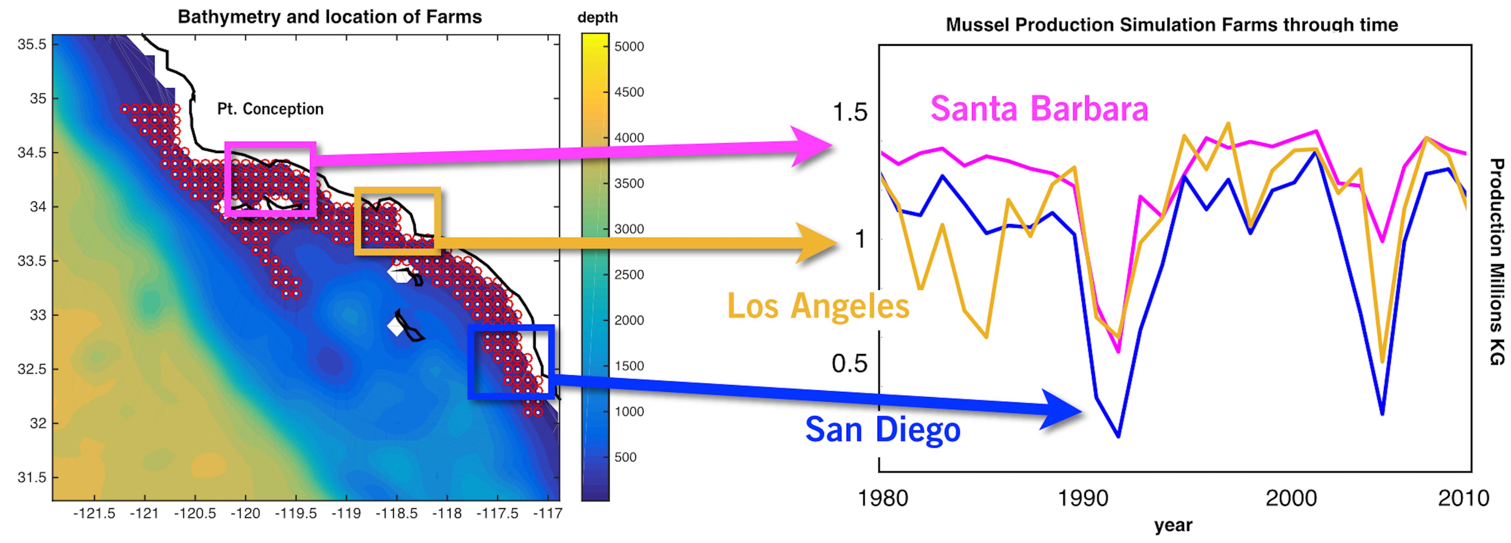
Figure 1. (Left) Coastal region of the Southern California Bight where environmental forcing was considered. The region was subdivided in 223 sites or locations (red circles). (Right) Production time series of 3 representative sites of the three main regions in the SCB, for the 1981–2008 period, as an example of variability in production year by year. Each production is calculated on an annual time step and is considering the time of harvest.

The reanalysis forcing data extracted from the UCSC Ocean Modeling and Data Assimilations website¹ was subdivided into 223 ‘sites’ along the coastal boundaries of the SCB. Each site represents a geographical location where a mussel farm is located (Figure 1).

The Mussel Production Model

In order to incorporate the effects of climate variability into mussel production, we simulated the growth of Mediterranean mussels Mytilus galloprovincialis with a Dynamic Energy Budget (DEB) model approach, adapted to aquaculture conditions. First developed by (Kooijman, 1986, 2010), the DEB theory is useful to understand functional relationships of the organisms with the environment. The central paradigm of the DEB theory is the k-rule, which describes the fractions of energy that are allocated between somatic maintenance or reproduction (Sarà et al., 2012), incorporating the uptake and use of substrates (e.g., food, nutrients, and light) by the organisms and the use of these resources for maintenance, growth, maturation and propagation by different life stages. The DEB model takes the individual as its central form of organization, but it has been applied to other organizational levels such as populations and ecological relationships (Kooijman, 2010). DEB models are also used for aquaculture and shellfish research to analyze growth and survival of bivalves in relation with environmental variables such as temperature, variable food and salinity (Pouvreau et al., 2006; Sarà et al., 2012; Maar et al., 2015). Particularly for mussels, empirical data has helped on calibrating DEB-type models, and to validate the application of this modeling approach to simulate mussel growth under variable conditions and across locations (Van Haren and Kooijman, 1993; Rosland et al., 2009; Thomas et al., 2011).

According to DEB theory, temperature ‘activates’ the basal activities of the organisms on a molecular level and directly regulates growth rates. The model is set to apply the principles of the k-rule when the mussel reaches a size of maturity and from then it starts to apportion energy toward gonads in addition to body biomass. If food supply and temperature levels are not adequate, mussels will starve.

TABLE 1

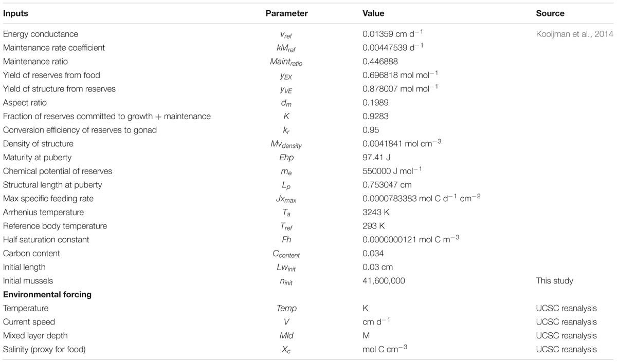
Table 1. Mussel model growth model parameters and environmental forcing variables.

The DEB model used in this project is based on the work of Muller and Nisbet (2000) which was adapted by Lester et al. (2018) to simulate mussel growth in response to four relevant environmental drivers: temperature (°C), current velocity (cm s⁻¹), mixed layer depth (m), and particulate organic carbon (POC mg cm⁻³). Biological parameters used in the model are shown in Table 1, and most of them gathered from the Add-my-Pet website² (Kooijman et al., 2014). In our analysis, the UCSC reanalysis that is used to reconstruct the historical evolution of the DEB model drivers did not contain POC. In order to estimate the time dependent changes in POC fluxes we used salinity anomalies at 50 m depth. The use of this proxy is motivated by previous studies showing a tight correlation between variations in the halocline and nutricline along the CCS (Di Lorenzo et al., 2005, Di Lorenzo et al., 2008). The salinity proxy was calibrated using an existing set of POC data for the period 2000–2001 that was used originally to develop the mussel model (Lester et al., 2018). Given that we are interested in the relative change from 1 year to the other, the calibration procedure involves adjusting the 2000–2001 mean of the salinity proxy with that from the POC dataset and re-scaling the standard deviation to match that of the POC for the same period. The resulting scaling factors are then applied to all other years.

The biological model was evaluated in order to obtain its sensitivity to environmental variables. The analysis showed that temperature and POC were the most significative forcing, explaining 51 and 42% of the productivity annual variance, while current speed and mixed layer depth only accounted for 4 and 3%, respectively. The analysis was done by running the model with small perturbations in each variable on a sequence to obtain variations of production, then fitting to least squares method to obtain the percentage of importance of each factor or variable.

In our adapted version of the DEB mussel model we simulated the change in biomass of an initial number of mussels (41,600,000) over a period of 365 days, which were seeded every year on October 1st and harvested once they reach the commercial size of 23 g. The time of harvest is an important metric for productivity used in our analysis and is calculated every year along the 28-year period. It is expected that mussels in productive sites will reach the commercial size sooner in a cultivation year, resulting in a time factor of 1 plus the fraction of the remaining year. For example, if mussels were seeded in October of 2000 and grew up to 23 g in April 2001, the site will have a factor of 1.5 because it took only 6 months for this site to reach a commercial size. The final individual weight was then multiplied by the harvest factor and the total number of individuals to calculate the final mussel production weight of the farm. This resulted variable (mussel production) was used to develop the subsequent analysis.

The model not only took into account the growth of the mussels but mortality due to starvation as well. As part of the model, death due to starvation occurs when somatic maintenance requirements cannot be met. Detrimental temperatures for mussels of 24°C (Anestis et al., 2007) are reached only in a minimum time and space for the period and region used in this study, so we expect that mortality due to temperature is not a major factor (see Appendix). Natural mortality is also not considered given the period of cultivation is just the grow out phase of the mussels. Mortality caused by predators was also set to zero.

Each of the 223 sites contained a hypothetical farm within the dimensions of 4 km². Infrastructure and production capacities can vary from farm to farm, for example, mussel farms at the Prince Edward Island Region produced ∼414 tons per km² (Department of Fisheries and Oceans, 2006); farmers in the Santa Barbara coast produce around 445 tons per km² (California Fish and Game Commission, 2018) and finally mussel farmers in Ensenada, Mexico produce 60 tons per km² (Diaz, 2018). In our case, the production capacity of each site is set for about ∼251 tons per km^2.; this means that each site would produce 1,005 tons per farm, ranging in production from 274.67 tons up to 1354.67 tons from the less to the most productive farms, after considering the additional time factor described above. Our farm arrangement was based on Lester et al. (2018) but adapted to our farm dimensions and production capacity: 32 longlines, each longline with 3,962 m of fuzzy rope, and a density of 328 mussels per m of fuzzy rope.

Historical Reconstruction of Productivity 1981–2008

Mussels were seeded each year in October and harvested when reaching commercial size at 23 g every year, over a period of 28 years from 1981 to 2008. The choice of the 1981–2008 period is motivated by the availability of a high-resolution historical reanalysis of the California Current System conducted by UCSC. This reanalysis assimilates the long-term hydrography from the CalCOFI dataset and all available satellite information with a state-of-the-art regional ocean modeling systems to generate the best available estimate of ocean conditions over this period. This simulation was computed for the 223 locations distributed over the SCB. The historical environmental data was coupled with the mussel production model to perform a hindcast of mussel production. The mussel model was run every year using environmental data for the four forcing variables that the model feeds on. With this hindcast method, time series of mussel production were obtained for the 223 sites (Figure 1). The resulting time series were used to estimate the spatial statistics and covariance analysis in order to identify profitable regions based on mean productivity and variance.

It is important to mention that spatial constraints used for the zonification of aquaculture (marine protected areas, other uses of the space) were not considered. The purpose of this study is to understand how sites gain or lose aquaculture productivity in response to environmental variability. The resulting information can be further explored for identifying ideal regions for aquaculture productivity and farms profitability.

Variability Analysis

Mean and STD

The spatial statistics over the 28 years of the mussel production hindcast were performed in order to visualize productivity and stability of production for the 223 sites (Figure 2). The mean productivity map (Figure 2A) shows high values along the coast with higher concentration south of Pt. Conception. On the other hand, the map of variance in productivity shows low values south of Pt. Conception and along the coast (Figure 2B). Taking the ratio of the mussel biomass production standard deviations over the mean (coefficient of variation) allows us to identify regions where production is stable (low values in Figure 2C) — that is the mean production is large compared to the year to year variation. This led to the recognition of three regions with clusters of sites in the North, Central and South where mussel farms are likely to be the most stable in terms of production and profit (Figure 2C). Aquaculture clusters reflect the geographical regions previously defined for the SCB as Southern Californian, and Ensenadian, having the central region of Santa Monica bay as a transition area (Blanchette et al., 2008).

FIGURE 2

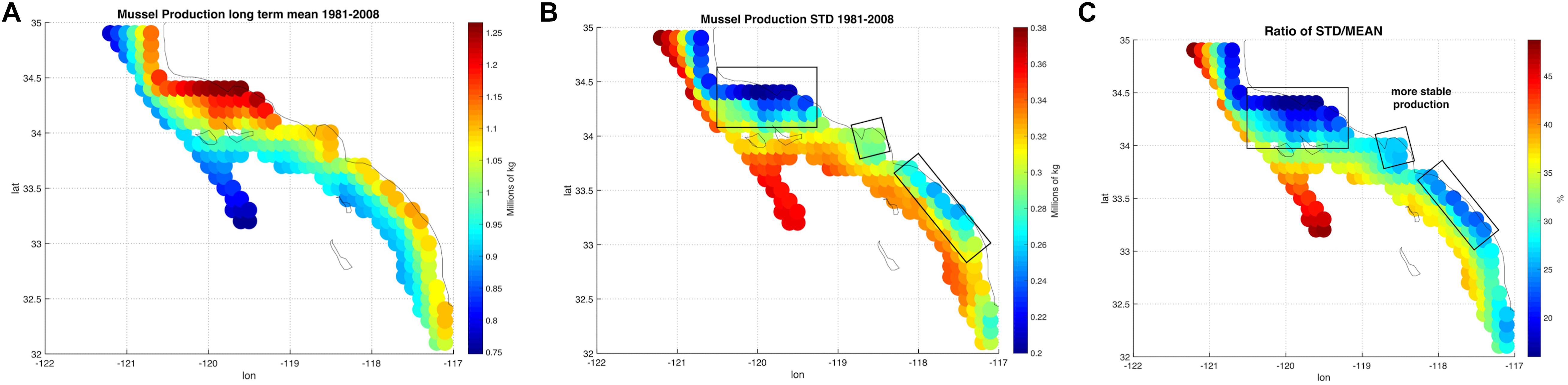
Figure 2. (A) Long-term mean of production from the mussel model along in the Southern California Bight (SCB) at the 223 sites. (B) Standard deviation of mussel production. (C) Ratio between standard deviation and long-term mean of production expressed in percentage.

EOFs and Principal Component Analysis

To characterize the variability and the level of coherence across the 223 sites, we performed Empirical Orthogonal Functions (EOF) and Principal Component Analysis (PCA) to decompose the variance map of mussel production (e.g., Figure 2B). The PCA allows to extract and quantify the coherent dominant variability across the sites (e.g., mussel farms) and understand the extent to which this variability is linked to dominant climate modes in this region. After assembling a matrix of the yearly production anomaly estimate at the end of the growing season (e.g., 1 year after the seeding of the farm in October) at each site, we computed the covariance matrix of the anomalies and decomposed it in eigenvalues and eigenvectors. The eigenvectors associated with the largest eigenvalues are referred to as EOF and correspond to the dominant spatial patterns of variability (Lorenz, 1956; Di Lorenzo et al., 2008). In the case of the mussel production, the first EOF (Figure 3A) explains 83% of the total variance and exhibits the same spatial structure as the total variance map (Figure 2B), implying that this pattern of variability is coherent across all sites. The temporal variability of the first EOF was extracted by projecting the EOF1 onto the matrix of yearly production anomaly estimates and is referred to as the first Principal Component (PC1) (Figure 3B). The time series of PC1 exhibits strong low-frequency fluctuations that are not connected to interannual events such as El Niño (e.g., there is no evidence for strong fluctuations associated with the 1982 and 1997 events). This suggest that other climate dynamics of the Pacific exert a more dominant control on mussel productions.

FIGURE 3

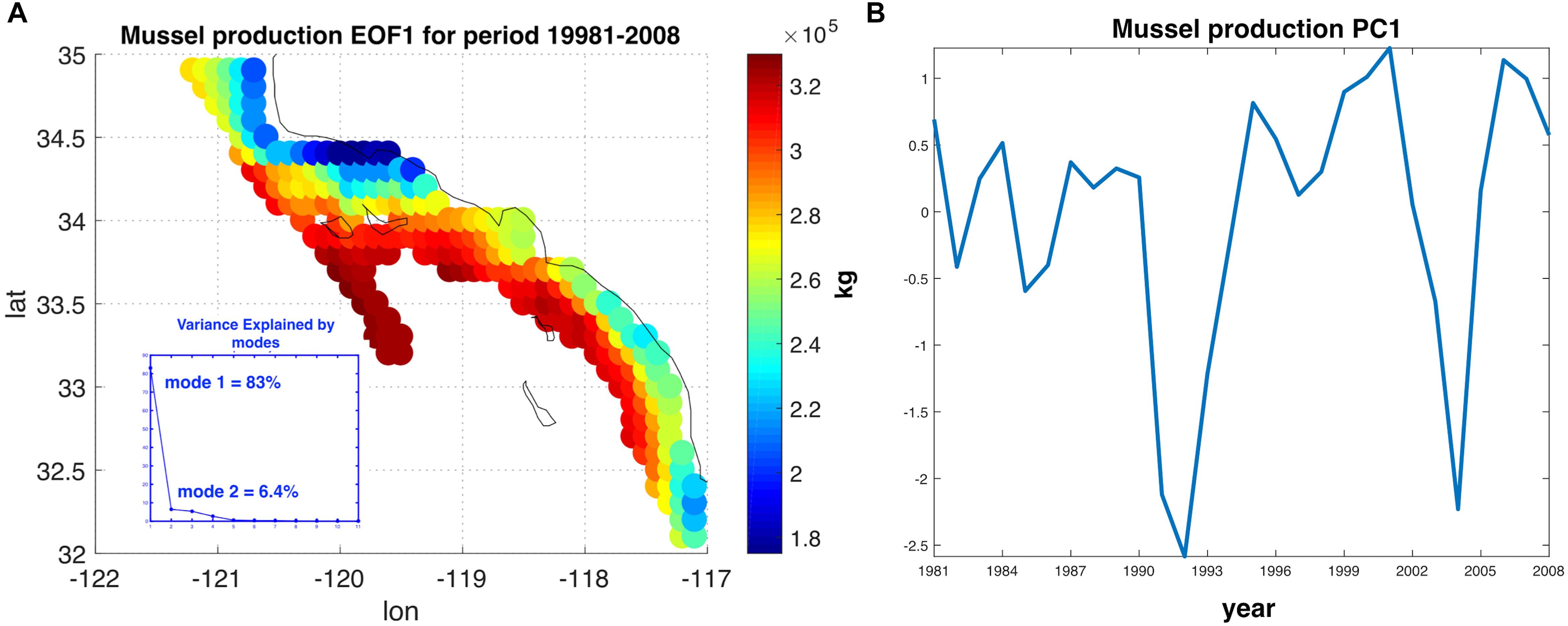
Figure 3. (A) Dominant Empirical Orthogonal Function (EOF) of the annual anomalies in mussel production. The EOF1 explains 83.08% of the interannual variability. (B) The time series associated with interannual fluctuations in EOF1, also referred to as the first Principal Component (PC1). PC1 is evaluated 20 months after the date of farm initiation due to the lag of harvest with respect on the environmental data.

Links to Pacific Climate Variability

The first mode of spatial variation (EOF1) and its temporal variation (PC1) was further explored to analyze what features of the climate are relevant for aquaculture production. The first principal component (PC1) shows synchrony (Figure 4A) and high correlation (r ≈ 0.67, p-value < 0.001) with the North Pacific Gyre Oscillation Index (Di Lorenzo et al., 2008). The relationship between modeled production and the NPGO Index is also demonstrated by the correlation of the PC1 with global sea surface temperature anomalies (SSTa from the NOAA ERSSTa v3) (Figure 4B), which exhibits the typical NPGO SSTa pattern. Mussel production variability in the SCB correlates not only locally with SSTa but with the rest of the Pacific Basic domain, demonstrating that such variability does not respond to regional scale variability but to global decadal trends associated with Pacific climate modes such as the NPGO.

FIGURE 4

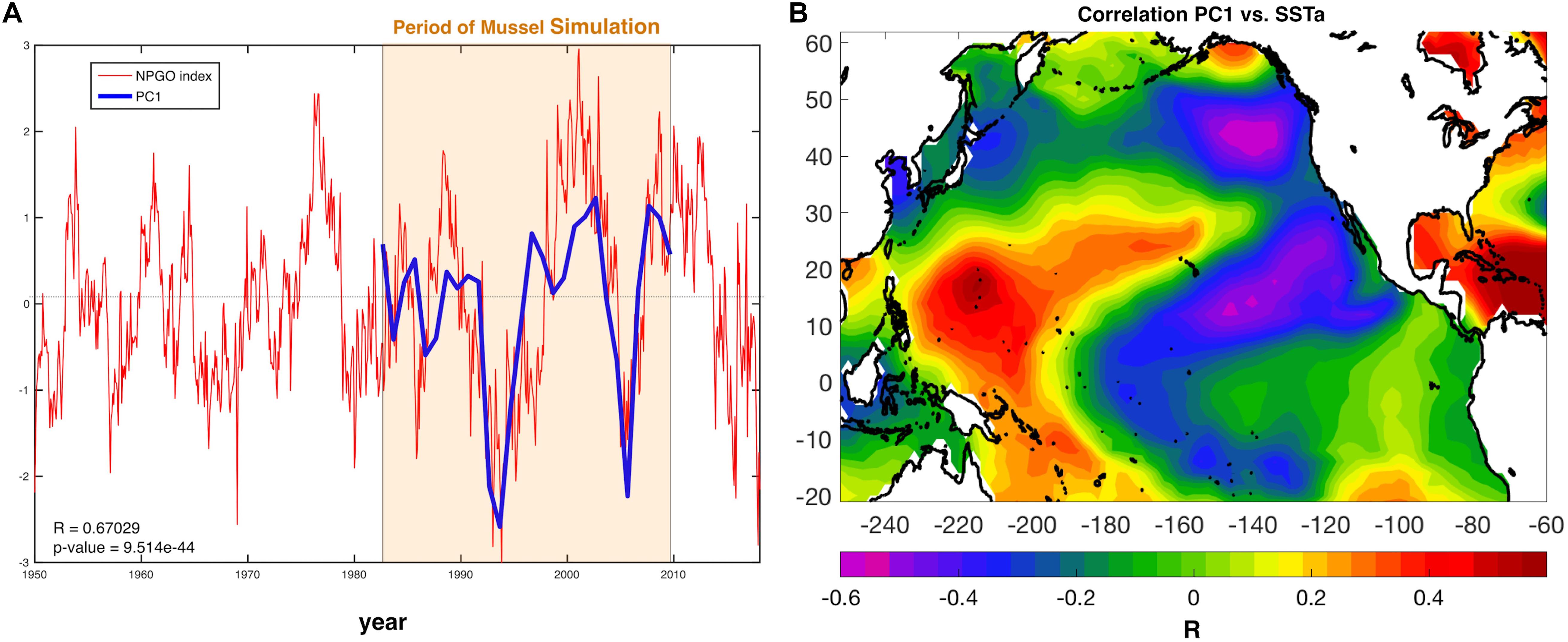
Figure 4. (A) NPGO index (red) for the entire available record and PC1 of mussel production (blue). (B) Correlation between PC1 and Pacific sea surface temperature anomalies (SSTa) reveals a large-scale climate pattern resembling the North Pacific Gyre Oscillation (NPGO).

Net Present Value and Optimal Site Selection

To analyze the effects of environmental variability over the economic value of the aquaculture sites, an economic model component is added based on the final mussel production at the end the year. The economic indicator used in this work is the Net Present Value (NPV), commonly used in economics and finance to analyze the feasibility of productive projects, including aquaculture (Whitmarsh et al., 2006; Liu and Sumaila, 2007). NPV also provides important information on the time of investment recovery and the value of the investment in present time.

The calculation of NPV (Eq. 1) utilizes information on investments and costs of running a farm minus the cash flow derived from profits of the farm. Profits are based on the revenues of selling mussels at gate price to distributers year by year. Real farms often increase their production gradually up to their maximum capacity. However, we assumed that farms would work at full capacity from the beginning (Lester et al., 2018). The discount rate selected was 8.07% which is the average for the aquaculture industry in developed countries for 1991–2015 (Ruiz Campo and Zuniga-Jara, 2018).

$$\mathit{Net\; Present\; Value}={\displaystyle \sum _{t=10}^{t=10}\frac{C_A}{{(1-\mathrm{\delta })}^t}-C_{\mathit{Init}}}\left(1\right)$$

C_Init, initial investment.

C_A, annual profits.

t, time period.

δ, discount rate.

All information on costs of running a farm were taken from Lester et al. (2018) and adapted to the characteristics of our farm model (Supplementary Table S1).

NPV: Constant vs. Variable

To show the importance of climate variability over profitability we compare a constant NPV against a variable NPV approach. Constant NPV was calculated with a constant production, using the mean production of the 28 years for each farm site simulating lack of variability in order to simulate zonification exercises where environmental conditions are assumed constant. Variable NPV was computed using the yearly production across 10 years horizons (see example in Figure 5). To do this, we selected periods of 10 years starting from 1981 until 2008; the next period would start in year 1982 and end in 1992 and so on, giving in total 18 NPV periods for each of the 223 sites. In Figure 5, we show two examples of starting the farm in different years (e.g., 1991 vs. 1993/1994) for two sites located in the Northern region and SCB. Clearly, depending on the decadal trend in a specific site, certain farms do not recover costs over the 10-year horizon (e.g., Figure 5A, red timeseries).

FIGURE 5

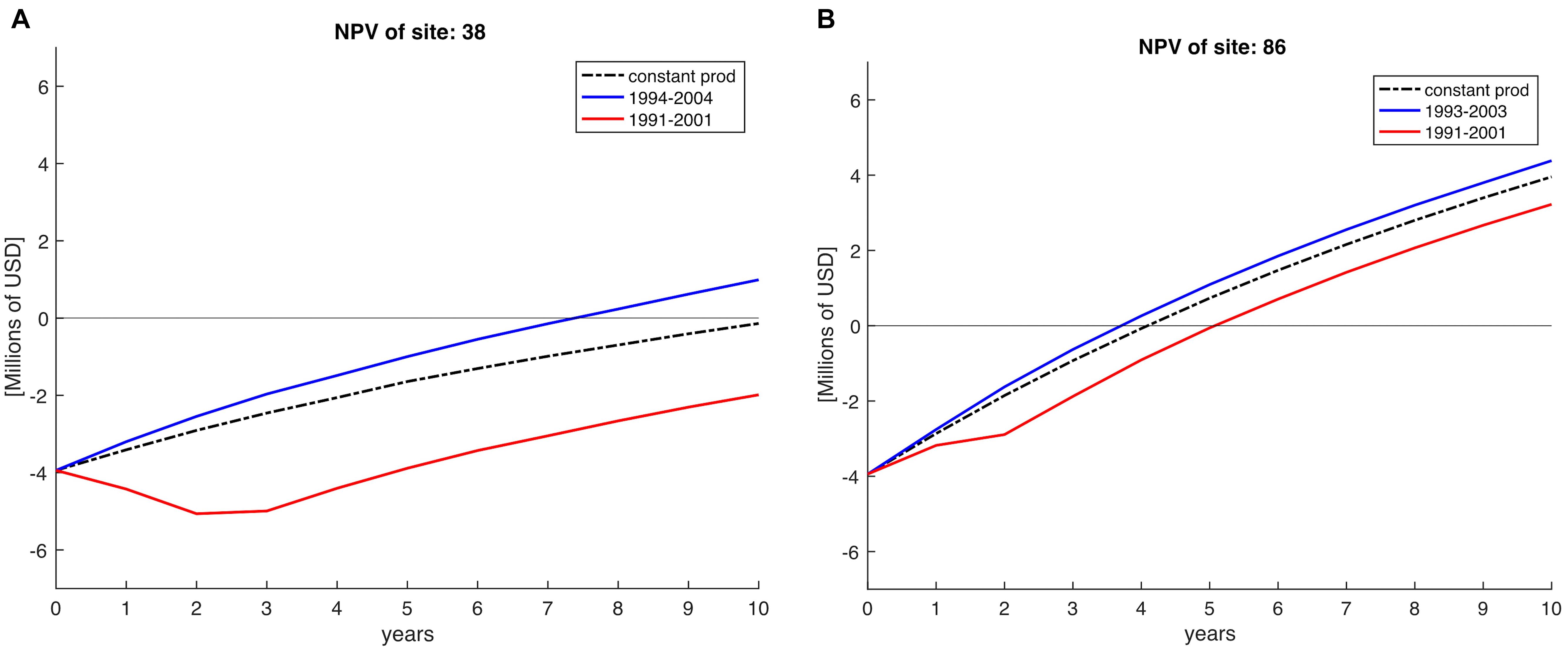
Figure 5. Net Present Value (NPV) calculations on a 10-year horizon, indicating Net Present Value for sites 38 (A) and 86 (B), both located in the Northern region of the SCB. NPV profile if calculated constant (averaged) across the 28 years of simulation is represented by the dashed black line. The red line indicates the NPV profile obtained for period 1991–2001 indicating less profits than a posterior NPV profile (blue line) calculated for periods after. Horizontal line indicates the time when the investments are recovered at the time at intersection with NPV lines.

The Ranking Procedure

A practical approach to better understand the effects of variability over site selection is a ranking system to organize all sites from best to worst based on the performance of the sites year by year. We developed two separate rankings, one for mussel productivity only and the other for NPV. Ranking both separately allows us to identify productive sites vs. sites with economic constraints, which are reflected on their NPV such as distance from port and effects of variability. The ranking procedure complements calculations of the mean and standard deviations. While spatial statistics provide useful information on productivity and stability, the ranking incorporates the variability behavior into NPV calculations and informs investors and managers with a list of best sites for mussel aquaculture, making the selection more straightforward (see Supplementary Table S2 and Supplementary Figure S1 for geographical reference).

The first rank (productivity ranking) was developed by positioning the sites from best to worst based on final weight of mussels every year. For example, the site with best tonnage and time of harvest performance will be number one at that specific year and the process continues for all the years of the environmental data available (28 years/ranking total). It is expected that sites with less variability will stay on similar positions in the ranking year by year, while sites with more variability will flip positions more drastically. A final rank is calculated to obtain the best site, based on the prior 28 years’ performance.

The second rank is calculated with the NPVs calculated for the 10 year periods. Therefore, 18 annual ranks are calculated for this particular ranking. Similar to the productivity rank, a final rank that summarizes the results of all 18 NPV periods is calculated. The top values in these rankings indicate the best sites to place farms from an economic perspective.

Results

Production of mussels varies year by year across the 28-year modeled period Figure 1. Using spatial statistics of production (Figure 2) we find that the region around Pt. Conception shows the highest yield and less overall year to year variations implying stable production rates though time. Productivity in the southern region tends to be less compared to the north and similar to the center region. Lower productivity in the southern SCB is likely linked to the seasonal presence of the warm countercurrents coming from the South (DiGiacomo and Holt, 2001) and a stronger effect of variability over temperatures in these areas (Kim and Cornuelle, 2015). However, the southern region tends to be more stable than the center. Some sites in the southern portions of the SCB show high mean production and low standard deviations exhibiting more spatial heterogeneity compared to the north. Sites where the mean production is highest are also the sites where the time of harvest is shorter – that is mussels reach the harvest size sooner (Figure 6).

FIGURE 6

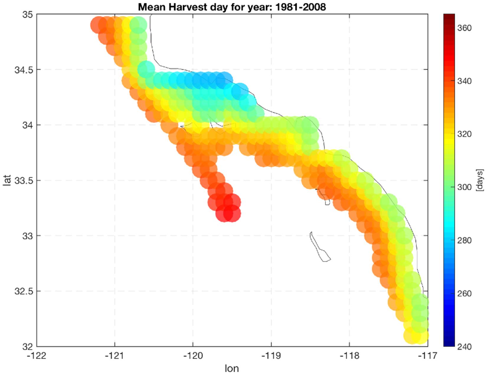
Figure 6. Mean harvest time length. Color indicate the number of days required to grow mussels up to the commercial size (23 g).

Along the coast, overall production values are higher compared to offshore locations. Sites closer to the coast show a low std/mean ratio compared offshore sites, which are characterized by high values of the std/mean ratio (>30%) implying less sustained production and more interannual uncertainties. Offshore waters tend to be more oligotrophic than coastal waters in the SCB (Eppley, 1992; Kim et al., 2009) which explains this productivity gradient from the shore.

Despite the yearly variability in production Figure 1, there is evidence of significant low-frequency variability that gives rise to decadal trends in the time series of production. This behavior was analyzed and linked to climate regimes of the SCB. The EOF decomposition of the variance of mussel production (Figure 3) shows that the first mode (EOF1) recovers the main features of the standard deviation pattern (a), which account for the largest fraction of variance (∼83%). The temporal variability of this pattern shown by PC1 (b) confirms a very strong low-frequency variability shared across all sites. Given that the farms have no memory from one year to the next (i.e., farms are re-seeded every year), the low-frequency changes must be associated with cumulative integration effects associated with the environmental drivers (e.g., SSTa, mixed layer depth, current speed, and food supply; e.g., Di Lorenzo and Ohman, 2013). Interestingly, there was no clear signature of interannual variations associated with the El Niño Southern Oscillation (ENSO) and most of the variance was on decadal timescales. Further analyses of the PC1 revealed that the low-frequency variance is linked with the regional expressions of large-scale climate variability in the Pacific Basin (Figure 4B), specifically the NPGO mode.

In terms of profitability of the sites, the North region shows high NPV and stability. Recovery times are shorter than the other two regions (around 4 years). These two aspects give the northern region an advantage over the other two regions. As mentioned before, productivity in the south is less than the center but stability is better. Not surprisingly, the NPV in the center region is less stable than the North and the South and recovery times can also take longer (from 4 up to 8.5 years). The lack of profitability in some sites can be attributed to economic factors (long distance from ports) or being located in an unsuitable environmental conditions for mussel growth.

The calculation of all 18 NPV periods also displayed spatial and temporal heterogeneity. All regions’ NPV curves vary depending on the time periods where projects initiate. This means that there are good productions during specific time periods, so a temporal component related to productivity and profits is also identified. Given the principal component analysis pointed at the NPGO as the main driver for mussel productivity, we matched the NPV profiles with the numerical index to illustrate possible effects of decadal variability over profitability of the farms. As representative examples, during 1988–1998 the NPGO index is moving toward a negative phase and during the period 1990–2000 the index stays on negative (Figure 7A). In contrast, period 1994–2004 shows upward direction indicating transition toward a positive phase, and finally period 1997–2007 is mostly positive. These four periods were linked with NPVs of representative farm sites of the identified northern, center and southern regions Figures 7B–D.

FIGURE 7

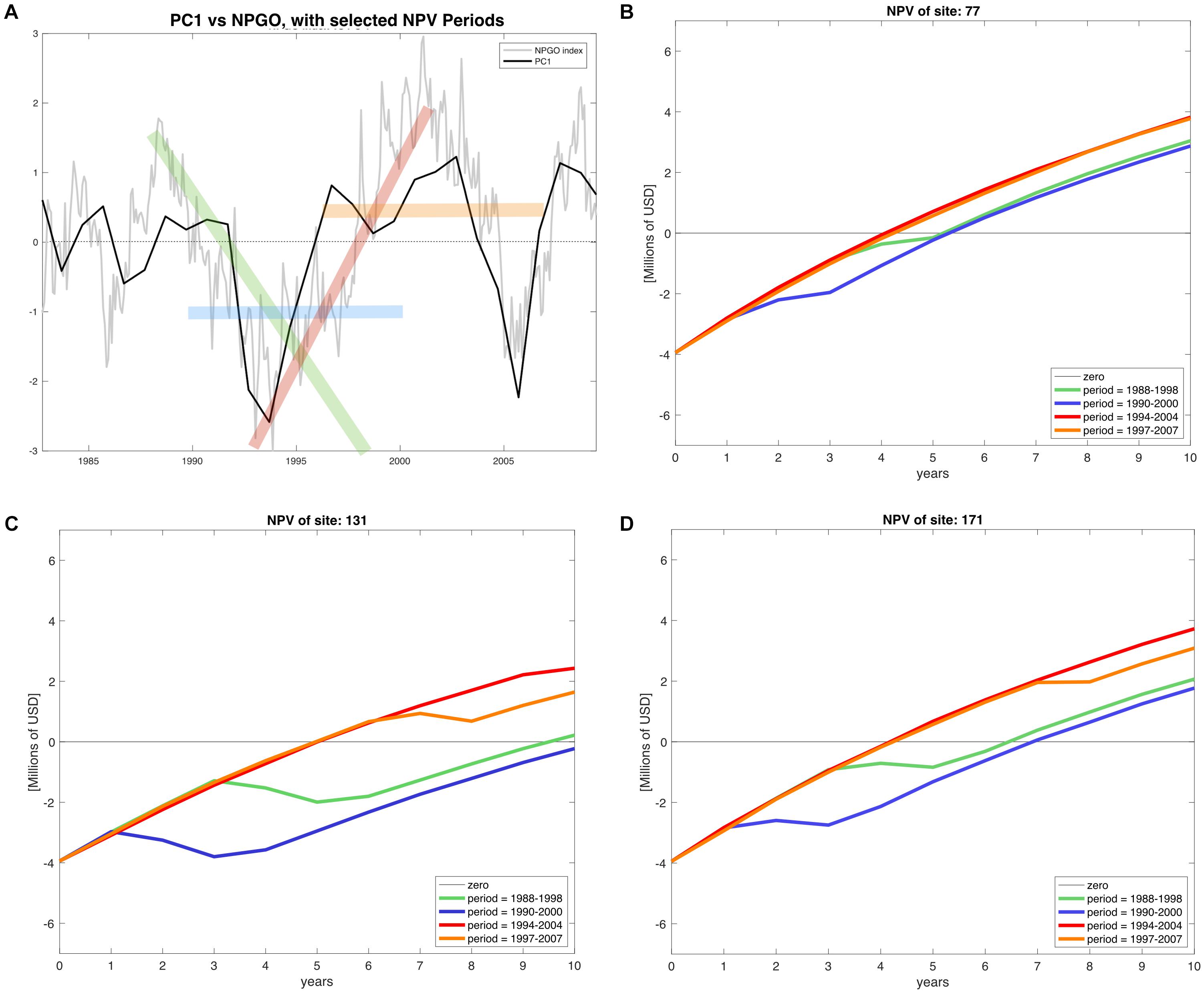
Figure 7. (A) NPGO index (gray) for the period of available environmental data (1981–2008) and PC1 of modeled mussel production (black). The time periods highlighted in green (1988–1998), blue (1990–2000), red (1994–2004), and orange (1997–2007) indicate different phases of the NPGO. (B–D) NPV profiles of the corresponding stages of NPGO for representative sites of the north, center and south of the SCB.

The profitability at all sites depends on the phase of the NPGO. For example, on Table 2 the periods 1988–1998 and 1990–2000, both considered to be negative, result in a drop in NPVs, while in the following two periods the profitability is considerably higher, and all sites follow this behavior. The critical period in terms of profitability is 1990–2000, where most sites dropped profitability compared to other periods. Choosing to start a project in this period results in economic loss for sites with less productivity and highly sensitive to variability. Period 1994–2004 displays the best NPVs for all the sites, which indicates good timing to initiate an aquaculture project of this nature.

Best ranked sites are highly productive (>1,000 tons annually, based on its global long term mean) and the variation low compared to their mean production values (<0.26 std/mean ratio). If ranked by production, the northern region concentrates most of the top sites (Figure 8A). Not surprisingly, site 97 located in the northern region was found to be rated the top site of the productivity ranking (Figure 8A). However, the NPV ranking (Figure 8B) was more heterogeneous.

FIGURE 8

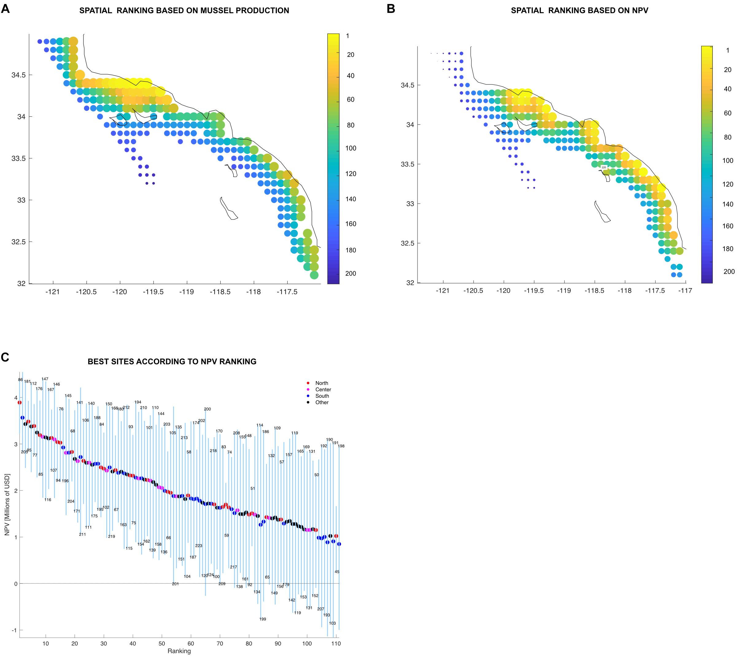
Figure 8. (A,B) Individual ranking displayed spatially showing top sites in yellow down to bad sites in dark blue. Color bar and the size of the marker indicates the site rank. (C) Farm sites above the mean organized from best to worst displaying the minimum and maximum (blue vertical lines) and average (colored dots) values in million USD (Y-axis). The X-axis shows the ranking order, where sites organized from best to worst. Sites are represented by each of the blue vertical lines and the color on the average dot represent the region where the site is located. The numbers above and below the vertical lines are the site identification numbers. Legend shows the number of sites in each region and the proportion of total sites.

Discussion

Variability is a big challenge for aquaculture developed in the marine environment. Efforts to understand the effects of variability include seasonal forecasts, which provide farmers with reliable climate information to plan along with the environmental forcing from week to months ahead (Spillman and Hobday, 2014; Hobday et al., 2016). Climate change is considered a problem of longer time scale, expected to alter variables important for bivalve productivity. GIS suitability methods (Handisyde et al., 2006; Saitoh et al., 2011; Liu et al., 2013; Aura et al., 2017) and end-to-end models address productivity under ocean acidification and carrying capacity (Bell et al., 2013; Guyondet et al., 2015) to identify winner and loser species (Filgueira et al., 2016; Froehlich et al., 2018), and provide a very complete understanding on how the environment influences mussel performance in a farm (Matzelle et al., 2015). In general, this particular body of work is based on a sensitivity-type approach, where key variables for bivalve production are changed based on the most feasible scenarios projected for climate change in the future.

TABLE 2

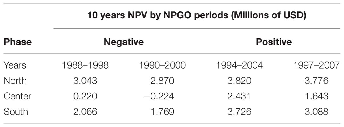
Table 2. Resulting NPV for four different periods of representative sites matching with negative (1988–1998, 1990–2000) and positive (1994–2004, 1997–2007) phases of the NPGO.

Our work presents two methods that help incorporate climate variability into zoning plans for aquaculture and site selection. First, we propose EOFs and PC analysis to identify what decadal trends are the most important depending on the region and species that are planned to be cultivated, and the ranking method can inform decisions for selection and valuation of sites which is important for managers, investors and farmers. A key difference with previous work is that we approached aquaculture production as time dependent based on the historical evolution of environmental forcing. In this context, modeled mussel production time series in the SCB showed dependence on decadal fluctuation, which is consistent with positive and negative phases of the NPGO. The calculation of the NPV is inherently a time dependence problem because is calculated according to continuous years of costs and profits.

Time dependence is also reflected on the ranking system developed in this work. The results from a single year of mussel aquaculture production in the SCB could lead stakeholders to assume that all sites found in the north are the most profitable. However, adding variability led to interesting results. An analysis of the production ranking shows that certainly, the majority of the good sites are found in the north, but it also shows some good sites in the south (Figure 8A). Local oceanographic conditions might play an important role on this. For example, site 205 which is located in the region south (North San Diego) has the 27th place on the production rank (Supplementary Table S2). North San Diego has been found to have an important nutrient flux from upwelling (Howard et al., 2014). A sudden change on the spatial trend occurs in the NPV rank (Figures 8B,C). Productive and profitable farm sites can be found across all the SCB. Sites found in the central and southern regions, as well as outside of the identified clusters in the statistical analysis were above the ranking’s mean. The reason for this behavior is that NPV rank summarizes the interplay between productivity, variability and the economics of the sites (distance from ports, wave height, etc). The proposed ranking system thus provides additional criteria for spatial planning and allocation of aquaculture areas and increases the resolution for site selection.

It is clear that there are sites that are less productive which results in lower income (NPV), but since the production of those sites are more stable, their incomes are quite constant over all periods. Such sites have stability that allows decisions on expansion with low risk (e.g., site 180, located at region south). On the other hand, there are sites that are highly productive but their fluctuations rate them as optimal in some periods and causing losses in other periods (e.g., site 124, at the Central region of the SCB) (Supplementary Table S2). This behavior may encourage adaptive spatial management for marine aquaculture: sites could produce other species during decades when mussels are not profitable.

There is little empirical work that directly links productivity of farms with climate trends has been developed in comparison to other food production sectors such as fisheries. ENSO has been found to have effects over productivity of cultured green mussels in New Zealand due to indirect inputs on nutrients (Zeldis et al., 2008) and over calcification and growth in scallops cultivated in an upwelling region in Chile (Lagos et al., 2016). Despite the big influence of ENSO over regional productivity, we did not find significant correlation with ENSO. The productivity signal of ENSO appears to be more relevant during certain years depending on its strength (Kahru and Mitchell, 2000; Bograd and Lynn, 2001; Kim et al., 2009). ENSO influences precipitation in the SCB (Schonher and Nicholson, 1989; Cayan et al., 1999) and such indirect effects over mussel productivity could be explored using this historical approach in combination with end-to-end models mentioned above adapted to this goal. Adequate environmental data resolution and quality are relevant to approach the effects of climate and aquaculture performance through modeling (Montalto et al., 2014).

Availability of mussel larvae is very important for farmers who in most cases capture mussel spat from the wild. Reduced mussel larvae abundance followed a seawater chlorophyll-a concentration weakening in 2009–2010 that coincides with positive phases of MEI and PDO in Northern Patagonia, Chile (Lara et al., 2016). For study sites in Oregon, the role of the NPGO is relevant on recruitment and food availability (Menge et al., 2009) and filtration rates of later stages of mussels (Menge et al., 2011) which potentially reinforces the relationship between the NPGO and aquaculture success. The SCB region seems to have more heterogeneous patterns in recruitment and growth in comparison with Northern California (Smith et al., 2009), so further empirical work is required to confirm the influence of the NPGO over these variables for recruitment and growth of mussels in the SCB. This opens a window to link ecological research and aquaculture productivity, in collaboration with the aquaculture industry in the SCB. Analysis of mussel larvae along with grow out experiments are two possible paths to corroborate the findings of our modeling work.

The Importance of Natural Decadal Variability

The initial focus of this study was to evaluate the role of interannual variability (e.g., ENSO) because the initial annual runs revealed a year by year variation on the productivity of mussel farms in the SCB. However, our results revealed that the decadal-scale variability associated with large-scale Pacific climate may be more important in planning frameworks for mussel aquaculture. The EOFs analysis demonstrated that mussel productivity in the SCB is highly coherent in space and correlated to the decadal variability of the NPGO compared to little influence of interannual-like phenomena like ENSO.

The emergence of decadal-scale fluctuations in the mussel production as opposed to interannual events is ascribed to the fact that farms are sensitive to multiple drivers. The integration of these multiple forcing tends to extract and amplify the lowest frequency variability that is common to the different drivers (Di Lorenzo and Ohman, 2013). It is likely that productivity of aquaculture farms of other species that rely on multiple environmental drivers like food and temperature (e.g., bivalves and algae) will also have similar decadal fluctuations. For example, decadal oscillations of natural giant kelp forests have been linked to the NPGO in California (Bell et al., 2015; Blanchette et al., 2008). Future kelp aquaculture in the SCB will likely be affected in a similar fashion. In contrast, assuming that oxygen is not limiting, farmed fish which are highly sensitive to temperature may exhibit stronger interannual variability associated with the ENSO extremes.

Decadal forcing is known to impact ecosystems in the Pacific Basin (King et al., 2011) and the California Current upwelling system (Chhak and Di Lorenzo, 2007; Di Lorenzo et al., 2008; Bell et al., 2015, 2018). The NPGO index is earning increasing relevance in explaining productivity switching regimes with important consequences on marine ecosystems along the California Current (Di Lorenzo et al., 2008), including the Southern California Bight (Nezlin Nikolay et al., 2017).

Decadal-scale variability has also been observed in natural populations of the Greenland smooth cockle Serripes groenlandicus in the Barents Sea, where growth mechanisms were correlated to increased riverine discharge influenced by a negative phase of the North Atlantic Oscillation Index (NAO) (Carroll et al., 2009).

There is a strong relationship between the NPV and decadal trends. NPV periods that coincide with negative phases of the NPGO display a generalized reduction in profitability. However, there is spatial heterogeneity on how the farm sites respond to negative phases of the NPGO. On the other hand, the positive periods also move profitability up at most of the sites. This can be critical especially when starting a new aquaculture venture when big investments are at risk.

The results of our bioeconomic analysis highlights the possibility of predicting production based on the decadal climate state. From a management perspective, dependence of mussel aquaculture on decadal fluctuations is a remarkable statement: there are decades of ‘good years’ and decades of ‘bad years’ for mussel aquaculture. Although is still unclear the extent to which these climate decades can be predicted (Meehl et al., 2010, 2016; Liu and Di Lorenzo, 2018), this information would allow managers and investors to plan accordingly the best times to invest in such venture.

Conclusion

The effect of the variable behavior of production of mussels over site selection of aquaculture was an initial motivation of this work. Our climate sensitive analysis of productivity showed that the spatial heterogeneity of the SCB as well as its climate regimes resulted in a variable panorama in production and profitability that raises questions on the use of constant environmental conditions (e.g., temperature and nutrient fluxes) in the spatial planning of aquaculture farms such as mussels.

Our results indicate that climate variability is a key component of the site selection process for marine aquaculture. Finding a good site location is important, however, selecting the right time to start a mussel farm is also key to success. We highlight the importance of taking into account decadal trends in addition to the short term climate.

The strong relationship between decadal variability and mussel productivity in the SCB resulted in different investment recovery scenarios. This decadal trend causes alternation in the profitability between “good” and “bad”: decades of some farm sites. Understanding aquaculture planning in the context of marine climate variability is critical for the planning and zonification of marine aquaculture. In addition, this knowledge can benefit managers and investors because they will be able to know when to expand, move, hold, or change the species to be farmed in order to keep the food and investment security.

We propose that the industry and all stakeholders involved in spatial planning of marine aquaculture consider environmental variability and climate trends that might be crucial for the success of their operations.

Considerations About the Impact of Climate to Be Further Explored

Although this study only considered four environmental variables in mussel farms simulations, the framework presented here can be improved with the addition of variables important for aquaculture production. Such variables include the effects of harmful algal blooms (HABs), hypoxia and ocean acidification, particularly because of recent climate extremes that led to prolonged warm events and HABs along the California Current (Moore et al., 2008; Hallegraeff, 2010; Gruber, 2011). Although upwelling is the main source of nutrients in the SCB (Howard et al., 2014), additional sources of nutrient inputs should also be considered. For example runoff in the SCB is strongly influenced by interannual variability in precipitation (i.e., El Niño) (Nezlin and DiGiacomo, 2005).

Stronger North Pacific decadal variability in the Northeast Pacific is also predicted in future climate (Joh and Di Lorenzo, 2017; Liguori and Di Lorenzo, 2018), so the effects of changes in such mechanisms must be also be explored because they may lead to decades of enhanced profit but also decades of extreme loss.

Author Contributions

JS: scientific idea, analysis, and writing. EDL: scientific idea, climate data gathering, and analysis. TB: scientific idea, data collection, and editing. SG, RM, and HL scientific idea and editing.

Funding

JS was supported by UC MEXUS-CONACyT Doctoral Fellowship and the Latin American Fisheries Fellowship of the Walton Family Foundation.

Conflict of Interest Statement

The authors declare that the research was conducted in the absence of any commercial or financial relationships that could be construed as a potential conflict of interest.

Acknowledgments

We thank Sarah Lester, Rebecca Gentry, Casey Maue, and the NOAA Sea Grant Project No. (#NA10OAR4170060, California Sea Grant College Program Project #R/AQ-134) for providing biological data on mussels and supporting the development of the study. Modeling support was also provided through the CCE-LTER grant.

Supplementary Material

The Supplementary Material for this article can be found online at: https://www.frontiersin.org/articles/10.3389/fmars.2019.00253/full#supplementary-material

Footnotes

1. ^ http://oceanmodeling.pmc.ucsc.edu
2. ^ https://www.bio.vu.nl/thb/deb/deblab/add_my_pet/

References

Airamé, S., Dugan, J. E., Lafferty, K. D., Leslie, H., McArdle, D. A., and Warner, R. R. (2003). Applying ecological criteria to marine reserve design: a case study from the California Channel Islands. Ecol. Appl. 13(Suppl. 1), 170–184. doi: 10.1890/1051-0761(2003)013

CrossRef Full Text | Google Scholar

Anestis, A., Lazou, A., Pörtner, H. O., and Michaelidis, B. (2007). Behavioral, metabolic, and molecular stress responses of marine bivalve Mytilus galloprovincialis during long-term acclimation at increasing ambient temperature. Am. J. Physiol. Regul. Integr. Comp. Physiol. 293, R911–R921. doi: 10.1152/ajpregu.00124.2007

PubMed Abstract | CrossRef Full Text | Google Scholar

Aura, C. M., Musa, S., Osore, M. K., Kimani, E., Alati, V. M., Wambiji, N., et al. (2017). Quantification of climate change implications for water-based management: a case study of oyster suitability sites occurrence model along the Kenya coast. J. Mar. Syst. 165, 27–35. doi: 10.1016/j.jmarsys.2016.09.007

CrossRef Full Text | Google Scholar

Bell, J. D., Ganachaud, A., Gehrke, P. C., Griffiths, S. P., Hobday, A. J., Hoegh-Guldberg, O., et al. (2013). Mixed responses of tropical Pacific fisheries and aquaculture to climate change. Nat. Clim. Change 3, 591–599. doi: 10.1038/nclimate1838

CrossRef Full Text | Google Scholar

Bell, T. W., Allen, J. A., Cavanaugh, K. C., and Siegel, D. A. (2018). Three decades of variability in California’s giant kelp forests from the Landsat satellites. Remote Sens. Environ. (in press). doi: 10.1016/j.rse.2018.06.039

CrossRef Full Text | Google Scholar

Bell, T. W., Cavanaugh, K. C., Reed, D. C., and Siegel, D. A. (2015). Geographical variability in the controls of giant kelp biomass dynamics. J. Biogeogr. 42, 2010–2021. doi: 10.1111/jbi.12550

CrossRef Full Text | Google Scholar

Blanchette, C. A., Melissa Miner, C., Raimondi, P. T., Lohse, D., Heady, K. E. K., and Broitman, B. R. (2008). Biogeographical patterns of rocky intertidal communities along the Pacific coast of North America. J. Biogeogr. 35,1593–1607. doi: 10.1111/j.1365-2699.2008.01913.x

CrossRef Full Text | Google Scholar

Bograd, S. J., and Lynn, R. J. (2001). Physical-biological coupling in the California current during the 1997–99 El Niño-La Niña Cycle. Geophys. Res. Lett. 28, 275–278. doi: 10.1029/2000GL012047

CrossRef Full Text | Google Scholar

Bograd, S. J., and Lynn, R. J. (2003). Long-term variability in the southern California current system. Deep Sea Res. II Top. Stud. Oceanogr. 50, 2355–2370. doi: 10.1016/s0967-0645(03)00131-0

CrossRef Full Text | Google Scholar

Bostock, J., McAndrew, B., Richards, R., Jauncey, K., Telfer, T., Lorenzen, K., et al. (2010). Aquaculture: global status and trends. Philos. Trans. R. Soc. B Biol. Sci. 365, 2897–2912.

Google Scholar

Bray, N. A., Keyes, A., and Morawitz, W. M. L. (1999). The California current system in the Southern California bight and the Santa Barbara Channel. J. Geophys. Res. Oceans 104, 7695–7714. doi: 10.1029/1998JC900038

CrossRef Full Text | Google Scholar

Briggs, J. C., and Bowen, B. W. (2011). A realignment of marine biogeographic provinces with particular reference to fish distributions. J. Biogeogr. 39, 12–30. doi: 10.1111/j.1365-2699.2011.02613.x

CrossRef Full Text | Google Scholar

Bryniarski, A. (2015). “California aquaculture law symposium: summary report,” in Proceedings of the National Sea Grant Law Center - Resnick Program for Food Law and Policy at the UCLA School of Law, (Los Angeles).

Google Scholar

Buck, B. H., Ebeling, M. W., and Michler-Cieluch, T. (2010). Mussel cultivation as a co-use in offshore wind farms: potential and economic feasibility. Aquac. Econ. Manag. 14, 255–281. doi: 10.1080/13657305.2010.526018

CrossRef Full Text | Google Scholar

California Fish and Game Commission (2018). Initial Study and Mitigated Negative Declaration for Santa Barbara Mariculture Company Continued Shellfish Aquaculture Operations on State Water Bottom Lease Offshore Santa Barbara. California, CA: California Fish and Game Commission.

Google Scholar

CaliforniaSeaGrant (2015). How can we Grow Aquaculture in California?. Available at: https://caseagrant.ucsd.edu/news/how-can-we-grow-aquaculture-in-california (accessed October, 2017).

Google Scholar

Callaway, R., Shinn, A. P., Grenfell, S. E., Bron, J. E., Burnell, G., Cook, E. J., et al. (2012). Review of climate change impacts on marine aquaculture in the UK and Ireland. Aquat. Conserv.: Mar. Freshw. Ecosyst. 22, 389–421. doi: 10.1002/aqc.2247

PubMed Abstract | CrossRef Full Text | Google Scholar

Carr, M.-E. (2001). Estimation of potential productivity in Eastern Boundary currents using remote sensing. Deep Sea Res. II Top. Stud. Oceanogr. 49, 59–80. doi: 10.1016/S0967-0645(01)00094-7

CrossRef Full Text | Google Scholar

Carroll, M. L., Johnson, B. J., Henkes, G. A., McMahon, K. W., Voronkov, A., Ambrose, W. G., et al. (2009). Bivalves as indicators of environmental variation and potential anthropogenic impacts in the southern Barents Sea. Mar. Pollut. Bull. 59, 193–206. doi: 10.1016/j.marpolbul.2009.02.022

PubMed Abstract | CrossRef Full Text | Google Scholar

Cayan, D. R., Redmond, K. T., and Riddle, L. G. (1999). ENSO and hydrologic extremes in the Western United States. J. Clim. 12, 2881–2893. doi: 10.1175/1520-04421999012<2881:EAHEIT<2.0.CO;2

CrossRef Full Text | Google Scholar

Chhak, E. (2007). Decadal variations in the California Current upwelling cells. Geophys. Res. Lett. 34:L14604. doi: 10.1029/2007GL030203

PubMed Abstract | CrossRef Full Text | Google Scholar

Chivers, S. J., Perryman, W. L., Lynn, M. S., Gerrodette, T., Archer, F. I., Danil, K., et al. (2015). Comparison of reproductive parameters for populations of eastern North Pacific common dolphins: Delphinus capensis and D. delphis. Mar. Mamm. Sci. 32, 57–85. doi: 10.1111/mms.12244

CrossRef Full Text | Google Scholar

Cochrane, K., De Young, C., Soto, D., and Bahri, T. (2009). “Climate change implications for fisheries and aquaculture,” in FAO Fisheries and Aquaculture Technical Paper, eds B. F. Phillips and M. Pérez-Ramírez (FAO: Rome).

Google Scholar

Cohen, J. (2017). Cultivating Marine Biomass. Available at: http://www.news.ucsb.edu/2017/018267/cultivating-marine-biomass (accessed November, 2017)

Google Scholar

Daley, M. D., Jack, A. W., Reish, D. J., Gorsline, D. S., and Anderson Pages. (1993). “The Southern California bight, background and setting,” in Ecology of the Southern California Bight: a Synthesis and Interpretation, eds D. J. R. Murray, D. Dailey, and J. W. Anderson (Berkeley, CA: University of California Press), 1–18.

Google Scholar

Department of Fisheries and Oceans (2006). An Economic Analysis of the Mussel Industry in Prince Edward Island, Gulf Region. Moncton, NB: Department Fisheries and Ocens.

Google Scholar

Di Lorenzo, E. (2003). Seasonal dynamics of the surface circulation in the Southern California Current System. Deep Sea Res. II Top. Stud. Oceanogr. 50, 2371–2388. doi: 10.1016/S0967-0645(03)00125-5

CrossRef Full Text | Google Scholar

Di Lorenzo, E., Fiechter, J., Schneider, N., Bracco, A., Miller, A. J., Franks, P. J. S., et al. (2009). Nutrient and salinity decadal variations in the central and eastern North Pacific. Geophys. Res. Lett. 36:L14601. doi: 10.1029/2009GL038261

CrossRef Full Text | Google Scholar

Di Lorenzo, E., Miller, A. J., Schneider, N., and McWilliams, J. C. (2005). The warming of the california current system: dynamics and ecosystem implications. J. Phys. Oceanogr. 35, 336–362. doi: 10.1175/JPO-2690.1

CrossRef Full Text | Google Scholar

Di Lorenzo, E., and Ohman, M. D. (2013). A double-integration hypothesis to explain ocean ecosystem response to climate forcing. Proc. Natl. Acad. Sci. U.S.A. 110, 2496–2499. doi: 10.1073/pnas.1218022110

PubMed Abstract | CrossRef Full Text | Google Scholar

Di Lorenzo, E., Schneider, N., Cobb, K. M., Franks, P. J. S., Chhak, K., Miller, A. J., et al. (2008). North Pacific Gyre Oscillation links ocean climate and ecosystem change. Geophys. Res. Lett. 35:L08607. doi: 10.1029/2007GL032838

PubMed Abstract | CrossRef Full Text | Google Scholar

Diana, J. S., Egna, H. S., Chopin, T., Peterson, M. S., Cao, L., Pomeroy, R., et al. (2013). responsible aquaculture in 2050: valuing local conditions and human innovations will be key to success. BioScience 63, 255–262. doi: 10.1525/bio.2013.63.4.5

CrossRef Full Text | Google Scholar

Diaz, I. (2018). Datos Abiertos de Producción Acuícola y Pesquera, 2014. Available at: https://datos.gob.mx/busca/dataset/produccion-pesquera. (accessed September, 2017).

Google Scholar

DiGiacomo, P. M., and Holt, B. (2001). Satellite observations of small coastal ocean eddies in the Southern California Bight. J. Geophys. Res. Oceans 106, 22521–22543. doi: 10.1029/2000JC000728

CrossRef Full Text | Google Scholar

Eppley, R. W. (1992). Chlorophyll, photosynthesis and new production in the Southern California Bight. Prog. Oceanogr. 30, 117–150. doi: 10.1016/0079-6611(92)90010-W

CrossRef Full Text | Google Scholar

FAO (2016). The State of World Fisheries and Aquaculture 2016. Contributing to food security and nutrition for all. Rome: Food & Agriculture Org.

Google Scholar

Filgueira, R., Guyondet, T., Comeau, L. A., and Tremblay, R. (2016). Bivalve aquaculture-environment interactions in the context of climate change. Global Change Biol. 22, 3901–3913. doi: 10.1111/gcb.13346

PubMed Abstract | CrossRef Full Text | Google Scholar

Froehlich, H. E., Gentry, R. R., and Halpern, B. S. (2018). Global change in marine aquaculture production potential under climate change. Nat. Ecol. Evol. 2, 1745–1750. doi: 10.1038/s41559-018-0669-1

PubMed Abstract | CrossRef Full Text | Google Scholar

Froehlich, H. E., Gentry, R. R., Rust, M. B., Grimm, D., and Halpern, B. S. (2017). Public perceptions of aquaculture: evaluating spatiotemporal patterns of sentiment around the world. PLoS One 12:e0169281. doi: 10.1371/journal.pone.0169281

PubMed Abstract | CrossRef Full Text | Google Scholar

Gaylord, B., Rivest, E., Hill, T., Eric, S., Shukla, P., and Ninokawa, A. (2018). “California mussels as bio-indicators of the ecological consequences of global change: temperature, ocean acidification, and hypoxia,” in Proceedings of the 4th California’s Climate Change Assessment, (Sacramento, CA: California Natural Resources Agency).

Google Scholar

Gentry, R. R., Lester, S. E., Kappel, C. V., Stevens, J., White, C., Bell, T. W., et al. (2017b). Offshore aquaculture: spatial planning principles for sustainable development. Ecol. Evol. 7, 733–743. doi: 10.1002/ece3.2637

PubMed Abstract | CrossRef Full Text | Google Scholar

Gentry, R. R., Froehlich, H. E., Grimm, D., Kareiva, P., Parke, M., Rust, M., et al. (2017a). Mapping the global potential for marine aquaculture. Nat. Ecol. Evol. 1, 1317–1324. doi: 10.1038/s41559-017-0257-9

PubMed Abstract | CrossRef Full Text | Google Scholar

Grant, C. G., Brianna, G., Ho, D., Read, E., and Winslow, E. (2017). Planning and Incentivizing Native Olympia Oyster Restoration in Southern California. Master’s thesis, University of California, Santa Barbara, Santa Barbara, CA.

Google Scholar

Gruber, N. (2011). Warming up, turning sour, losing breath: ocean biogeochemistry under global change. Philos. Trans. R. Soc. A Math. Phys. Eng. Sci. 369:1980–1996. doi: 10.1098/rsta.2011.0003

PubMed Abstract | CrossRef Full Text | Google Scholar

Guyondet, T., Comeau, L. A., Bacher, C., Grant, J., Rosland, R., Sonier, R., et al. (2015). Climate change influences carrying capacity in a coastal embayment dedicated to shellfish aquaculture. Estuaries Coasts 38, 1593–1618. doi: 10.1007/s12237-014-9899-x

CrossRef Full Text | Google Scholar

Hallegraeff, G. M. (2010). Ocean climate change, phytoplankton community responses, and harfmful algal blooms a formidable predictive challenge. J. Phycol. 46, 220–235. doi: 10.1111/j.1529-8817.2010.00815.x

CrossRef Full Text | Google Scholar

Handisyde, N. T., Ross, L. G., Badjeck, M. C., and Allison, E. H. (2006). The effects of climate change on world aquaculture: a global perspective. Final Technical Report. Stirling: Stirling Institute of Aquaculture.

Google Scholar

Hobday, A. J., Spillman, C. M., Paige Eveson, J., and Hartog, J. R. (2016). Seasonal forecasting for decision support in marine fisheries and aquaculture. Fish. Oceanogr. 25, 45–56. doi: 10.1111/fog.12083

PubMed Abstract | CrossRef Full Text | Google Scholar

Howard, M. D. A., Sutula, M., Caron, D. A., Chao, Y., Farrara, J. D., Frenzel, H., et al. (2014). Anthropogenic nutrient sources rival natural sources on small scales in the coastal waters of the Southern California Bight. Limnol. Oceanogr. 59, 285–297. doi: 10.4319/lo.2014.59.1.0285

CrossRef Full Text | Google Scholar

Jackson, G. A. (1986). “Physical oceanography of the southern california bight,” in Plankton Dynamics of the Southern California Bight, ed. R. W. Eppley (Berlin: Springer-Verlag), 13–52. doi: 10.1029/ln015p0013

PubMed Abstract | CrossRef Full Text | Google Scholar

Joh, Y., and Di Lorenzo, E. (2017). Increasing coupling between NPGO and PDO leads to prolonged marine heatwaves in the northeast pacific. Geophys. Res. Lett. 44, 663–611. doi: 10.1002/2017GL075930

CrossRef Full Text | Google Scholar

Kahru, M., and Mitchell, B. G. (2000). Influence of the 1997–98 El Niño on the surface chlorophyll in the California Current. Geophys. Res. Lett. 27, 2937–2940. doi: 10.1029/2000GL011486

CrossRef Full Text | Google Scholar

Kapetsky, J. M., Aguilar-Manjarrez, J., and Jenness, J. (2013). A Global Assessment of Potential for Offshore Mariculture Development from a Spatial Perspective. FAO Fisheries and Aquaculture Technical Paper No. 549. Rome: FAO.

Google Scholar

Kettmann, M. (2015). Flexing Muscles Over Mussels. Santa Barbara, CA: Santa Barbara Independent.

Google Scholar

Kim, H.-J., Miller, A. J., McGowan, J., and Carter, M. L. (2009). Coastal phytoplankton blooms in the Southern California Bight. Prog. Oceanogr. 82, 137–147. doi: 10.1016/j.pocean.2009.05.002

CrossRef Full Text | Google Scholar

Kim, S. Y., and Cornuelle, B. D. (2015). Coastal ocean climatology of temperature and salinity off the Southern California Bight: seasonal variability, climate index correlation, and linear trend. Prog. Oceanogr. 138, 136–157. doi: 10.1016/j.pocean.2015.08.001

CrossRef Full Text | Google Scholar

King, J. R., Agostini, V. N., Harvey, C. J., McFarlane, G. A., Foreman, M. G. G., Overland, J. E., et al. (2011). Climate forcing and the California current ecosystem. ICES J. Mar. Sci. 68, 1199–1216. doi: 10.1093/icesjms/fsr009

CrossRef Full Text | Google Scholar

Kooijman, B., Lika, D., Marques, G., Augustine, S., and Pecquerie, L. (2014). Add-my-pet Dynamic Energy Budget Database. Entry for Mytilus galloprovincialis. Available at: https://www.bio.vu.nl/thb/deb/deblab/add_my_pet/entries_web/Mytilus_galloprovincialis/Mytilus_galloprovincialis_res.html (accessed January, 2017).

Google Scholar

Kooijman, S. A. L. M. (1986). Energy budgets can explain body size relations. J. Theor. Biol. 121, 269–282. doi: 10.1016/S0022-5193(86)80107-2

CrossRef Full Text | Google Scholar

Kooijman, S. A. L. M. (2010). Dynamic Energy Budget Theory for Metabolic Organisation. Cambridge: Cambridge University Press.

Google Scholar

Kroeker, K. J., Gaylord, B., Hill, T. M., Hosfelt, J. D., Miller, S. H., and Sanford, E. (2014). The role of temperature in determining species’ vulnerability to ocean acidification: a case study using mytilus galloprovincialis. PLoS One 9:e100353. doi: 10.1371/journal.pone.0100353

PubMed Abstract | CrossRef Full Text | Google Scholar

Lagos, N. A., Benítez, S., Duarte, C., Lardies, M. A., Broitman, B. R., Tapia, C., et al. (2016). Effects of temperature and ocean acidification on shell characteristics of Argopecten purpuratus: implications for scallop aquaculture in an upwelling-influenced area. Aquacult. Environ. Interact. 8, 357–370. doi: 10.3354/aei00183

CrossRef Full Text | Google Scholar

Lara, C., Saldías, G. S., Tapia, F. J., Iriarte, J. L., and Broitman, B. R. (2016). Interannual variability in temporal patterns of Chlorophyll–a and their potential influence on the supply of mussel larvae to inner waters in northern Patagonia (41–44°S). J. Mar. Syst. 155, 11–18. doi: 10.1016/j.jmarsys.2015.10.010

CrossRef Full Text | Google Scholar

Lee, C. S., and Ostrowski, A. C. (2001). Current status of marine finfish larviculture in the United States. Aquaculture 200, 89–109. doi: 10.1016/S0044-8486(01)00695-0

CrossRef Full Text | Google Scholar

Lester, S. E., Stevens, J. M., Gentry, R. R., Kappel, C. V., Bell, T. W., Costello, C. J., et al. (2018). Marine spatial planning makes room for offshore aquaculture in crowded coastal waters. Nat. Commun. 9:945. doi: 10.1038/s41467-018-03249-1

PubMed Abstract | CrossRef Full Text | Google Scholar

Liguori, G., and Di Lorenzo, E. (2018). Meridional modes and increasing pacific decadal variability under anthropogenic forcing. Geophys. Res. Lett. 45,983–991. doi: 10.1002/2017GL076548

CrossRef Full Text | Google Scholar

Liu, Y., Saitoh, S.-I., Radiarta, I. N., Isada, T., Hirawake, T., Mizuta, H., et al. (2013). Improvement of an aquaculture site-selection model for Japanese kelp (Saccharinajaponica) in southern Hokkaido, Japan: an application for the impacts of climate events. ICES J. Mar. Sci. 70, 1460–1470. doi: 10.1093/icesjms/fst108

CrossRef Full Text | Google Scholar

Liu, Y., and Sumaila, U. R. (2007). Economic analysis of netcage versus sea-bag production systems for salmon aquaculture in British Columbia. Aquacult. Econ. Manag. 11, 371–395. doi: 10.1080/13657300701727235

CrossRef Full Text | Google Scholar

Liu, Z., and Di Lorenzo, E. (2018). Mechanisms and predictability of pacific decadal variability. Curr. Clim. Change Rep. 4, 128–144. doi: 10.1007/s40641-018-0090-5

CrossRef Full Text | Google Scholar

Lluch-Belda, D., Lluch-Cota, D. B., and Lluch-Cota, S. E. (2005). Changes in marine faunal distributions and ENSO events in the California current. Fish. Oceanogr. 14, 458–467. doi: 10.1111/j.1365-2419.2005.00347.x

CrossRef Full Text | Google Scholar

Lorenz, E. N. (1956). Empirical Orthogonal Functions and Statistical Weather Prediction. Cambridge, MA: Massachusetts Institute of Technology.

Google Scholar

Lovatelli, A., Aguilar-Manjarrez, J., and Soto, D. (eds) (2013). “Expanding mariculture farther offshore: technical, environmental, spatial and governance challenges,” in Proceedings of the FAO Fisheries and Aquaculture, (Rome: FAO).

Google Scholar

Maar, M., Saurel, C., Landes, A., Dolmer, P., and Petersen, J. K. (2015). Growth potential of blue mussels (M. edulis) exposed to different salinities evaluated by a dynamic energy budget model. J. Mar. Syst. 148, 48–55. doi: 10.1016/j.jmarsys.2015.02.003

CrossRef Full Text | Google Scholar

Mantua, N. J., Hare, S. R., Zhang, Y., Wallace, J. M., and Francis, R. C. (1997). A pacific interdecadal climate oscillation with impacts on salmon production. Bull. Amer. Meteor. Soc. 78, 1069–1080. doi: 10.1175/1520-0477(1997)078<1069:APICOW>2.0.CO;2

CrossRef Full Text | Google Scholar

Mantyla, A. W., Bograd, S. J., and Venrick, E. L. (2008). Patterns and controls of chlorophyll-a and primary productivity cycles in the Southern California Bight. J. Mar. Syst. 73, 48–60. doi: 10.1016/j.jmarsys.2007.08.001

CrossRef Full Text | Google Scholar

Matzelle, A. J., Sarà, G., Montalto, V., Zippay, M., Trussell, G. C., and Helmuth, B. (2015). A bioenergetics framework for integrating the effects of multiple stressors: opening a ‘black box’in climate change research. Am. Malacol. Bull. 33, 150–160. doi: 10.4003/006.033.0107

CrossRef Full Text | Google Scholar

Meehl, G. A., Hu, A., and Tebaldi, C. (2010). Decadal prediction in the Pacific Region. J. Clim. 23, 2959–2973. doi: 10.1175/2010JCLI3296.1

CrossRef Full Text | Google Scholar

Meehl, G. A., Hu, A., and Teng, H. (2016). Initialized decadal prediction for transition to positive phase of the interdecadal pacific oscillation. Nat. Commun. 7:11718. doi: 10.1038/ncomms11718

PubMed Abstract | CrossRef Full Text | Google Scholar

Menge, B. A., Chan, F., Nielsen, K. J., Di Lorenzo, E., and Lubchenco, J. (2009). Climatic variation alters supply-side ecology: impact of climate patterns on phytoplankton and mussel recruitment. Ecol. Monogr. 79, 379–395. doi: 10.1890/08-2086.1

CrossRef Full Text | Google Scholar

Menge, B. A., Hacker, S. D., Freidenburg, T., Lubchenco, J., Craig, R., Rilov, G., et al. (2011). Potential impact of climate-related changes is buffered by differential responses to recruitment and interactions. Ecol. Monogr. 81, 493–509. doi: 10.1890/10-1508.1

CrossRef Full Text | Google Scholar

Montalto, V., Sarà, G., Ruti, P. M., Dell’Aquila, A., and Helmuth, B. (2014). Testing the effects of temporal data resolution on predictions of the effects of climate change on bivalves. Ecol. Model. 278, 1–8. doi: 10.1016/j.ecolmodel.2014.01.019

CrossRef Full Text | Google Scholar

Moore, A. M., Arango, H. G., Broquet, G., Edwards, C., Veneziani, M., Powell, B., et al. (2011a). The regional ocean modeling system (ROMS) 4-dimensional variational data assimilation systems: Part II – Performance and application to the California current system. Prog. Oceanogr. 91, 50–73. doi: 10.1016/j.pocean.2011.05.003

CrossRef Full Text | Google Scholar

Moore, A. M., Arango, H. G., Broquet, G., Edwards, C., Veneziani, M., Powell, B., et al. (2011b). The regional ocean modeling system (ROMS) 4-dimensional variational data assimilation systems: part III – observation impact and observation sensitivity in the California Current System. Prog. Oceanogr. 91, 74–94. doi: 10.1016/j.pocean.2011.05.005

CrossRef Full Text | Google Scholar

Moore, A. M., Arango, H. G., Broquet, G., Powell, B. S., Weaver, A. T., and Zavala-Garay, J. (2011c). The regional ocean modeling system (ROMS) 4-dimensional variational data assimilation systems: part I – System overview and formulation. Prog. Oceanogr. 91, 34–49. doi: 10.1016/j.pocean.2011.05.004

CrossRef Full Text | Google Scholar

Moore, S. K., Trainer, V. L., Mantua, N. J., Parker, M. S., Laws, E. A., Backer, L. C., et al. (2008). Impacts of climate variability and future climate change on harmful algal blooms and human health. Environ. Health 7(Suppl. 2), S4–S4. doi: 10.1186/1476-069X-7-S2-S4

PubMed Abstract | CrossRef Full Text | Google Scholar

Morris, J. O., Olin, P., Kenneth, R., Jessy, S., Kim, T., and Diane, W. (2015). “Offshore aquaculture in the southern california bight,” in Proceedings of the Findings and Recommendations of Aquaculture Workshop, (Silver Spring, MD: National Sea Grant, NOAA).

Google Scholar

Muller, E. B., and Nisbet, R. M. (2000). Survival and production in variable resource environments. Bull. Math. Biol. 62, 1163–1189. doi: 10.1006/bulm.2000.0203

PubMed Abstract | CrossRef Full Text | Google Scholar

Nezlin, N. P., and DiGiacomo, P. M. (2005). Satellite ocean color observations of stormwater runoff plumes along the San Pedro Shelf (southern California) during 1997–2003. Cont. Shelf Res. 25, 1692–1711. doi: 10.1016/j.csr.2005.05.001

CrossRef Full Text | Google Scholar

Nezlin Nikolay, P., McLaughlin, K., Booth, J. A. T., Cash Curtis, L., Diehl Dario, W., Davis Kristen, A., et al. (2017). Spatial and temporal patterns of chlorophyll concentration in the southern california bight. J. Geophys. Res. Oceans 123, 231–245. doi: 10.1002/2017JC013324

CrossRef Full Text | Google Scholar

NOAA (2011). National Marine Aquaculture Policy. Silver Spring, MD: NOAA.

Google Scholar

NOAA (2015). Fisheries of the United States. Silver Spring, MD: National Oceanic and Admospheric Administration.

Google Scholar

NOAA (2016). Fisheries of the United States 2015. Silver Spring, MD: National Marine Fisheries Service Office of Science and Technology.

Google Scholar

NOAA (2017). What does Marine Aquaculture look like in the United States?. Silver Spring, MD: NOAA.

Google Scholar

Pouvreau, S., Bourles, Y., Lefebvre, S., Gangnery, A., and Alunno-Bruscia, M. (2006). Application of a dynamic energy budget model to the Pacific oyster, Crassostrea gigas, reared under various environmental conditions. J. Sea Res. 56, 156–167. doi: 10.1016/j.seares.2006.03.007

CrossRef Full Text | Google Scholar

Roemmich, D., and McGowan, J. (1995). Climatic warming and the decline of zooplankton in the California current. Science 267:1324. doi: 10.1126/science.267.5202.1324

PubMed Abstract | CrossRef Full Text | Google Scholar

Rosland, R., Strand, Ø., Alunno-Bruscia, M., Bacher, C., and Strohmeier, T. (2009). Applying Dynamic Energy Budget (DEB) theory to simulate growth and bio-energetics of blue mussels under low seston conditions. J. Sea Res. 62, 49–61. doi: 10.1016/j.seares.2009.02.007

CrossRef Full Text | Google Scholar

Ruiz Campo, S., and Zuniga-Jara, S. (2018). Reviewing capital cost estimations in aquaculture. Aquacult. Econ. Manag. 22, 72–93. doi: 10.1080/13657305.2017.1300839

CrossRef Full Text | Google Scholar

Saitoh, S.-I., Mugo, R., Radiarta, I. N., Asaga, S., Takahashi, F., Hirawake, T., et al. (2011). Some operational uses of satellite remote sensing and marine GIS for sustainable fisheries and aquaculture. ICES J. Mar. Sci. 68, 687–695. doi: 10.1093/icesjms/fsq190

CrossRef Full Text | Google Scholar

Sanchez-Jerez, P., Karakassis, I., Massa, F., Fezzardi, D., Aguilar-Manjarrez, J., Soto, D., et al. (2016). Aquaculture’s struggle for space: the need for coastal spatial planning and the potential benefits of allocated zones for aquaculture (AZAs) to avoid conflict and promote sustainability. Aquacult. Environ. Interact. 8, 41–54. doi: 10.3354/aei00161

CrossRef Full Text | Google Scholar

Sarà, G., Reid, G. K., Rinaldi, A., Palmeri, V., Troell, M., and Kooijman, S. A. L. M. (2012). Growth and reproductive simulation of candidate shellfish species at fish cages in the Southern Mediterranean: dynamic energy budget (DEB) modelling for integrated multi-trophic aquaculture. Aquaculture 324–325, 259–266. doi: 10.1016/j.aquaculture.2011.10.042

CrossRef Full Text | Google Scholar

SCCWRP (1973). The Ecology of the Southern California Bight: Implications for Water Quality Management. El Segundo, CA: S.C.C.W.R. Technical Project.

Google Scholar

Schiff, K., Greenstein, D., Dodder, N., and Gillett, D. J. (2016). Southern California bight regional monitoring. Region. Stud. Mar. Sci. 4, 34–46. doi: 10.1016/j.rsma.2015.09.003

CrossRef Full Text | Google Scholar

Schneider, K. R., Van Thiel, L. E., and Helmuth, B. (2010). Interactive effects of food availability and aerial body temperature on the survival of two intertidal Mytilus species. J. Therm. Biol. 35, 161–166. doi: 10.1016/j.jtherbio.2010.02.003

CrossRef Full Text | Google Scholar

Schonher, T., and Nicholson, S. E. (1989). The Relationship between California Rainfall and ENSO Events. J. Clim. 2, 1258–1269. doi: 10.1175/1520-04421989002<1258:TRBCRA<2.0.CO;2

CrossRef Full Text | Google Scholar

Shchepetkin, A. F., and McWilliams, J. C. (2005). The regional oceanic modeling system (ROMS): a split-explicit, free-surface, topography-following-coordinate oceanic model. Ocean Model. 9, 347–404. doi: 10.1016/j.ocemod.2004.08.002

CrossRef Full Text | Google Scholar

Shoffler, S. M. (2015). The Promise of Aquaculture. San Diego, CA: Edible.

Google Scholar

Smith, J. R., Fong, P., and Ambrose, R. F. (2009). Spatial patterns in recruitment and growth of the mussel Mytilus californianus (Conrad) in southern and northern California, USA, two regions with differing oceanographic conditions. J. Sea Res. 61, 165–173. doi: 10.1016/j.seares.2008.10.009

CrossRef Full Text | Google Scholar

Snyder, M. A., Sloan, L. C., Diffenbaugh, N. S., and Bell, J. L. (2003). Future climate change and upwelling in the California Current. Geophys. Res. Lett. 30, doi: 10.1029/2003GL017647

CrossRef Full Text | Google Scholar

Soto, D., Aguilar-Manjarrez, J., and Hishamunda, N. (2008). “Building an ecosystem approach to aquaculture,” in Proceedings of the FAO Fisheries and Aquaculture, (Rome: FAO/Universitat de les Illes Balears).

Google Scholar

Spillman, C. M., and Hobday, A. J. (2014). Dynamical seasonal ocean forecasts to aid salmon farm management in a climate hotspot. Clim.Risk Manag. 1, 25–38. doi: 10.1016/j.crm.2013.12.001

CrossRef Full Text | Google Scholar

Thomas, Y., Mazurié, J., Alunno-Bruscia, M., Bacher, C., Bouget, J.-F., Gohin, F., et al. (2011). Modelling spatio-temporal variability of Mytilus edulis (L.) growth by forcing a dynamic energy budget model with satellite-derived environmental data. J. Sea Res. 66, 308–317. doi: 10.1016/j.seares.2011.04.015

CrossRef Full Text | Google Scholar

Tiller, R., Gentry, R., and Richards, R. (2013). Stakeholder driven future scenarios as an element of interdisciplinary management tools; the case of future offshore aquaculture development and the potential effects on fishermen in Santa Barbara, California. Ocean Coast.Manag. 73, 127–135. doi: 10.1016/j.ocecoaman.2012.12.011

CrossRef Full Text | Google Scholar

U.S. Census Bureau (2010). United States Census Interactive Map. Suitland-Silver Hill, MD: U.S. Census Bureau.

Google Scholar

Valentine, J. W. (1966). Numerical analysis of marine molluscan ranges on the extratropical Northeastern Pacific Shelf. Limnol. Oceanogr. 11, 198–211. doi: 10.4319/lo.1966.11.2.0198

CrossRef Full Text | Google Scholar

Van Haren, R. J. F., and Kooijman, S. A. L. M. (1993). Application of a dynamic energy budget model to Mytilus edulis (L.). Netherlands J. Sea Res. 31, 119–133. doi: 10.1016/0077-7579(93)90002-A

CrossRef Full Text | Google Scholar

Weisser, M. (2016). The Government wants More Offshore Fish Farms, but no One is Biting. London: The Guardian.

Google Scholar

Whitmarsh, D. J., Cook, E. J., and Black, K. D. (2006). Searching for sustainability in aquaculture: an investigation into the economic prospects for an integrated salmon–mussel production system. Mar. Policy 30, 293–298. doi: 10.1016/j.marpol.2005.01.004

CrossRef Full Text | Google Scholar

World-Bank (2013). Fish to 2030: Prospects for Fisheries and Aquaculture. Rome: Food and Agriculture Organization of the United Nations.

Google Scholar

Zacherl, D., Gaines, S. D., and Lonhart, S. I. (2003). The limits to biogeographical distributions: insights from the northward range extension of the marine snail, Kelletia kelletii (Forbes, 1852). J. Biogeogr. 30, 913–924. doi: 10.1046/j.1365-2699.2003.00899.x

CrossRef Full Text | Google Scholar

Zeldis, J. R., Howard-Williams, C., Carter, C. M., and Schiel, D. R. (2008). ENSO and riverine control of nutrient loading, phytoplankton biomass and mussel aquaculture yield in Pelorus Sound, New Zealand. Mar. Ecol. Prog. Ser. 371, 131–142. doi: 10.3354/meps07668

CrossRef Full Text | Google Scholar