Observational Requirements for Long-Term Monitoring of the Global Mean Sea Level and Its Components Over the Altimetry Era

Introduction

Sea level varies over a broad range of spatial and temporal scales in response to a large variety of physical processes. On time scales ranging from a few years to several decades (the time scale of interest here), sea level changes are caused by external forcing factors of natural origin (e.g., changes in solar irradiance and volcanic eruptions) or induced by human activities through Green House Gas (GHG)-related global warming. Natural variability inside the climate system, for example related to coupled atmosphere-ocean perturbations such as El Nino-Southern Oscillation (ENSO), North Atlantic Oscillation (NAO), or Pacific Decadal Oscillation (PDO) also cause interannual to multidecadal sea level variations at regional and global spatial scales. On these time scales, deformations of the solid Earth and changes in the gravity field caused by mass redistributions occurring inside the Earth or at its surface also produce regional sea level variations.

In this paper we discuss the sea level budget, i.e., the observed global mean sea level and its various contributions (ocean thermal expansion, land ice melt, land water storage change), focusing on the altimetry era (1993 to present). Tide gauge instruments located along coastlines have for more than a century provided invaluable information on historical sea level evolution. However, it is only recently, since the early 1990s, that sea level can be measured with quasi global coverage, owing to the constellation of altimeter satellites. Data availability from the Gravity Recovery and Climate Experiment (GRACE) mission (Tapley et al., 2004) and from the Argo system of autonomous profiling floats (Riser et al., 2016) since ~2005 also allows quantifying the various components causing global mean sea level changes, hence assessing the closure of the sea level budget. Here, we present the various observing systems used to study the sea level budget over the altimetry era. We also address requirements for sustained observations as well as new or complementary observing systems to improve our knowledge of all components of the sea level budget. Regional and coastal sea level are the topic of other white papers (Benveniste et al., 2019; Ponte et al., 2019), thus they are not addressed here.

Global Mean Sea Level and Its Components

Sea Level Budget

Present-day interannual to decadal changes in sea level result from different contributing factors that themselves arise from changes in the ocean, the terrestrial hydrosphere, the cryosphere, and the solid Earth. Indeed, global mean sea level changes result from ocean thermal expansion and ocean mass changes due to ice mass loss from the Greenland and Antarctica ice sheets, melting of glaciers, and changes in land water storage. At regional scale, spatial trend patterns in sea level result from the superposition of “fingerprints” caused by different phenomena: changes in sea water density due to changes in temperature and salinity (so-called “steric” effects), atmospheric loading, and solid Earth's deformations and gravitational changes in response to mass redistributions caused by land ice melt and land water storage changes (called “static” effects; Stammer et al., 2013). The land ice melt-related static factor comes from two processes: the viscoelastic response of the solid Earth to last deglaciation, also called Glacial Isostatic Adjustment (GIA), and the elastic deformation of the Earth's crust due to ongoing land ice melt, and associated changes in the gravitational field of the planet. The static factors—mostly inferred from modeling—give rise to complex regional patterns in sea level change (Bamber and Riva, 2010; Tamisiea, 2011; Spada, 2017): sea level drop in the immediate vicinity of the melting bodies but sea level rise in the far field (e.g., along the coast of northeast America and in the tropics). The GIA effect depends on Earth's mantle viscosity structure and deglaciation history (Lambeck et al., 2010; Peltier et al., 2015) while the response of the solid Earth to ongoing land ice melt essentially depends on the elastic structure of the Earth, especially the lithosphere as well as amount and location of ice mass loss.

In the following, we call GMSL (t) temporal variations of the global mean sea level where t represents time.

GMSL(t) is classically expressed by the sea level budget equation:

$\begin{array}{ll}\text{GMSL}(\text{t})={\text{GMSL}}_{\text{steric}}(\text{t}){+\text{GMSL}}_{\text{mass}}(\text{t})& (1)\end{array}$

where GMSL_steric(t) and GMSL_mass (t) represent the global steric sea level change (i.e., the contributions of ocean thermal expansion and salinity changes) and the change in mass of the oceans, respectively. Note that in terms of global average, salinity does not contribute to the GMSL.

The total water mass of the climate system is conserved. Thus, the mass term can be written as:

$\begin{array}{l}{M}_{\text{ocean}}(\text{t})+{\text{M}}_{\text{Glaciers}}(\text{t})+{\text{M}}_{\text{Greenland}}(\text{t})+{\text{M}}_{\text{Antarct}.}(\text{t})\\ +{\text{M}}_{\text{LWS}}(\text{t})+{\text{M}}_{\text{Atm}}(\text{t})+\text{missingmassterms}=0& (2)\end{array}$

In equation (2) above, M_ocean (t), M_Glaciers(t), M_Greenland(t), M_Antarct.(t), M_LWS(t) and M_Atm(t) correspond to changes in mass of the ocean, glaciers, Greenland and Antarctica Ice Sheets, as well as changes in land water storage (LWS) and atmospheric water vapor content. Snow mass changes are generally included in the land water storage term. Changes in atmospheric water vapor content are supposed to be small and are currently neglected. Missing mass terms could include for example water released by permafrost thawing. The latter contribution is also assumed to be negligible.

• Temporal changes in the thermal and mass components of the above budget equation directly cause variations of the global mean sea level. Study of the sea level budget thus provides constraints on imperfectly known contributions, e.g., the deep ocean below 2,000 m being undersampled by current observing systems or the still-uncertain land water storage component (WCRP Global Sea Level Budget Group, 2018). Study of the sea level budget also provides information on the total ocean heat content, from which the Earth's energy imbalance can be deduced (e.g., Von Schuckmann et al., 2016; Meyssignac et al., 2019).

• The Global Climate Observing System (GCOS, 2011) has defined a set of ~50 Essential Climate Variables (ECVs) to be monitored on the long term to improve our understanding of the changing climate. 26 ECVs are observable from space. The sea level ECV is one of them. The global sea level indicator and the global sea level budget are now included in the annual Statement on the State of the Global Climate delivered by the World Meteorological Organization (WMO (World Climate Organization), 2019) to inform decision makers and society about the global climate as well as weather and climate trends at global and regional scales.

Summary of Recent Results on the Global Mean Sea Level Budget

A number of previous studies have studied the global mean sea level budget over different time spans, in particular over the high-precision altimetry era, using different data sets (e.g., Cazenave et al., 2009; Church and White, 2011; Leuliette and Willis, 2011; Llovel et al., 2014; Chambers et al., 2017; Chen et al., 2017; Dieng et al., 2017; Nerem et al., 2018). Assessments of the published literature have also been performed by successive IPCC (Intergovernmental Panel on Climate Change) reports (e.g., the 5th Assessment Report, Church et al., 2013). A recent effort involving the many groups worldwide was conducted in the context of the World Climate Research Programme (WCRP), to assess the global mean sea level budget using all available data sets for all terms of the sea level budget (WCRP Global Sea Level Budget Group, 2018). Another ongoing initiative is the ESA Climate Change Initiative (CCI) Sea Level Budget Closure project, which analyzes, in an integrative context, recent results obtained by the ESA CCI programme for the sea level, glaciers and ice sheet ECVs (with additional consideration of the ocean thermal expansion component utilizing the CCI Sea Surface Temperature ECV), and assesses to what degree the global mean sea level budget is closed (Horwath et al., 2018).

Measuring Sea Level by Altimeter Satellites

Until the early 1990s, sea level rise was measured by tide gauges, which are unevenly distributed in space and time (Figure 1). The tide gauge records suffer from data gaps and are contaminated by vertical land motions (VLMs). Thus depending on the processing methodology and adopted corrections for the VLMs, scattered estimates of the Twentieth century sea level rise have been proposed, ranging from 1.2 to 1.9 mm/year (Church and White, 2011; Jevrejeva et al., 2014; Hay et al., 2015; Dangendorf et al., 2017).

FIGURE 1

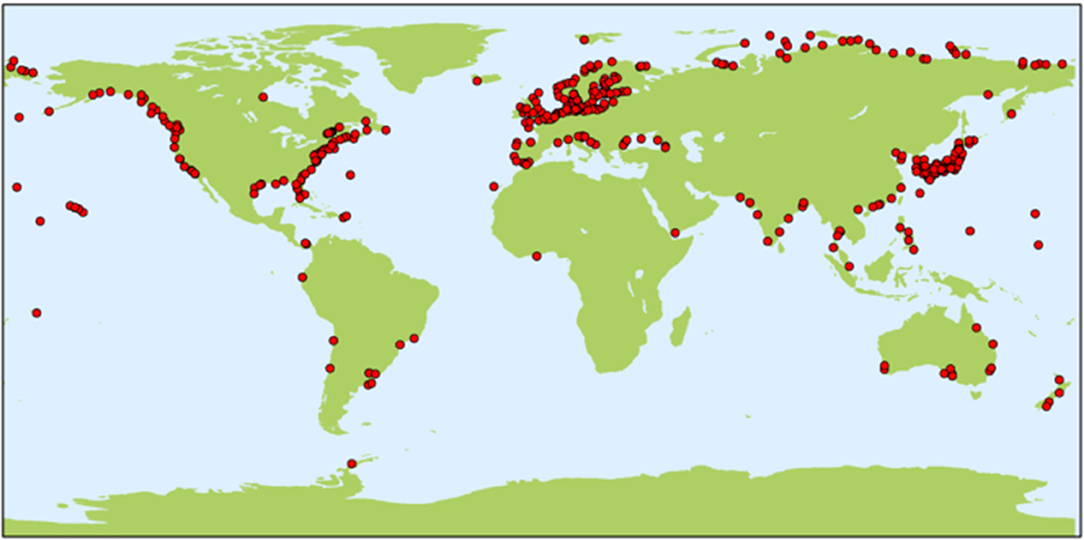
Figure 1. Tide gauge coverage with > 40-year-long records (source: PSMSL; https://www.psmsl.org/products/data_coverage/).

Since the beginning of 1993, sea level is now measured by a succession of altimeter satellites with quasi global coverage. In effect, the launch of the TOPEX/Poseidon mission in August 1992 marked the beginning of the era of high-precision satellite altimetry for applications to oceanography and climate research. The constellation of high-precision satellite altimeters is shown in Figure 2.

FIGURE 2

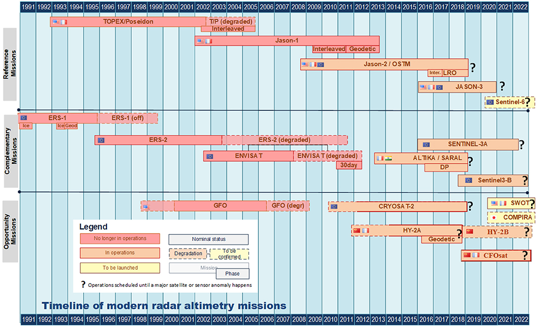
Figure 2. Constellation of high precision altimeter satellites; Status in April 2019.

Outside Europe, several groups routinely process the altimetry data to provide sea level products at global and regional scales. These include:

1) University of Colorado (CU Release 3; http://sealevel.colorado.edu/).

2) Goddard Space Flight Center (GSFC version 2; https://sealevel.jpl.nasa.gov/).

3) National Oceanographic and Atmospheric Administration (NOAA; http://www.star.nesdis.noaa.gov/sod/lsa/SeaLevelRise/LSA_SLR_timeseries_global.php).

4) Commonwealth Scientific and Industrial Research Organization (CSIRO; www.cmar.csiro.au/sealevel/sl_data_cmar.html).

In Europe, altimeter sea level products have been processed by the CNES/CLS DUACS altimeter production system since 2001 (https://duacs.cls.fr) and distributed since 2003 through the AVISO+ CNES Satellite Altimetry Data portal (www.aviso.altimetry.fr/en). Since 2015, the whole processing, operational production and distribution of the DUACS along-track (level 3) and gridded (level 4) altimeter sea level products have been taken over by the European Copernicus Program (with the support of EUMETSAT for Sentinel-3 products). The DUACS production system delivers sea level products for two different Copernicus services:

- The Copernicus Marine Environment Monitoring Service (CMEMS, http://marine.copernicus.eu/): the sea level products focus on the retrieval of mesoscale signals with the best estimate and sampling of the ocean at each moment and are thus dedicated to ocean modeling and ocean circulation analysis. Both delayed-time and near-real-time products are distributed.

- The Copernicus Climate Change Service (C3S, https://climate.copernicus.eu/): the altimeter products focus on the monitoring of the long-term evolution of sea level for climate applications and the analysis of ocean/climate indicators. These delayed-time products have been designed with a focus on homogeneity and stability of the record.

The main differences between the CMEMS and C3S altimeter sea level products concern: (i) the number of altimeters used in the satellite constellation: all available altimeters are considered in the CMEMS products whereas a steady number (two) of altimeters are included in the C3S products; and (ii) the reference field used to compute sea level anomalies: an optimized reference field (mean profiles of sea surface heights) is used for missions with a repetitive orbit in CMEMS whereas an homogeneous mean sea surface is used for all missions in C3S.

All these DUACS altimeter sea level products were previously known as “AVISO” products and should now be called “Copernicus” products. More details on their specification are available in the product user manuals of the respective Copernicus services as well as in Pujol et al. (2016) and Taburet et al. (in press). The AVISO+ portal still includes ocean monitoring indicators (such as the GMSL evolution), added-value and pre-operational research products (https://www.aviso.altimetry.fr/en/data/products/ocean-indicators-products.html).

In addition, from 2011 to 2017, the ESA Sea Level Climate Change Initiative (SL_cci, http://www.esa-sealevel-cci.org/) project has developed new optimized altimeter algorithms that improve the homogeneity and stability of the sea level record. This has led to the production of a delayed-time sea level product including nine altimeter missions and covering the period 1993–2015 (Ablain et al., 2015, 2017a; Quartly et al., 2017; Legeais et al., 2018). The last version of the operational Copernicus sea level products (DT-2018 reprocessing) has benefited from the SL_cci developments. In this context, the operational production of the climate-oriented sea level products by the Copernicus climate service (C3S) extends the sea level time series.

Among the different ocean monitoring indicators, the global mean sea level can either be derived by directly averaging the validated along-track data or averaging gridded data based on optimal interpolation of the along-track data. The long-term stability of the GMSL is ensured by the TOPEX-Poseidon, Jason-1, Jason-2, and Jason-3 reference missions. They are thus essential for the computation of the sea level trends. They cover the ±66° latitude band and have a repeat cycle of 10 days. Other complementary and opportunity missions (ERS-1, ERS-2, Envisat, SARAL/AltiKa, HY-2A, Sentinel-3A & 3B, and CryoSat-2) improve the geographical sampling of mesoscale processes by improving the spatiotemporal resolution, provide high-latitude coverage (up to +/−82°), and increase the sea level accuracy (Figure 3).

FIGURE 3

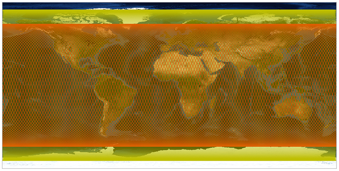
Figure 3. Coverage of high-precision altimetry missions in repeat orbit (red curves correspond to Jason orbits, while yellow curves correspond to Envisat/SARALAltika orbits).

Among the above-listed different international groups that compute the GMSL, each one has its own processing system, considers different satellite missions, applies slightly different geophysical corrections, and has developed different strategies for the data editing and gridding. The GMSL time series derived from the European products (averaging of along-track measurements of the reference missions for AVISO+ and averaging of multi-mission merged gridded CMEMS or C3S products) are considered to be identical since the same altimeter standards are used to compute the sea level anomalies, and the long-term stability is ensured by the same reference missions. The remaining observed GMSL differences are not significant given the uncertainty considered on different scales (Ablain et al., 2015).

The 26-Year-Long Altimetry-Based Global Mean Sea Level

The altimetry-based GMSL record is shown in Figure 4. It is based on the CCI multi-mission merged gridded sea level data up to December 2015 extended with the CMEMS and near-real-time data from Jason-3. The time series is corrected for GIA by subtracting a −0.3 mm/year value from the trend (Peltier, 2004). The seasonal signal is removed by fitting sinusoids of 6- and 12-month periods to the data. The first 6 years of the GMSL record are corrected for an instrumental drift that affects the TOPEX-A altimeter of the TOPEX/Poseidon mission, using the correction proposed by Ablain et al. (2017b). Over the 26-year long time span (January 1993 to February 2019), the mean rate of sea level rise amounts to 3.15 ± 0.3 mm/year, with an acceleration of 0.10 ± 0.04 mm/year² (1-σ errors based on Ablain et al., 2019). This acceleration value agrees well with Nerem et al. (2018)'s estimate, of 0.085 mm/year², after removing the interannual variability of the GMSL.

FIGURE 4

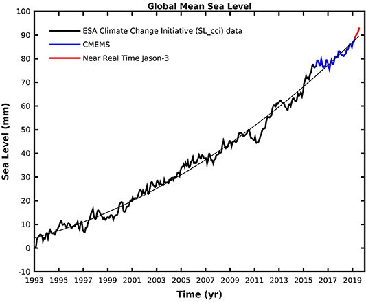
Figure 4. Altimetry-based global mean sea level from January 1993 to February 2019. The black thin solid line is a quadratic function fitted to the data.

Unanswered Scientific Questions and New Challenges in Terms of GMSL Monitoring

To maintain the quality of the altimetry-based sea level record, sustained and ever more accurate observations from space are required. A longer sea level record with increased accuracy (fulfilling the GCOS requirements, GCOS, 2011) will allow addressing unanswered science questions such as: “Does the recently recorded acceleration of sea level rise represent a long-term shift toward a new climate regime? To what amount and over what time scale will potentially abrupt changes in the ice-sheet contributions affect the global sea level? How much heat has already reached the deep ocean? Can we constrain the Earth's energy imbalance and its temporal variations with improved global mean sea level observations? Is the regional variability in sea level only due to internal climate variability or can we already detect the fingerprint of anthropogenic forcing? When should the anthropogenic signal emerge out of the natural variability? Finally, which sectors of the global coastline will be affected first and at the greatest societal cost?” (Cazenave et al., 2019).

At the time of writing, 6 altimetry missions are in orbit (not counting the Chinese missions): Jason-2, Jason-3, SARAL/AltiKa, CryoSat-2, Sentinel-3A, and Sentinel-3B. Two of them (Jason-2 and SARAL/Altika) have been recently placed in non-repeat orbits, similar to the Cryosat-2 mission. However, not all satellites are included when estimating the global mean sea level. For example, NOAA, CU and GSFC only consider the reference missions, and C3S use two satellites (Jason-3 and Sentinel 3A) to extend the CCI time series. In the near future (2020), Sentinel 6 (Jason CS) will be placed on the same orbit as the TOPEX/Poseidon-Jason series. The SWOT mission based on interferometric altimetry technology, to be launched in 2021, will potentially also contribute to the global mean sea level monitoring. The scientific community universally supports the extension of the CryoSat-2 mission beyond 2019. On a longer time frame, the continuation of the radar altimetry record is less clear. Although the Jason and Sentinel satellite series are expected to provide essential sea level measurements over the coming decades for the mid-latitudes, in the Polar Regions—north and south of 82°, which includes the rapidly changing Arctic Ocean—a Polar orbiting cryosphere and ocean observing topography mission is as yet unsecured.

Steric Sea Level

Variations in steric sea level (i.e., due to ocean volume changes that result from density changes linked to temperature and salinity fluctuations) contribute significantly to sea level changes. Although satellite altimeters can measure total sea level change, they are unable to measure steric variability directly. Instead, in situ hydrographic measurements remain critical for sampling the subsurface of the ocean and determining the steric component of the total sea level change measured by satellite altimeters. During most of the Twentieth century, this involved temperature and salinity measurements collected by fixed-point moorings, oceanographic cruises and commercial ships. These data, however, suffer from serious sampling limitations that inhibit the understanding of steric sea level variability. The sampling in space is irregular—tied to ship tracks and fixed buoy locations—and the sampling in time is sporadic and seasonally biased. These issues are exacerbated as the record is extended further into the past, with logistically inaccessible and deeper parts of the ocean particularly undersampled. Furthermore, there is a northern hemisphere and seasonal sampling bias (most data collected during the summer), and remote areas of the global ocean are poorly covered throughout the record and at all depths, with the Southern Ocean one of the gravest cases in terms of data coverage.

During the 1990s, the sampling situation improved significantly with the World Ocean Circulation Experiment (WOCE) project, an international initiative to develop surface and subsurface observing systems that complement satellite-measured sea surface height and sea surface temperature. From this project, a profiling float that could provide measurements of the subsurface of the ocean was developed. This eventually led to the installation of a global array of profiling floats, named Argo, with the primary motivation of assessing climate variability and change, including GMSL change due to steric variations (Roemmich et al., 2012, Riser et al., 2016). The first Argo floats were deployed in 1999, and the global network has included more than 3000 floats since 2007. That number now approaches 4,000 (Figure 5) with 25 national Argo programs around the globe contributing instruments and their deployment. With the data provided by the global array of Argo floats, the steric-related GMSL change has been estimated to be ~1.31 ± 0.5 mm/year (WCRP Global Sea Level Budget Group, 2018) from 2005 to 2015, and a regional map of steric sea level change can be computed with comparable spatial variability to the altimeter-derived trend map over the same time period.

FIGURE 5

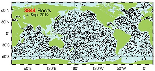
Figure 5. Coverage of the global ocean by Argo floats on 04 September 2019.

Despite the significant advances that have been made as a result of the Argo sampling program, observational needs remain with respect to improving our understanding of steric sea level change. The most prominently used Argo floats sample only to a depth of 2,000 m, limiting our understanding of the changes that may be occurring at depth layers below. Such changes would be reflected in the total sea level observations from satellite altimeters, which creates a gap in sea level budget calculations that rely on Argo for the steric contribution. Recent advances in profiling float and sensor technologies have led to the development of profiling floats that can sample to depths of 6,000 m (Zilberman, 2017). Regional pilot arrays are already in place in the Southwest Pacific Basin, South Australian Basin, Australian Antarctic Basin, and North Atlantic Ocean, and it is critical that a transition to full-depth global ocean observation continues to occur over the coming years. Additionally, even with the dramatic improvement in sampling with Argo profiling floats, there are still areas of the ocean that are undersampled, with marginal seas, shallow shelf areas, and seasonally ice-covered oceans among the most notable and scientifically important of these areas (Von Schuckmann et al., 2016). During early stages of Argo, the decision was made to avoid deployments in many marginal seas due to the risk of premature loss of floats and potentially problematic political issues. Since then, efforts have been made to encourage deployments in such areas, but as seen in Figure 5, areas like the Southeast Asian Seas (SEAS) remain very poorly covered. Variability in the SEAS region can have a substantial impact on global sea level and on heat storage on interannual timescales, making them critical to observe. Finally, coverage in areas poleward of 60 degrees North and South remains poor due to low deployment and high rates of attrition associated with the presence of sea ice floes that can damage the floats. Technological advances have been made that allow for ice avoidance of the floats, with increased lifetimes shown for these adapted floats. Increasing the deployment of ice-adapted floats would provide an improved understanding of sea level change at both global and regional scales.

Mass Contributions

Mass changes and redistributions in the Earth system, notably redistribution of water (in its liquid, solid, or gaseous state), can be observed through their gravitational effect by satellite gravimetry missions. GRACE was a joint mission by NASA and DLR (the German Aerospace Center) which operated from 2002 to 2017. The mission concept built on the sensitivity of the orbits of low Earth orbiting satellites to the spatial details of the Earth's gravitational field. GRACE consisted of two satellites following each other in a distance of 200 km in a near-polar orbit. Variations in the distance between the two satellites, which are related to variations in the gravitational attraction of the Earth's mass, were measured by a K-band microwave ranging system with micrometer precision. A GPS tracking system for orbit determination, star cameras used for attitude determination and control and a 3D accelerometer for the measurement of non-gravitational accelerations were among the instruments completing the system. Based on the measurements, the global gravity field was solved for, typically on a monthly basis. The temporal variations of the monthly gravity field solutions were then analyzed to infer temporal changes in the mass of elements in the Earth system. GRACE is now followed by the GRACE-Follow-On (GRACE-FO) mission launched in May 2018 (https://gracefo.jpl.nasa.gov, https://www.gfz-potsdam.de/en/section/global-geomonitoring-and-gravity-field/projects/gravity-recovery-and-climate-experiment-follow-on-grace-fo-mission) with essentially the same mission configuration complemented by an even more precise laser ranging system between the twin satellites.

Satellite gravimetry is unique because it is directly sensitive to mass changes (rather than volume changes), including mass changes of the global ocean (Johnson and Chambers, 2013, Chen et al., 2013, Rietbroek et al., 2016). GRACE has enabled the “golden era” of sea level budget assessments where ocean mass change can be directly determined to complement the determination of volume change by altimetry and the determination of density change by the Argo sensor system. The WCRP study on global sea level budget (WCRP Global Sea Level Budget Group, 2018) provides a survey on recent GRACE-based ocean mass change studies and results (Figure 6).

FIGURE 6

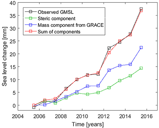
Figure 6. The sea level budget over the golden era, using GRACE-based estimates of ocean mass change. The ensemble mean annual time series published by WCRP Global Sea Level Budget Group (2018) are shown.

Global mean ocean mass change may also be considered by assessing the individual contributions from mass changes of ice, snow, and water mass on land. Apart from the use of satellite gravimetry to determine these mass changes (discussed later), there are established approaches for such assessments for each land water/land ice storage component. The mass balance of the Antarctic and Greenland Ice Sheets can been estimated using a temporally continuous record of ice volume change measured by satellite altimetry missions since 1992, combined with an estimate of the density at which these changes occurred (Wingham et al., 1998; Shepherd et al., 2012, 2018; McMillan et al., 2014; Sørensen et al., 2018). Alternatively, the difference between surface mass balance into the basin estimated by a regional climate model (snow accumulation minus ablation), satellite observations of ice discharge out of the basin measured using InSAR or optical satellite data, and an estimate of the ice thickness across a flux gate, can be used to compute mass balance using the Input Output Method (IOM) (Mouginot et al., 2014). Mass changes of the world's mountain glaciers and ice caps have been estimated from the spatial extrapolation of field observations that are based on the direct or glaciological method for selected glaciers globally (e.g., Dyurgerov and Meier, 1997; Kaser et al., 2006) or later in combination with measurements based on the geodetic method, i.e., differencing of DEMs from at least two points in time (Cogley, 2009). More recently, the direct measurements have been used in conjunction with global-scale glacier modeling to infer their contribution forward (e.g., Radic and Hock, 2011) and backward in time (e.g., Marzeion et al., 2012). Another global-scale assessment of glacier mass change over the 2003–2009 period by Gardner et al. (2013) combined results from the glaciological method with trends in elevation derived from ICESat and gravimetric information from GRACE. Changes of the global continental water storage (including snow cover) at decadal (due mainly to groundwater depletion and man-made reservoirs) and seasonal scales have been assessed from global hydrological modeling (Döll et al., 2014a,b; Wada et al., 2017; Scanlon et al., 2018). In global hydrological modeling, a multitude of data including storage capacities of man-made reservoirs and the area of irrigated cropland are taken into account.

Satellite gravimetry has not only enabled the estimation of ocean mass change itself but has also added a powerful means of assessing its continental sources. GRACE has become instrumental in recording ice sheet mass change (Velicogna and Wahr, 2006, Horwath and Dietrich, 2009), in validating global hydrological modeling results (Döll et al., 2014a; Scanlon et al., 2018), and also in estimating mass losses of the world's glaciers and ice caps (Luthcke et al., 2008, Jacob et al., 2012, Gardner et al., 2013). By weighing mass changes in the Earth system due to whatever contributory process in an integrative, globally consistent way, satellite gravimetry has become the overarching technique for assessing the ocean mass budget.

Current limitations of satellite gravimetry can be summarized in four categories: (a) the limited temporal coverage, (b) the limited spatial resolution, (c) the problem of separating superimposed signals of mass change, including the GIA effects, and (d) the insensitivity to mass redistributions of spherical harmonic degree one (the so-called geocenter motion). These limitations directly translate into observational requirements for the future and will be discussed in the following.

(a) GRACE, originally designed for a 5-year lifetime, operated from 2002 through 2017, with some degradation of instruments and data recovery in the late years of the mission. Fortunately, GRACE-FO was launched in 2018, so that only a moderate gap occurred between the two missions. Since both missions determine the global gravity field in an absolute sense, no inter-mission calibration issues are expected. However, a long-term commitment to satellite gravimetry missions as a core element of Earth observation is not yet established by any organization. An essential observational requirement therefore consists in the continuation and operationalization of satellite gravimetry missions, following the example of, and complementing, satellite altimetry missions or meteorological missions. Recently, the National Research Council of the United States National Academies of Sciences, Engineering, and Medicine published the Decadal Strategy for Earth Observation from Space [Decadal Survey, NRC (National Research Council, The National Academies of Sciences, Engineering, and Medicine), 2018], where mass change was identified as one of the top 5 observables to be implemented by future US Earth observation missions in order to ensure continuity and enable long-term mass budget analyses of the Earth system.

(b) The attenuation of gravity field signals of small spatial scale at satellite height causes a decreasing sensitivity of satellite gravimetry to small spatial scales. In other words, the spatial resolution of GRACE-based mass change inferences is coarse, unless the inferences are guided by additional a-priori information. The signal-to-noise ratio of GRACE-based mass changes decreases to less than one for spatial scales smaller than 200–500 km, depending on signal strength, time scale, and latitude. In addition, the GRACE (and GRACE-FO) orbital geometry in conjunction with deficiencies in modeling short-term mass variations induces distinctly anisotropic error characteristics reflected in north-south striping of unregularized solutions. The limits in spatial resolution lead to so-called leakage effects in attributing observed gravity field changes to the geographic location of the underlying mass changes. For the example of ocean mass budget applications, leakage effects manifest themselves in the difficulty of attributing an increase of gravitational attraction in the vicinity of coastlines to either regional ocean mass increase or regional continental water/ice mass increase, that is, to either a positive or a negative contribution to the ocean mass budget. The limited spatial resolution also prevents the detection of regional patterns of ocean mass change in a spatial resolution comparable to that of altimetry results and steric results.

New mission concepts with improved instrumentation and different satellite orbit constellations as well as improved modeling of background signals and improved processing strategies are means of increasing the spatial resolution of satellite gravimetry. In a community effort, Pail et al. (2015a,b) identified threshold and target scenarios for future satellite gravity missions, including the consideration of oceanographic and ocean mass change requirements. To meet these demands, currently several concepts for Next-Generation Gravity Missions (NGGMs) are under investigation and discussion. These concepts are usually based on high-precision inter-satellite ranging observations but differ in the set-up of the satellite constellation and the resulting observation geometry. In 2013 the mission concept called “e.motion” was proposed in response to ESA's Earth Explorer (EE) Call 8 (Panet et al., 2013). It was based on a pair of low-flying satellites in a so-called pendulum orbit, where the trailing satellite performs a relative pendulum motion behind the leading one. As another promising constellation, double-pairs in Bender configuration (Bender et al., 2008) consist of two GRACE/GRACE-FO-like pairs, where one pair flies in a (near-)polar orbit and the other one in an inclined orbit of 60° to 70°. This configuration significantly reduces the typical striping error patterns of GRACE and GRACE-FO temporal gravity solutions (Wiese and Visser, 2011; Daras and Pail, 2017). The EE9 proposal e.motion² (Gruber et al., 2015) was based on the idea of a Bender double pair. Another promising constellation is high-precision tracking between high or medium orbiting and low orbiting satellites (Hauk et al., 2017). The observation geometry, which is mainly in radial direction, results in a significant reduction of striping effects. It was the basis for the gravity mission proposal called “MOBILE” in response to the ESA EE Call 10 (Hauk and Pail, 2019).

(c) While the horizontal resolution of satellite gravimetry can be improved by refinement and extension of mission concepts, the inability of gravimetry to separate vertically superimposed signals of mass changes is a mathematical fact. While the separation of atmospheric mass changes is routinely conducted by use of atmospheric modeling, the separation of mass redistribution in the Earth's interior due to GIA from long-term redistribution of water and ice masses on the Earth surface constitutes a major source of uncertainty for GRACE-based ocean mass changes as well as GRACE-based mass contributions from the Antarctic Ice Sheet. The common way of accounting for GIA is to use geophysical GIA modeling results, which in turn rely on assumptions on glaciation history and Earth rheology (Spada, 2017; Whitehouse, 2018). The difference between global ocean mass change obtained when applying different global GIA models is on the order of 0.2 mm/year mean sea level (e.g., Blazquez et al., 2018). An additional complication arises from the fact that Antarctic ice sheet applications of GRACE have used regional GIA models, which are different from, and inconsistent with, global GIA models because global GIA models are considered incompatible with regional geological evidence on Antarctic glacial history (Ivins et al., 2013). Apart from improving geophysical GIA modeling by using the growing body of geological and geodetic constraints on sea level and glaciation history and by accounting for lateral variations of Earth rheology and non-Maxwell rheologies, it appears that geodetic observations of GIA, in particular GNSS observations of Earth surface deformations in Antarctica and Greenland, are a critical observational requirement for constraining ocean mass change and the ocean mass budget (King et al., 2010, Groh et al., 2012, Khan et al., 2016, Barletta et al., 2018). Satellite remote sensing by synthetic aperture radar has the potential of adding complementary, spatially extended information to the pointwise GNSS measurements (Auriac et al., 2013, Yan et al., 2016). Any development to observe bedrock deformations below ice sheets with a millimeter-per-year precision would fill crucial gaps in Antarctic GIA observation.

(d) Satellite gravimetry missions are insensitive to the largest spatial scale of water and ice mass redistribution, namely to the spherical harmonic components of degree one. Roughly speaking, degree-one patterns reflect a net mass exchanges between hemispheres, or in other words, a shift of the center of mass of the considered water and ice masses. The problem is directly linked to the determination of geocenter motion and thereby to the realization of the global terrestrial reference system origin and of the transformation between different origin definitions (Wu et al., 2012). Swenson et al. (2008) inferred degree-one components from a combination of GRACE-based gravity field variations with model-based assumptions on the water redistribution in the global ocean. This approach has been widely used with different modifications. However, with this approach the inferences on ocean mass change and ocean mass redistribution are inherently dependent on a priori assumptions about the same processes. The geodetic space techniques used to realize global terrestrial reference systems, in particular Satellite Laser Ranging, are capable of determining geocenter motion independently. It is of utmost importance to maintain and further develop the related global geodetic infrastructure and data analysis capacities. The International Association of Geodesy promotes this development by its Global Geodetic Observing System, and the United Nations (UN) have emphasized the importance by the resolution “Global Geodetic Reference Frame for Sustainable Development” (U. N. United Nations General Assembly, 2015; U. N. United Nations, 2016). The geodetic infrastructure related to the global reference frame realization forms the observational backbone for both the gravimetric determination of ocean mass changes and the geometric observation of sea level change by satellite altimetry, since the altimeter satellites' orbit determination crucially depends on reference frame realization.

The detailed assessment of the sources of ocean mass change in continental water and ice mass changes calls for further developments of their specific observation techniques and systems.

For the Greenland and Antarctic ice sheets, mass balance assessments will benefit from the ongoing and respective developments of satellite and airborne remote sensing, such as high-resolution and high-accuracy observations of surface elevation change from satellite altimeters with advanced resolution capability such as CryoSat-2, Sentinel-3, and ICESat-2, operational ice velocity mapping by imaging sensors such as Sentinel-1, Sentinel-2 and Landsat, ice thickness measurements by ground-penetrating radar to support assessments of discharge by ice flow, or firn radar measurements to support assessments of surface mass balance and firn processes. The mentioned techniques and missions need to be continued and further developed.

All estimates of glacier mass loss critically depend on the availability of a precise glacier inventory. Only with the availability of the Randolph Glacier Inventory in 2012 (Pfeffer et al., 2014) could the related global-scale calculations be performed with some certainty. Considering the rapid glacier shrinkage globally, a long-term strategy for monitoring global sea level has thus to ensure regular updates of the global glacier inventory (GCOS, 2011). Another obvious requirement concerns the information on glacier changes through time. Whereas field observations contribute direct measurements of annual or seasonal mass changes on the selected glaciers globally (Zemp et al., 2015), remote sensing data provide complementary information on glacier extent (from optical sensors), elevation changes (from repeat altimetry or Digital Elevation Model–DEM- differencing), and velocity to determine the mass flux for calving glaciers (from optical and microwave sensors). Well-established processing lines (Paul et al., 2015) provide these datasets from the fleet of currently available optical (e.g., Landsat, Sentinel-2, ASTER), microwave (e.g., Sentinel-1, ALOS PALSAR, TerraSAR-X/TanDEM-X), and altimetry sensors (e.g., ICESat-2, Cryosat-2), which need to be continued. Key technical issues to be addressed for improved geodetic mass balances are radar penetration for DEMs derived from microwave sensors (SRTM and TanDEM-X) and handling of data voids and artifacts over glaciers that are common in all DEMs (e.g., McNabb et al., 2019). There is also a requirement for the availability of DEMs, to update such DEMs frequently (e.g., every ten years), to provide them with a clear timestamp, and to improve constantly their quality and spatial resolution.

Estimation of land water storage changes (including snow) by global hydrological models can be improved in the future by data assimilation of multiple observational variables into global hydrological models (Döll et al., 2016). These observations include, in addition to in situ observations of streamflow, geodetic, and remote-sensing time series of total water storage anomalies from satellite gravimetry and GNSS, water table variations of surface water bodies and the extent of surface water bodies and snow. Of particular importance are more accurate global digital elevation models as well as remote-sensing-based stream flow estimates. Where access is possible, the water table elevation-streamflow relation could be determined first by an in situ measurement, which would allow translating radar altimetry measurements of water table elevations, ideally once per day, to streamflow time series.

The benefit from observational developments specific to the individual ocean mass sources discussed above will ultimately depend on the ability to consistently combine the observation systems for each individual element of the ocean mass budget and finally for the ocean mass budget and sea level budget as a whole. Pioneering examples include the combination of satellite altimetry, satellite gravimetry and GNSS to separate ice sheet mass changes and GIA (Riva et al., 2009; Gunter et al., 2014; Martín-Español et al., 2016; Sasgen et al., 2017) or integrating global geometric and gravimetric observations in global inversions for sea level changes and their contributions (Rietbroek et al., 2016).

Integration

By nature, the global mean sea level budget is an integrative topic. It combines different ECVs that are derived from totally independent observing systems. These include satellite altimetry, GRACE space gravimetry, in situ measurements of temperature and salinity from ships and Argo floats as well as outputs from various models.

As reported in recent publications, near closure of the sea level budget over the altimetry era indicates that no serious systematic errors currently affect these observing systems (at the level of 0.3 mm/year in terms of sea level trend equivalent). It also provides cross calibration of the systems.

Integrative analyses performed to examine closure of the sea level budget also inform on the level of uncertainty of each component, thus calling for additional research on adjacent topics. For example, uncertainty on the land water component derived from the budget analysis may question the quality of the meteorological forcing used to run the hydrological models. The level of closure also informs on missing components, e.g., deep ocean warming below 2,000 m not sampled by Argo, providing constraints on the current Earth energy imbalance (another important climate issue).

User Engagement

The primary users of the GMSL record and of the sea level budget are meteorological and climate organizations. The WMO now integrates the sea level ECV and the sea level budget in its yearly reports on the State of the Global Climate (WMO (World Climate Organization), 2019). The data sets for the GMSL already feed the “OBS4MIP” database of the WCRP. Data sets for the components of the sea level budget should also be included in OBS4MIP in the future. This will be most useful for CMIP (Climate Model Intercomparison Project) exercises, including coupled climate model validation. The IPCC (Intergovernmental Panel on Climate Change) reports are the ultimate users of this process.

In addition to these institutional users, public and private stakeholders are mostly interested in gaining information about GMSL changes. Although it is a slow process, sea level rise counts among the most ominous impacts of current climate change. It is one of the most pressing societal threats. Sea level rise at the coast results from several contributions: the global mean sea level rise, the superimposed regional variability, and the small-scale coastal processes. On the long term (several decades), the global mean rise will dominate the other factors. To assess present-day and future coastal risks (e.g., temporary and permanent flooding at the coast, shoreline retreat, etc.), national and regional authorities in charge of developing adaptation strategies to cope with climate change impacts, including sea level rise, represent a new category of end users that need to be regularly informed on the state of the climate and its future evolution. Novel procedures of communication toward the civil society, governmental organizations, and the private sector should be implemented so that the most up-to-date climate-related information, including the rate of sea level rise (present and future) and its causes (hence the sea level budget), can be regularly delivered outside the science community, in support of societal needs.

Conclusions and Recommendations

To assess the global mean sea level budget, i.e., we need sustained observations with as global as possible coverage of sea level by satellite altimetry and of the steric and mass components from various space-based and in situ observing systems.

For sea level, we recommend:

- Continuity of the high-precision altimetry record beyond Sentinel-6/Jason-CS,

- Investigation of the possibility to modify the orbital characteristics of the reference missions in order to cover the Arctic Ocean,

- Maintain the level of quality of the historical past missions as high as possible (through regular data reprocessing) to ensure the homogeneity of the time series,

- Maintain the sea level measurements at high latitudes with the continuity of the CryoSat-2 mission.

For the steric component, priorities are (see also Meyssignac et al., 2019, this issue):

- Maintain support for Core Argo (www.argo.ucsd.edu, doi: 10.17882/42182),

- Implement Deep Argo,

- Perform regular subsurface temperature measurements (e.g., using dedicated Argo floats or other autonomous devices, and ship measurements) in areas not well-covered: marginal seas, high latitudes, boundary currents, and shallow areas and shelf regions,

- Perform/assure systematic calibration of Argo measurements using independent observing systems, notably the maintenance of CTD (conductivity/temperature/depth) shipboard measurements used for the quality control procedure for Argo measurements; assure development of these calibration values in-line with extensions of Argo (e.g., assure deep shipboard profiles for deep Argo).

For the mass component, recommendations include:

- Sustained measurements of ocean mass changes, of ice sheet and glaciers mass balances, and of land water storage changes from a GRACE-type mission with improved performances, especially in terms of spatial resolution,

- Sustained monitoring of land ice bodies using various remote sensing systems (InSAR, radar and optical imagery, standard radar as well as SAR/SARIN, and laser altimetry) and modeling,

- Improvement of global hydrological models, which requires, in particular, more accurate global digital elevation models as well as remote-sensing-based stream flow estimates.

In addition to observational requirements, we also recommend continuing modeling efforts for terms to consider in the global mean sea level budget but not yet easily accessible by observations. This includes improvement of GIA models.

Notwithstanding, reducing errors still affecting all terms of the sea level budget remains a major goal. Most recent studies of the global mean sea level budget find closure of the budget to about 0.2–0.3 mm/year in terms of trend, the attached uncertainty being on the order of 0.3 mm/year. This uncertainty level of 0.3 mm/year (of the same order of magnitude as some components; e.g., land water storage, GIA) looks to be a threshold that appears difficult to overcome. Moreover, this 0.3 mm/year uncertainty does not account for systematic errors affecting each term of the budget. For example, the GMSL trend (systematic) uncertainty is estimated to 0.3–0.4 mm/year (Legeais et al., 2018, Nerem et al., 2018). Errors of the wet tropospheric correction applied to the altimetry data and link between successive missions remain the largest contributors to the GMSL trend uncertainty (Ablain et al., 2019). Additional errors come from the Terrestrial Reference Frame in which the altimeter measurements are represented. A space geodetic collocation experiment—GRASP (Geodetic Reference Antenna in SPace)—has been proposed to reduce some of these reference frame uncertainties by tying together the major geodetic techniques (GNSS, SLR, DORIS, and VLBI). More work is needed to understand the remaining systematic errors of each term of the budget and reduce them.

Author's Note

In response to the OCEANOBS19 call for future observing systems of the ocean, the first three authors submitted community white paper abstracts dedicated to the sea level budget. They were further invited to group together to prepare a single merged article. This manuscript is the outcome of such a merging.

Author Contributions

AC, BH, and MH wrote the manuscript, benefitting from input and improvement from all co-authors. All co-authors contributed to the paper.

Conflict of Interest Statement

The authors declare that the research was conducted in the absence of any commercial or financial relationships that could be construed as a potential conflict of interest.

The reviewer HD declared a shared affiliation with several of the authors, AC, BM, and HP, and a past collaboration with one of the authors, AC, to the handling editor at time of review. The peer review was handled under the close supervision of the Chief Editor to ensure an objective process.

Acknowledgments

We thank the two reviewers for their comments that helped us to improve the manuscript.

References

Ablain, M., Cazenave, A., Larnicol, G., Balmaseda, M., Cipollini, P., Faugère, Y., et al. (2015). Improved sea level record over the satellite altimetry era (1993–2010) from the Climate Change Initiative project. Ocean Sci. 11, 67–82. doi: 10.5194/os-11-67-2015

CrossRef Full Text | Google Scholar

Ablain, M., Jugier, R., Zawadki, L., Taburet, N., Cazenave, A., Meyssignac, B., et al. (2017b). The TOPEX-A Drift and Impacts on GMSL Time Series. AVISO Website. Available online at: https://meetings.aviso.altimetry.fr/fileadmin/user_upload/tx_ausyclsseminar/files/Poster_OSTST17_GMSL_Drift_TOPEX-A.pdf.

Google Scholar

Ablain, M., Legeais, J. F., Prandi, P., Marcos, M., Fenoglio-Marc, L., Benveniste, J., et al. (2017a). Satellite altimetry-based sea level at global and regional scales. Surv. Geophys. 38, 7–31. doi: 10.1007/s10712-016-9389-8

CrossRef Full Text | Google Scholar

Ablain, M., Meyssignac, B., Zawadski, L., Jugier, R., Ribes, A., Cazenave, A., et al. (2019). Uncertainty in satellite estimate of Global mean Sea level changes, trend and acceleration. Earth Syst. Sci. Data. 11, 1189–1202. doi: 10.5194/essd-2019-10

CrossRef Full Text | Google Scholar

Auriac, A., Spaans, K. H., Sigmundsson, F., Hooper, A., Schmidt, P., and Lund, B. (2013). Iceland rising: Solid Earth response to ice retreat inferred from satellite radar interferometry and visocelastic modeling. J. Geophys. Res. 118, 1331–1344. doi: 10.1002/jgrb.50082

CrossRef Full Text | Google Scholar

Bamber, J., and Riva, R. (2010). The sea level fingerprint of recent ice mass fluxes. Cryosphere 4, 621–627. doi: 10.5194/tc-4-621-2010

CrossRef Full Text | Google Scholar

Barletta, V. R., Bevis, M., Smith, B. E., Wilson, T., Brown, A., Bordoni, A., et al. (2018). Observed rapid bedrock uplift in Amundsen Sea Embayment promotes ice-sheet stability. Science 360, 1335–1339. doi: 10.1126/science.aao1447

PubMed Abstract | CrossRef Full Text | Google Scholar

Bender, P. L., Wiese, D. N., and Nerem, R. S. (2008). “A possible Dual-GRACE mission with 90 degree and 63 degree inclination orbits,” in Proceedings of the 3rd International Symposium on Formation Flying, Missions and Technologies. European Space Agency Symposium Proceedings, SP-654 jILA Pub. 8161 (Noordwijk).

Google Scholar

Benveniste, J., Cazenave, A., Vignudelli, S., Fenoglio Marc, L., Shah, R., Almar, R., et al. (2019). Requirements for a Coastal Hazard Observing System. Front. Mar. Sci. 6:348. doi: 10.3389/fmars.2019.00348

CrossRef Full Text | Google Scholar

Blazquez, A., Meyssignac, B., Lemoine, J. M., Berthier, E., Ribes, A., and Cazenave, A. (2018). Exploring the uncertainty in GRACE estimates of the mass redistributions at the Earth surface: implications for the global water and sea level budgets. Geophys. J. Int. 215, 415–430. doi: 10.1093/gji/ggy293

CrossRef Full Text | Google Scholar

Cazenave, A., Guinehut, S., Ramillien, G., Berthier, E., Llovel, W., Ramillien, G., et al. (2009).Sea level budget over 2003-2008; a reevalution from satellite altimetry, GRACE and Argo data. Glob. Planet. Change. 65, 83–88. doi: 10.1016/j.gloplacha.2008.10.004

CrossRef Full Text | Google Scholar

Cazenave, A., Meehl, G., Montoya, M., Toggweiler, J. R., and Claudia Wieners, C. (2019). “Climate change and impacts on variability and interactions,” in Interacting Ocean Climates: Observations, Mechanisms, Predictability, and Impacts, ed R. Mechoso (Cambridge University Press).

Google Scholar

Chambers, D. P., Cazenave, A., Champollion, N., Dieng, H., Llovel, W., Forsberg, R., et al. (2017). Evaluation of the Global Mean Sea Level Budget between 1993 and 2014. Surv. Geophys. 38, 309–327. doi: 10.1007/s10712-016-9381-3

CrossRef Full Text | Google Scholar

Chen, J. L., Wilson, C. R., and Tapley, B. D. (2013). Contribution of ice sheet and mountain glacier melt to recent sea level rise. Nat. Geosci. 6, 549. doi: 10.1038/ngeo1829

CrossRef Full Text | Google Scholar

Chen, X., Zhang, X., Church, J. A., watson, C. S., King, M. A., Monselesan, D., et al. (2017). The increasing rate of global mean sea-level rise during 1993–2014. Nat. Clim. Change 7, 492–495. doi: 10.1038/nclimate3325

CrossRef Full Text | Google Scholar

Church, J. A., Clark, P. U., Cazenave, A., Gregory, J. M., Jevrejeva, S., Levermann, A., et al. (2013). “Sea level change,” in Climate Change 2013: The Physical Science Basis. Contribution of Working Group I to the Fifth Assessment Report of the Intergovernmental Panel on Climate Change, eds T. F. Stocker, D. Qin, G.-K. Plattner, M. Tignor, S.K. Allen, J. Boschung, et al. (Cambridge; New York, NY: Cambridge University Pres).

Google Scholar

Church, J. A., and White, N. J. (2011). Sea-Level Rise from the Late 19th to the Early 21st Century. Surv. Geophys. 32, 585–602. doi: 10.1007/s10712-011-9119-1

CrossRef Full Text | Google Scholar

Cogley, J. G. (2009). Geodetic and direct mass-balance measurements: comparison and joint analysis. Ann. Glaciol. 50, 96–100. doi: 10.3189/172756409787769744

CrossRef Full Text | Google Scholar

Dangendorf, S., Marcos, M., Wöppelmann, G., Conrad, C. P., Frederikse, T., and Riva, R. (2017). “Reassessment of 20th Century global mean sea level rise,” in Proceedings of the National Academy of Sciences, Vol. 114, 5946–5951. doi: 10.1073/pnas.1616007114

CrossRef Full Text | Google Scholar

Daras, I., and Pail, R. (2017): Treatment of temporal aliasing effects in the context of next generation satellite gravimetry missions. J. Geophys. Res. 122, 7343–7362. doi: 10.1002/2017JB014250.

CrossRef Full Text | Google Scholar

Dieng, H. B., Cazenave, A., Meyssignac, B., and Michaël, A. (2017). New estimate of the current rate of sea level rise from a sea level budget approach. Geophys. Res. Lett. 44. doi: 10.1002/2017GL073308

CrossRef Full Text | Google Scholar

Döll, P., Douville, H., Güntner, A., Müller Schmied, H., and Wada, Y. (2016): Modelling freshwater resources at the global scale: challenges prospects. Surve. Geophys. 37, 195–221. doi: 10.1007/s10712-015-9343-1

CrossRef Full Text | Google Scholar

Döll, P., Fritsche, M., Eicker, A., and Schmied, H. M. (2014a). Seasonal water storage variations as impacted by water abstractions: comparing the output of a global hydrological model with GRACE and GPS observations. Surv. Geophys. 35, 1311–1331. doi: 10.1007/s10712-014-9282-2

CrossRef Full Text | Google Scholar

Döll, P., Müller Schmied, H., Schuh, C., Portmann, F., and Eicker, A. (2014b): Global-scale assessment of groundwater depletion related groundwater abstractions: combining hydrological modeling with information from well observations GRACE satellites. Water Resour. Res. 50, 5698–5720. doi: 10.1002/2014WR015595

CrossRef Full Text | Google Scholar

Dyurgerov, M. B., and Meier, M. F. (1997). Mass balance of mountain and subpolar glaciers: a new global assessment for 1961–1990. Arctic Alpine Res. 29, 379–391. doi: 10.2307/1551986

CrossRef Full Text | Google Scholar

Gardner, A. S., Moholdt, G., Cogley, J. G., Wouters, B., Arendt, A. A., Wahr, J., et al. (2013). A reconciled estimate of glacier contributions to sea level rise: 2003 to 2009. Science 340, 852–857. doi: 10.1126/science.1234532

PubMed Abstract | CrossRef Full Text | Google Scholar

GCOS (Global Climate Observing System) (2011). Systematic Observation Requirements for Satellite-Based Data Products for Climate (2011 Update) – Supplemental Details to the Satellite-Based Component of the “Implementation Plan for the Global Observing System for Climate in Support of the UNFCCC (2010 Update)”, GCOS-154 (WMO). Available online at: https://library.wmo.int/opac/doc_num.php?explnum_id = 3710 (accessed: August 10, 2017).

Google Scholar

Groh, A., Ewert, H., Scheinert, M., Fritsche, M., Rülke, A., Richter, A., et al. (2012). An investigation of glacial isostatic adjustment over the Amundsen Sea sector, West Antarctica. Glob. Planet. Change 98, 45–53. doi: 10.1016/j.gloplacha.2012.08.001

CrossRef Full Text | Google Scholar

Gruber, T., Panet, I., and e.motion2 Team (2015). Proposal to ESA's Earth Explorer Call 9: Earth System Mass Transport Mission – e.motion2, Deutsche Geodätische Kommission der Bayerischen Akademie der Wissenschaften, Reihe B, Angewandte Geodäsie, Series B. Available online at: https://dgk.badw.de/fileadmin/user_upload/Files/DGK/docs/b-318.pdf.

Google Scholar

Gunter, B. C., Didova, O., Riva, R. E. M., Ligtenberg, S. R. M., Lenaerts, J. T. M., King, M. A., et al. (2014). Empirical estimation of present-day Antarctic glacial isostatic adjustment and ice mass change. Cryosphere 8, 743–760. doi: 10.5194/tc-8-743-2014

CrossRef Full Text | Google Scholar

Hauk, M., and Pail, R. (2019). Gravity field recovery by high-precision high-low inter-satellite links. Remote Sensing 2019, 11(5), 537; https://doi.org/10.3390/rs11050537.

Google Scholar

Hauk, M., Schlicht, A., Pail, R., and Murböck, M. (2017): Gravity field recovery in the framework of a Geodesy Time Reference in Space (GETRIS). Adv. Space Res. 59, 2032–2047. doi: 10.1016/j.asr.2017.01.028

CrossRef Full Text | Google Scholar

Hay, C. C., Morrow, E., Kopp, R. E., and Mitrovica, J. X. (2015). Probabilistic reanalysis of twentieth-century sea-level rise. Nature 517, 481–484. doi: 10.1038/nature14093

PubMed Abstract | CrossRef Full Text | Google Scholar

Horwath, M., and Dietrich, R. (2009). Signal and error in mass change inferences from GRACE: the case of Antarctica. Geophys. J. Int. 177, 849–864. doi: 10.1111/j.1365-246X.2009.04139.x

CrossRef Full Text | Google Scholar

Horwath, M., Novotny, K., Cazenave, A., Palanisamy, H., Marzeion, B., Paul, F., et al. (2018). ESA Climate Change Initiative (CCI) Sea Level Budget Closure (SLBC_cci) Sea Level Budget Closure Assessment Report D3.1. Version 1.0, 2018. Available online at: https://www.researchgate.net/publication/324170685_Global_sea_level_budget_and_ocean_mass_budget_assessment_initial_results_from_ESA%27s_CCI_Sea_Level_Budget_project.

Google Scholar

Ivins, E., James, T. S., Wahr, J., Schrama, E. J. O., Landerer, F. W., and Simon, K. M. (2013). Antarctic Contribution to Sea-level Rise Observed by GRACE with Improved GIA Correction. J. Geophys. Res. 118, 3126–3141. doi: 10.1002/jgrb.50208

CrossRef Full Text | Google Scholar

Jacob, T., Wahr, J., Pfeffer, W. T., and Swenson, S. (2012). Recent contributions of glaciers and ice caps to sea level rise. Nature 482, 514–518. doi: 10.1038/nature10847

PubMed Abstract | CrossRef Full Text | Google Scholar

Jevrejeva, S., Moore, J. C., Grinsted, A., Matthews, A. P., and Spada, G. (2014). Trends and acceleration in global and regional sea levels since 1807. Glob. Planet. Change 113, 11–22. doi: 10.1016/j.gloplacha.2013.12.004

CrossRef Full Text | Google Scholar

Johnson, G. C., and Chambers, D. P. (2013). Ocean bottom pressure seasonal cycles and decadal trends from GRACE Release-05: Ocean circulation implications. J. Geophys. Res. 118, 4228–4240. doi: 10.1002/jgrc.20307

CrossRef Full Text | Google Scholar

Kaser, G., Cogley, J. G., Dyurgerov, M. B., Meier, M. F., and Ohmura, A. (2006). Mass balance of glaciers and ice caps: consensus estimates for 1961–2004. Geophys. Res. Lett. 33. doi: 10.1029/2006GL027511

CrossRef Full Text | Google Scholar

Khan, S. A., Sasgen, I., Bevis, M., van Dam, T., Bamber, J. L., Wahr, J., et al. (2016). Geodetic measurements reveal similarities between post–Last Glacial Maximum and present-day mass loss from the Greenland ice sheet. Sci. Adv. 2, e1600931. doi: 10.1126/sciadv.1600931

PubMed Abstract | CrossRef Full Text | Google Scholar

King, M. A., Altamimi, Z., Boehm, J., Bos, M., Dach, R., Elosegui, P., et al. (2010). Improved constraints on models of glacial isostatic adjustment: a review of the contribution of ground-based geodetic observations. Surv. Geophys. 31, 465–507. doi: 10.1007/s10712-010-9100-4

CrossRef Full Text | Google Scholar

Lambeck, K., Woodroffe, C. D., Antonioli, F., Anzidei, M., Gehrels, W. R., Laboral, J., et al. (2010). “Paleoenvironmental records, geophysical modelling and reconstruction of sea level trends and variability on centennial and longer time scales,” in Understanding Sea Level Rise and Variability, eds J. A. Church, Woodworth, P. L., Aarup, T., and Wilson, W. S. (Wiley-Blackwell), 61–121. doi: 10.1002/9781444323276.ch4

CrossRef Full Text | Google Scholar

Legeais, J.-F., Ablain, M., Zawadzki, L., Zuo, H., Johannessen, J. A., Scharffenberg, M. G., et al. (2018). An improved and homogeneous altimeter sea level record from the ESA Climate Change Initiative. Earth Syst. Sci. Data 10, 281–301. doi: 10.5194/essd-10-281-2018

CrossRef Full Text | Google Scholar

Leuliette, E. W., and Willis, J. K. (2011): Balancing the sea level budget. Oceanography 24, 122–129. doi: 10.5670/oceanog.2011.32

CrossRef Full Text | Google Scholar

Llovel, W., Willis, J. K., Landerer, F. W., and Fukumori, I. (2014). Deep-ocean contribution to sea level and energy budget not detectable over the past decade. Nat. Clim. Change 4, 1031–1035. doi: 10.1038/nclimate2387

CrossRef Full Text | Google Scholar

Luthcke, S. B., Arendt, A. A., Rowlands, D. D., McCarthy, J. J., and Larsen, C. F. (2008). Recent glacier mass changes in the Gulf of Alaska region from GRACE mascon solutions. J. Glaciol. 54, 767–777. doi: 10.3189/002214308787779933

CrossRef Full Text | Google Scholar

Martín-Español, A., Zammit-Mangion, A., Clarke, P. J., Flament, T., Helm, V., King, M. A., et al. (2016). Spatial and temporal Antarctic Ice Sheet mass trends, glacio-isostatic adjustment, and surface processes from a joint inversion of satellite altimeter, gravity, and GPS data. J. Geophys. Res. 121, 182–200. doi: 10.1002/2015JF003550

PubMed Abstract | CrossRef Full Text | Google Scholar

Marzeion, B., Jarosch, A. H., and Hofer, M. (2012). Past and future sea-level change from the surface mass balance of glaciers. Cryosphere 6, 1295–1322. doi: 10.5194/tc-6-1295-2012

CrossRef Full Text | Google Scholar

McMillan, M., Shepherd, A., Sundal, A., Briggs, K., Muir, A., Ridout, A., et al. (2014). Increased ice losses from Antarctica detected by CryoSat-2. Geophys. Res. Lett. 41, 3899–3905. doi: 10.1002/2014GL060111

CrossRef Full Text | Google Scholar

McNabb, R., Nuth, C., Kääb, A., and Girod, L. (2019). Sensitivity of glacier volume change estimation to DEM void interpolation. Cryosphere 13, 895–910. doi: 10.5194/tc-13-895-2019

CrossRef Full Text | Google Scholar

Meyssignac, B., Boyer, T., Zhao, Z., Hakuba, M., Landerer, F., Stammer, D., et al. (2019). Measuring Global Ocean Heat Content to estimate the Earth Energy Imbalance. Front. Mar. Sci. 6:432. doi: 10.3389/fmars.2019.00432

CrossRef Full Text | Google Scholar

Mouginot, J., Rignot, E., and Scheuchl, B. (2014). Sustained increase in ice discharge from the Amundsen Sea Embayment, West Antarctica, from 1973 to 2013. Geophys. Res. Lett. 41, 1576–1584. doi: 10.1002/2013GL059069

CrossRef Full Text | Google Scholar

Nerem, R. S., Beckley, B. D., Fasullo, J., Hamlington, B. D., Masters, D., and Mitchum, G. T. (2018). Climate change driven accelerated sea level rise detected in the altimeter era. Proc. Natl. Acad. Sci. U.S.A. 115, 2022–2025. doi: 10.1073/pnas.1717312115

PubMed Abstract | CrossRef Full Text | Google Scholar

NRC (National Research Council, The National Academies of Sciences, Engineering, and Medicine). (2018). Thriving on Our Changing Planet: A Decadal Strategy for Earth Observation From Space. Washington, DC: The National Academies Press.

Google Scholar

Pail, R., Balsamo, G., Becker, M., Bertrand, D., Bingham, R., Bolten, J. D., et al. (2015b). Observing Mass Transport to Understand Global Change and to Benefit Society: Science and User Needs - An International Multi-Disciplinary Initiative for IUGG. DGK Series B 320, München, ISBN 978-3-7696-8599-2. Available online at: https://dgk.badw.de/fileadmin/user_upload/Files/DGK/docs/b-320.pdf.

Google Scholar

Pail, R., Bingham, R., Braitenberg, C., Dobslaw, H., Eicker, A., Güntner, A., et al. (2015a). Science and user needs for observing global mass transport to understand global change and to benefit society. Surv. Geophys.36, 743–772. doi: 10.1007/s10712-015-9348-9

CrossRef Full Text | Google Scholar

Panet, I., Flury, J., Biancale, R., Gruber, T., Johannessen, J., van den Broeke, M. R., et al (2013): Earth System Mass Transport Mission (e.motion): a concept for future earth gravity field measurements from space. Surv. Geophys. 34, 141–163. doi: 10.1007/s10712-012-9209-8.

CrossRef Full Text | Google Scholar

Paul, F., Bolch, T., Kääb, A., Nagler, T., Nuth, C., Scharrer, K., et al. (2015). The glaciers climate change initiative: methods for creating glacier area, elevation change and velocity products. Remote Sens. Environ. 162, 408–426. doi: 10.1016/j.rse.2013.07.043

CrossRef Full Text | Google Scholar

Peltier, W. R. (2004). Global glacial isostasy and the surface of the ice-age Earth: the ICE-5G (VM2) model and GRACE. Annu. Rev. Earth Planet. Sci. 32, 111–149. doi: 10.1146/annurev.earth.32.082503.144359

CrossRef Full Text | Google Scholar

Peltier, W. R., Argus, D. F., and Drummond, R. (2015). Space geodesy constrains ice age terminal deglaciation: the global ICE-6G_C (VM5a) model. J. Geophys. Res. 120, 450–487. doi: 10.1002/2014JB011176

CrossRef Full Text | Google Scholar

Pfeffer, W. T., Arendt, A. A., Bliss, A., Bolch, T., Cogley, J. G., Gardner, A. S., et al. (2014). The Randolph Glacier Inventory: a globally complete inventory of glaciers. J. Glaciol. 60, 537–552. doi: 10.3189/2014JoG13J176

CrossRef Full Text | Google Scholar

Ponte, R., Carson, M., Cirano, M., Domingues, C., Jevrejeva, S., Marcos, M., et al. (2019). Towards comprehensive observing and modeling systems for monitoring and predicting 1 regional to coastal sea level. Fronit. Mar. Sci. 6:437. doi: 10.3389/fmars.2019.00437

CrossRef Full Text | Google Scholar

Pujol, M.-I., Faugère, Y., Taburet, G., Dupuy, S., Pelloquin, C., Ablain, M., et al. (2016). DUACS DT2014: the new multi-mission altimeter data set reprocessed over 20 years. Ocean Sci. 12, 1067–1090. doi: 10.5194/os-12-1067-2016

CrossRef Full Text | Google Scholar

Quartly, G. D., Legeais, J.-F., Ablain, M., Zawadzki, L., Fernandes, M. J., Rudenko, S., et al. (2017). A new phase in the production of quality-controlled sea level data. Earth Syst. Sci. Data 9, 557–572. doi: 10.5194/essd-9-557-2017

CrossRef Full Text | Google Scholar

Radic, V., and Hock, R. (2011). Regionally differentiated contribution of mountain glaciers and ice caps to future sea-level rise. Nat. Geosci. 4, 91–94. doi: 10.1038/ngeo1052

CrossRef Full Text | Google Scholar

Rietbroek, R., Brunnabend, S. E., Kusche, J., Schröter, J., and Dahle, C. (2016). Revisiting the contemporary sea-level budget on global and regional scales. Proc. Natl. Acad. Sci. U.S.A. 113, 1504–1509. doi: 10.1073/pnas.1519132113

PubMed Abstract | CrossRef Full Text | Google Scholar

Riser, S. C., Freeland, H. J., Roemmich, D., Wijffels, S., Troisi, A., Belbéoch, M., et al. (2016). Fifteen years of ocean observations with the global Argo array. Nat. Clim. Change 6, 145–153. doi: 10.1038/nclimate2872

CrossRef Full Text | Google Scholar

Riva, R. E., Gunter, B. C., Urban, T. J., Vermeersen, B. L., Lindenbergh, R. C., Helsen, M. M., et al. (2009). Glacial isostatic adjustment over Antarctica from combined ICESat and GRACE satellite data. Earth Planet. Sci. Lett. 288, 516–523. doi: 10.1016/j.epsl.2009.10.013

CrossRef Full Text | Google Scholar

Roemmich, D., Gould, W. J., and Gilson, J. (2012). 135 years of global ocean warming between the Challenger expedition and the Argo Programme. Nat. Clim. Change 2, 425–428. doi: 10.1038/nclimate1461

CrossRef Full Text | Google Scholar

Sasgen, I., Martín-Español, A., Horvath, A., Klemann, V., Petrie, E. J., Wouters, B., et al. (2017). Joint inversion estimate of regional glacial isostatic adjustment in Antarctica considering a lateral varying Earth structure (ESA STSE Project REGINA). Geophys. J. Int. 211, 1534–1553. doi: 10.1093/gji/ggx368

CrossRef Full Text | Google Scholar

Scanlon, B. R., Zhang, Z., Save, H., Sun, A. Y., Müller Schmied, H. M., van Beek, L. P. H., et al. (2018). Global models underestimate large decadal declining and rising water storage trends relative to GRACE satellite data. Proc. Natl. Acad. Sci. U.S.A. 115, E1080–E1089. doi: 10.1073/pnas.1704665115

PubMed Abstract | CrossRef Full Text | Google Scholar

Shepherd, A., Ivins, E., Rignot, E., Smith, B., van den Broeke, M., Velicogna, I., et al. (2018). Mass balance of the Antarctic Ice Sheet from 1992 to 2017. Nature 558, 219–222. doi: 10.1038/s41586-018-0179-y

CrossRef Full Text | Google Scholar

Shepherd, A., Ivins, E. R., Geruo, A., Barletta, V. R., Bentley, M. J., Bettadpur, S., et al. (2012). A reconciled estimate of ice-sheet mass balance. Science 338, 1183–1189. doi: 10.1126/science.1228102

PubMed Abstract | CrossRef Full Text | Google Scholar

Sørensen, L. S., Simonsen, S. B., Forsberg, R., Khvorostovsky, K., Meister, R., and Engdahl, M. E. (2018). 25 years of elevation changes of the Greenland Ice Sheet from ERS, Envisat, and CryoSat-2 radar altimetry. Earth Planet. Sci. Lett. 495, 234–241. doi: 10.1016/j.epsl.2018.05.015

CrossRef Full Text | Google Scholar

Spada, G. (2017). Glacial isostatic adjustment and contemporary sea level rise: an overview. Surv. Geophys. 38, 153–185. doi: 10.1007/s10712-016-9379-x

CrossRef Full Text | Google Scholar

Stammer, D., Cazenave, A., Ponte, R., and Tamisiea, M. E. (2013). Contemporary regional sea level changes. Annu. Rev. Mar. Sci. 5, 21–46. doi: 10.1146/annurev-marine-121211-172406

PubMed Abstract | CrossRef Full Text | Google Scholar

Swenson, S., Chambers, D., and Wahr, J. (2008). Estimating geocenter variations from a combination of GRACE and ocean model output. J. Geophys. Res. 113:B08410. doi: 10.1029/2007JB005338

CrossRef Full Text | Google Scholar

Taburet, G., Sanchez-Roman, A., Ballarotta, M., Pujol, M.-I., Legeais, J.-F., Fournier, F., et al. (in press). DUACS DT-2018: 25 years of reprocessed sea level altimeter products. Ocean Sci. Discuss. doi: 10.5194/os-2018-150.

CrossRef Full Text | Google Scholar

Tamisiea, M. E. (2011). Ongoing glacial isostatic contributions to observations of sea level change. Geophys. J. Int. 186, 1036–1044. doi: 10.1111/j.1365-246X.2011.05116.x

CrossRef Full Text | Google Scholar

Tapley, B. D., Bettadpur, S., Ries, J. C., Thompson, P. F., and Watkins, M. M. (2004). GRACE measurements of mass variability in the Earth system. Science 305, 503–505. doi: 10.1126/science.1099192

PubMed Abstract | CrossRef Full Text | Google Scholar

U. N. United Nations General Assembly (2015). Sixty-Ninth Session, Agenda Item 9, Report of the Economic and Social Council, A/69/L.53. Geneva.

Google Scholar

U. N. United Nations Committee of Experts on Global Geospatial Information Management Report on the sixth session. (2016). Committee of Experts on Global Geospatial. Geneva. Supplement No. 26, E./2016/46-E./C.20/2016/15.

Google Scholar

Velicogna, I., and Wahr, J. (2006). Measurements of time-variable gravity show mass loss in Antarctica. Science 311, 1754–1756. doi: 10.1126/science.1123785

PubMed Abstract | CrossRef Full Text | Google Scholar

Von Schuckmann, K., Palmer, M. D., Trenberth, K. E., Cazenave, A., Chambers, D., Champollion, N., et al. (2016). Earth's energy imbalance: an imperative for monitoring. Nat. Clim. Change 26, 138–144. doi: 10.1038/nclimate2876

CrossRef Full Text | Google Scholar

Wada, Y., Reager, J. T., Chao, B. F., Wang, J., Lo, M. H., Song, C., et al. (2017). Recent changes in land water storage and its contribution to sea level variations. Surv. Geophys. 38, 131–152. doi: 10.1007/s10712-016-9399-6

CrossRef Full Text | Google Scholar

WCRP Global Sea Level Budget Group (2018). Global Sea Level Budget, 1993-Present, Earth System Science Data, 10, 1551-1590. doi: 10.5194/essd-10-1551-2018

CrossRef Full Text | Google Scholar

Whitehouse, P. L. (2018). Glacial isostatic adjustment modelling: historical perspectives, recent advances, and future directions. Earth Surf. Dyn. 6, 401–429. doi: 10.5194/esurf-6-401-2018

CrossRef Full Text | Google Scholar

Wiese, D. N., Visser, P. N., and Nerem, R. S. (2011). Estimating low resolution gravity fields at short time intervals to reduce temporal aliasing errors. Adv. Space Res. 48, 1094–1107. doi: 10.1016/j.asr.2011.05.027

CrossRef Full Text | Google Scholar

Wingham, D. J., Ridout, A. J., Scharroo, R., Arthern, R. J., and Shum, C. K. (1998). Antarctic elevation change from 1992 to 1996. Science 282, 456–458. doi: 10.1126/science.282.5388.456

PubMed Abstract | CrossRef Full Text | Google Scholar

WMO (World Climate Organization) (2019). Statement on the State of the Global Climate in 2018. Geneva. Report Number 1233, ISBN978-92-63-11233-0.

Google Scholar

Wu, X., Ray, J., and van Dam, T. (2012). Geocenter motion and its geodetic and geophysical implications. J. Geodyn. 58, 44–61. doi: 10.1016/j.jog.2012.01.007

CrossRef Full Text | Google Scholar

Yan, Y., Dehecq, A., Trouve, E., Mauris, G., Gourmelen, N., and Vernier, F. (2016). Fusion of Remotely Sensed Displacement Measurements: Current status and challenges. IEEE Geosci. Remote Sens. Magaz. 4, 6–25. doi: 10.1109/MGRS.2016.2516278

CrossRef Full Text | Google Scholar

Zemp, M., Frey, H., Gärtner-Roer, I., Nussbaumer, S. U., Hoelzle, M., Paul, F., et al. (2015). Historically unprecedented global glacier decline in the early 21st century. J. Glaciol. 61, 745–762. doi: 10.3189/2015JoG15J017

CrossRef Full Text | Google Scholar

Zilberman, N. V. (2017). Deep Argo: sampling the total ocean volume in state of the climate in 2016. Bull. Am. Meteorol. Soc. 98, S73–S74. doi: 10.1175/2017BAMSStateoftheClimate.1

CrossRef Full Text | Google Scholar