Sea Surface Temperature Imagery Elucidates Spatiotemporal Nutrient Patterns for Offshore Kelp Aquaculture Siting in the Southern California Bight

Introduction

Satellite remote sensing allows for the daily determination of global sea surface temperature (SST), which can be used to estimate nutrient concentrations in the surface water via empirical temperature to nutrient relationships. Over the last four decades, the rapid increase in global satellite missions and freely available satellite-based data products have led to spatially explicit seawater nutrient estimates in many regions. Early work by Kamykowski and Zentara (1986) modeled temperature to nutrient relationships globally using in situ temperature, nitrate, phosphate, and silicic acid measurements for use with Coastal Zone Color Scanner SST imagery. Others have built upon this technique to include additional nutrients for marine flora and established time series over large spatial extents in various regions (Sathyendranath et al., 1991; Morin et al., 1993; Dugdale et al., 1997; Kamykowski et al., 2002; Son et al., 2006). The more recently launched Landsat 8 Operational Land Imager has the capability to monitor surface temperatures at a finer spatial resolution than traditional ocean observing satellites. Landsat 8 imagery is particularly useful for work in coastal environments because the thermal infrared sensor (TIRS) has a high signal-to-noise ratio and 100-m spatial resolution. High-resolution SST from Landsat 8 can be accurately determined after accounting for atmospheric effects using coincident satellite imagery and have been used to aid in the siting of aquaculture, such as oyster farms in Maine (Snyder et al., 2017).

Recently, the United States Department of Energy has invested in research to develop offshore giant kelp aquaculture farms for the production of biofuels and other products (e.g., fertilizer, animal feed, and chemicals). Thus, a temporospatial knowledge of nutrient availability in these often nutrient-poor offshore waters is required. The floating kelp canopy exists at the sea surface, so while nutrients at depth may fluctuate depending on seasonal stratification, year-round estimations of SST should be sufficient for this application. Seawater nitrate concentration is strongly and inversely related to seawater temperature in regions influenced by coastal upwelling and empirical temperature to nitrate relationships (T2N) have been developed for this region (Eppley et al., 1979; Dugdale et al., 1997; Kim and Miller, 2007; McPhee-Shaw et al., 2007; Omand et al., 2012; Jacox et al., 2015) to study ocean dynamics and biophysical interactions in a variety of ecosystems (Kamykowski and Zentara, 1986; Kamykowski et al., 2002; Edwards and Estes, 2006; Fram et al., 2008; Stewart et al., 2009).

The growth, distribution, and lifespan of giant kelp (Macrocystis pyrifera) fluctuates due to multiple environmental drivers, such as wave disturbance, temperature, nutrients, light availability, and herbivory (Gerard, 1982a; Graham et al., 2007; Parnell et al., 2010; Bell et al., 2015a). The spatial and temporal variability of these drivers must be quantified to optimize the spatial planning of these large-scale, offshore kelp aquaculture operations (Gentry et al., 2017; Lester et al., 2018). Two of these physical parameters, seawater temperature and nutrient concentration, are particularly relevant as upwelling processes deliver cool, nutrient-rich water to the surface and fuel giant kelp growth, while water temperatures >23°C can lead to severe reductions in canopy biomass (Zimmerman and Kremer, 1984; Deysher and Dean, 1986; Cavanaugh et al., 2019). The upwelling and advection of nutrient-rich seawater to the surface varies greatly across space and through time and is associated with seasonal to interannual fluctuations in giant kelp abundance over local to regional scales (Bell et al., 2015a). Ambient seawater nitrate accounts for a large portion of readily available inorganic nutrients and is a necessary ion for tissue building and photosynthesis, where frond elongation rate declines dramatically when nitrate concentrations are <1 μmol L^–1 (Zimmerman and Kremer, 1984; Rodriguez et al., 2016). While seawater nitrate concentration is closely related to kelp frond elongation and biomass accumulation in natural kelp forest systems (Zimmerman and Kremer, 1984; Bell et al., 2018), other forms of nitrogen, such as ammonia and urea, have been proposed for the maintenance of photosynthetic processes during periods of low nitrate availability (Brzezinski et al., 2013; Smith et al., 2018). However, the benthic sources of these reduced forms of nitrogen (Brzezinski et al., 2013; Burkepile et al., 2013; Peters et al., 2019) suggest they will be less important in offshore areas. Furthermore, while kelp can absorb nitrogen throughout the water column, the photosynthetic condition of the canopy is strongly related to seawater nitrate concentrations at the surface (Fram et al., 2008; Konotchick et al., 2012; Bell et al., 2018; Bell and Siegel, in review). Since the surface canopy exists in a high light environment and provides the largest contribution to production, the assessment of surface seawater nitrate concentration is an essential first step in the aquaculture siting process (Colombo-Pallotta et al., 2006).

Since seawater nutrient concentrations are dynamic and can be limiting for kelp forest growth, this variability across space and through time needs to be well understood if offshore kelp aquaculture is to be successful. It is also necessary to understand the appropriate spatial and temporal scale to observe these nutrient dynamics, as local circulation processes may play a critical role in nutrient delivery to aquaculture farms. This is especially important as aquaculture farms are usually on the scale of 10’s to 100’s of meters and may be subject to processes operating over a variety of scales. Larger spatial and longer temporal resolution satellite data products may mask smaller scale nutrient inputs that may be important to kelp growth in proposed offshore aquaculture areas. Since T2N relationships tend to be non-linear, the mean seawater temperature state across several days or over several kilometers may lead to a vastly different estimate of mean nitrate concentration when compared to estimates determined from sensors with increased temporal or spatial resolution. With the numerous spatial and temporal scale SST products available to the aquaculture community, a quantification of error associated with changes in spatial/temporal resolution is necessary. In order to determine the optimal spatial and temporal scale to observe seawater nitrate dynamics for use with offshore kelp aquaculture, we (1) used high spatial resolution (100 m) SST imagery from Landsat 8 to quantify the error associated with determining nitrate concentrations at several common spatial resolutions, (2) determined the error associated with averaging temperature data across various temporal scales, and (3) determined the optimal spatial/temporal scale of observation and combined these analyses with known kelp physiological traits to develop a kelp stress index (KSI) to aid in a siting analysis of offshore kelp farms in the Southern California Bight.

Materials and Methods

Study Area

The United States portion of the Southern California Bight is a part of the California Current System that stretches from Point Conception to San Diego, California, and experiences a Mediterranean climate of cool, wet winters and warm, dry summers. Seasonal upwelling of cool, nutrient rich waters is driven by intensified winds in late winter and spring along the west coast of the United States (Harms and Winant, 1994; Otero and Siegel, 2004; Henderikx-Freitas et al., 2016). This season is followed by a period of reduced upwelling, when waters warm and stratify throughout the summer and fall months. The Santa Barbara Channel falls within the Southern California Bight and is defined by the Channel Islands to the south, Point Conception to the northwest, and the Santa Clara River to the southeast. A strong east/west gradient in seawater temperature (typically > 5°C) often exists in the Santa Barbara Channel in the late spring and early summer (e.g., Otero and Siegel, 2004).

Development of Temperature to Nitrate Relationships

In order to derive surface water temperature to nitrate relationships which can be applied to remotely sensed SST data, we used in situ seawater temperature and seawater nitrate concentration measurements across seasons and locations in the Southern California Bight. Generalized additive models (Wood, 2006) were used to model these relationships for nitrate + nitrite, hereafter referred to as nitrate (Kamykowski et al., 2002; Parnell et al., 2010; Bell et al., 2018). In previous studies of the Southern California Bight, nitrate represented the vast majority of nutrients in pooled nitrate + nitrite samples (Paulson, 1972; ∼98% CalCOFI). Input to the model was from all data collections spanning 1980–2018 at depths from 0 m to 3 m within the Southern California Bight (Figure 1). For analyses using Landsat 8 imagery of the Santa Barbara Channel, data were used from a subset of CalCOFI cruises within the boundaries of the Landsat 8 overpass over the Santa Barbara Channel (33.496°N to 35.706°N; and −118.594°E to −121.186°E), Santa Barbara Coastal Long Term Ecological Research cruises, and UCSB Plumes and Blooms cruises¹,²,³.

FIGURE 1

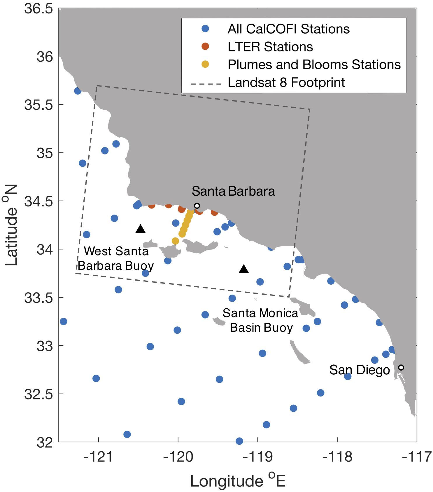
Figure 1. In situ data collection sites (orange, yellow, and blue markers) in the Southern California Bight used for temperature to nitrate relationships in the Santa Barbara Channel, California.

Temperature and nitrate data from all cruises were binned into two groups according to a seasonal, climatological pattern in the Southern California Bight: cool and wet winter months (December – May), and warm and dry summer months (June – November) (Otero and Siegel, 2004). Temperature and nitrate data were also binned by coastal vs. offshore (at least 10 km from the nearest coast), and sub-regionally, (northern: >34.15°N and < −120.5°E, central: from 33.75°N to 34.41°N and −120.4°E to −119.3°E, and southern: < 34.03°N and >−119.3°E) inside the Southern California Bight (Supplementary Figure S1). A GAM was fit for the two seasonal, three regional, and coastal/offshore temperature and nitrate datasets using the mgcv package in R with a Tweedie error structure (power function = 1.3; k = 10).

Satellite Imagery

Sea surface temperature (SST) imagery from multiple satellite sensors were used to produce seawater nitrate estimates with the empirical seasonal T2N relationships developed in this study. One kilometer resolution SST imagery was obtained via a combined MODIS/VIIRS-derived product for the Southern California Bight⁴; while 100 m resolution data from the Landsat 8 TIRS thermal band was used to derive high spatial resolution SST products in the Santa Barbara Channel⁵. An atmospheric correction was applied to the Landsat 8 imagery by scaling brightness values with fully processed 1 km SST product data (Snyder et al., 2017). Clouds, cloud shadows and land were masked from the Landsat 8 SST imagery using the Fmask algorithm (Zhu et al., 2015), and fog banks and airplane contrails were manually removed. Imagery was processed for twelve clear Landsat 8 overpass dates between 2016 and 2018, and then five of these images that displayed the best results from the atmospheric correction step (as well as the greatest dynamic range in nutrient values throughout the Channel), were chosen to represent the highest spatial resolution imagery available. Landsat 8-derived SST imagery were validated with SST data from four NOAA ocean observing buoys in the Santa Barbara Channel (buoys 46218 Harvest, 46054 West Santa Barbara, 46053 East Santa Barbara, and 46217 Anacapa Passage; r² = 0.93, mean error = 0.23°C, mean absolute error = 0.59°C, and linear fit equation y =  1.2x− 1.2). Buoy temperature time series from the Santa Monica Basin and West Santa Barbara (Figure 1) were also converted to time series of nitrate concentration using the T2N relationships developed in this study. These buoy time series were used to validate seawater nitrate estimates from the 1 km MODIS/VIIRS-derived product described above.

Spatial Scaling Analysis

We performed a scaling analysis to examine the effect of using SST products with different spatial resolutions to produce maps of seawater nitrate concentration. We started with a processed Landsat 8 100 m SST image and degraded the spatial resolution to produce 1, 2, 4, 9, 15, and 25 km pixel scale imagery of nitrate concentration via two methods (Figure 2).

FIGURE 2

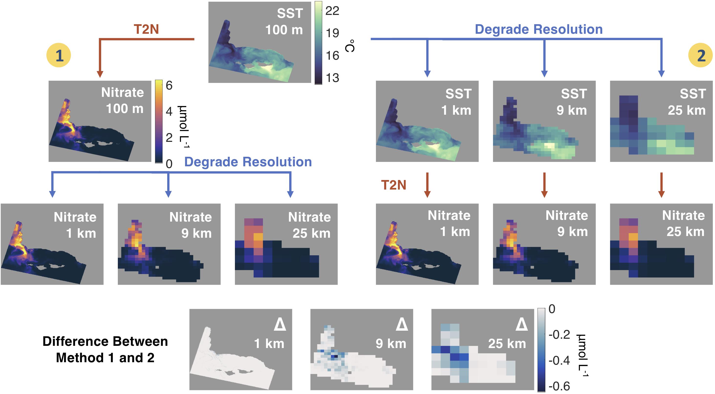
Figure 2. Description of the two methods of estimating nitrate from sea surface temperature (SST) imagery for the Santa Barbara Channel region using Landsat 8 thermal images from October 22, 2017. Method 1 preserves the magnitude of nitrate estimations at the native 100 m scale by first passing the SST data through the empirical temperature to nitrate (T2N) relationship, then degrading the spatial resolution. Method 2 approximates a data user selecting a SST product at a commonly available spatial resolution and then applying the T2N relationship. The bottom rows show the difference in estimated nitrate concentrations between Method 1 and 2 at each spatial resolution.

The first method preserves the high-resolution nitrate estimates by spatially degrading a 100 m nitrate product (assuming this product is “truth”), and the second method simulates the use of a lower resolution SST product by first spatially degrading the 100 m SST image before estimating the nitrate concentrations. We then found the difference in nitrate concentration between the two methods as the spatial resolution of the imagery was decreased. Differences in modeled seawater nitrate concentration were quantified using simple linear regressions. We also investigated the spatial error within a spatially degraded pixel by quantifying the fine scale physical processes hidden by using lower spatial resolution imagery. These fine scale (100 m) errors due to changing resolution were quantified by fitting normal probability distribution functions to the error distributions at each spatial scale.

Temporal Scaling Analysis

We performed a temporal scaling analysis to examine the effect of averaging SST through time on estimated seawater nitrate concentration. Temperature measurements were made every 10 min by the Santa Monica Basin buoy and West Santa Barbara buoy, and we sampled the timeseries (blue trace, Figure 3) at 1:30PM local time each day to mimic a satellite SST acquisition. These daily temperatures were then averaged over several time intervals (5, 10, 15, and 30 days) to simulate SST products at commonly available temporal resolutions (Figure 3).

FIGURE 3

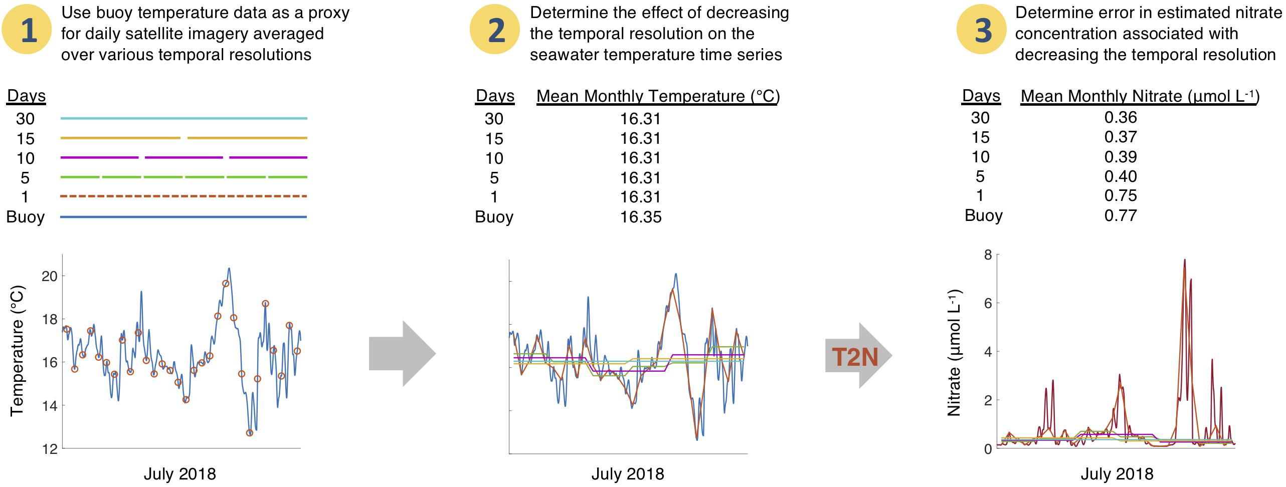
Figure 3. (1) Continuous temperature data (blue line) from a buoy was sampled daily to simulate daily satellite SST determinations (red dots). (2) These daily temperatures are then averaged over four temporal resolutions (5, 10, 15, and 30 days; shown as colored lines plotted over the continuous buoy data). The mean SST across the entire time series for each temporal resolution is shown. (3) Use empirical temperature to nitrate relationship (T2N) to estimate time series of nitrate concentration which are plotted over the continuous estimated nitrate concentration derived from the buoy temperature data (maroon line). The mean estimated nitrate concentration across the entire time series for each temporal resolution is shown.

These averaged temperature intervals were then converted to nitrate concentration and compared to the mean nitrate concentration estimated from the individual daily buoy temperatures over the same time period. The accuracy of the nitrate concentration estimate was determined using the mean absolute error for each temporal resolution (MAE_k), defined as:

$$MA{E}_k=\frac{1}{n}\sum _{i=1}^n|N_{k,i}^{Satellite}-N_{k,i}^{Buoy}|(1)$$

where $N_{\mathrm{k},\mathrm{i}}^{\text{Satellite}}$ is the estimated nitrate concentration from the simulated daily satellite SST averaged over each temporal resolution k, $N_{\mathrm{k},\mathrm{i}}^{\text{Buoy}}$ is the estimated nitrate concentration from the continuous buoy temperature measurements, and n is the total number of absolute error determinations. Mean absolute error is an unambiguous measure of error compared to root mean squared error because it is less sensitive to the distribution of error magnitudes (Willmott and Matsuura, 2005). To quantify bias in the estimation of nitrate concentration, we determined the mean error for each temporal resolution (ME_k) which was calculated as:

$$M{E}_k=\frac{1}{n}\sum _{i=1}^n\left(N_{k,i}^{Satellite}-N_{k,i}^{Buoy}\right)(2)$$

Cloud cover limits the ability of satellites to measure SST and varies seasonally. In order to account for the effect of variable cloud cover, a fraction of daily SST values (0.1, 0.2, 0.3, 0.4, 0.5, 0.6, 0.7, and 0.8) were randomly removed from each time interval before averaging was completed. Mean absolute error and mean error were then determined from these estimated nitrate concentrations as stated above.

Siting Analysis

We performed a siting analysis for all areas in the United States portion of the Southern CA Bight. Since the technology of farm design is changing rapidly, we included areas regardless of depth. We used daily, 1 km SST from the MODIS/VIIRS-derived product from 2002 to 2018 (see text footnote 4) and converted to nitrate concentration according to the seasonal T2N relationships derived in this study. We then calculated the mean and coefficient of variation of nitrate concentration in the surface water across all dates and the mean nitrate concentration for each season.

We also determined the proportion of time that giant kelp farms exist in nutrient conditions to support adequate growth rates. Giant kelp has internal nitrogen stores to support growth for roughly 2 to 3 weeks (Gerard, 1982a) and frond elongation rate maximizes at seawater nitrate concentrations of 1 μmol L^–1 (Zimmerman and Kremer, 1984). Therefore, we examined the number of consecutive days when surface nitrate concentrations fell below 1 μmol L^–1 after interpolating each 1 km pixel’s SST time series with a piecewise cubic spline to remove missing values (Matlab function interp1 – “pchip”). When there were >21 days in a row below the 1 μmol L^–1 nitrate concentration threshold, we counted those days as a period of giant kelp nutrient stress. We then found the fraction of days with kelp nutrient stress to determine the KSI for each season for the entire study area. Low frequency climate cycles, like the North Pacific Gyre Oscillation (NPGO), affects nitrate delivery to the Southern California Bight (Di Lorenzo et al., 2008; Parnell et al., 2010). Stronger winds drive increased upwelling during positive NPGO years, and greater concentrations of nutrients are delivered to the surface (Di Lorenzo et al., 2008). We also determined the difference in the KSI for each season when the NPGO was in a negative versus a positive mode.

Results

Temperature to Nitrate Relationship and Satellite Imagery

There were significant seasonal differences found in the T2N relationships developed from in situ temperature and nitrate data. The winter GAM had an R² = 0.83; p < 0.001; n = 2691; and the summer GAM had an R² = 0.91; p < 0.001; n = 2758, with winter months defined as December – May and summer months defined as June – November (Figure 4). The summer T2N relationship showed higher nitrate concentrations than the winter T2N relationship between 11 and 15°C. These seasonally specific relationships were used for all further analyses.

FIGURE 4

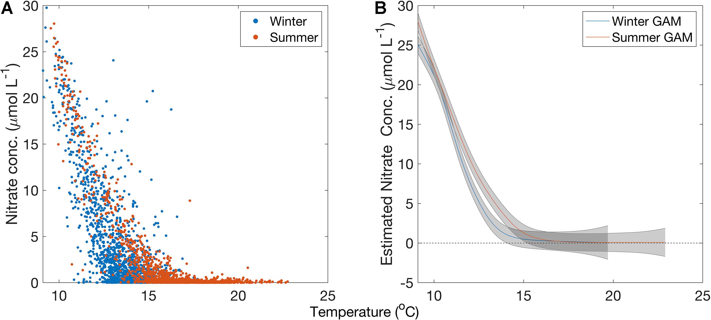
Figure 4. (A) Temperature and nitrate measurements separated by season in the Southern California Bight. Blue markers are datapoints collected during wintertime, red markers are datapoints collected during summertime. (B) Generalized additive model fit for temperature to nitrate relationships in the winter and summer months in the Santa Barbara Channel from 1980 to 2018 above 3 m depth. Blue line is the winter GAM, and red line is the summer GAM. Gray bars are the standard error about the curve.

There were no significant differences found between coastal and offshore T2N relationships, nor were significant differences found between the three sub-regional T2N relationships (Supplementary Figure S1). The results are qualitatively similar to prior work in the region (cf. Omand et al., 2012 or Jacox et al., 2015 for summaries of coastal and offshore T2N relationships derived from in situ observations).

High spatial resolution maps of SST and estimated nitrate concentration (Figure 5) were generated for the Santa Barbara Channel on five clear days between 2016 and 2018 (October 3, 2016, October 19, 2016, October 22, 2017, November 10, 2018, and December 28, 2018).

FIGURE 5

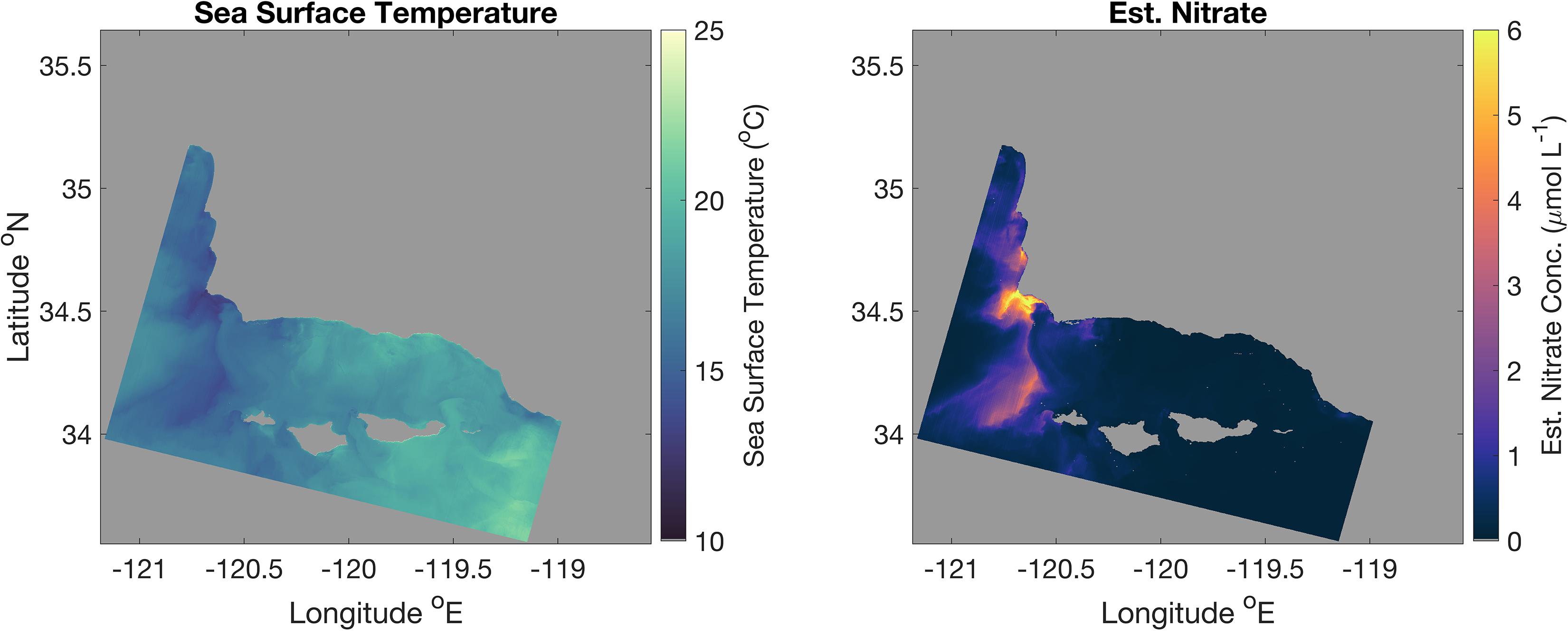
Figure 5. Landsat 8-derived SST and T2N estimated nitrate concentration imagery of the Santa Barbara Channel on October 19, 2016. Spatial resolution is 100 m.

Landsat 8-derived temperature data compared well to buoy validation data in the Santa Barbara Channel (r² = 0.93). Surface nitrate concentrations followed an inverse pattern to SST, as expected, where nitrate concentrations in the Santa Barbara Channel are typically highest in the western half of the channel, where cold, nutrient rich waters upwelled along the central coast of California are advected southward toward the western Channel Islands (Figure 5). This is observed in all five sets of Landsat imagery analyzed (Supplementary Figures S3–S6).

Satellite retrievals of SST (1 km MODIS/VIIRS product) and estimated nitrate concentration matched the general patterns of variability estimated from the continuous data at both buoys (Figure 6). General temperature patterns followed a seasonal cycle of highest values in the summer and lower values in the winter, while nitrate concentrations had an inverse pattern of peaks during the spring/winter and lows during the summer/fall.

FIGURE 6

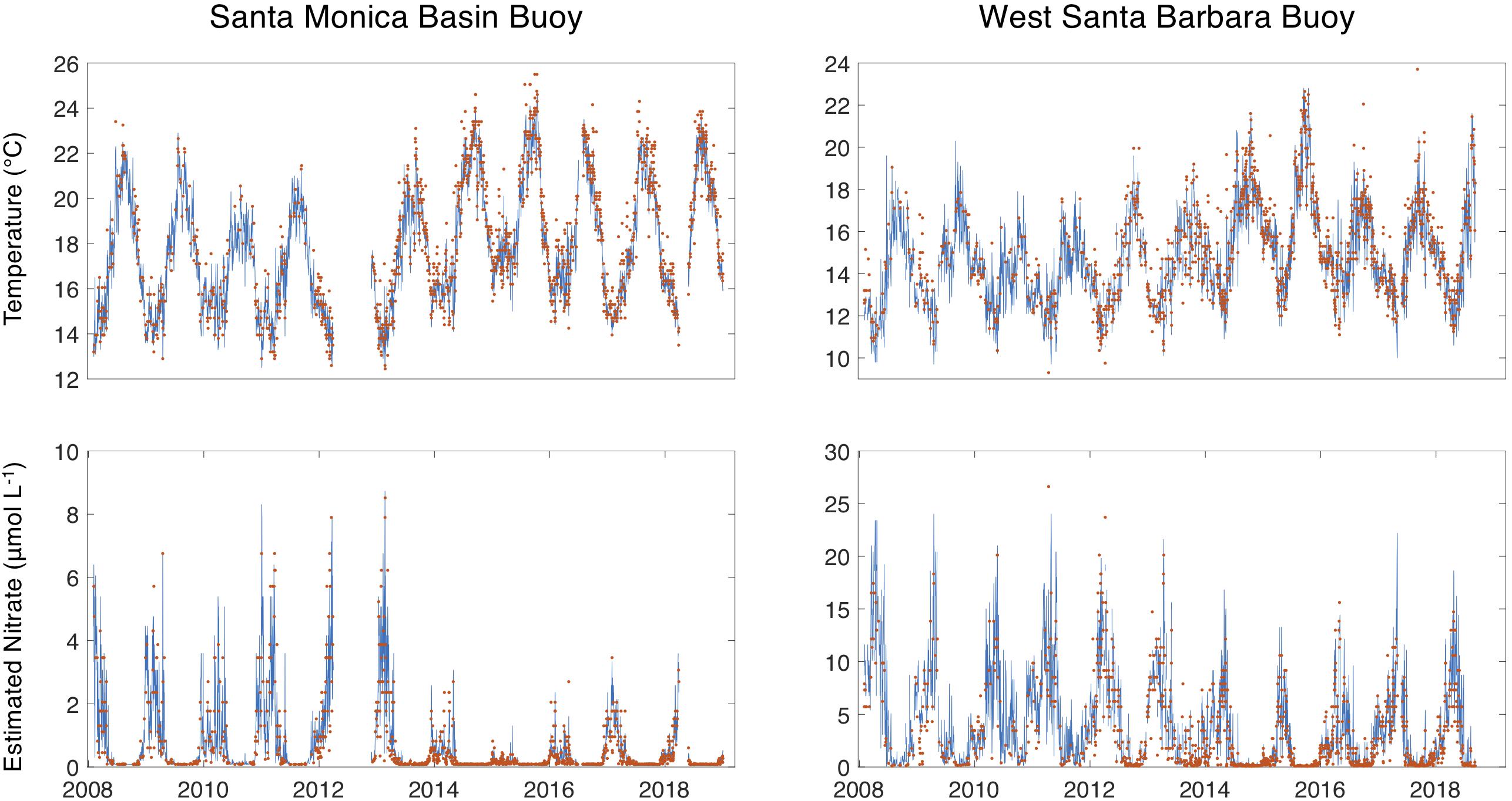
Figure 6. Continuous temperature and estimated nitrate concentrations time series from the Santa Monica Basin and West Santa Barbara buoys are shown as blue lines. The red dots show the daily SST and daily estimated nitrate concentrations from the 1 km, MODIS/VIIRS-derived SST product.

Comparisons of SST between the buoys (West Santa Barbara and Santa Monica Basin) and the satellite product were highly significant and more strongly correlated (r² = 0.93 and 0.95, p < 0.001) than the estimated seawater nitrate concentrations (r² = 0.89 and 0.79, p < 0.001) because nitrate estimates contain error from both satellite temperature estimates as well as the T2N relationship. Both mean absolute error and mean error were greater in magnitude for both SST and nitrate concentration for the West Santa Barbara buoy than the Santa Monica Basin buoy (Table 1).

TABLE 1

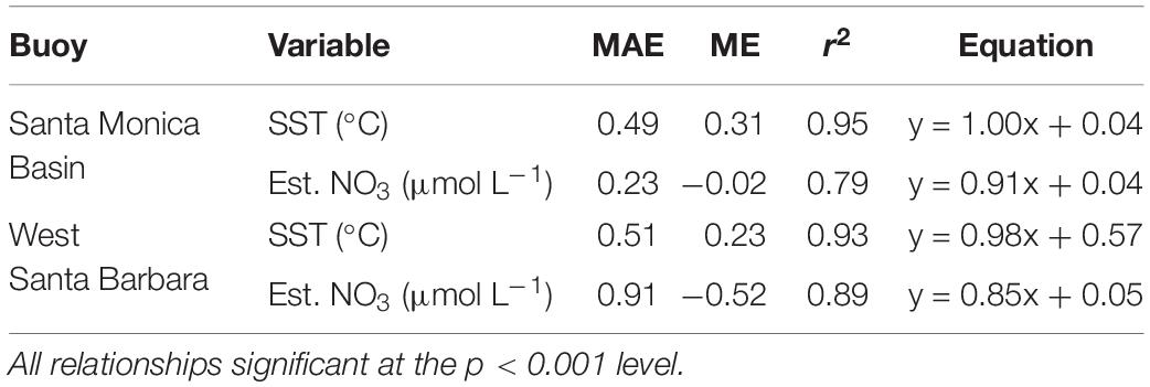
Table 1. The mean absolute error (MAE), mean error (ME), coefficient of determination (r²), and linear equation for relationships between sea surface temperature (SST) and estimated nitrate concentration (Est. NO₃) between buoys and satellite determinations (1 km) MODIS/VIIRS-derived SST product.

Spatial Scaling Analysis

The spatial scaling analysis showed that values of T2N estimated nitrate concentrations were reduced as the spatial resolution of the image was decreased (Figure 7). As the spatial resolution was degraded from 1 km to 25 km, nitrate concentrations greater than 1 μmol L^–1 were disproportionately underestimated and pixel nitrate concentration magnitude was reduced (Figure 7 and Supplementary Figures S3–S6).

FIGURE 7

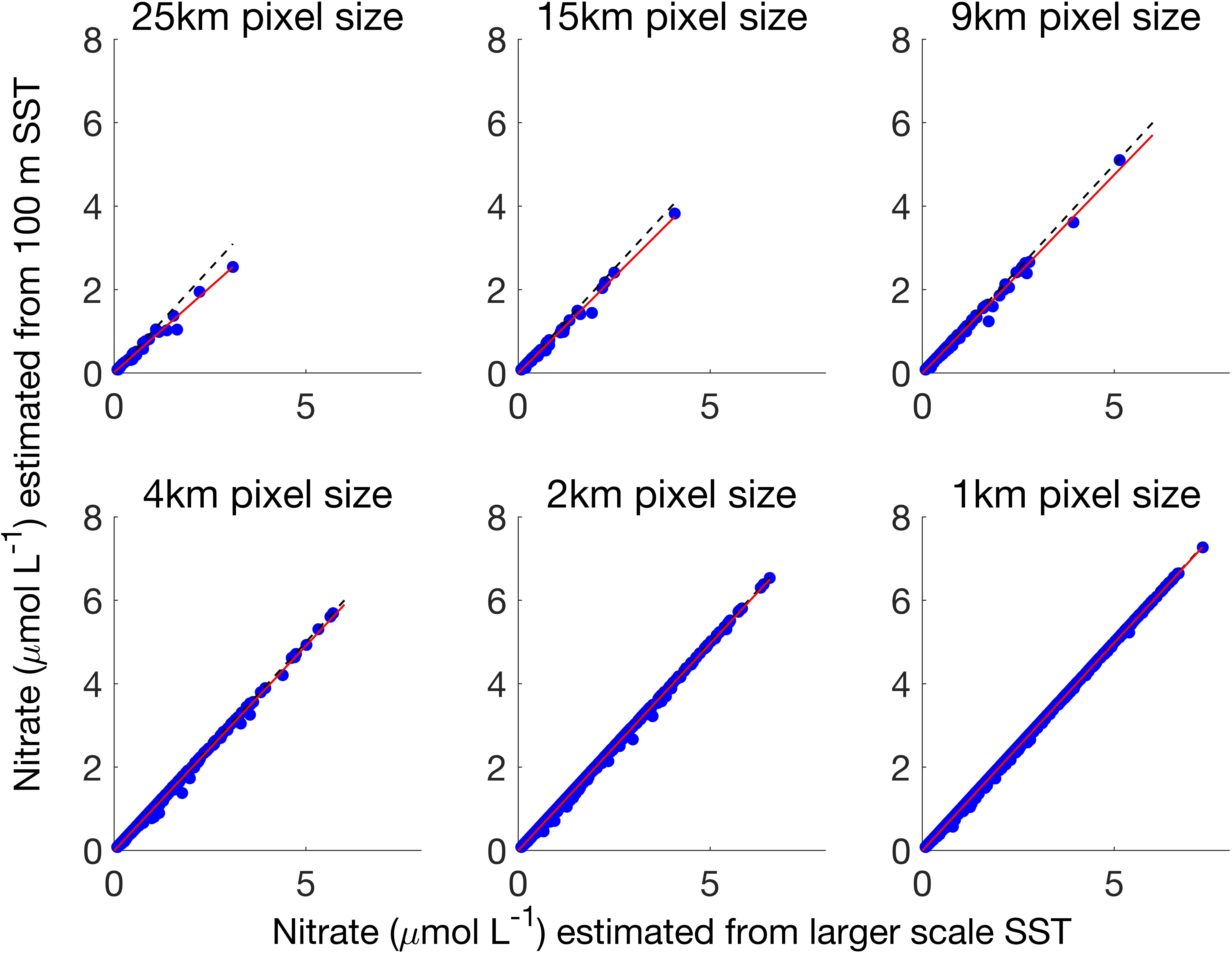
Figure 7. Nitrate concentrations for 25, 15, 9, 4, 2, and 1 km spatial resolution nitrate products calculated from the 100 m Landsat 8 SST product (x-axis) and the larger spatial resolution Landsat 8 SST product (y-axis). Red line is regression fit, dashed black line is 1:1. Image was collected on October 19, 2016.

As the spatial resolution was degraded, local scale variations in nitrate concentration were lost. As spatial resolution decreased from 1 km to 25 km, the standard deviation of the distribution of errors became larger, indicating that the level of error increased over a greater number of pixels (Figure 8). The mean of the error distribution decreased from zero to negative values as the spatial scale increased from 1 km to 25 km, indicating that local scale nitrate concentration was more often underestimated.

FIGURE 8

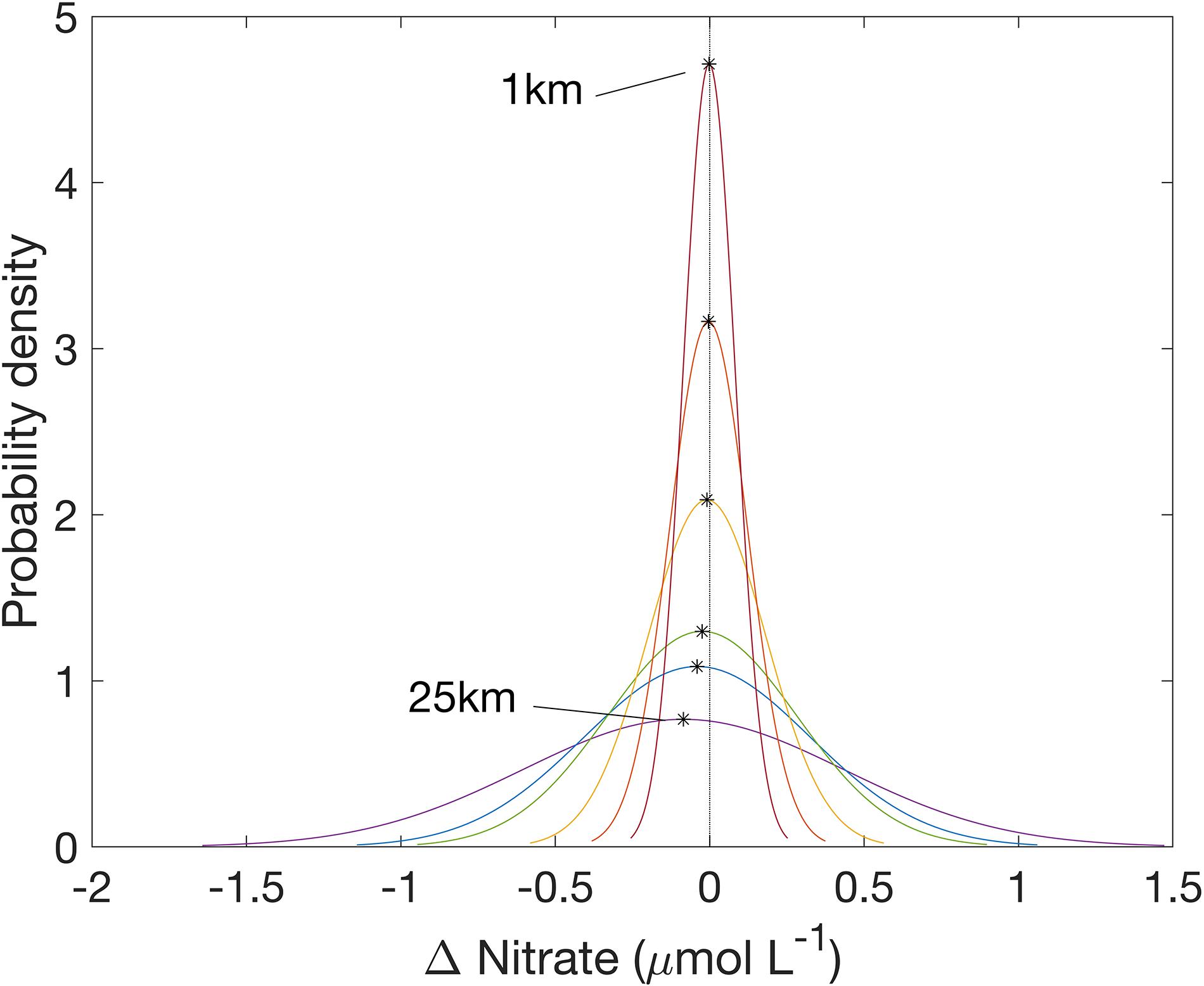
Figure 8. Normal curve fit of error distribution in nitrate product from October 19, 2016. Black stars are the mean error at each spatial resolution.

Maps of the difference in estimated nitrate concentration between the 100 m product and the 25 km product show the higher values of nitrate were diminished, (up to 5 μmol L^–1) in places where there was higher spatial variability in SST, such as around Point Conception in the northwest and around the Channel Islands (Figure 9).

FIGURE 9

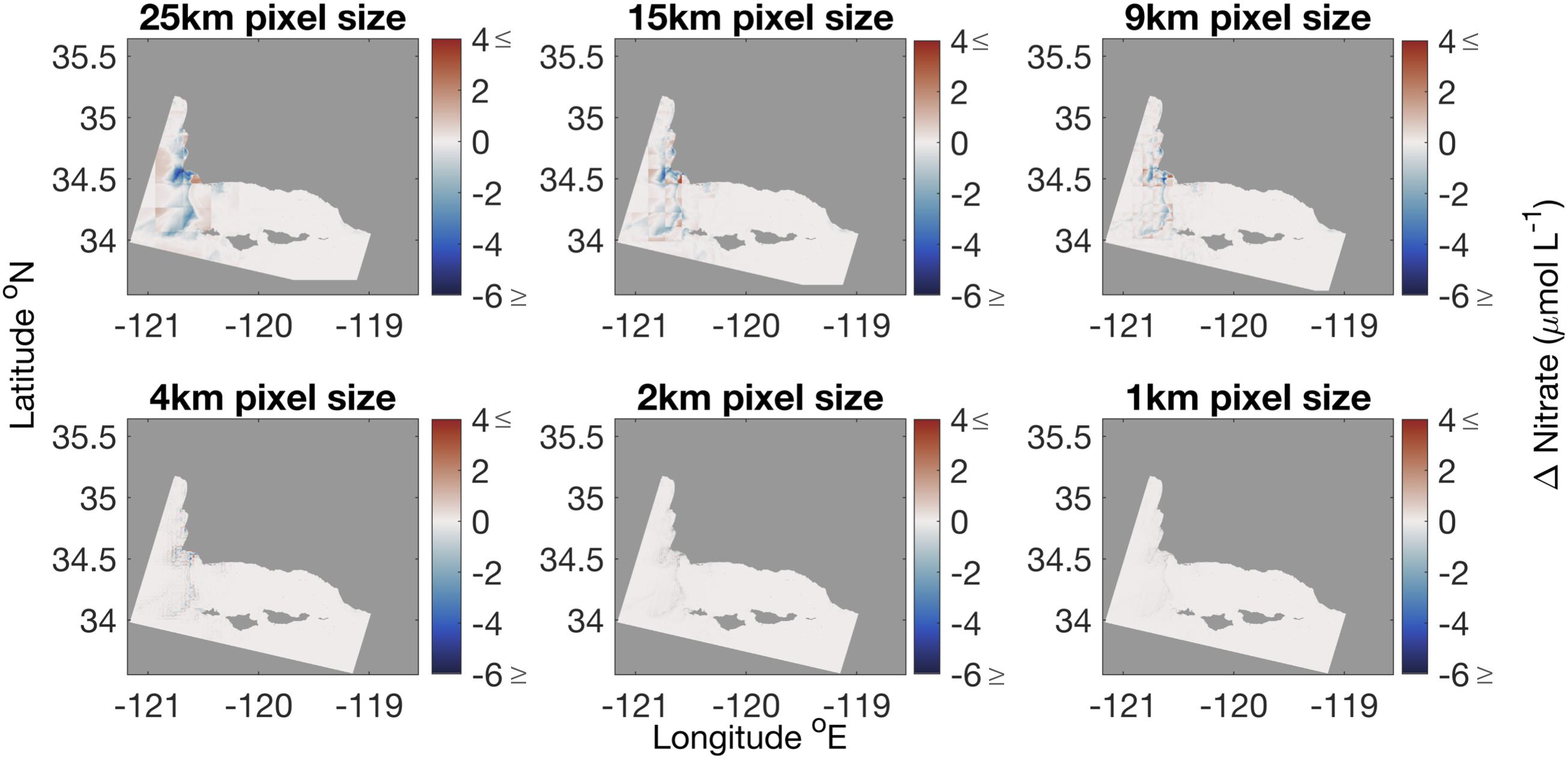
Figure 9. Difference between nitrate calculated from 100 m SST product and nitrate calculated from coarser spatial resolution SST products. Lower spatial resolution products diminished areas with high nitrate levels. Original Landsat 8 imagery was collected on October 19, 2016.

Temporal Analysis Results

The temporal scaling analysis showed that increasing the temporal averaging of daily SST imagery negatively biased nitrate concentration estimates (Figure 10). The average MAE (μmol L^–1) across all cloud contamination fractions did not show large changes as temporal scale increased for both buoys (West Santa Barbara, 0.66 to 0.64 and Santa Monica Basin, 0.13 to 0.14). However, there were large increases in MAE as the degree of cloud contamination increased, when averaged over all temporal scales (West Santa Barbara, 0.47 to 0.86 and Santa Monica Basin, 0.10 to 0.17), meaning that a reduction in the number of images due to cloud cover affected MAE more than averaging samples over a specific time period. The magnitude of the ME (μmol L^–1) increased and became more negative as the temporal scale increased (West Santa Barbara, −0.27 to −0.50 and Santa Monica Basin, −0.06 to −0.12) and displayed a smaller effect associated with increasing cloud contamination (West Santa Barbara, −0.42 to −0.32 and Santa Monica Basin, −0.09 to −0.07). Meaning that averaging samples over a specific time period led to a greater negative bias compared to a reduction in available imagery due to cloud cover.

FIGURE 10

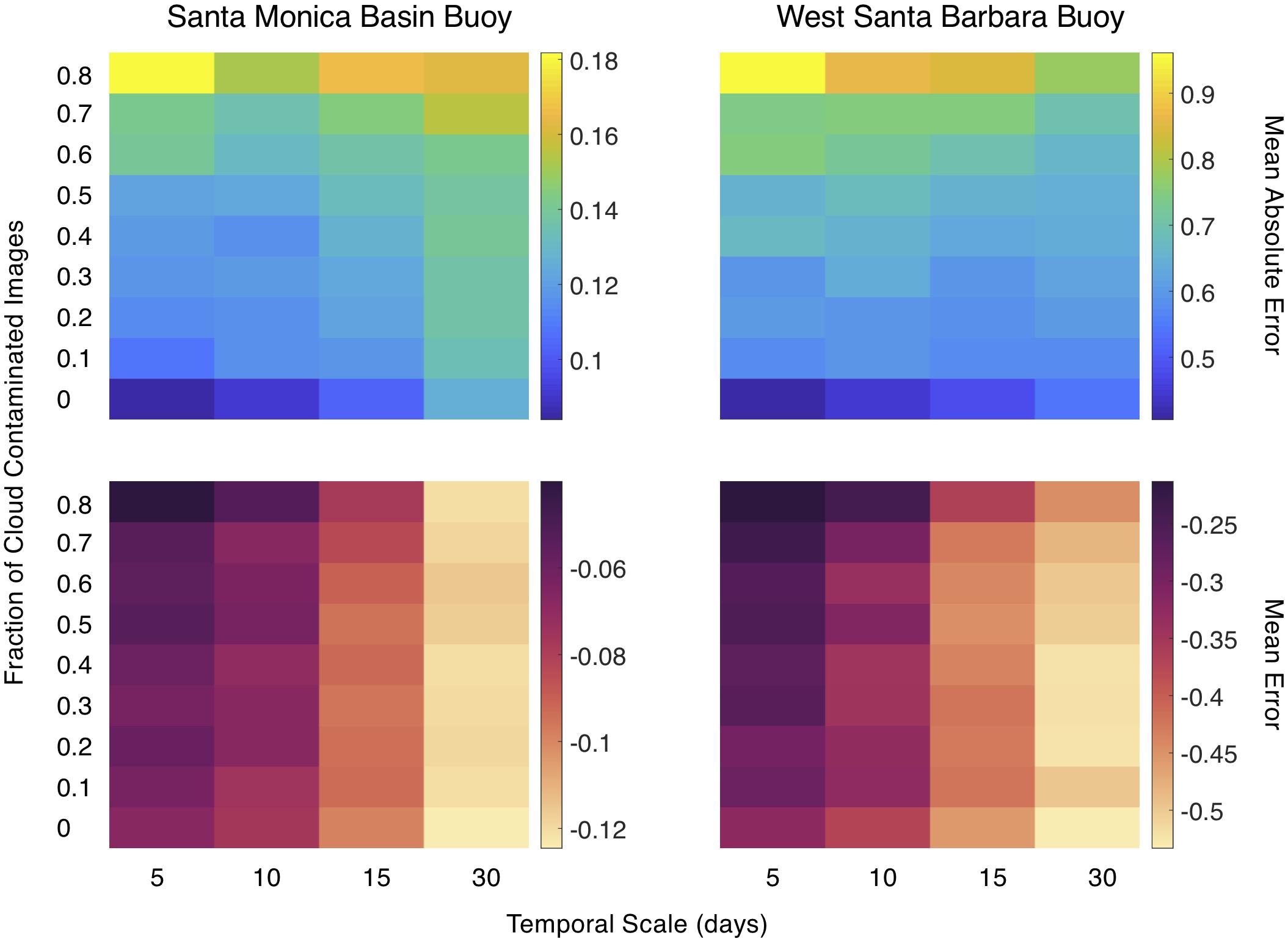
Figure 10. Mean absolute error and mean error in estimated nitrate concentration (μmol L^–1) as a function of the temporal resolution of the simulated SST imagery and the fraction of daily temperature images contaminated with cloud cover.

Siting Analysis

The siting analysis shows areas in the Southern California Bight that maintain consistent nitrate levels above 1 μmol L^–1 at the surface in all seasons, and some areas that exhibit seasonal and interannual differences. We found that nitrate concentrations remain elevated in areas north of Pt. Conception and in the western SB Channel throughout the time series, with a coefficient of variation of nitrate concentration close to 1 (Figure 11).

FIGURE 11

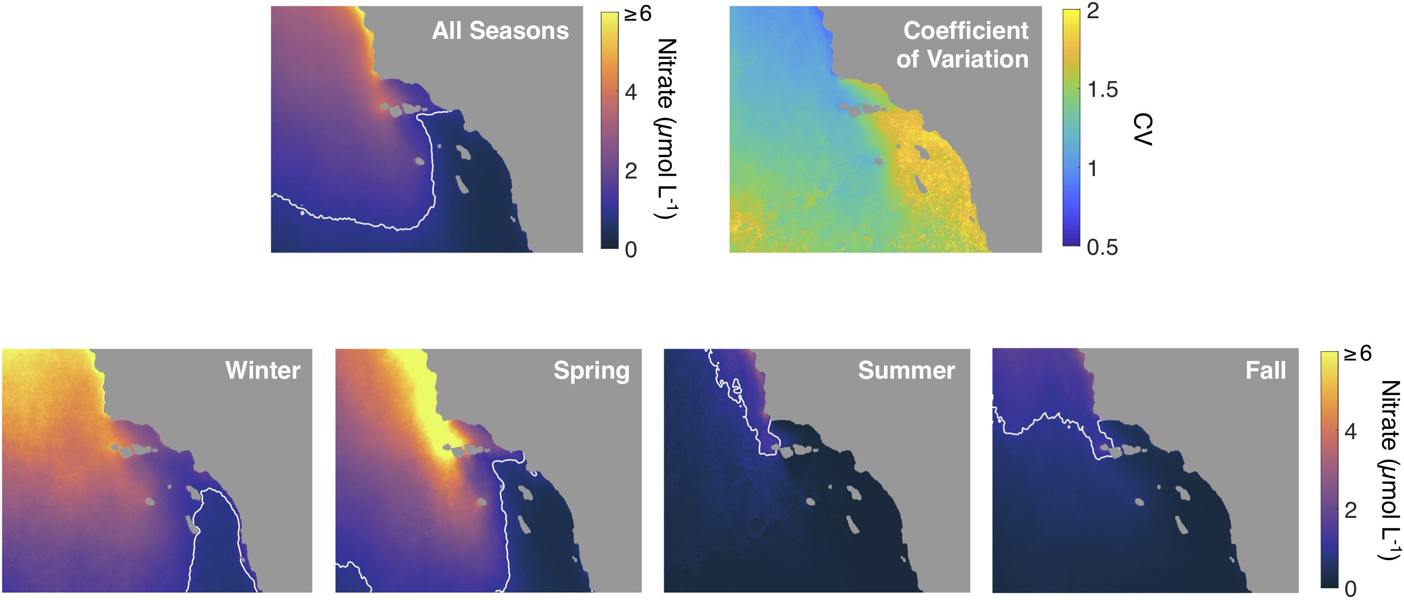
Figure 11. Top row: Mean and coefficient of variation (CV) of estimated nitrate concentration over the study area across all seasons. Bottom row: Mean estimated nitrate concentration across each season over the study area. White contour line shows the location of the 1 μmol L^–1 nitrate concentration front.

The coefficient of variation was higher in the rest of the SB Channel and close to 2 in much of the southeastern quadrant of our study area. Seasonal patterns of nitrate concentration were >1 μmol L^–1 for most of the study area in winter with increased concentrations in the northern half of the study area in spring. Summer and fall were characterized by reduced nitrate concentrations over the vast majority of the study area.

The KSI was low during the winter and spring seasons, the fraction of nutrient stress was close to zero throughout most of the Santa Barbara Channel and into the open ocean beyond the Channel Islands (Figure 12A). In the summer season KSI values were high, especially in the eastern half of the Channel and close to shore, where the fraction of nutrient stress was well above 0.8. There was moderate nutrient stress in the fall season, the stress fraction was above 0.5 in most of the SB Channel and southward.

FIGURE 12

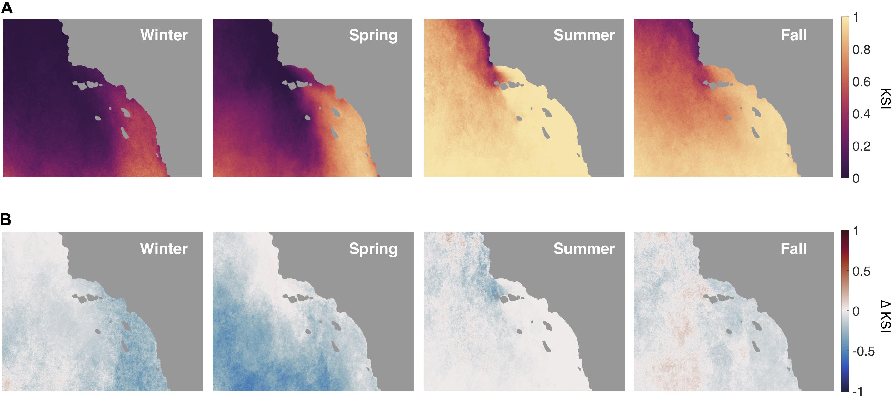
Figure 12. (A) The Kelp Stress Index (KSI) for each season over the study area. The KSI is the proportion of the season where kelp is nutrient stressed. Nutrient stress is defined as greater than 21 consecutive days of seawater nitrate concentration less than 1 μmol L^–1. (B) The difference in the KSI for each season when the North Pacific Gyre Oscillation (NPGO) is in a positive versus a negative mode.

During the positive phase of the NPGO the spatial pattern of nutrient stress changed the most during the spring season (Figure 12B). There was a decrease in KSI in areas offshore and south of the channel, in some places by as much as 0.5. The winter season also had a strong reduction in stress fraction, especially along the coast and to the southeast. The summer only had weak reductions in KSI near Point Conception, and the fall had mild reductions in the channel and along the southeast coast.

Discussion

Siting of Kelp Aquaculture Farms

Estimated surface nitrate concentration imagery show seasonal means that follow expectations for the Southern California Bight (Figure 11). Spring upwelling leads to elevated nitrate concentrations, especially in the northern and western halves of the study area. The SE quadrant of the study area can have less than 1 μmol L^–1 nitrate in surface waters for much of the year; and with CV’s of around 2, this area shows a great degree of variability through time. For kelp aquaculture, and especially farms fixed to the seafloor, areas with more stable nutrient conditions (both seasonally and interannually, i.e., the northern and western areas) should lead to more stable aquaculture production and should be considered in spatial planning analyses (Gentry et al., 2017; Lester et al., 2018). The Santa Barbara Channel is uniquely protected from exposure to wave action and high-resolution thermal imagery could be especially useful for identifying areas with nutrient concentrations high enough to support year-round kelp growth (Cabral et al., 2016).

The analysis of the KSI (i.e., fraction of days with kelp nutrient stress) shows that much of the study area is not under potential nitrate stress for the winter and spring seasons (Figure 12). During summer and fall the northern half of the study area can still display low kelp nutrient stress, but low nutrient surface waters dominate during summer in the SE quadrant and as they flow into the Santa Barbara Channel from the east and increase nutrient stress (Harms and Winant, 1994; Otero and Siegel, 2004). There are areas in the Southern California Bight that maintain less than ideal conditions for kelp growth (mean nitrate concentration stays below 1 μmol L^–1 nitrate as indicated by the white contour line in Figure 11). Nevertheless, there are kelp forests that occur for periods of several years in the SE quadrant of the map despite a high average KSI, for example, along the coast of San Diego, CA.

By incorporating decadal forcing like NPGO into the siting analysis we found valuable information that may have otherwise been missed by the averaged data through time. When the NPGO was positive, areas in the southern portion of the study area increased in their proportion of time with adequate nutrients for kelp growth, especially in the winter and spring. In fact, the NPGO is an important interannual driver of kelp canopy biomass dynamics along the California coast and natural kelp forests in these southern areas may only form canopies during positive NPGO years (Parnell et al., 2010; Cavanaugh et al., 2011; Bell et al., 2015a). It follows that engineered kelp farms planted in areas that typically experience low nitrate conditions may only be successful during high NPGO periods. We can learn from the dynamics of natural kelp systems in these low nitrate areas, especially if planned aquaculture requires that no external fertilizers are applied. The KSI is modulated by factors other than mean seasonal temperature and nutrient concentrations, so it is helpful to consider low frequency marine climate oscillations, like the NPGO, that may allow kelp to persist (Di Lorenzo et al., 2008). In the Santa Barbara Channel the KSI never exceeds 0.5, except in the Summer and Fall seasons near the eastern section and along the mainland coast. This highlights the western Santa Barbara Channel as an ideal site for maintaining kelp growth at the surface in offshore aquaculture during both negative and positive NPGO years.

It is important to note that this study only covers nitrate concentrations at the surface, and stratification and internal waves may be responsible for translocation of nutrients at depth (Zimmerman and Kremer, 1984; McPhee-Shaw et al., 2007). Despite this, we know that kelp canopy health declines when surface waters warm and nitrate decreases, both seasonally and during marine heatwaves, and thus surface waters are very important to monitor for kelp canopy condition and growth (Bell et al., 2018; Cavanaugh et al., 2019). While the spatial resolution of the MODIS 1 km product adequately captures surface patterns of SST and nitrate, it is important to note that the temporal resolution of satellite imagery only provides a snapshot of conditions at a single moment during the day. As such, this daily measurement likely misses oceanographic events, some of which could be especially important for supporting kelp growth. Internal waves are strong at 12 h periods and drive influxes of upwelled water into the Santa Barbara Channel, so for siting purposes it would be advantageous to collect continuous or hourly measurements with moored sensors that can capture these events and supplement satellite datasets (Zimmerman and Kremer, 1984).

These maps do not directly identify the best overall areas to site a kelp farm, but they do offer spatially and temporally explicit information to help with the decision-making process, as several factors will come into play depending on farm design, permitting, economic forces, and environmental impacts. As a foundation species and ecosystem engineer, giant kelp serves as a habitat for bryozoans, bacterial colonies, fishes etc, and floating kelp farms in the open ocean could have positive and/or negative effects on surrounding ecosystems by modulating local nutrient availability. Rather than solely rely on nitrate concentration, it is better to map how the organism of interest will respond to these nutrient dynamics. Maps of nutrient stress periods show areas where kelp production may suffer seasonally. Sainz et al. (2019) showed that bivalve aquaculture is also expected to do poorly in the Southern California Bight during these negative NPGO periods, however, Lester et al. (2018), showed that finfish aquaculture may benefit from warmer waters, conditions that would be common during this period. Due to the nature of decadal climate cycles in the Southern California Bight, it may be worthwhile to examine a dynamic approach to marine spatial planning, where kelp aquaculture could shift to other products during negative periods of the NPGO.

Effect of Spatial Scaling on Nitrate Estimates

Spatially degrading SST tends to underestimate the amount of nitrate in the surface waters due to the non-linearity of the T2N relationship. This is most apparent at the lowest spatial resolutions (25, 15, and 9 km in Figure 7) where the best fit line slope is lower than the 1:1 line. The largest effect is seen at nitrate values between 1 and 4 μmol L^–1 because this area is located at the curve of the T2N relationship, where the relationship is the most non-linear (Figure 4). At low nitrate values there is less of an effect because there is little nitrate in the water from 16°C to 24°C, thus averaging does not affect these lower values as much. Accurate nitrate concentration estimates around 1 – 4 μmol L^–1 are important because this is a critical concentration range for the growth of giant kelp (Gerard, 1982b; Bell et al., 2015a). Uptake rates by giant kelp vary non-linearly with ambient seawater nitrate concentration, and the nitrogen uptake rate changes the fastest over this 1 – 4 μmol L^–1 range (Gerard, 1982b). Thus, an error in estimating sea surface nitrate concentration, especially at low spatial resolutions, can lead to disproportionate errors in estimating nitrogen uptake by kelp. As errors tend to underestimate nitrate concentrations, larger spatial scale estimates may exclude areas as potential sites for kelp aquaculture.

Fine scale physical processes that bring cool, nutrient-rich water to specific sites can be hidden when the spatial resolution of remote sensing imagery is degraded. This is shown in the probability distribution functions (Figure 8) and maps of error (red and blue areas in Figure 9) at the 25, 15, and 9 km scale. Localized areas of upwelling, such as coastline and seamounts, or eddy formation (around the Channel Islands and headlands) may be good places for aquaculture but are often missed in lower spatial resolution imagery (Broitman and Kinlan, 2006; Bell et al., 2015b). The spatial scaling analysis showed that, under most circumstances, 1, 2, and 4 km resolution imagery compared well to the 100 m scale nitrate estimates for this study area.

Effect of Temporal Scaling on Nitrate Estimates

One-kilometer MODIS satellite retrievals performed well for SST and nitrate dynamics as seen in validation data by continuous buoy measurements in both cool and warm areas of the Southern California Bight (Table 1). The increased magnitude of MAE and ME of estimated nitrate concentrations in the West Santa Barbara buoy were likely caused by the higher magnitudes of nitrate at that site relative to the Santa Monica Basin site. As part of the temporal scaling analysis, higher values in MAE were due to the higher fraction of cloud contaminated daily SST estimates as opposed to the increase in temporal scale (Figure 10). Offshore areas to the west of the Channel Islands and Pt. Conception are generally cloudier than areas inside the Channel Islands (Supplementary Figures S2A,B), and overcast and cloudy conditions often persist throughout the summer and fall seasons over the Santa Barbara Channel. This makes it difficult to build an accurate climatology, as clear imagery are sometimes only available once or twice per week. We see that as new satellites come online, such as VIIRS in 2012, the increased number of passes allows at least one sensor to get a clear image of daily SST more often. The future launch of Landsat 9, scheduled for 2020, promises an improved TIRS-2 sensor that will reduce stray light issues in Landsat 8’s thermal imagery, as well as increase global coverage and data collection. Improvements in future satellite missions, the addition of geostationary satellites, and greater cooperation between global space agencies will continue to mitigate this limitation (Castelao et al., 2006). For areas with persistent cloud cover and frequent storms (and thus lower SST and possibly higher nitrate concentrations) in situ monitoring will be necessary for farmers and stakeholders to observe local conditions.

On the contrary, increases in the ME are driven mostly by increases in temporal averaging and not cloud contamination. It is important to note that ME is always negative and becomes more negative as temporal scale (the averaging of daily SST determinations) increases. We cannot control the level of cloud contamination, but we can control the temporal scale at which we convert SST to nitrate concentrations. We would recommend that each daily determination of SST is converted to nitrate before averaging over time (Figure 2).

Conclusion

It is important to understand the implications of spatial and temporal scale of temperature data when estimating seawater nutrient fields for assessing the suitability of kelp aquaculture sites. We found that daily, 1 km SST imagery does an adequate job of replicating continuous buoy measurements. For studies in the NE Pacific, a merged daily 1 km multi-satellite product, like the one used in this study, captures a great deal of the variability in temperature and nitrate concentration in this system at a fine spatial and temporal scale. It is also important to remember that SST does not estimate temperature dynamics below the surface of the water, and that waters can be stratified in the summer. This stratification may hide subsurface dynamics of seawater nutrients. Future offshore aquaculture farms may use technology to overcome this, like farms which can alter buoyancy to sink below a nutricline or employ the use of artificial upwelling devices.

Data Availability Statement

Publicly available datasets were used in this study. These data can be found here: http://spg-satdata.ucsd.edu/, http://sbc.lternet.edu/, http://www.oceancolor.ucsb.edu/plumes_and_blooms/, and https://calcofi.org/.

Author Contributions

JS and TB developed the research concept and led the image and data analyses. JS and TB led the writing with contributions from DS, NN, and KC.

Funding

Funding was provided by the U.S. Department of Energy ARPA-E grant #DE-AR0000922, the NASA Plumes and Blooms grant #80NSSC18K0735 and MBON grant #NNX14AR62A, and the U.S. National Science Foundation grant for the SBC LTER – OCE #1831937.

Conflict of Interest

The authors declare that the research was conducted in the absence of any commercial or financial relationships that could be construed as a potential conflict of interest.

Acknowledgments

We would like to acknowledge the USGS for providing open source Landsat 8 imagery and Mati Kahru for providing the timeseries of processed SST imagery. We thank Nathalie Guillocheau and Stuart Halewood for data products from the Plumes and Blooms cruises, as well as the Santa Barbara LTER survey team and CALCOFI survey teams for their data collections and provisions.

Supplementary Material

The Supplementary Material for this article can be found online at: https://www.frontiersin.org/articles/10.3389/fmars.2020.00022/full#supplementary-material

Footnotes

1. ^ CalCOFI.org
2. ^ http://sbc.lternet.edu/
3. ^ http://www.oceancolor.ucsb.edu/plumes_and_blooms/
4. ^ http://spg-satdata.ucsd.edu/
5. ^ earthexplorer.usgs.gov

References

Bell, T. W., Cavanaugh, K. C., Reed, D. C., and Siegel, D. A. (2015a). Geographical variability in the controls of giant kelp biomass dynamics. J. Biogeogr. 42, 2010–2021. doi: 10.1111/jbi.12550

CrossRef Full Text | Google Scholar

Bell, T. W., Cavanaugh, K. C., and Siegel, D. A. (2015b). Remote monitoring of giant kelp biomass and physiological condition: an evaluation of the potential for the Hyperspectral Infrared Imager (HyspIRI) mission. Remote Sens. Environ. 167, 218–228. doi: 10.1016/j.rse.2015.05.003

CrossRef Full Text | Google Scholar

Bell, T. W., Reed, D. C., Nelson, N. B., and Siegel, D. A. (2018). Regional patterns of physiological condition determine giant kelp net primary production dynamics. Limnol. Oceanogr. 63, 472–483. doi: 10.1002/lno.10753

CrossRef Full Text | Google Scholar

Broitman, B. R., and Kinlan, B. P. (2006). Spatial scales of benthic and pelagic producer biomass in a coastal upwelling ecosystem. Mar. Ecol. Progre. Ser. 327, 15–25. doi: 10.3354/meps327015

CrossRef Full Text | Google Scholar

Brzezinski, M., Reed, D., and Harrer, S. (2013). Multiple sources and forms of nitrogen sustain year-round kelp growth on the inner continental shelf of the Santa Barbara Channel. Oceanography 26, 114–123. doi: 10.5670/oceanog.2013.53

CrossRef Full Text | Google Scholar

Burkepile, D. E., Allgeier, J. E., Shantz, A. A., Pritchard, C. E., Lemoine, N. P., Bhatti, L. H., et al. (2013). Nutrient supply from fishes facilitates macroalgae and suppresses corals in a Caribbean coral reef ecosystem. Sci. Rep. 3:1493. doi: 10.1038/srep01493

PubMed Abstract | CrossRef Full Text | Google Scholar

Cabral, R. B., Gaines, S. D., Johnson, B. A., Bell, T. W., and White, C. (2016). Drivers of redistribution of fishing and non- fishing effort after the implementation of a marine protected area network. Ecol. Appl. 27, 416–428. doi: 10.1002/eap.1446

PubMed Abstract | CrossRef Full Text | Google Scholar

Castelao, R. M., Mavor, T. P., Barth, J. A., and Breaker, L. C. (2006). Sea surface temperature fronts in the California current system from geostationary satellite observations. J. Geophys. Re.: Oceans 111, 1–13. doi: 10.1029/2006JC003541

CrossRef Full Text | Google Scholar

Cavanaugh, K. C., Reed, D. C., Bell, T. W., Castorani, M. C. N., and Beas-Luna, R. (2019). Spatial variability in the resistance and resilience of giant kelp in Southern and Baja California to a Multiyear Heatwave. Fron. Mar. Sci. 6:413. doi: 10.3389/fmars.2019.00413

CrossRef Full Text | Google Scholar

Cavanaugh, K. C., Siegel, D. A., Reed, D. C., and Dennison, P. E. (2011). Environmental controls of giant-kelp biomass in the santa barbara channel. California. Mar. Ecol. Progr. Ser. 429, 1–17. doi: 10.3354/meps09141

CrossRef Full Text | Google Scholar

Colombo-Pallotta, M. F., García-Mendoza, E., and Ladah, L. B. (2006). Photosynthetic performance, light absorption, and pigment composition of Macrocystis pyrifera (Laminariales. Phaeophyceae) blades from different depths. J. Phycol. 42, 1225–1234. doi: 10.1111/j.1529-8817.2006.00287

CrossRef Full Text | Google Scholar

Deysher, L. E., and Dean, T. A. (1986). In situ recruitment of sporophytes of the giant kelp, Macrocystis pyrifera (L.) C.A. Agardh: effects of physical factors. J. Exp. Mar. Biol. Ecol. 103, 41–63. doi: 10.1016/0022-0981(86)90131-0

CrossRef Full Text | Google Scholar

Di Lorenzo, E., Schneider, N., Cobb, K. M., Franks, P. J. S., Chhak, K., Miller, A. J., et al. (2008). North pacific gyre oscillation links ocean climate and ecosystem change. Geophysi. Res. Lett. 35, 2–7. doi: 10.1029/2007GL032838

PubMed Abstract | CrossRef Full Text | Google Scholar

Dugdale, R. C., Davis, C. O., and Wilkerson, F. P. (1997). Assessment of new production at the upwelling center at point conception, California, using nitrate estimated from remotely sensed sea surface temperature. J. Geophys. Res. 102, 8573–8585. doi: 10.1029/96jc02136

CrossRef Full Text | Google Scholar

Edwards, M. S., and Estes, J. A. (2006). Catastrophe, recovery and range limitation in NE Pacific kelp forests: a large-scale perspective. Mar. Ecol. Progr. Seri. 320, 79–87. doi: 10.3354/meps320079

CrossRef Full Text | Google Scholar

Eppley, R. W., Renger, E. H., and Harrison, W. G. (1979). Nitrate and phytoplankton production in southern California coastal waters. Limnol Oceanogr. 24, 483–494. doi: 10.4319/lo.1979.24.3.0483

CrossRef Full Text | Google Scholar

Fram, J. P., Stewart, H. L., Brzezinski, M. A., Gaylord, B., Reed, D. C., Williams, S. L., et al. (2008). Physical pathways and utilization of nitrate supply to the giant kelp, Macrocystis pyrifera. Limnol. Oceanogr. 53, 1589–1603. doi: 10.4319/lo.2008.53.4.1589

CrossRef Full Text | Google Scholar

Gentry, R. R., Lester, S. E., Kappel, C. V., White, C., Bell, T. W., Stevens, J., et al. (2017). Offshore aquaculture: spatial planning principles for sustainable development. Ecol. Evol. 7, 733–743. doi: 10.1002/ece3.2637

PubMed Abstract | CrossRef Full Text | Google Scholar

Gerard, V. A. (1982a). Macrocystis pyrifera in a Low-Nitrogen Environment. Mar. Biol. 66, 27–35. doi: 10.1007/BF00397251

CrossRef Full Text | Google Scholar

Gerard, V. A. (1982b). In situ rates of nitrate uptake by giant kelp, Macrocystis pyrifera (L.) C. Agardh: tissue differences, environmental effects, and predictions of nitrogen-limited growth. J. Exp. Mar. Biol. Ecol. 62, 211–224. doi: 10.1007/s00442-016-3641-2

PubMed Abstract | CrossRef Full Text | Google Scholar

Graham, M. H., Vasquez, J. A., and Buschmann, A. H. (2007). Global ecology of the giant kelp Macrocystis: from ecotypes to ecosystems. Oceanogr. Mar. Biol. 45, 39–88. doi: 10.1201/9781420050943.ch2

CrossRef Full Text | Google Scholar

Harms, S., and Winant, C. D. (1994). Synthetic subsurface pressure derived from bottom pressure and tide gauge observations. J. Atmos. Oceanic Technol. 11, 1625–1637. doi: 10.1175/1520-0426(1994)011<1625:sspdfb>2.0.co;2

CrossRef Full Text | Google Scholar

Henderikx-Freitas, F., Siegel, D. A., Maritorena, S., and Fields, E. (2016). Satellite assessment of particulate matter and phytoplankton variations in the Santa Barbara Channel and its surrounding waters: role of surface waves. J. Geophys. Res.: Oceans 122, 355–371. doi: 10.1002/2016JC012152

CrossRef Full Text | Google Scholar

Jacox, M. G., Bograd, S. J., Hazen, E. L., and Fiechter, J. (2015). Sensitivity of the California current nutrient supply to wind, heat, and remote ocean forcing. Geophys. Res. Lett. 42, 5950–5957. doi: 10.1002/2015gl065147

CrossRef Full Text | Google Scholar

Kamykowski, D., and Zentara, S. (1986). Predicting plant nutrient concentrations from temperature and sigma-t in the upper kilometer of the world ocean. Deep Sea Res. 33, 89–105. doi: 10.1016/0198-0149(86)90109-3

CrossRef Full Text | Google Scholar

Kamykowski, D., Zentara, S., Morrison, J. M., and Switzer, A. C. (2002). Dynamic global patterns of nitrate, phosphate, silicate, and iron availability and phytoplankton community composition from remote sensing data. Global Biogeoch. Cycles 16:25-1-25-29. doi: 10.1029/2001GB001640

CrossRef Full Text | Google Scholar

Kim, H. J., and Miller, A. J. (2007). Did the thermocline deepen in the California Current after the 1976/77 climate regime shift? J. Phys. Oceanogr. 37, 1733–1739. doi: 10.1175/jpo3058.1

CrossRef Full Text | Google Scholar

Konotchick, T., Parnell, P. E., Dayton, P. K., and Leichter, J. J. (2012). Vertical distribution of Macrocystis pyrifera nutrient exposure in southern California. Estuar.Coast. Shelf Sci. 106, 85–92. doi: 10.1016/j.ecss.2012.04.026

CrossRef Full Text | Google Scholar

Lester, S. E., Stevens, J. M., Gentry, R. R., Kappel, C. V., Bell, T. W., Costello, C. J., et al. (2018). Marine spatial planning makes room for offshore aquaculture in crowded coastal waters. Nat. Commun. 9, 945. doi: 10.1038/s41467-018-03249-1

PubMed Abstract | CrossRef Full Text | Google Scholar

McPhee-Shaw, E. E., Siegel, D. A., Washburn, L., Brzezinski, M. A., Jones, J. L., Leydecker, A., et al. (2007). Mechanisms for nutrient delivery to the inner shelf: observations from the santa barbara channel. Limnol. Oceanogr. 52, 1748–1766. doi: 10.4319/lo.2007.52.5.1748

CrossRef Full Text | Google Scholar

Morin, P., Wafar, M. V. M., and Corre, P. (1993). Estimations of nitrate flux in a tidal front from satellite-derived temperature data. J. Geophys. Res. 98, 4689–4695. doi: 10.1029/92jc02445

CrossRef Full Text | Google Scholar

Omand, M. M., Feddersen, F., Guza, R., and Franks, P. J. (2012). Episodic vertical nutrient fluxes and nearshore phytoplankton blooms in Southern California. Limnol. Oceanogr. 57, 1673–1688. doi: 10.4319/lo.2012.57.6.1673

CrossRef Full Text | Google Scholar

Otero, M. P., and Siegel, D. A. (2004). Spatial and temporal characteristics of sediment plumes and phytoplankton blooms in the Santa Barbara Channel. Deep Sea Res. 51, 1129–1149. doi: 10.1016/j.dsr2.2004.04.004

CrossRef Full Text | Google Scholar

Parnell, P. E., Miller, E. F., Lennert-Cody, C. E., Dayton, P. K., Carter, M. L., and Stebbins, T. D. (2010). The response of giant kelp (Macrocystis pyrifera) in southern California to low-frequency climate forcing. Limnol. Oceanogr. 55, 2686–2702. doi: 10.4319/lo.2010.55.6.2686

CrossRef Full Text | Google Scholar

Paulson, G. O. (1972). A study of Nutrient Variations in the Surface and Mixed Layer of Monterey Bay Using Automated Analysis Techniques. M.S. thesis, Nav. Postgraduate School, Monterey, CA.

Google Scholar

Peters, J. R., Reed, D. C., and Burkepile, D. E. (2019). Climate and fishing drive regime shifts in consumer-mediated nutrient cycling in kelp forests. Glob. Chang. Biol. 25, 3179–3192. doi: 10.1111/gcb.14706

PubMed Abstract | CrossRef Full Text | Google Scholar

Rodriguez, G. E., Reed, D. C., and Holbrook, S. J. (2016). Blade life span, structural investment, and nutrient allocation in giant kelp. Oecologia 182, 397–404. doi: 10.1007/s00442-016-3674-6

PubMed Abstract | CrossRef Full Text | Google Scholar

Sainz, J. F., Di Lorenzo, E., Bell, T. W., Gaines, S., Lenihan, H., and Miller, R. J. (2019). Spatial planning of marine aquaculture under climate decadal variability: a case study for mussel farms in southern California. Front. Mar. Sci. 6:253. doi: 10.3389/fmars.2019.00253

CrossRef Full Text | Google Scholar

Sathyendranath, S., Platt, T., Horne, E. P. W., Harrison, W. G., Ulloa, O., Outerbridge, R., et al. (1991). Estimation of new production in the ocean by compound remote sensing. Nature 353, 129–133. doi: 10.1038/353129a0

CrossRef Full Text | Google Scholar

Smith, J. M., Brzezinski, M. A., Melack, J. M., Miller, R. J., and Reed, D. C. (2018). Urea as a source of nitrogen to giant kelp (Macrocystis pyrifera). Limnol. Oceanogr. Lett. 3, 365–373. doi: 10.1002/lol2.10088

CrossRef Full Text | Google Scholar

Snyder, J., Boss, E., Weatherbee, R., Thomas, A. C., Brady, D., and Newell, C. (2017). Oyster aquaculture site selection using landsat 8-Derived sea surface temperature, turbidity, and chlorophyll a. Front. Mar. Sci. 4:190. doi: 10.3389/fmars.2017.00190

CrossRef Full Text | Google Scholar

Son, S., Platt, T., Bouman, H., and Lee, D. (2006). Satellite observation of chlorophyll and nutrients increase induced by Typhoon Megi in the Japan/East Sea. Geophys. Res. Lett. 33, 4–7. doi: 10.1029/2005GL025065

CrossRef Full Text | Google Scholar

Stewart, H. L., Fram, J. P., Reed, D. C., Williams, S. L., Brzezinski, M. A., Maclntyreb, S., et al. (2009). Differences in growth, morphology and tissue carbon and nitrogen of Macrocystis pyrifera within and at the outer edge of a giant kelp forest in California. USA. Mar. Ecol. Progr. Ser. 375, 101–112. doi: 10.3354/meps07752

CrossRef Full Text | Google Scholar

Willmott, C. J., and Matsuura, K. (2005). Advantages of the mean absolute error (MAE) over the root mean square error (RMSE) in assessing average model performance. Clim. Res. 30, 79–82. doi: 10.3354/cr00799

CrossRef Full Text | Google Scholar

Wood, S. N. (2006). Generalized Additive Models: An Introduction With R. London: Chapman and Hall/CRC.

Google Scholar

Zhu, Z., Wang, S., and Woodcock, C. E. (2015). Remote Sensing of Environment Improvement and expansion of the Fmask algorithm: cloud, cloud shadow, and snow detection for Landsats 4 – 7, 8, and Sentinel 2 images. Remote Sens. Environ. 159, 269–277. doi: 10.1016/j.rse.2014.12.014

CrossRef Full Text | Google Scholar

Zimmerman, R. C., and Kremer, J. N. (1984). Episodic nutrient supply to a kelp forest ecosystem in Southern California. J. Mar. Res. 42, 591–604. doi: 10.1357/002224084788506031

CrossRef Full Text | Google Scholar