Shoreline Variability at a Reef-Fringed Pocket Beach

Introduction

Pocket beaches, in which a stretch of sandy shoreline is bounded by headlands or other features that impede alongshore sediment transport, occur globally across a wide range of wave exposure regimes. Due to how these beaches are bound by barriers to sediment transport, they are often considered to be largely closed systems. Pocket beaches can be dominated by both cross-shore transport processes, that are primarily controlled by the incident wave energy (Harley et al., 2011; Blossier et al., 2017a), or alongshore transport that may cause beach rotation (Dehouck et al., 2009; Daly et al., 2014). In addition to limiting or preventing broad-scale alongshore transport, headlands or other bounding structures can introduce alongshore wave energy gradients (e.g., by shadowing obliquely incident waves), and act as wave reflectors particularly in the case of low frequency (infragravity waves) which can result in standing edge waves (e.g., Özkan-Haller et al., 2001; Masselink et al., 2004) along the pocket beach. Most research has focused on pocket beaches that are located along open coastlines (e.g., Vousdoukas et al., 2009; Horta et al., 2018). However, pocket beaches are also commonly fringed by coral or rocky reefs that create a semi-protected lagoon, which may have a significant influence on the beach morphodynamics processes.

For reef-fronted beaches, the general physical mechanisms that drive the hydrodynamic processes can be similar to those in other coastal environments in which wave breaking results in wave-driven currents (Monismith et al., 2013). These wave-driven currents are generated by radiation stress gradients dominated by wave breaking, resulting in wave setup gradients across the reef that can drive onshore mass fluxes over the reef if a lagoon is present (e.g., Gourlay and Colleter, 2005; Taebi et al., 2011; Lowe and Falter, 2015). While these same processes occur in open coast sandy beaches, reef environments also have additional complexity associated with steep slopes and high bottom roughness that can modify the nearshore hydrodynamics.

Along reef-fringed beaches, the importance of low-frequency infragravity (IG) waves with periods between 25 and 600 s has been highlighted in a number of studies (e.g., Hardy and Young, 1996; Péquignet et al., 2009; Pomeroy et al., 2012; Buckley et al., 2018). This is mostly a result of the dissipation of groups of sea-swell (periods < 25 s) waves by the shallow reef that leads to the generation of IG waves through both a breakpoint forcing mechanism (Symonds et al., 1982) and the “release” of incident bound waves (Baldock, 2012). Due to their long wave lengths and typically smaller amplitudes than incident sea-swell, IG waves generally do not break and thus can have a significant influence on shoreline water level variability, including being a potential primary driver of beach erosion (Ford et al., 2013; Becker et al., 2016).

The dynamics of both sea-swell and IG waves along reef-fronted coastlines depend strongly on the submergence depth of the reef, which modulates the amount of depth-induced breaking over the reef and causes less dissipation (more transmission) occurring with greater submergence (e.g., Lowe et al., 2009). Any (offshore) process that alters water levels relative to the reef depth can, in turn, regulate the amount of wave energy that reaches reef-fringed coastlines. Reef fringed shorelines can be exposed to a range of sources of offshore water level variability over a range of time scales. These includes processes such as tides and atmospheric surges, as well as seasonal to longer-term changes in sea level. For example, in micro-tidal southwestern Australia, water level fluctuations associated with the strength of the Leeuwin Current (a poleward flowing eastern boundary current) result in seasonal and interannual sea-level variations with a range of 10s of cm, which is of the same order of magnitude as the microtidal tidal range of the region (Smith et al., 1991; Feng et al., 2003; Pattiaratchi and Eliot, 2008). In a reef-fringed beach of South West Australia (∼200 km from the study site descried here), Segura et al. (2018) found that these seasonal and inter-annual sea-level fluctuations were the dominant factor that determined the seasonal variability of the shoreline.

Despite pocket beaches influenced by reef systems being relatively common globally (Short, 1999), only a limited number of studies have investigated the processes governing morphodynamic changes within such sites, such that it still remains unclear how pocket beach shorelines generally behave relative to other classes of beaches (Norcross et al., 2002; Jeanson et al., 2013). Here we quantify the shoreline variability at Gnarabup Beach, a reef-fringed pocket beach in the Margaret River region of southwestern Australia, using a sequence of topographic measurements and daily video derived shorelines spanning a period of approximately 20 months between November 2015 and July 2017. Using this detailed data set, we investigate the processes that drive the shoreline variability along this reef-fringed pocket beach over a range of time-scales (from storm to seasonal), including the influence of large swell from the Southern Ocean and offshore water level fluctuations.

Field Observation and Methods

Description of the Study Area

Gnarabup Beach is a 1.5 km long pocket beach located in southwestern Australia (Figure 1). The beach is fronted by limestone reefs that are located ∼600 m offshore and become partially exposed at low water levels forming a semi-protected lagoon; hereinafter, just referred to as ‘lagoon’ (see Figure 1A). Two channels (up to 8 m deep) separate the reefs from the headlands and each other. Together, the reefs occupy approximately one-third of the length between the headlands that bound the pocket beach. The study site experiences variable hydrodynamic conditions over the seasonal cycle from the austral summer (November–February) to winter (June–September). The site is exposed to consistent swell year-round from the Southern Ocean with offshore significant wave heights averaging ∼2.3 m but can occasionally exceed 8 m during large conditions (especially during austral winter months). The tides at the site are micro-tidal, with a mean tidal range of 0.36 m and a maximum spring tidal range up to ∼1.25 m observed during the study period. Offshore water levels vary seasonally (up to 0.2 m) due to variations in the strength of the Leeuwin Current (Feng et al., 2003). The beach is composed of medium to coarse carbonate sands. The lagoon seafloor consists of a mix of carbonate sands, seagrass, and patchy limestone outcrops (particularly onshore of the two main reefs).

FIGURE 1

Figure 1. (A) Aerial photo of the study area with 2 main offshore reefs around 600 m from the shoreline (source: www.nearmap.com). The red star denotes the location of the AWAC, the red circles denote locations of the pressure gauges. The red rectangle is the coverage area of video camera. The insert at top right corner shows the location of Gnarabup beach at the southwest coast of Western Australia. (B) The coverage area at the south of the beach from the image rectification process (red box in Figure 1A) used in this study and the 2 parts, i.e. (A,B), at Cell 3 (see Figure 7B for the description) separated by a black line that represents the location of a node (center of beach rotation). The red dashed lines denote the border of 5 m farthest points used to identify shoreline rotation in Figure 7C). The coordinate system is in UTM (Universal Transverse Mercator) Zone 50.

In situ Observations

In situ observations of waves and water levels were collected at nine locations for a total of 16 months between November 2015 and August 2017. Observations were made almost continuously for the 15 months between November 2015 and January 2017, and for another month from end of June to July 2017. Pressure sensors (sampling continuously either at 1 or 2 Hz) were deployed at eight sites (depths ranging from ∼1.7 to 3.6 m, see Table 1) within the lagoon and were organized into one alongshore and two cross-shore transects (Figure 1A). Offshore of the southern reef (in ∼18 m depth), a Nortek AWAC recorded wave conditions incident to the study area. The instruments were bottom-mounted on aluminum frames weighed down with lead and were serviced approximately every 3 months based on battery life. Among the 15 months of nearly continuous data, there were some occasional gaps in the instrument records; for example, between April and May 2016 when the AWAC was overturned due to a large storm. The AWAC was also not deployed from February to June 2017. To provide a continuous estimate of the wave conditions at this site, data were approximated using empirical relationships derived between observations from a directional wave buoy operated by the Western Australia Department of Transport (DoT) deployed in 48 m depth offshore of Cape Naturaliste approximately 50 km NW of the study site. During overlapping periods, the wave heights at the two sites were strongly correlated (Figure 2A, R_Hs–Gna = 0.93), which allowed us to fill data gaps based on a linear relationship observed between the buoy and AWAC,

TABLE 1

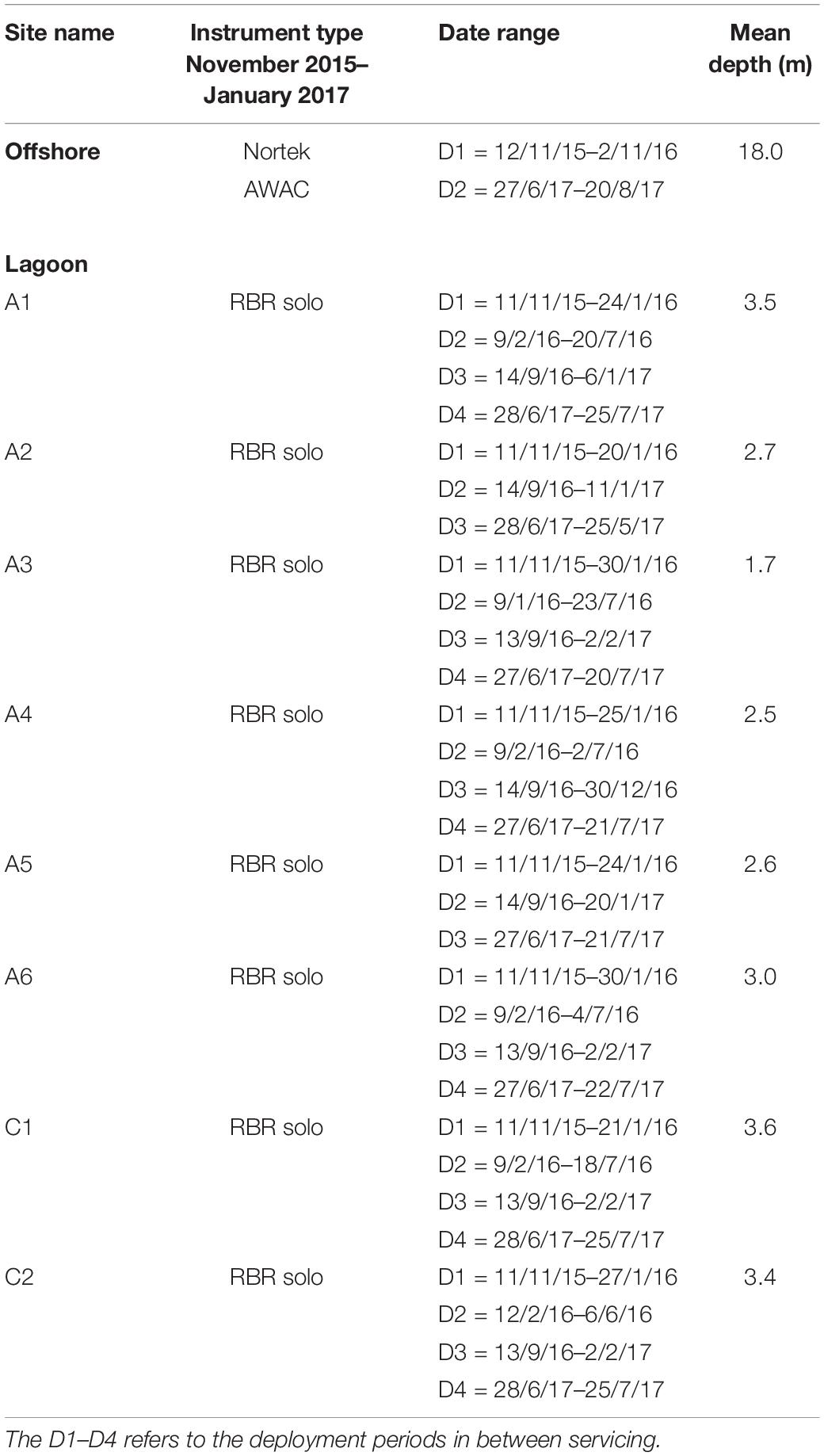
Table 1. Site names, instrument type, and approximate mean depth during the study period.

FIGURE 2

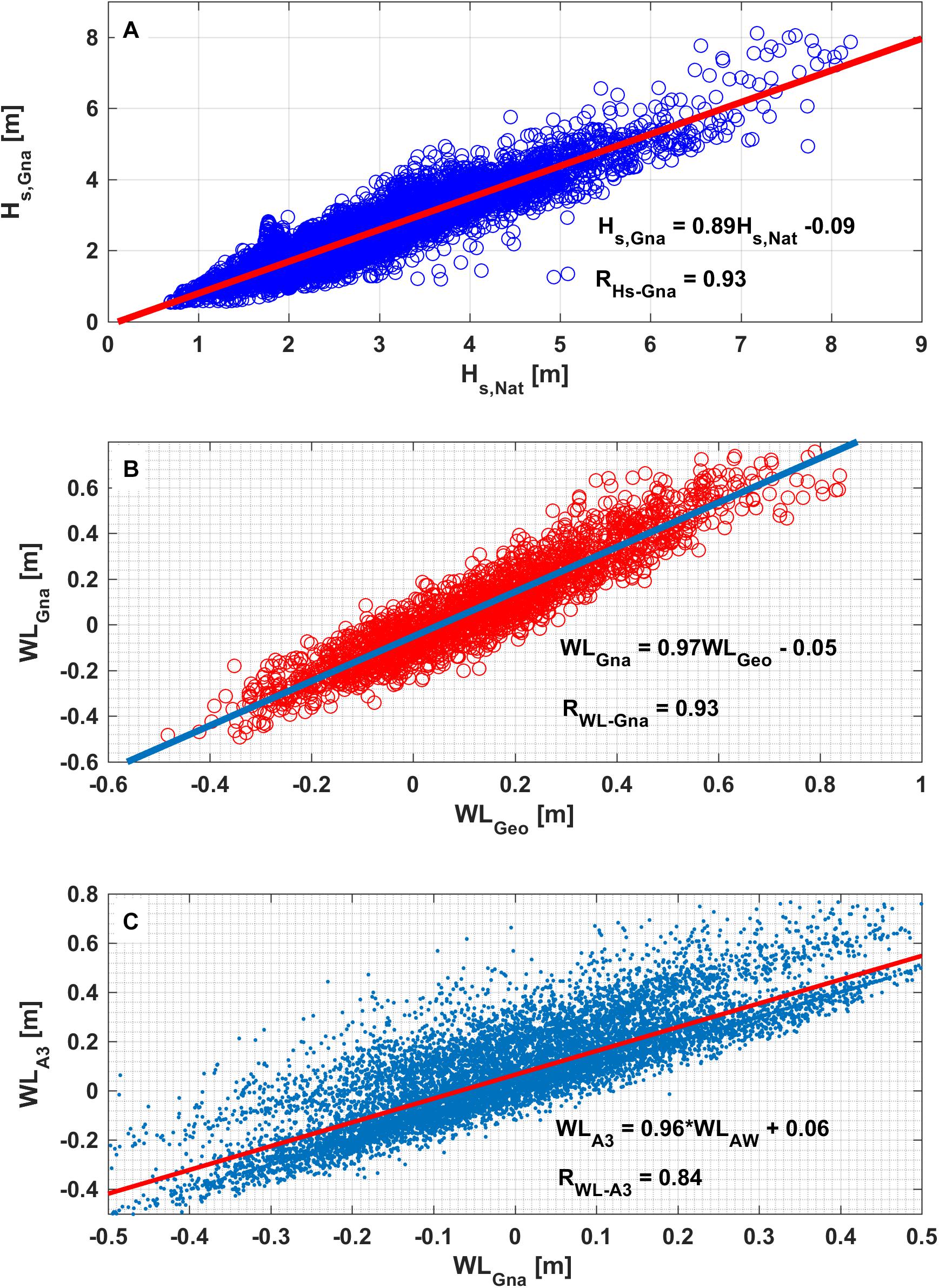
Figure 2. Relationships between (A) offshore wave heights at Cape Naturaliste (H_Nat) and Gnarabup (H_Gna), (B) offshore water level elevations at Busselton (WL_Bus) and Gnarabup beach (WL_Gna), and (C) offshore water level at Gnarabup beach (from AWAC and Busselton tide station) and inside the lagoon at A3.

$H_{s,Gna}=0.8952H_{s,Nat}-0.0978(1)$

where H_s,Gna is offshore wave height at Gnarabup Beach and H_s,Nat is offshore wave height at Cape Naturalist.

Datum-referenced tidal and non-tidal water levels were recorded by a tide gauge operated by DoT located in Port Geographe, approximately 45 km north of the study site. Gaps in the offshore Gnarabup water levels (when the AWAC was not properly functioning or not deployed) were estimated from the Port Geographe tide gauge based on a linear correlation observed between these sites (Figure 2B, R_WL–Gna = 0.93):

$W{L}_{Gna}=0.9753W{L}_{Geo}-0.0515(2)$

where WL_Gna and WL_Geo are water level fluctuations at Gnarabup Beach and Port Geographe, respectively.

Wave statistical properties at the AWAC site were determined based on 2400 sample burst recorded at 1 Hz every other hour. AWAC measurements were processed using the Nortek Storm software, which calculates the wave spectrum based on the acoustically tracked sea surface, pressure fluctuations, and near-surface velocity signals. At the lagoon sites with pressure sensors, spectral estimates of the sea-swell (SS, periods < 25 s) and infragravity (IG, periods 25–600 s) wave height and frequency were made using hourly records (3600 or 7200 samples based on instrument sampling frequency) using linear wave theory. Non-tidal water level variations at frequencies longer than the tides (i.e., subtidal water levels) were obtained by low-pass filtering hourly averaged water level signal using a PL66TN filter with a half-power cutoff period of 33 h (Beardsley et al., 1983). Additionally, wave setup at the lagoon sites was estimated by comparing the depth difference between the sensors located at the reef and the one offshore, as described in e.g., Mory and Hamm (1997) and Beetham et al. (2016),

$\overline{\mathrm{\eta }}=\overline{h}-({\overline{h}}_0+\mathrm{\Delta }h)(3)$

where $\overline{\mathrm{\eta }}$ is the wave setup at the lagoon sites; $\overline{h}$ is the mean depth at the lagoon site; ${\overline{h}}_0$ is the depth at the offshore AWAC (with overbars indicating hourly averaging); and Δh is the difference in elevation between the offshore sensor and the lagoon sensors. The depth difference was calculated assuming a flat sea surface during periods with minimal incident wave energy and periods with small tidal residual (see section “Intertidal Beach Morphology”).

Video Shoreline Detection

At the southern end of the beach, an elevated camera was installed to quantify the shoreline variability. The video system consisted of a Point Gray Blackfly 5 MP video camera with 12.5 mm fixed-focal-length lens that was mounted on a light pole 15.9 m above mean sea level. Every other hour during daylight, the system collected 10 min of video recording at 1.5 Hz. Time exposure (timex) images were produced by averaging the 900 video frames recordings from which the average shoreline position could be extracted (see Holman and Stanley, 2007). Between November 2015 and July 2017, there were 3390 timex images collected by the video system from which ∼97% were useable for shoreline detection.

The timex images were transformed onto a horizontal plane and rectified by taking into account the tidal level to increase the accuracy of the shoreline position on the rectified images (Bryan et al., 2008; Blossier et al., 2017b). Due to the decrease in pixel resolution with increasing distance from the camera, the usable area of the rectified images was 112 m in the cross-shore and 250 m in the alongshore (indicated by the red rectangle on Figure 1A).

Numerous algorithms have been developed to detect shoreline position from timex images automatically (e.g., Uunk et al., 2010; Almar et al., 2012; Simarro et al., 2015). At Gnarabup, the white sand and clear water, coupled with the variability in atmospheric conditions and lighting, resulted in no single methodology from those available in the published literatures working optimally for all images. As a result, we relied on an algorithm that sequentially adopted four methods; the maximum grayscale intensity (Holland et al., 1997), the color channel divergence method that identifies the difference between red and blue channels (Turner et al., 2004), pixel intensity clustering which is based on the hue saturation value (Aarninkhof, 2003), and the Otsu method that works on the black and white color model (Otsu, 1979). Each method was applied to the cross-shore array of pixels of each images and the predicted shorelines from each method were evaluated using a multi-criterion analysis (e.g., Longley et al., 2005).

The shoreline of an image was selected among the four detection methods based on the following criteria. First, the cross-shore difference in the detected shoreline position between adjacent shoreline points was calculated. If the difference between adjacent shoreline points was greater than 5 m, the detected shoreline was automatically discarded. This approach was designed to capture erroneous shorelines in which points of the detected shoreline were either anomalously too far offshore or inland. Second, of the remaining shorelines that were not removed due to the first criterion, the shoreline was selected whose alongshore averaged position was the closest to the alongshore averaged position of a reference shoreline. The reference shoreline was the average shoreline position of a random sampling of 150 hand digitized shorelines spanning all weather conditions. In some cases, often during low light, none of the four automatically detected shorelines met the above criterion, in these cases the shoreline was digitized manually. The multi-criterion analysis showed almost all of the shorelines (∼90%) were predicted using HSV, RGB and grayscale methods (i.e., each method could predict ∼30% of the total shorelines), and the remaining shorelines were predicted using Otsu method. Overall, the combined algorithm was able to accurately detect 76% of the shorelines from the 3277 images, the remaining shorelines required assistance from manual digitization. All of the automatically detected shorelines were also manually checked to ensure their quality.

Intertidal Beach Morphology

As the shoreline recorded from a timex image reflects the position of the waterline with all water level contributions included (tidal and non-tidal), any shoreline position change between successive timex images does not necessarily reflect changes in the beach morphology. To estimate the position of the daily (datum-based) shoreline, the horizontal excursion of the shoreline, in combination with the recorded water levels, were used to reconstruct the intertidal beach morphology. Datum-based water levels recorded by the pressure sensors were estimated by determining the deployment depth of the sensor relative to the Australian Height Datum (AHD, representing approximately mean sea level). This was done by comparing the measured hourly-averaged water levels at site A3, which was close to shore and had the longest recorded time series, with the hourly average water levels recorded at the Port Geographe tide gauge that were referenced to AHD. To minimize the contribution of wave- and/or wind-driven setup and other non-tidal water levels, the comparison was made only for hours when the tidal residuals measured at Port Geographe were less than 0.1 m and the offshore waves recorded by the AWAC were less than 1.5 m. As the deployment location and depth varied slightly between each deployment, this analysis was conducted independently for each deployment period lasting several months. For instances when the water level data was not available from site A3 (e.g., February–June 2017), the water level at that position was estimated from the AWAC water level, given that this water level was found to be well-correlated with the water level measured at A3, R_WL–A3 = ∼0.84 (Figure 2C).

The deployment depth (relative to AHD) for each instrument was estimated from the average bottom elevation (tide removed) from all periods where the tidal residuals and wave heights were less than a threshold (less than 0.1 and 1.5 m, respectively). This resulted in a total of 22 estimates of the instrument depth (with a standard deviation of 0.17 m) for the four deployments (for which the tidal residual ranged from 0.02 to 0.1 m and incident wave height ranged from 0.54 to 1.37 m). The AHD shoreline elevation from each timex image in between November 2015 to July 2017 was assumed to be equivalent to the recorded AHD elevation from the hourly water level at site A3. The daily intertidal beach morphology was then reconstructed by linearly interpolating the horizontal and vertical positions of the hourly shorelines. From the reconstructed beach morphology, the location of the 0 m AHD contour was extracted for each day and used in all subsequent analysis (Figure 3A). This approach was acceptable for 488 of the 504 days. For the remaining 16 days, none of the video derived shorelines spanned the 0 m AHD contour (i.e., water levels never exceeded or dropped below 0 m). For these days, the shoreline position was estimated by extrapolating the beach slope estimated from the range of elevations covered. The regression models used in the beach extrapolation were generated from monthly cross-shore profiles and the corresponding elevations as illustrated in Figure 3B. The modeled curves were used to extend the shape of daily intertidal bathymetry to obtain a shoreline position at a reference elevation (0 m).

FIGURE 3

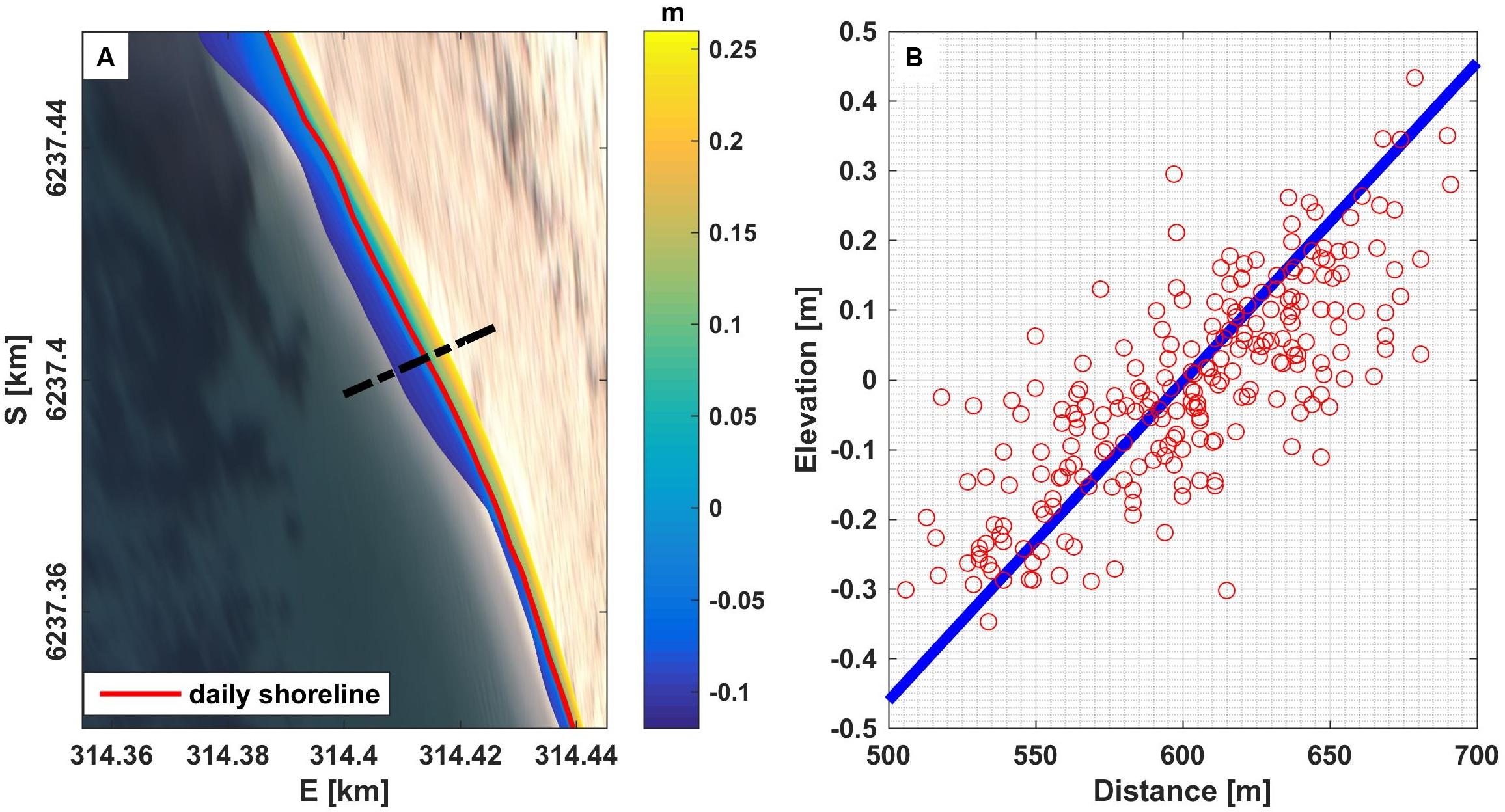
Figure 3. (A) Daily intertidal bathymetry on 16 November 2015, the red line represents the shoreline at 0 m and the dashed black line is the location cross-section profile at (B). (B) A modeled cross-section profile at S 6237.4 km in November 2015 (blue line), red dots are the corresponding shoreline positions recorded during the month.

In addition to the video-derived shorelines, seven topographic beach surveys were conducted between December 2015 and July 2017 using a backpack-mounted Differential Global Navigation Satellite System (DGNSS) receiver. Following the method of Segura et al. (2018), for each survey the complete 1.5 km beach was traversed by foot in a series of cross- and alongshore lines each spaced ∼30 m apart and spanning −0.5 to 5 m AHD. The points from the DGNSS receiver (collected at 2 Hz) were organized into a triangular irregular network (TIN) and subsequently interpolated onto a 2 m regular grid. The sub-aerial beach volume from each survey was estimated using trapezoidal integration (e.g., Roy, 2010) with 2 m grid cell size calculated over 49,485 m² of beach area with −1 m AHD as the lowest elevation. To evaluate the quality of the video derived shorelines we compared the daily 0 m contour shorelines extracted from the video system with those estimated from the DGNSS backpack survey for 4 days during which both data sets were available. The average (across the four surveys) root mean square error (RMSE) calculated over the 250 m alongshore stretch of beach common to both data sets was 1.71 m (average bias of 3.82 m). The difference between the shorelines is potentially a result of image rectification errors (e.g., Tian et al., 2002; Girard, 2018) as well as interpolation of the survey data (to extract the 0 m contour) which was produced from cross-and alongshore transects spaced ∼30 m apart.

Results

Hydrodynamic Conditions

During the study period, the offshore significant sea-swell (SS) wave heights at the offshore AWAC averaged 2.3 m (Figure 4A), with a mean direction from the southwest and west. Wave heights were lower (higher) during the austral summer (winter) months, with episodic, high-energy winter storms causing large wave events (i.e., reaching up ∼8 m in July 2016). From the wave spectrum at the AWAC between November 2015 and July 2017 (Figure 5A) the incident waves were dominated by sea-swell waves with peak period of 5–20 s. We identified 75 days of energetic wave events (daily average H_s higher than 3.5 m) that mainly occurred during winter with maximum daily average H_s of 6.9 m on 31 July 2016. Stormy days also occurred in spring and autumn for example two consecutive days of storm in the beginning of October 2016 (see Figure 4A). The hourly offshore mean water level reached a maximum of 1.05 m above AHD, with a range of 1.62 m over the study period (Figure 4B). The offshore non-tidal water level variations reached a maximum value of up to 0.62 m above AHD and a minimum of −0.17 m AHD. The two reefs shelter the beach creating a semi-protected lagoon, and the daily-averaged significant wave height never exceeded 1.5 m within the lagoon, even when the offshore waves reached 8.4 m (Figure 4D).

FIGURE 4

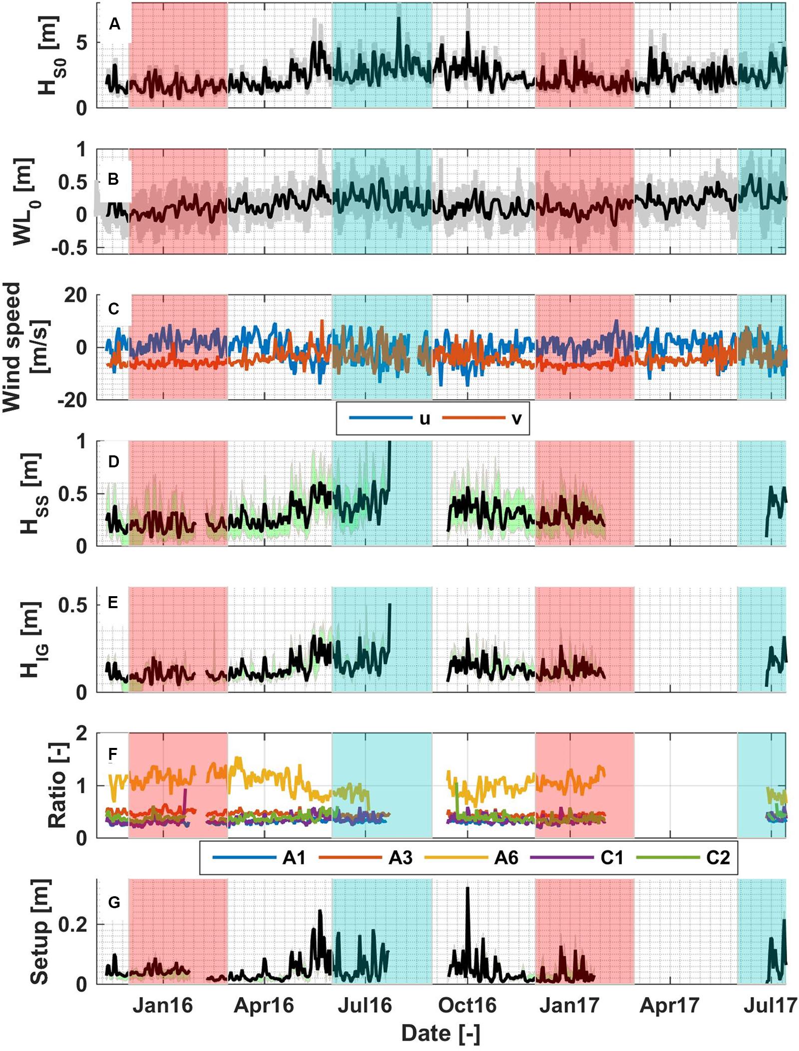
Figure 4. Daily average (solid black line) and hourly (solid gray line) (A) offshore significant wave height. (B) Non-tidal (solid black line, filtered using PL66TN with a half-power cutoff period of 33 h) and hourly water level (solid gray line) variations. (C) East (u, blue line) and north (v, red line) components of daily wind speed. (D) Daily sea-swell (SS) and (E) infragravity (IG) wave heights at site A3, chosen to represent the conditions inside the lagoon. (F) Ratio between IG and SS at selected observation points. (G) Daily wave setup at A3. Gray lines and green areas at figure (D,E,G) denote the range of value among the sensors inside the lagoon. Transparent red and blue regions denote periods of the austral summer and winter, respectively.

FIGURE 5

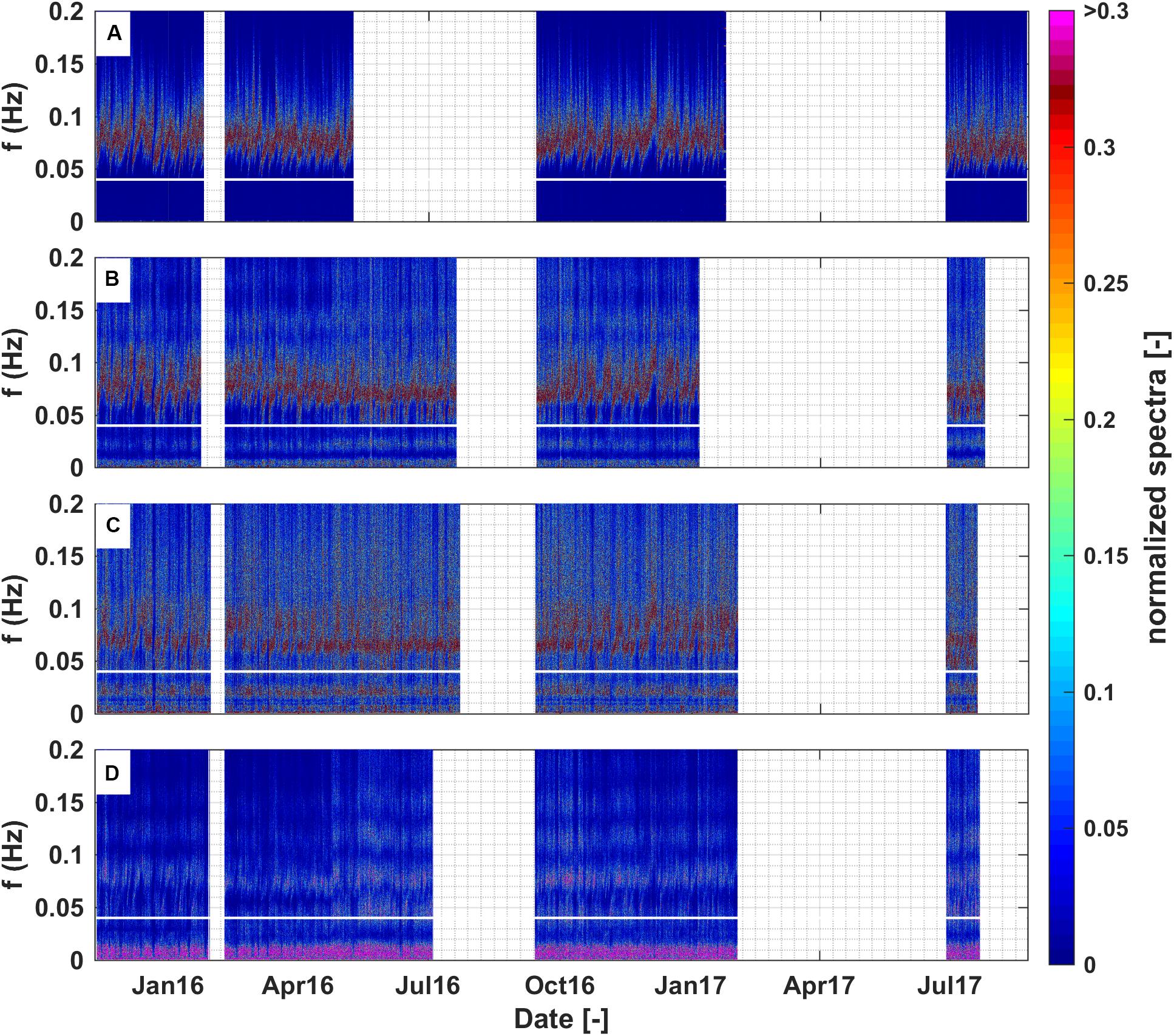
Figure 5. Time series of normalized energy density spectra (against the maximum value of each hourly spectra) at (A) offshore, (B) A1, (C) A3, and (D) A6 (see Figure 1A for site descriptions) with spectra resolution of 0.0005 Hz. The horizontal white line on the figures represents the separation frequency (fsplit of 0.04 Hz) for the short-wave and infragravity bands. Blank parts on the figures denote the periods without observation.

Inside the lagoon, as wave energy within the SS band dissipated, the wave spectrum became increasingly dominated by IG waves, particularly at site A6 in the protected southern corner of the lagoon (see Figures 5B–D). Similar to other reef environments, SS waves were mostly depth-limited in the lagoon (Lowe et al., 2009) with the breaking index (the ratio between wave height and local water depth) of ∼0.4 for all sites (Figure 6A). In contrast, the IG waves in the lagoon did not appear to display any depth limitation on water depth over the study period (Figure 6B). The IG waves were typically less than 0.5 m and showed less spatial variability among sensors inside the lagoon (Figure 4E). Within the lagoon, the IG waves made a significant contribution to the total wave energy, especially at the most protected area at the south (site A6) where the SS waves were smallest (Figure 4F). Both the SS and IG wave heights were strongly correlated with the offshore waves (R_SS = 0.83 and R_IG = 0.81, respectively).

FIGURE 6

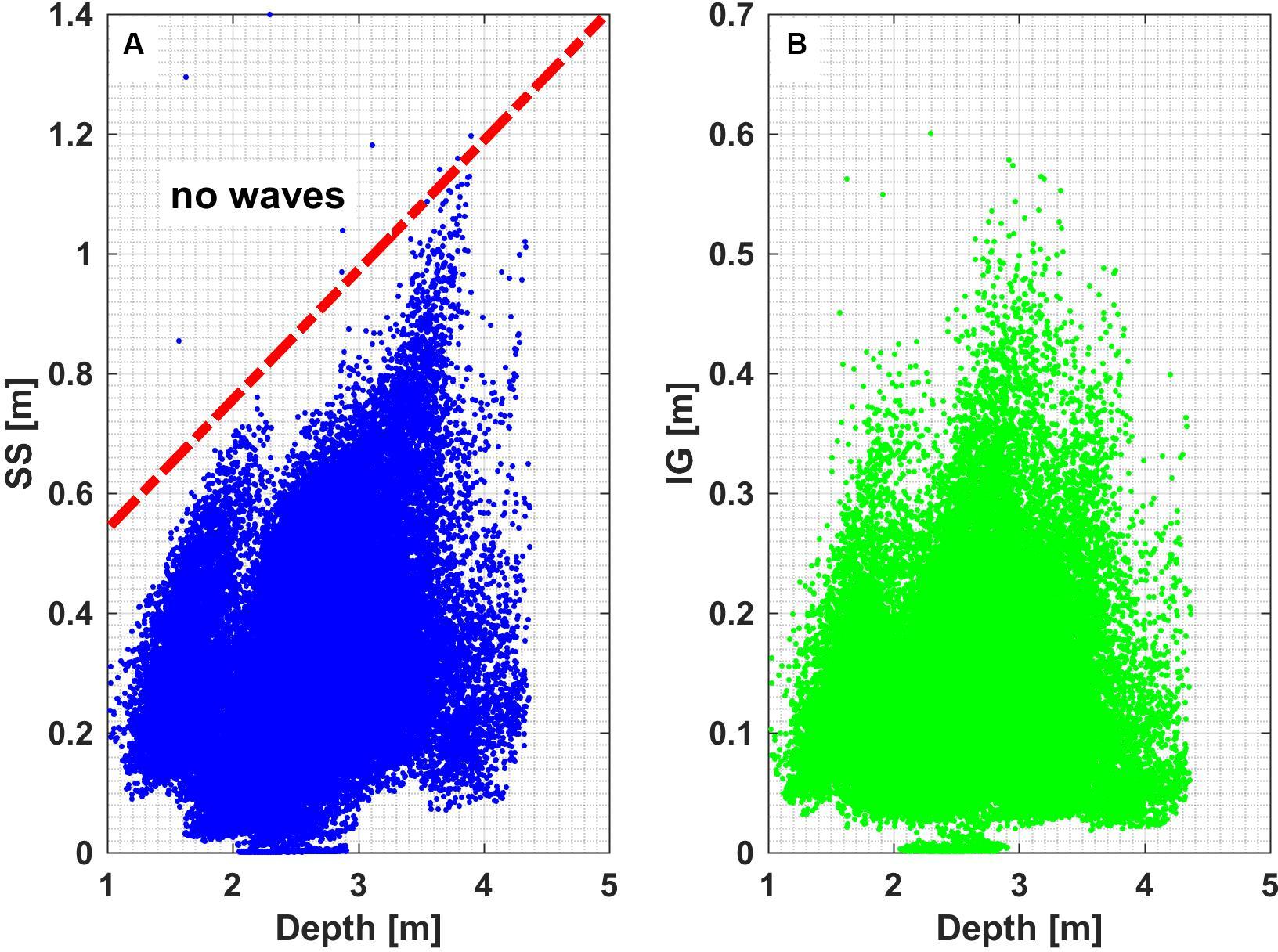
Figure 6. Correlation between water depth and (A) sea-swell significant wave heights as well as (B) infragravity significant wave heights at all observed points inside the lagoon. The red dashed line in (A) represents a sea-swell wave height to depth ratio (γ) of 0.39.

Time-series of wave setup at site A3 are shown in Figure 4G. Note that there were only small differences in setup between A3 and the other lagoon sites. This is likely because the setup in the lagoon was dictated by breaking on the offshore reefs rather than breaking inside the lagoon, with maximum RMSE among sites relative to A3 of only 0.016 m with maximum bias of less than 1 cm (% error among sites relative to A3 of 7.7–31.5%, highest at A1) over the study period (not shown). The maximum daily wave setup over the 15 months (November 2015 to January 2017) reached 0.32 m at site A3, which coincided with a large wave event on 1 October 2016 when the daily significant wave height at the AWAC site was 5.8 m. Wave setup at all sites was very strongly correlated (R_η of ∼0.85 to ∼0.95) with the off-shore wave height squared (proportional to the incident wave energy) (Table 2).

TABLE 2

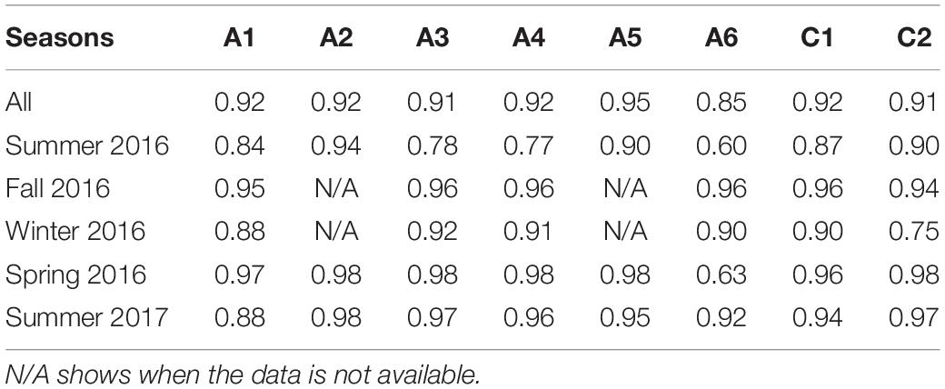
Table 2. Summary of correlation coefficient between offshore wave energy (∼H²) and setup at observed locations for all observation period and every season.

Beach Dynamics

Sub-aerial beach dynamics were quantified using the daily video-derived shorelines, which supplemented by less frequent DGNSS backpack-based surveys of the entire 1.5 km beach. While the video-derived shorelines were available almost every day, they only captured the southern 250 m of the beach. As a result, the complete topographic surveys of the beach, while being much less frequent, provide valuable additional context to the video shorelines.

Topographic Beach Surveys

Over the 20 months (from December 2015 to July 2017), the total sub-aerial beach volume averaged over the entire 1.5 km beach was largely conserved (Figure 7A, the blue line). Relative to the initial total beach volume (in December 2015) of ∼195,000 m³ (calculated over 49,485 m² of beach area with −1 m AHD as the lowest elevation), the maximum total beach volume changes were ∼23,100 m³ (∼15.4 m³/m), which is equivalent to ∼11.8% of the total initial beach volume (Figure 7A). However, despite the total beach volume being mostly conserved, there was considerable alongshore variability in the seasonal erosion and accretion patterns over the study period (Figure 8).

FIGURE 7

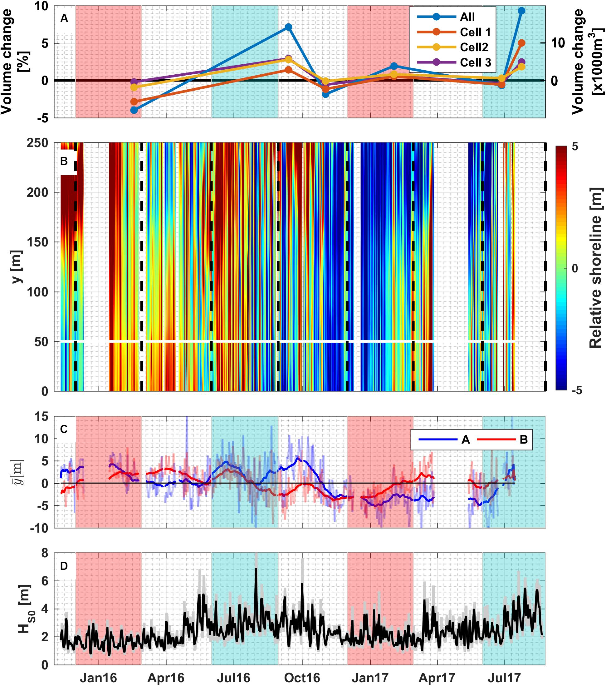
Figure 7. (A) Volume change of the beach between successive topographic surveys in 2015–2017, relative to the initial beach volume in December 2015. The respective primary and secondary y-axis show the beach volume change in percentage relative to initial total beach volume and in 1000 cubic meters. (B) Daily shoreline positions (colors) relative to the mean position over the entire observation period along the 250 m alongshore stretch of beach. A white horizontal line shows the boundary between Cell 3A and B. (C) Daily (thin) and monthly averaged (bold) shoreline positions at 5 m farthest points from the node of part (A) (blue) and (B) (red) which refer to dashed red lines at Figure 1B. Gaps in (B,C) are the periods when video images were unavailable. (D) Daily average (solid black line) and hourly (solid gray line) offshore significant wave height. Transparent red and blue regions as the vertical black dashed lines denote periods of the austral summer and winter, respectively.

FIGURE 8

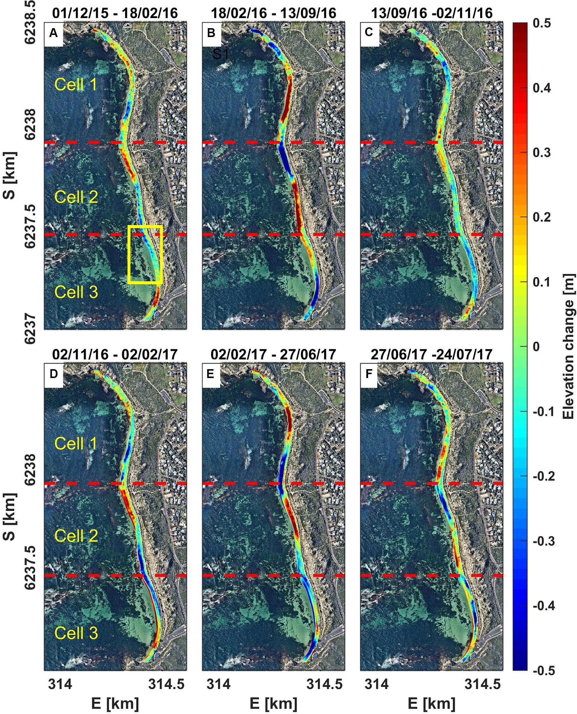
Figure 8. Beach elevation changes within period of (A) 01/12/2015-18/02/2016, (B) 18/02/2016-13/09/2016, (C) 13/09/2016-02/11/2016, (D) 02/11/2016-02/02/2017, (E) 02/02/2017-27/06/2017, (F) 27/06/2017-24/07/2017, separated into three cells (Cell 1-Cell 3) based on the position of anti-nodes located behind the offshore reefs (red-dashed lines). The yellow box in figure (A) is the area covered by video camera system.

To investigate these erosion/accretion patterns in further detail, we divided the beach into three cells based on the patterns in the beach elevation changes (Figure 8, with boundaries generally aligning with the alongshore locations of the reefs). The volume changes indicate that each cell is semi-closed, as evident by small volume within Cell 1 to Cell 3 in Figure 7A, with a local out of phase erosion/accretion response within each cell (Figure 8). The elevation changes over the two summer seasons within the study period (Figures 8A,D) showed similar patterns, characterized by sand deposition at the northern and southern corners of the beach, accretion of the salient that formed where the northern reef attaches to the coast at the boundary between Cell 1 and 2, and erosion of the salient that formed where the southern reef attaches to the coast at the boundary between Cell 2 and 3.

The beach evolution in transitional seasons (spring and autumn), showed different behavior. During spring between September to November 2016 (Figure 8C), both the northern salient (boundary between Cell 1 and 2) and the corners of the beach near the headlands accreted; whereas the southern salient (boundary between Cell 2 and 3) eroded. The sand volume during the period decreased by ∼3,500 m³ (around −2.4 m³/m or −1.8% of total beach volume, Figure 7A), which is likely related to the high wave heights in October to November 2016 that reached 5.8 m (see Figure 7D). In contrast, between February to June (autumn) 2017, the beach exhibited erosion at both salients and deposition at all embayments (Figure 8E). The autumn profile showed a slight decrease (−0.87%) of the total beach volume (Figure 7A). During autumn 2017, the daily wave heights were relatively higher (average of 2.3 m), compared to that of the summer (average of 2.1 m).

The winter (June to August) beach elevation patterns (Figures 8B,F) showed an opposite response to the summer patterns (Figures 8A,D). Sediment accumulated in the southern portion of each cell, with erosion on the northern ends; during this period there was additional ∼18,000 m³ (9.3%) of sand added to the overall beach volume, mostly deposited on the lower beach between 0 and −1 m elevations, thus indicating some flattening of the beach.

Video Shoreline Observations

The video monitoring captured daily shoreline movements in the central and northern portion of Cell 3 where images were obtained (see Figure 1A, red box). Consistent with the topographic surveys, the video observations indicated shoreline rotation within Cell 3, and we thus used the nodal point (derived from the topographic beach surveys) to divide the cell into two sections within the camera’s field of view (hereinafter referred to Cell 3A and Cell 3B, Figure 1B, note the camera’s field of view only captured the northern portion of Cell 3B close to the nodal point). The temporal mean shoreline position averaged over the 20 month period was removed from the daily shoreline position yielding daily relative shoreline positions (Figure 7B). The shoreline movements were characterized by short term oscillations over days-to-weeks, which were superimposed on longer time-scale (seasonal) cycle (Figures 7B,C). Given that the data from the topographic surveys indicated that similar beach rotation patterns occurred over the entire beach (Figure 8), we would expect both Cells 1 and 2 to show rotational responses that were similar to Cell 3.

The shoreline rotation signal within Cell 3 becomes even more apparent (Figure 7C) within timeseries of the monthly-averaged northern and southern limits of the shoreline positions within the cell. In the rectified images, these locations coincide with y = 0–5 m (Cell 3B) and y = 245–250 m (Cell 3A) (see red dashed lines in Figure 1B). The offshore wave and water level conditions (Figure 4) influenced the change of shoreline positions, resulting in both an in-phase (uniform) and out-phase (rotational) response at the extreme ends of Cell 3A and Cell 3B (Figure 7C). In December 2015–February 2016 (summer), the wave energy was the lowest of all the seasons over the study period (with daily H_s0 of 1.6 m on average), and the shoreline across both Cells 3A and 3B was accreted (except for in the very early summer where Cell 3B was eroded), with larger accretion in Cell 3A suggesting northward alongshore transport (Figure 7C). In December 2016–February 2017 (Summer), most of the shoreline was consistently eroded across both Cells 3A and B with greater erosion at Cell 3A (∼−4 m) compared to that of Cell 3B, which could be due to some southward alongshore sediment transport. The subtle differences in the shoreline responses during the summers of 2016 and 2017 appears to be due to the differences in the average offshore wave conditions between these years. Compared to the summer of 2016, the summer of 2017 experienced larger waves (average H_s of 2.1 m versus 1.6 m in the summer of 2016). This could be partially attributed to stronger local wind conditions in 2017 (average of 7.7 m/s) than the average value of 7.0 m/s in 2016 (Figures 4A,C).

During the winter (June–August) seasons, the shoreline responded more consistently at Cells 3A and 3B, with both sub-cells showing rapid erosion and recovery (Figures 7B,C). The shorelines showed a slight counter-clockwise rotation at the beginning of the winter of 2016 and then demonstrated an in-phase (uniform) response during the remainder of the winter of 2016 before the shoreline began to rotate counter-clockwise after July 2016 (Figures 7B,C).

The shoreline patterns in autumn (March–May) were opposite to that of spring (August–November) in which during both periods, the daily offshore wave height was moderate (2–4 m). Shoreline patterns in autumn 2016 showed the shoreline rotated clockwise, in which Cell 3B was more accreted than Cell 3A. However, during spring (around September to early-October 2016), when the daily wave heights decreased, the sediment tended to move back to Cell 3A; as a result, Cell 3B became eroded and the shoreline rotated anti-clockwise (Figure 7C).

During large wave events (defined as days with offshore H_s > 3.5 m), which mainly occurred during winter months but also occasionally in other seasons (Figure 4A), the entire shoreline in Cell 3 mostly retreated up to 10 m. But it often quickly recovered as wave energy decreased; for example, during the storms on 31 July 2016 with average daily offshore wave height of 5.8 m (Figure 4A). During some storm events, we observed a rotational response, i.e., accretion within one portion of Cell 3 while the other portion became eroded; however, there were inconsistent responses in shoreline rotation to individual storms. Examples include the days of 16 May (H_s = 5 m) and 7 June 2016 (H_s = 4.6 m) where Cell 3A accreted, whereas on 15 March (H_s = 4.6 m) and 13 July 2017 (H_s = 4.6 m) Cell 3B accreted. Over the full record correlations between Hs > 3.5 m and shoreline at 3A–3B were very weak with R < 0.1 (p > 0.05).

The shoreline positions during the observation period were very weakly correlated to the main offshore hydrodynamic forcing, including wave height and direction as well as subtidal water level (that modulates wave transmission across the reefs) (| R| < 0.3, p < 0.05). However, if the correlations were computed between the shoreline positions and wave heights from each season independently, we found greater correlations. This especially occurred during summer and winter, with R = −0.55 and −0.48 at Cell 3A as well as R = −0.55 and −0.42 at Cell 3B (with all p < 0.05), respectively. Similarly, correlation coefficients with the offshore water level were larger in summer (Cell 3A of ∼0.26 and Cell 3B of ∼0.37, all p < 0.05) but slightly weaker in winter (Cell 3A of 0.16 p > 0.05 and Cell 3B of 0.32 with p < 0.05). During transitional seasons, autumn and spring, the shoreline positions were weakly correlated with the offshore hydrodynamics. Correlations remained low between shoreline position and offshore wave direction over the entire data set or by seasons (R < 0.14 for entire years and seasonal, p < 0.05 at Cell 3A for all years and spring). Although there were appreciable fluctuations in the shoreline position at individual locations, overall, there was a balance between erosion and accretion indicating the beach is in dynamic equilibrium with no significant net trend in erosion or accretion (Figure 7B).

Given the role of offshore water level in modulating wave breaking over reef platforms (e.g., Lowe et al., 2005), it is expected that the offshore water level fluctuations at the site would have an impact on the shoreline dynamics. To examine the shoreline response to both offshore waves and water levels, the shoreline position from the northern and southern 5 m of the camera’s field of view (transparent lines in Figure 7C) were organized into 0.2 m bins of daily averaged offshore wave height and 0.1 m bins of daily averaged offshore water level. All daily shoreline positions that occurred with the corresponding wave and water level bins were averaged within each bin (Figure 9). While there was significant scatter, in general, we see a trend of greater erosion for the same wave height, with lower water level, and vice-versa. The greatest shoreline accretion occurred at the higher water levels. For example, in both Cells 3A and B for offshore wave heights between 2 and 2.5 m, we generally observed shoreline accretion during high water levels and erosion for low water levels. By further relating the erosion and accretion patterns of Cell 3A and B to larger offshore wave heights (>3.5 m) and the corresponding subtidal water levels across study period, we found that accretion at both Cells 3A and B mostly occurred during high subtidal water levels (average of 0.32 m); for example, on 1 October 2016 (daily H_s ∼5.8 m and subtidal water level ∼0.3 m). In contrast, when the subtidal water level was lower (average of 0.21 m), erosion occurred across the entire shoreline, for example, on 9 August 2016 (daily H_s ∼4.2 m and subtidal water level ∼0 m). During intermediate subtidal water levels (in between 0.21 and 0.32 m), we identified a rotational response with accretion at one of the cell followed by erosion at the other cell.

FIGURE 9

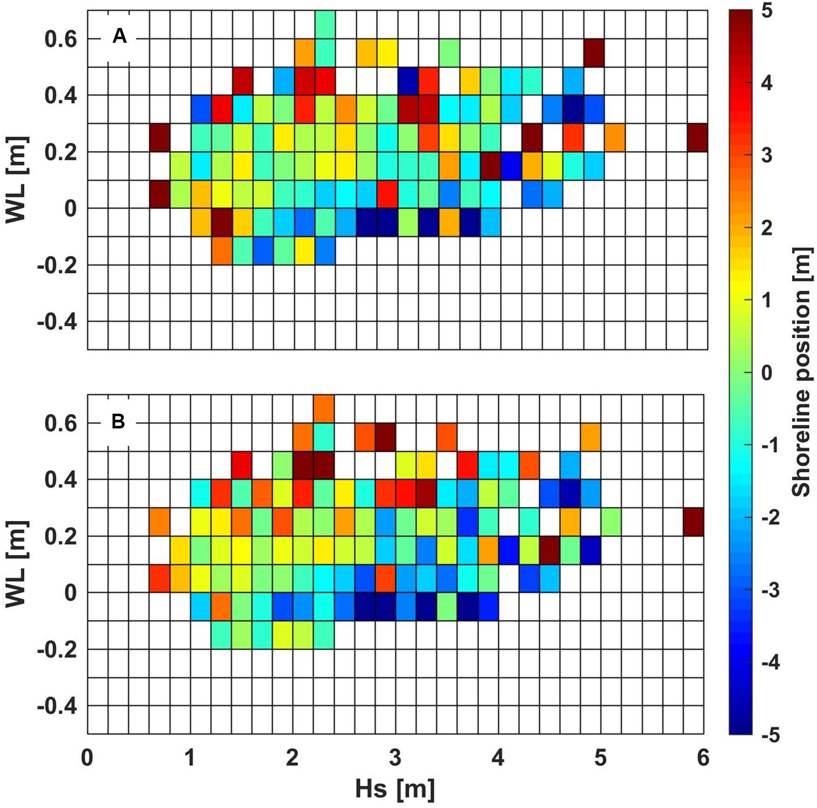
Figure 9. Offshore subtidal water level (bin size 0.1 m, y-axis) and significant wave height (bin size 0.2 m, x-axis) compared to average shoreline positions at (A) Cell 3A and (B) 3B. The colors denote to the averaged shoreline position of all daily shorelines within each respective bin or the shoreline position in the event only one daily shoreline position fell within a bin.

Discussion

This study investigated the shoreline and beach elevation changes at a reef fronted pocket beach at Gnarabup Beach in southwestern Australia. The site receives substantial offshore wave energy. Strong wave breaking occurs over the reefs, where significant energy is generated at the infragravity frequencies. Infragravity waves contribute to a large portion of the total wave energy inside the lagoon, similar to what has been found at coral reef sites (e.g., Taebi et al., 2011; Torres-Freyermuth et al., 2012; Péquignet et al., 2014). The site also features substantial seasonal non-tidal water level variability, with fluctuations which can be as large as the tide.

At Gnarabup Beach, seasonal shoreline changes mostly consisted of beach rotation with differing areas of the 1.5 km pocket beach experiencing in and out of phase patterns of erosion and accretion represented by beach surveys (Figures 7A, 8) and also the video analysis (Figures 7B,C). The video derived shorelines for the southern portion of the beach showed considerable temporal and spatial variability. Similar to the research conducted by Norcross et al. (2002) at a reef-fringed pocket beach in Hawaii, we also found weak bivariate correlations between the observed hydrodynamic forcing (waves and water levels) and shoreline position. This was potentially caused by the complexity of beach geometry whereby the presence of the reefs and headlands caused a non-linear response of the shoreline to the offshore forcing. As such, the video records indicate the shoreline positions had no consistent relationship with the offshore forcing conditions (see Figure 9). While in many cases the shoreline was in an eroded state during low subtidal water level, we also found during larger wave events (>3.5 m) the shorelines showed variable erosion and accretion patterns at different subtidal water levels. Considering Gnarabup beach is a pocket beach with minimum sediment exchange between the beach and adjacent areas; the shoreline accretion (instead of the expected erosion) at all of the sub-regions during larger wave events could be explained as follows. Energetic waves with high subtidal water level occurring mainly during winter would likely contribute to beach flattening and/or dune erosion as the waves erode a higher part of the beach and further deposited the eroded material seaward. As evidence of that, beach topography surveys collected around winter indicated additional sand within the system instead of erosion (see Figure 7A), which could have potentially come from the upper beach area. Evidence of beach flattening is also seen in the topographic beach surveys in Cell 3 (blue color in Figures 8D,F), where the upper part of the beach was eroded.

The patterns of beach erosion and recovery, as observed in both the beach surveys and video shoreline data, indicate that seasonal beach rotation occurs within the study area. This is similar to what was found by Jeanson et al. (2013) for another reef fronted pocket beach. Instead of the whole beach rotating in a pattern that commonly occurs in pocket beaches (e.g., Ranasinghe et al., 2004; Castelle and Coco, 2012; Do et al., 2016), at this reef-fringed pocket beach the rotation occurred in clusters (cells). This is associated with the presence of offshore fringing reefs that partly connected to the shore, creating quasi-headlands within the pocket beach that could partially-impede the alongshore sediment transport.

Furthermore, the existence of fringing reefs creates a narrow offshore gap, i.e., the width between the southern headland and the southern fringing reefs is only ∼230 m, protecting the beach which can likely explain why the beach was not very sensitive to changes in the wave direction. While literature on open-coast beaches has often identified a strong influence of offshore wave direction on shoreline rotational response (e.g., Turki et al., 2013; Daly et al., 2015; Luccio et al., 2019), at Gnarabup beach the beach rotation was more strongly controlled by the interaction between the offshore hydrodynamic conditions and the reef morphology.

Conclusion

A series of field observations over 20 months were used to assess the behavior of an embayed pocket beach fringed by rocky reefs in southwestern Australia. Despite the high incident wave energy at the site, most of the incoming wave energy was dissipated by the shallow reefs, resulting in relatively low wave energy conditions along the shoreline. Seasonal beach surveys over the entire 1.5 km of the beach and daily video derived shorelines over the southern 250 m of beach indicate the shoreline shows both patterns of rotation as well as uniform erosion and accretion. Over the entire study period, the beach experienced large (up to 10 m) erosion caused by storms, yet, the erosion events were quickly followed by recovery that caused the shoreline position was largely stable. The video derived daily shorelines also reveal differing shoreline response based on the combination of offshore waves and water levels (which vary as a result of seasonal variations in the Leeuwin Current). In general, at comparable wave height conditions, the beach tended to be more eroded during low water levels compared to during high water levels. This pattern, while somewhat counterintuitive, may have resulted from both beach flattening and rotation of the shoreline. The study shown the complexity of beach dynamics within a reef-fringed pocket beach whereby the wave energy at the shoreline is strongly modulated by offshore wave conditions but also reef submergence.

Data Availability Statement

The datasets used in this study are available on request to the corresponding author.

Author Contributions

JR conducted beach morphology surveys, analysis of the video imagery and wrote the initial draft of the manuscript. JH conducted the in situ deployments and analysis, installed the video system, and assisted JR in the writing of the manuscript. RL and DR assisted in the data interpretation in a writing of the manuscript.

Funding

This work was supported by the Western Australia Department of Transport, Shire of Augusta Margaret River, and Australia Awards Scholarship.

Conflict of Interest

The authors declare that the research was conducted in the absence of any commercial or financial relationships that could be construed as a potential conflict of interest.

Acknowledgments

The authors are grateful to Peter Kovesi and Karin Bryan for fruitful discussions and the help on the video rectification, also Carlin Bowyer, Anton Kuret, and Rebecca Green for assisting with the field experiments.

References

Aarninkhof, S. G. J. (2003). Nearshore Bathymetry Derived From Video Imagery. Delft: TU Delft.

Google Scholar

Almar, R., Ranasinghe, R., Senechal, N., Bonneton, P., Roelvink, D., Bryan, K. R., et al. (2012). Video-based detection of shorelines at complex meso–macro tidal beaches.(Report). J. Coast. Res. 28, 1040–1048. doi: 10.2112/jcoastres-d-10-00149.1

CrossRef Full Text | Google Scholar

Baldock, T. E. (2012). Dissipation of incident forced long waves in the surf zone—Implications for the concept of “bound” wave release at short wave breaking. Coast. Eng. 60, 276–285. doi: 10.1016/j.coastaleng.2011.11.002

CrossRef Full Text | Google Scholar

Beardsley, R. C., Mills, C. A., Rosenfeld, L. K., Bratkovich, A. W., Erdman, M. R., Winant, C. D., et al. (1983). CODE-1: Moored Array and Large-Scale Data Report. Woods Hole, MA: Woods Hole Oceanographic Institution.

Google Scholar

Becker, J. M., Merrifield, M. A., and Yoon, H. (2016). Infragravity waves on fringing reefs in the tropical pacific: dynamic setup. J. Geophys. Res. Oceans 121, 3010–3028. doi: 10.1002/2015jc011516

CrossRef Full Text | Google Scholar

Beetham, E., Kench, P. S., O’ Callaghan, J., and Popinet, S. (2016). Wave transformation and shoreline water level on funafuti atoll. Tuvalu. J. Geophys. Res. Oceans 121, 311–326. doi: 10.1002/2015jc011246

CrossRef Full Text | Google Scholar

Blossier, B., Bryan, K. R., Daly, C. J., and Winter, C. (2017a). Shore and bar cross-shore migration, rotation, and breathing processes at an embayed beach. J. Geophys. Res. Earth Surface 122, 1745–1770. doi: 10.1002/2017jf004227

CrossRef Full Text | Google Scholar

Blossier, B., Bryan, K., Daly, C., and Winter, C. (2017b). Spatial and temporal scales of shoreline morphodynamics derived from video camera observations for the island of Sylt, German Wadden Sea. Geo Mar. Lett. 37, 111–123. doi: 10.1007/s00367-016-0461-7

CrossRef Full Text | Google Scholar

Bryan, K. R., Salmon, S. A., and Giovanni, C. (2008). “Measuring storm run-up on intermediate beaches using video,” in Coastal Engineering ed. J. M. Smith (Singapore: World Scientific Publishing), 854–864.

Google Scholar

Buckley, M. L., Lowe, R. J., Hansen, J. E., Van Dongeren, A. R., and Storlazzi, C. D. (2018). Mechanisms of wave-driven water level variability on reef-fringed coastlines. J. Geophys. Res. Oceans 123, 3811–3831. doi: 10.1029/2018JC013933

CrossRef Full Text | Google Scholar

Castelle, B., and Coco, G. (2012). The morphodynamics of rip channels on embayed beaches. Cont. Shelf Res. 43, 10–23. doi: 10.1016/j.csr.2012.04.010

CrossRef Full Text | Google Scholar

Daly, C. J., Bryan, K. R., and Winter, C. (2014). Wave energy distribution and morphological development in and around the shadow zone of an embayed beach. Coast. Eng. 93, 40–54. doi: 10.1016/j.coastaleng.2014.08.003

CrossRef Full Text | Google Scholar

Daly, C. J., Winter, C., and Bryan, K. R. (2015). On the morphological development of embayed beaches. Geomorphology 248, 252–263. doi: 10.1016/j.geomorph.2015.07.040

CrossRef Full Text | Google Scholar

Dehouck, A., Dupuis, H., and Sénéchal, N. (2009). Pocket beach hydrodynamics: the example of four macrotidal beaches, Brittany, France. Mar. Geol. 266, 1–17. doi: 10.1016/j.margeo.2009.07.008

CrossRef Full Text | Google Scholar

Do, K., Kobayashi, N., Suh, K.-D., and Jae-Youll, J. (2016). Wave transformation and sand transport on a macrotidal pocket beach. J. Waterway PortCoast. Ocean Eng. 142:04015009. doi: 10.1061/(ASCE)WW.1943-5460.0000309

PubMed Abstract | CrossRef Full Text | Google Scholar

Feng, M., Meyers, G., Pearce, A., and Wijffels, S. (2003). Annual and interannual variations of the leeuwin current at 32°S. J. Geophys. Res. Oceans 108:3555. doi: 10.1029/2002jc001763

CrossRef Full Text | Google Scholar

Ford, M., Becker, J., and Merrifield, M. (2013). Reef flat wave processes and excavation pits: observations and implications for majuro atoll. Marshall Islands. J. Coast. Res. 29, 545–554. doi: 10.2112/jcoastres-d-12-00097.1

CrossRef Full Text | Google Scholar

Girard, C. M. (2018). Processing of Remote Sensing Data. Boca Raton, FL: CRC Press.

Google Scholar

Gourlay, M. R., and Colleter, G. (2005). Wave-generated flow on coral reefs—an analysis for two-dimensional horizontal reef-tops with steep faces. Coast. Eng. 52, 353–387. doi: 10.1016/j.coastaleng.2004.11.007

CrossRef Full Text | Google Scholar

Hardy, T. A., and Young, I. R. (1996). Field study of wave attenuation on an offshore coral reef. J. Geophys. Res. Oceans 101, 14311–14326. doi: 10.1029/96jc00202

CrossRef Full Text | Google Scholar

Harley, M. D., Turner, I. L., Short, A. D., and Ranasinghe, R. (2011). A reevaluation of coastal embayment rotation: the dominance of cross-shore versus alongshore sediment transport processes, Collaroy-Narrabeen Beach, southeast Australia. J. Geophys. Res. Earth Surface 116:F04033. doi: 10.1029/2011JF001989

CrossRef Full Text | Google Scholar

Holland, K. T., Holman, R. A., Lippmann, T. C., Stanley, J., and Plant, N. (1997). Practical use of video imagery in nearshore oceanographic field studies. Oceanic Eng. IEEE J. 22, 81–92. doi: 10.1109/48.557542

CrossRef Full Text | Google Scholar

Holman, R. A., and Stanley, J. (2007). The history and technical capabilities of Argus. Coast. Eng. 54, 477–491. doi: 10.1016/j.coastaleng.2007.01.003

CrossRef Full Text | Google Scholar

Horta, J., Oliveira, S., Moura, D., and Ferreira, Ó (2018). Nearshore hydrodynamics at pocket beaches with contrasting wave exposure in southern Portugal. Estuar. Coast. Shelf Sci. 204, 40–55. doi: 10.1016/j.ecss.2018.02.018

CrossRef Full Text | Google Scholar

Jeanson, M., Anthony, E. J., Dolique, F., and Aubry, A. (2013). Wave characteristics and morphological variations of pocket beaches in a coral reef–lagoon setting. Mayotte Island, Indian Ocean. Geomorphology 182, 190–209. doi: 10.1016/j.geomorph.2012.11.013

CrossRef Full Text | Google Scholar

Longley, P., Goodchild, M., Maguire, D., and Rhind, D. (2005). “New developments in geographical information systems: principles, techniques, management and applications,” in Geographical Information Systems: Principles, Techniques, Management and Applications, 2nd Edn. Abridged, eds P. Longley, M. Goodchild, D. Maguire and D. Rhind (New Jersey, United States: John Wiley & Sons Inc), 404.

Google Scholar

Lowe, R. J., and Falter, J. L. (2015). Oceanic forcing of coral reefs. Annu. Rev. Mar. Sci. 2015, 43–66. doi: 10.1146/annurev-marine-010814-015834

PubMed Abstract | CrossRef Full Text | Google Scholar

Lowe, R. J., Falter, J. L., Atkinson, M. J., and Monismith, S. G. (2009). Wave-driven circulation of a coastal reef-lagoon system. J. Phys. Oceanogr. 39, 873–893. doi: 10.1175/2008jpo3958.1

CrossRef Full Text | Google Scholar

Lowe, R. J., Falter, J. L., Bandet, M. D., Pawlak, G., Atkinson, M. J., Monismith, S. G., et al. (2005). Spectral wave dissipation over a barrier reef. J. Geophys. Res. Oceans 110:C04001. doi: 10.1029/2004jc002711

CrossRef Full Text | Google Scholar

Luccio, D. D., Benassai, G., Paola, G. D., Mucerino, L., Buono, A., Rosskopf, C. M., et al. (2019). Shoreline rotation analysis of embayed beaches by means of in situ and remote surveys. Sustainability 11:725. doi: 10.3390/su11030725

CrossRef Full Text | Google Scholar

Masselink, G., Russell, P., Coco, G., and Huntley, D. (2004). Test of edge wave forcing during formation of rhythmic beach morphology. J. Geophys. Res. 109. doi: 10.1029/2004jc002339

CrossRef Full Text | Google Scholar

Monismith, S., Herdman, L., Ahmerkamp, S., and Hench, J. (2013). Wave transformation and wave-driven flow across a steep coral reef. J. Phys. Oceanogr. 43, 1356–1379. doi: 10.1175/jpo-d-12-0164.1

CrossRef Full Text | Google Scholar

Mory, M., and Hamm, L. (1997). Wave height, setup and currents around a detached breakwater submitted to regular or random wave forcing. Coast. Eng. 31, 77–96. doi: 10.1016/S0378-3839(96)00053-1

CrossRef Full Text | Google Scholar

Norcross, Z. M., Fletcher, C. H., and Merrifield, M. (2002). Annual and interannual changes on a reef-fringed pocket beach: kailua Bay. Hawaii. Mar. Geol. 190, 553–580. doi: 10.1016/S0025-3227(02)00481-4

CrossRef Full Text | Google Scholar

Otsu, N. (1979). A threshold selection method from gray-level histograms. IEEE Trans. Syst. Man. Cybernet. 9, 62–66. doi: 10.1109/tsmc.1979.4310076

CrossRef Full Text | Google Scholar

Özkan-Haller, H. T., Vidal, C., Losada, I. J., Medina, R., and Losada, M. A. (2001). Standing edge waves on a pocket beach. J. Geophys. Res. Oceans 106, 16981–16996. doi: 10.1029/1999jc000193

CrossRef Full Text | Google Scholar

Pattiaratchi, C., and Eliot, M. (2008). “Sea level variability in south-west australia: from hours to decades,” in Coastal Engineering ed. J. M. Smith (Singapore: World Scientific Publishing), 1186–1198.

Google Scholar

Péquignet, A. C. N., Becker, J. M., and Merrifield, M. A. (2014). Energy transfer between wind waves and low-frequency oscillations on a fringing reef, I pan, G uam. J. Geophys. Res. Oceans 119, 6709–6724. doi: 10.1002/2014jc010179

CrossRef Full Text | Google Scholar

Péquignet, A. C. N., Becker, J. M., Merrifield, M. A., and Aucan, J. (2009). Forcing of resonant modes on a fringing reef during tropical storm Man-Yi. Geophys. Res. Lett. 36:L03607.

Google Scholar

Pomeroy, A., Lowe, R., Symonds, G., Van Dongeren, A., and Moore, C. C. C. (2012). The dynamics of infragravity wave transformation over a fringing reef. J. Geophys. Res. Oceans 117:C11022. doi: 10.1029/2012jc008310

CrossRef Full Text | Google Scholar

Ranasinghe, R., McLoughlin, R., Short, A., and Symonds, G. (2004). The Southern Oscillation Index, wave climate, and beach rotation. Mar. Geol. 204, 273–287. doi: 10.1016/S0025-3227(04)00002-7

CrossRef Full Text | Google Scholar

Roy, S. K. (2010). Fundamentals of Surveying. New Delhi: Asoke L. Ghosh.

Google Scholar

Segura, L. E., Hansen, J. E., and Lowe, R. J. (2018). Seasonal Shoreline Variability Induced by Subtidal Water Level Fluctuations at Reef-Fringed Beaches. J. Geophys. Res. Earth Surface 123, 433–447. doi: 10.1002/2017JF004385

CrossRef Full Text | Google Scholar

Short, A. D. (1999). Handbook of Beach and Shoreface Morphodynamics. Chichester, NY: John Wiley.

Google Scholar

Simarro, G., Bryan, K. R., Guedes, R. M. C., Sancho, A., Guillen, J., and Coco, G. (2015). On the use of variance images for runup and shoreline detection. Coast. Eng. 99, 136–147. doi: 10.1016/j.coastaleng.2015.03.002

CrossRef Full Text | Google Scholar

Smith, R., Huyer, A., Godfrey, J., and Church, J. (1991). The leeuwin current off Western Australia, 1986-1987. J. Phys. Oceanogr. 21, 323–345. doi: 10.1175/1520-0485(1991)021<0323:tlcowa>2.0.co;2

CrossRef Full Text | Google Scholar

Symonds, G., Huntley, D. A., and Bowen, A. J. (1982). Two-dimensional surf beat: long wave generation by a time-varying breakpoint. J. Geophys. Res. Oceans 87, 492–498. doi: 10.1029/JC087iC01p00492

CrossRef Full Text | Google Scholar

Taebi, S., Lowe, R., Pattiaratchi, C., Ivey, G., and Symonds, G. (2011). The Response of The Wave-Driven Circulation at Ningaloo Reef, Western Australia, to a Rise in Mean Sea Level. Barton, ACT: Engineers Australia.

Google Scholar

Tian, Z. Z., Kyte, M. D., and Messer, C. J. (2002). parallax error in video-image systems. J. Transport. Eng. 128, 218–223. doi: 10.1061/(ASCE)0733-947X2002128:3(218)

CrossRef Full Text | Google Scholar

Torres-Freyermuth, A., Mariño-Tapia, I., Coronado, C., Salles, P., Medellín, G., Pedrozo-Acuña, A., et al. (2012). Wave-induced extreme water levels in the puerto morelos fringing reef lagoon. Nat. Hazards Earth Syst. Sci. 12, 3765. doi: 10.5194/nhess-12-3765-2012

CrossRef Full Text | Google Scholar

Turki, I., Medina, R., Gonzalez, M., and Coco, G. (2013). Natural variability of shoreline position: observations at three pocket beaches. Mar. Geol. 338, 76–89. doi: 10.1016/j.margeo.2012.10.007

CrossRef Full Text | Google Scholar

Turner, I. L., Aarninkhof, S. G. J., Dronkers, T. D. T., and McGrath, J. (2004). CZM applications of argus coastal Imaging at the Gold Coast, Australia. J. Coast. Res. 20, 739–752. doi: 10.2112/1551-5036(2004)20[739:caoaci]2.0.co;2

CrossRef Full Text | Google Scholar

Uunk, L., Wijnberg, K. M., and Morelissen, R. (2010). Automated mapping of the intertidal beach bathymetry from video images. Coast. Eng. 57, 461–469. doi: 10.1016/j.coastaleng.2009.12.002

CrossRef Full Text | Google Scholar

Vousdoukas, M. I., Velegrakis, A. F., Dimou, K., Zervakis, V., and Conley, D. C. (2009). Wave run-up observations in microtidal, sediment-starved pocket beaches of the eastern mediterranean. J. Mar. Syst. 78, S37–S47. doi: 10.1016/j.jmarsys.2009.01.009

CrossRef Full Text | Google Scholar