A Holistic Modeling Approach to Project the Evolution of Inlet-Interrupted Coastlines Over the 21st Century

Introduction

Open sandy coasts are complex coastal systems that are continually changing under the influence of both natural and anthropogenic drivers (Stive, 2004; Ranasinghe et al., 2013; Ranasinghe, 2016; Anthony et al., 2015; Besset et al., 2019). The majority of the world’s sandy coasts are interrupted by inlets (Aubrey and Weishar, 1988; Davis and Fitzgerald, 2003; Woodroffe, 2003; FitzGerald et al., 2015; Duong et al., 2016; McSweeney et al., 2017). Both oceanic and terrestrial processes contribute to the long term (50–100 year) evolution of these inlet-interrupted coasts (Stive et al., 1998; Stive and Wang, 2003; Ranasinghe et al., 2013). Moreover, future changes in temperature and precipitation due to climate change, and anthropogenic activities at catchment scale can alter the fluvial sediment supply to the coast, which in turn will affect the evolution of inlet-adjacent coastlines. While being spatio-temporally dynamic due to their sensitivity to both oceanic and terrestrial processes, inlet-interrupted coasts are also highly utilized, often containing public and private property, roads, bridges, and ports and marinas (McGranahan et al., 2007; Wong et al., 2014; Neumann et al., 2015). Significant changes in coastline position at these systems are therefore likely to lead to severe socio-economic impacts. To avoid such impacts and associated losses, a good understanding, and the ability to reliably predict the long-term evolution of inlet-interrupted coasts is of great importance for coastal zone planners and managers.

The key oceanic processes that may affect inlet-interrupted coasts include mean sea-level change, tides and waves, and longshore sediment transport (Hayes, 1980; Davis and Fox, 1981; Davis and Hayes, 1984; Davis, 1989; Davis and Barnard, 2000, 2003), while the key terrestrial processes that may affect these coasts include river flow, fluvial sediment supply, land use/agricultural patterns, and land management (Cowell et al., 2003; Syvitski et al., 2009; Green, 2013). While the influence of oceanic processes on the evolution of inlet-interrupted coasts is well known and well accepted, the effect that terrestrial processes may have on coastal evolution is less well studied. Nevertheless, there are a number of studies that have investigated the evolution of delta systems while taking into account the changes in fluvial sediment supply (e.g., Ericson et al., 2006; Yang et al., 2006, 2018; Syvitski and Saito, 2007; Syvitski, 2008; Overeem and Syvitski, 2009; Syvitski et al., 2009; Barnard et al., 2012, 2013a,b; Anthony et al., 2013, 2015, 2019; Tessler et al., 2015; Szabo et al., 2016; Dunn et al., 2018, 2019).

Essentially, there are three major components to be considered in the source to sink sediment pathway from the catchment to the coast (Figure 1): (1) catchment-scale sediment production fed by weathering and soil erosion, (2) the transition zone characterized by fluvial sedimentation and reworking, and (3) the deposition and redistribution zone dominated by sediment exchange between the estuary and its adjacent coast. The long-term evolution of most inlet-interrupted coastlines is affected by processes that govern the behavior of all these zones making up the complete sediment pathway. However, it should also be noted that some inlet-interrupted coasts (e.g., estuary-inlet systems in the Southeast of the United States) are not affected by the fluvial sediment supply. Such systems are characterized by low fluvial sediment supply and contain small deltas at the heads of estuaries that sequester the coarse sediment delivered by rivers. In such systems, it is not necessary to consider the fluvial sediment delivery aspects to determine the long-term evolution of inlet-interrupted coasts.

FIGURE 1

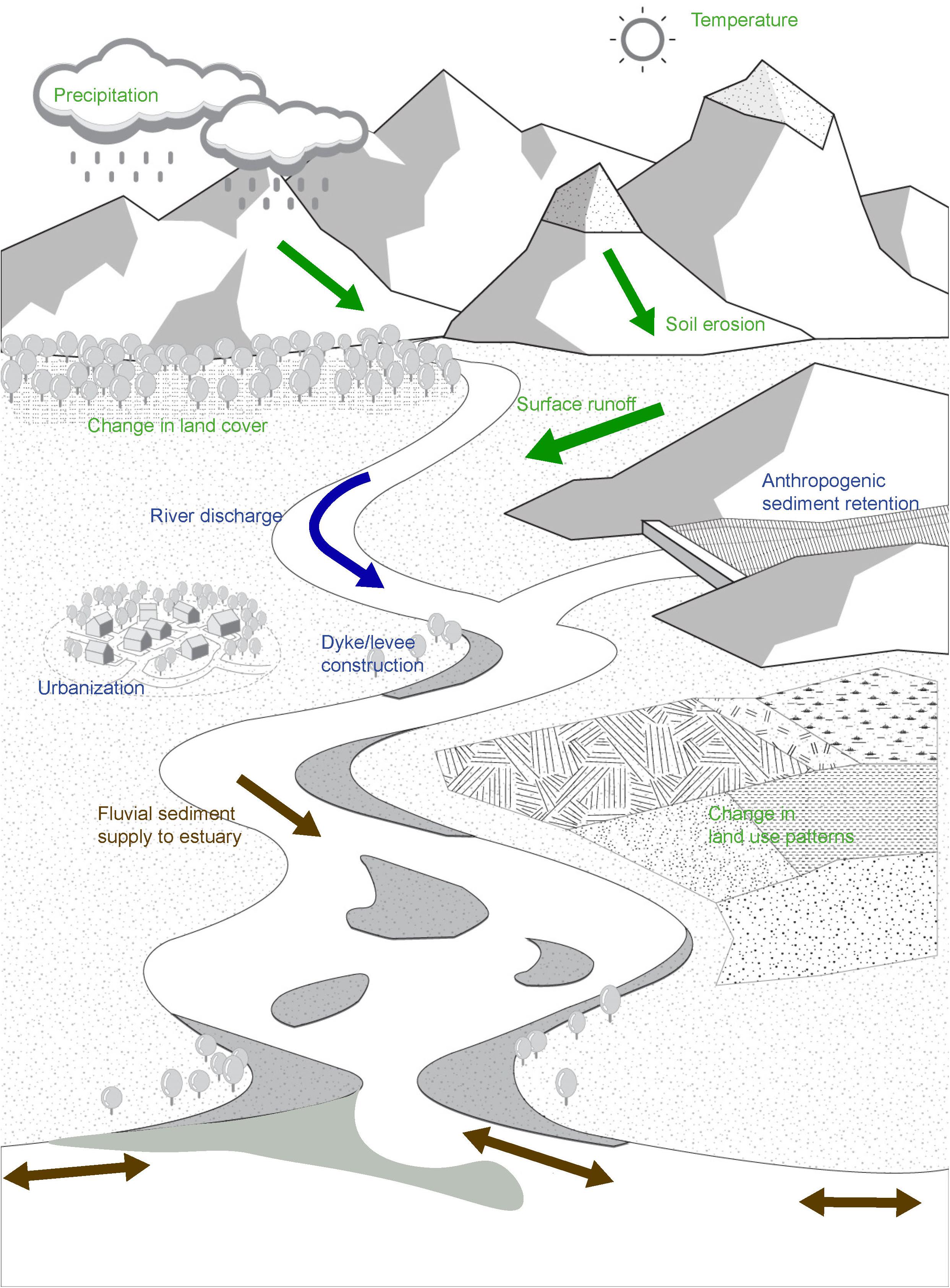
Figure 1. Schematic representation of the sediment pathway from source to the coast. The three colors used in the figure denote the major components (i.e., zones) related to this sediment pathway: (1) catchment-scale sediment production zone fed by soil erosion (in green), (2) transition zone of sediment throughput (in blue), and (3) deposition and redistribution zone dominated by sediment exchange between the estuary and its adjacent coast (in brown). Two-way arrows in brown denote sediment exchange between the estuary and its adjacent inlet-interrupted coast.

Globally, rivers contribute about 95% of the sediment received by the oceans (Syvitski et al., 2003). Generation of this sediment starts in the mountains, where rocks weather into sediment through mechanical, chemical and biological processes (Syvitski and Milliman, 2007). Climate change is expected to result in increased temperatures (Stocker et al., 2013b), which will affect both chemical and mechanical weathering, thus increasing the rate of soil erosion at the catchment scale (Syvitski et al., 2003; Syvitski and Milliman, 2007). Future changes in precipitation will also affect the amount of soil eroded at catchment scale. The rate of sediment generation at catchment scale also depends on anthropogenic activities, such as land clearance for agriculture, urbanization, road construction and de-and re-forestation (Syvitski and Milliman, 2007; Syvitski et al., 2009; Overeem et al., 2013). All these climate-change impacts and anthropogenic activities will alter the magnitude of sediment production at catchment scale, which, in turn, will affect the sediment volume received by the coast.

Sediment generated in the catchment is transported to the coast by rivers. Climate-change driven variations in future precipitation will alter the river discharge, thus affecting the throughput of eroded soil material at catchment scale (Syvitski et al., 2003; Kettner et al., 2005; Shrestha et al., 2013). Anthropogenic activities, however, will exert significant influences on the ultimate fluvial sediment supply to the coast. Activities that reduce the fluvial sediment supply capacity include anthropogenic sediment retention by dams, river sand mining, reduction in sedimentation area due to levee/dyke construction, and reduction in river flow due to water withdrawal for irrigation/drinking water supply. On the other hand, activities such as increased surface runoff due to urbanization and deforestation would increase the fluvial sediment loads (Verstraeten and Poesen, 2001; Vörösmarty et al., 2003; Syvitski, 2005; Syvitski and Milliman, 2007; Syvitski and Saito, 2007; Slagel and Griggs, 2008; Syvitski et al., 2009; Walling, 2009; Overeem et al., 2013; Chu, 2014; Ranasinghe et al., 2019). In combination, these anthropogenic activities and climate-change driven impacts can change the total fluvial sediment throughput from the catchment to the coast.

The final segment of the sediment pathway from catchment to the coast is the deposition and redistribution of sediment within the estuary and the adjacent inlet-interrupted coast. The estuarine accommodation volume is affected by both the sediment input from the river and anthropogenic influences within the estuary, such as sand mining, construction of causeways, bridges, and finger canals (Davis and Barnard, 2000; Barnard and Kvitek, 2010; Dallas and Barnard, 2011). Climate-change induced sea-level rise will increase the accommodation space within the estuary. The net sediment volume imported or exported by the estuary is, therefore, a direct function of the relative magnitudes of the sediment demand from the increased accommodation space, fluvial sediment supply, and the anthropogenic activities within the estuary. Depending on whether the estuary is a sediment importing or exporting system, the inlet-interrupted coast may, respectively, recede or prograde (Ranasinghe et al., 2013; Ranasinghe, 2016). The spatio-temporal alongshore variation of the coastline recession/progradation is a function of the relationship between the sediment volume exchange between the estuary and the adjacent coast and wave driven longshore sediment transport capacity in the vicinity of the inlet (Dalrymple, 1992; Dalrymple and Choi, 2003, 2007).

Due to the complex interplay and dependencies between coastline change and catchment, estuarine and coastal processes, any modeling technique that attempts to simulate long-term evolution of inlet interrupted coasts would benefit by considering the holistic behavior of Catchment-Estuary-Coastal (CEC) systems. However, only a limited number of studies to date have considered these systems in a holistic way (e.g., Shennan et al., 2003; Samaras and Koutitas, 2012; Ranasinghe et al., 2013). To investigate the interactions between the subsystems (catchment/fluvial, estuarine, and coastal), a range of modeling approaches are theoretically possible. In one end member, for each subsystem, models representing the relevant processes in as much detail as possible, resolving time and space scales as finely as possible, could be coupled together. Highly detailed models are available for some of the processes in some of the subsystems. For example, models representing flow and sediment transport on time and space scales that allow explicit simulation of hydrodynamics (based directly on approximations to the Navier Stokes equations) could theoretically be employed to represent fluvial, estuarine and coastal morphodynamics. Although the term “process-based” has often been used to describe such highly detailed models currently being used in practice (e.g., Delft3D, Mike21). Since a wide range of modeling approaches are in fact used to simulate physical processes, whether represented on the finest scales practical or on larger scales, here we avoid using the term “process based” and use the more generic term “highly detailed” instead.

There are three obstacles to coupling together an array of highly detailed models in the context of this study. First, processes in the subsystems involve physical, ecological, and human dynamics-and their couplings, but highly detailed models are not available for all of the relevant dynamics and couplings. Second, even when based on state-of-the-art representations of small-scale processes and parameterizations for sub-grid processes, highly detailed models, like all models, are imperfect. Model imperfections can cascade up through the scales when explicitly representing dynamics on scales much smaller than those of interest, especially where long-term simulations are concerned, limiting the quantitative reliability of model results on the scales of interest (Murray, 2007). Finally, limits on computational power make the use of a highly detailed modeling approach to simulate holistic behavior of CEC systems at 50–100 year time scales a daunting task. Therefore, presently available highly detailed modeling approaches are not capable of providing the probabilistic estimates of coastline change via multiple model realizations, which are needed by coastal zone planners/managers for risk-informed decision making (Ranasinghe, 2016, 2020).

To holistically model CEC systems, here we use an approach which represents the aggregated effects that processes occurring on much smaller scales have on the scales of interest, rather than explicitly resolving the interactions between myriad degrees of freedom that can be identified on much smaller scales. This approach embraces the way modeling (conceptual, analytical and numerical) has most often been done in Earth-surface science (Murray, 2013). For example, when simulating interactions on a macroscopic scale, e.g., hydrodynamics, we use parameterizations representing the collective effects at macroscopic scales of interactions between the many degrees of freedom that appear at microscales. For example, the Navier Stokes equations are in a sense parameterizations describing the interactions between macroscopic variables (e.g., pressure, density) that emerge from the collective dynamics at microscales (e.g., molecular dynamics). Thus, the modeling approach adopted here might best be termed “Appropriate Complexity” (French et al., 2016), since it embraces the philosophy of representing processes and interactions at scales commensurate with those of the phenomena of interest to effectively address dynamics at that scale. In this sense, models resolving hydrodynamic and sediment dynamics on fine time and space scales have an appropriate level of complexity for addressing questions across a range of scales, but models that aggregate the effects of those detailed processes to address questions on much larger scales are also appropriate. Compared to more highly detailed models, models in Earth-surface science using a more synthesized (Paola, 2000) or scale-aggregated approach have often been called “Reduced Complexity” models. We recognize that this term has its drawbacks (French et al., 2016), including the fact that all models are “reduced complexity” compared to the natural (or anthropogenic) systems they are representing.

The Scale-aggregated Model for Inlet-interrupted Coasts (SMIC) presented by Ranasinghe et al. (2013) is the first of its kind that treats CEC systems holistically while giving due consideration to the description of physics governing the behavior of the integrated system. Although SMIC provides a platform to probe into CEC systems holistically, its utility to address the long-term evolution of inlet-interrupted coasts under climate change impacts and anthropogenic activities is limited by (a) its applicability to only small tidal inlets, (b) its simplistic method of quantifying the fluvial sediment supply, and (c) the omission of alongshore spatio-temporal variation in coastline change. The present study attempts to address these shortcomings by developing a more generally applicable modeling tool that can simulate the climate-change driven evolution of inlet-interrupted coasts at macro (50–100 year) time scales.

It should be noted that the model developed here is partly data driven, using empirically-based parameterizations representing the behaviors of some component subsystems (e.g., terrestrial sediment yield). Representing the emergent effects of much smaller scale processes with empirically-based parameterizations can potentially be more quantitatively reliable than basing a model explicitly on the smaller scale dynamics (even if computational power were not a limitation), avoiding the possible cascade of model imperfections (Murray, 2007).

It is important to note that inlet-interrupted coasts include both mainland and barrier island coasts. For inlet-interrupted coasts along the mainland, sediment deposition and redistribution processes are closely linked with the type of estuary they are attached to (Ranasinghe et al., 2013; FitzGerald et al., 2014). The scope of this study is restricted to the long-term evolution of inlet-interrupted coastlines attached to bar-built (barrier) estuaries, which are commonly found along mainland sandy coasts located in wave-dominated, micro-tidal environments. Examples of bar-built estuaries can be seen along the eastern coast of the United States (near mid-latitudes), the Gulf of Mexico, Australia, Brazil, India, and in the regions of Amazon and Nile River (Ranasinghe et al., 1999; Davis and Fitzgerald, 2003; Woodroffe, 2003).

This study concentrates on coastlines interrupted by (a) estuaries with low-lying margins, and (b) small tidal inlets. Estuaries with low-lying margins contain tidal flats and salt marshes along their margins as well as banks with mild slopes. In these systems, increased sea level would lead to a significant increase in surface area of the estuary surrounded by mildly sloping banks, leading to an increase in the tidal prism, and consequently affecting the inlet cross-section area (O’Brien, 1969). On the other hand, small tidal inlets can be considered as a unique subset of barrier estuaries that (generally) have little or no intertidal flats, tidal marshes or ebb-tidal deltas (Duong et al., 2016, 2017, 2018).

Materials and Methods

Part of the future coastline change at tidal inlets will arise from changes in the net volume of sediment exchanged between inlet-estuary systems and their adjacent coast (Stive et al., 1998; Stive and Wang, 2003), driven by climate change and anthropogenic activities. This exchange sediment volume can be discretized into three main components: (1) basin (or estuary) infilling volume due to the sea level rise-induced increase in accommodation space, (2) basin (or estuary) volume change due to variation in river discharge, and (3) change in net annual fluvial sediment supply (Ranasinghe et al., 2013). Depending on whether the estuary is in sediment importing or exporting mode (relative to the ocean side of the estuary), and the magnitude of the aforementioned three sediment budget components, an inlet-affected coastline will experience a certain amount of coastline recession or progradation. In addition, the entire coastal profile is expected to respond to sea-level rise by moving landward and upward (Bruun, 1962); a process now commonly referred to as the Bruun effect. The model developed in this study mainly revolves around the physics-based representation of these processes and the way they interact with each other in driving coastline change.

Change in Total Sediment Volume Exchange Between a Barrier-Estuary System and Its Inlet-Interrupted Coast

Assuming the system is presently in dynamic equilibrium, the first step in determining the evolution of an inlet-interrupted coastline is to compute the change in the net annual volume of sediment exchanged between the inlet-estuary system and its adjacent coast. This calculation presumes that any given inlet-estuary system would tend toward and eventually reach its natural equilibrium. Hence, any excess amount of sediment would be exported to its adjacent coast. If there is a deficit in sediment (from the equilibrium value), an inlet-estuary system will import sand from its adjacent coast. This sediment volume can be computed by the summation of the three different processes mentioned above, and given by the following equation (Ranasinghe et al., 2013):

$$\mathrm{\Delta }{V}_{\text{T}}=\mathrm{\Delta }{V}_{\text{BI}}+\mathrm{\Delta }{V}_{\text{BV}}+\mathrm{\Delta }{V}_{\text{FS}}(1)$$

where ΔV_T is the cumulative change in the total sediment-volume exchange between the estuary and its adjacent coast, ΔV_BI is the sediment demand of the basin due to sea-level rise-driven change in basin volume (i.e., basin infilling volume), ΔV_BV is the change in basin infill sediment volume due to variation in river discharge, and ΔV_FS is the change in fluvial sediment supply due to combined effects of climate change and anthropogenic activities (all volumes in m³).

Sea-level rise may affect the tides as well. However, possible changes in tides due to rising sea level are projected to be marginal. For example, Pickering et al. (2017) have shown that for 2.0 m of sea-level rise, the possible changes in the mean high water level of tides are less than 0.1 m. Therefore, this aspect was not considered in this study. Further, the nodal tidal elevation changes (e.g., Baart et al., 2012; Peng et al., 2019) are also not taken into account in the present model.

The schematic diagram presented below (Figure 2) shows the connectivity among these processes and the sediment-volume components comprising ΔV_T.

FIGURE 2

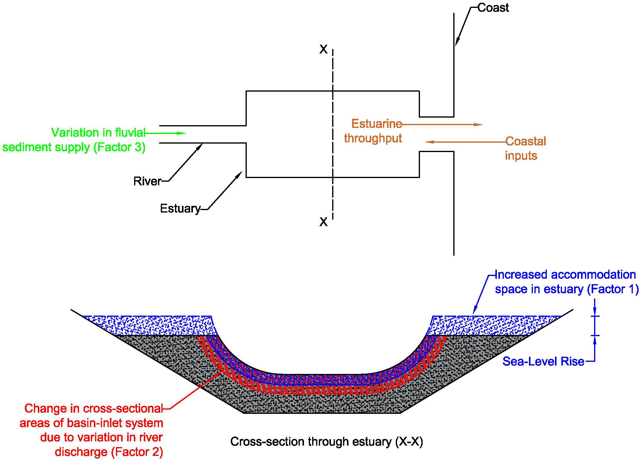
Figure 2. Schematic illustration of the connections between sediment volume components associated with the change in total sediment-volume exchange (ΔV_T) between inlet-estuary system and its adjacent coast.

Basin Infilling Volume Due to Sea-Level Rise-Induced Increase in Accommodation Space

Accommodation space is the additional volume created within the basin (or estuary) due to an increase relative mean sea level [ΔRSL (m)]. This increase in volume, given by A_b.ΔRSL; where, A_b is the basin surface area (m²), results in an extra sediment demand by the estuary [ΔV_BI (m³); Factor 1 in Figure 2]. Taking into account also the time lag between sea-level rise (hydrodynamic forcing) and the associated basin infilling (morphological response), ΔV_BI can be expressed by the following equation, where the negative sign indicates sediment imported into the inlet-estuary system.

$$\mathrm{\Delta }{V}_{\text{BI}}=-\text{fac}\left(A_{\text{b}}\mathrm{\Delta }RSL\right)(2)$$

where “fac” (0 < fac < 1) accounts for the morphological response lag. In this study, it is taken as 0.5 (following the argumentation and formulations in Ranasinghe et al. (2013) for the original SMIC model) in all model simulations.

Basin Volume Change Due to Variations in River Flow

Changes in river discharge [ΔQ_R (m³)] will affect the infill volume of the estuary. Such changes in river discharge would alter the tidal flow volume during the ebbing phase of the tide, and subsequently, the estuarine and inlet velocities. Due to the tendency of velocities in a basin-inlet system (averaged over the net cross section) to approach an equilibrium value, the basin-inlet system will change its cross-section by either scouring or accretion, until the equilibrium cross section is reached. Depending on the sign of change in future river discharge [i.e., increase (+)/decrease (−)], a particular volume of sediment [ΔV_BV(m³); Factor 2 in Figure 2] would be exchanged between the inlet-basin system and its adjacent coast to accommodate this basin-inlet cross-sectional change. This sediment volume (ΔV_BV) can be computed as follows (Ranasinghe et al., 2013):

$$\mathrm{\Delta }{V}_{\text{BV}}=\frac{\mathrm{\Delta }{Q}_{\text{R}}{V}_{\text{B}}}{\left(P+Q_{\text{R}}\right)}(3)$$

where Q_R is the present river flow into the basin during ebb (m³), ΔQ_R is the climate change-driven variation in river flow during ebb (m³), V_B is the present basin volume (m³), and P is the mean equilibrium ebb-tidal prism (m³).

Determining equilibrium tidal prism for estuaries with low-lying margins

The above sediment volume ΔV_BV depends on the equilibrium tidal prism. This equilibrium tidal prism in estuaries with low-lying margins is linked with the concurrent sea level and cross-sectional area of the tidal inlet and channels in the basin. When the sea level is gradually increasing, as it is doing now (Stocker et al., 2013b), it is necessary to determine the equilibrium tidal prism at these inlet-estuary systems for the increased mean sea level, so that the corresponding basin volume change and subsequent amount of sediment exchange can be correctly computed. Figure 3 illustrates the non-linear, iterative calculation procedure adopted here to represent this phenomenon, followed by a description of the associated physical processes.

FIGURE 3

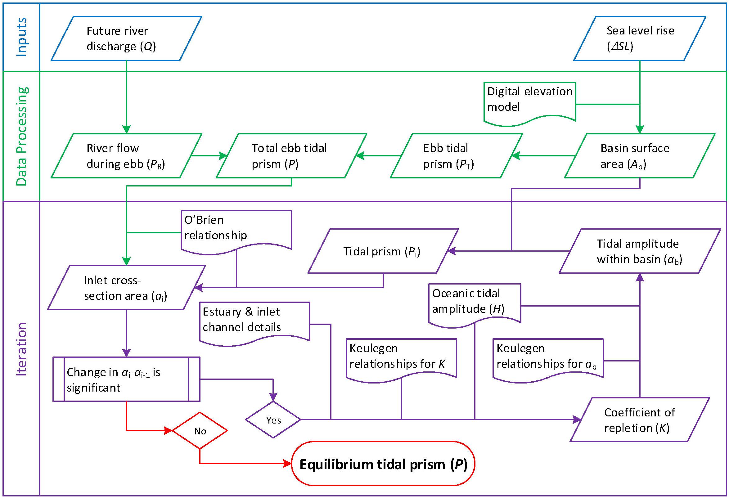
Figure 3. Flowchart of the iteration procedure to determine equilibrium tidal prism at estuaries with low-lying margins (modified from Bamunawala et al., 2018b).

The total ebb-tidal prism (P) consists of two components: (1) the volume of water flowing out of the estuary system due to tidal forcing alone (P_T), and (2) the volume of water supplied by the river flow during the ebbing phase of the tide (P_R).

$$P=P_{\text{T}}+P_{\text{R}}(4)$$

Owing to the low-lying margins of these systems, the basin surface area of the estuary (A_b) will change with sea-level rise. Therefore, a look-up table for the basin surface area was developed with the aid of a Digital Elevation Model (DEM), to determine the basin surface area (A_b) associated with different sea levels.

Assuming there is no phase lag in tidal elevations within the systems, which is a reasonable assumption for not-very-long estuaries (Dronkers, 1964) the ebb-tidal prism (P_T) corresponding to this new basin surface area can be calculated according to the relationship presented by Keulegan (1951).

$$P_{\text{T}}=A_{\text{b}}(2a_{\text{b}})(5)$$

where A_b is the surface area of the estuary and a_b is the mean tidal amplitude within the estuary.

Tidal inlets throughout the world exhibit several consistent relationships that have allowed coastal engineers and marine geologists to formulate predictive models. One such widely-known relationship is O’Brien’s relationship between inlet channel cross-sectional area (a) and tidal prism (P) (O’Brien, 1969).

$$a=c_1{P}^{c_2}(6)$$

where c₁ and c₂ are empirical coefficients.

It should be noted that there can be instances where the estuary systems deviate from the above a-P relationship (e.g., Hume and Herdendorf, 1993; Gao and Collins, 1994). Townend (2005) suggested that the deviation from the a-P relationship can be attributed to the state of the respective estuary system’s response to contemporary processes over the Holocene. Besides, there are some other systems, of which the geological constraints do not accommodate the eroding of the inlet channel. In such cases, the tidal prism has to change to maintain the equilibrium conditions.

Thus, when P changes, the inlet cross-sectional area a will also need to change. According to Keulegan (1951), such changes in the inlet cross-sectional area could also affect tidal attenuation characteristics in the inlet channel as attenuation is a function of the inlet-channel geometry. Table 2 of Keulegan (1951) provides a look-up table for an expression (left-hand side of the equation below), which includes the coefficient of repletion (K), basin surface area (A_b), inlet channel cross-sectional area (a) and oceanic tidal amplitude (H) for a given inlet-channel length (L_c), inlet-channel hydraulic radius (r) and Manning’s roughness (n).

$$\frac{A_{\text{b}}K\sqrt{H}}{a}\times {10}^{-4}=\text{f}(n,r,L_{\text{c}})(7)$$

This relationship allows determining the coefficient of repletion (K). The resulting tidal amplitude within the basin (a_b) can then be computed using:

$$\frac{a_{\text{b}}}{H}=\sin (\mathrm{\tau })(8)$$

where sin⁡(τ) is a function of the coefficient of repletion (K), and can be determined through another look-up table (Table 4) provided in Keulegan (1951).

It should be noted that Eqs 7 and 8 inherently assume that the presence of a narrow and relatively straight inlet channel which connects the ocean to an estuary/lagoon that is significantly wide compared to the inlet channel.

Use of the above computed tidal amplitude in Eq. (5) provides the new tidal prism (for the considered mean sea level), which will consequently result in a new inlet cross-sectional area as per Eq. (6). A new inlet cross-sectional area will have a different coefficient of repletion (K) and, thus a new tidal amplitude within the basin. Therefore, Eqs (5–8) are here used iteratively, until the difference between two subsequent computed inlet cross-sectional areas (for a given mean sea level) is less than 1% of the former value (Figure 3).

Change in Fluvial Sediment Supply

Climate change and anthropogenic activities could result in significant changes in the annual fluvial sediment volume [ΔQ_S (m³)] supplied to the coast (Vörösmarty et al., 2003; Syvitski, 2005; Palmer et al., 2008; Ranasinghe et al., 2019). Consequently, these changes will affect the total volume of sediment exchanged between the inlet-estuary system and its neighboring coast [ΔV_FS (m³); Factor 3 in Figure 2] over the period considered [t (in years)]. The changes in fluvial sediment volume are here calculated as (Ranasinghe et al., 2013):

$$\mathrm{\Delta }{V}_{\text{FS}}=\underset{0}{\overset{t}{\int }}\mathrm{\Delta }{Q}_{\text{S}}(t)\mathit{d}t(9)$$

Assessment of fluvial sediment supply to coasts

Sediment generation and fluvial sediment throughput at catchment scale are affected by both climate change-driven impacts and anthropogenic activities (Syvitski et al., 2003, 2009; Syvitski and Milliman, 2007; Shrestha et al., 2013). Bamunawala et al. (2018a) illustrated that the empirical BQART model presented by Syvitski and Milliman (2007) can be used effectively to assess the annual fluvial sediment supply to the coast while considering both climate change-driven impacts and human activities. This empirical model is based on 488 globally-distributed datasets. For catchments with a mean annual temperature greater than or equal to 2°C, the BQART model estimates the annual sediment volume (Q_S) transported downstream to the coast by the following equation:

$$Q_{\text{S}}=\mathrm{\omega }B{Q}^{0.31}{A}^{0.5}RT(10)$$

where ω is 0.02 or 0.0006 for the sediment volume (Q_S), expressed in kg/s or MT/year, respectively, Q is the annual river discharge from the catchment considered (km³/yr), A is the catchment area (km²), R is the relief of the catchment (km), and T is the catchment-wide mean annual temperature (°C).

Term “B” in the above equation represents the catchment sediment production and comprises glacial erosion (I), catchment lithology (L) that accounts for its soil type and erodibility, a reservoir trapping-efficiency factor (T_E), and human-induced erosion factor (E_h), which is expressed as the following equation:

$$B=IL(1-T_{\text{E}})E_{\text{h}}(11)$$

Glacial erosion (I) in the above equation is expressed as follows:

$$I=1+(0.09A_{\text{g}})(12)$$

where A_g is the percentage of ice cover of the catchment area.

Syvitski and Milliman (2007) stated that the human-induced erosion factor (E_h; anthropogenic factor) depends on land-use practices, socio-economic conditions and population density. In their study, E_h values were determined based on the Gross National Product (per capita) and population density. Based on the global dataset used, the optimum range of E_h was suggested to be 0.3–2.0.

In this study, however, instead of using coarse countrywide estimates of Gross National Product (GNP)/capita and population density to estimate the human-induced soil erosion factor (E_h), the human footprint index (HFPI), which is based on high-resolution spatial information published by the Wildlife Conservation Society [WCS] and Columbia University Center for International Earth Science Information Network [CIESIN] (2005) is used to achieve a better representation of anthropogenic influences on sedimentation (Balthazar et al., 2013; Bamunawala et al., 2018a). The HFPI is developed by using several global datasets such as population distribution, urban areas, roads, navigable rivers, electrical infrastructures and agricultural land use (Sanderson et al., 2002).

Reference Conditions for Baseline Simulations

The modeling approach presented above is used here to compute the total sediment exchange volume between the inlet-estuary system and its adjacent coastline for the 2020–2100 period. In order to compute these future changes, first, baseline conditions need to be established. Here, CEC system conditions at 2019 were used as the reference condition in all sediment-volume computations. However, as both mean annual temperature (T) and cumulative river discharge (Q) show significant inter-annual variability, using T and Q values specifically for the year 2019 as the reference condition would not be accurate. Therefore, the mean values of T and Q over the last decade (2010–2019) were used as the reference conditions for these two variables. As there is no significant inter-annual variability in mean sea level, all future changes in sea level over the 2020–2100 period were computed relative to the 2019 mean sea level.

Modeling the Spatio-Temporal Evolution of Inlet-Interrupted Coastlines

Changes in the total sediment exchange between barrier estuaries and their adjacent coasts (ΔV_T) will act as sediment source/sink at the coast, which, in turn, will contribute to the evolution of the inlet-interrupted coast. The extent and magnitude of such coastline variations are also related to the wave-driven longshore sediment transport capacity in the vicinity of the inlet. Many studies have indicated that potential climate-change impacts during the 21^st century may result in changing mean wave conditions across the world’s oceans (Mori et al., 2010; Hemer et al., 2013; Semedo et al., 2013; Casas-Prat et al., 2018; Morim et al., 2019). Such changes in wave conditions could result in variations in longshore sediment transport rates and gradients therein (e.g., Hemer et al., 2012; Casas-Prat and Sierra, 2013; Erikson et al., 2015; Grabemann et al., 2015; Wolf et al., 2015; Dastgheib et al., 2016; Shimura et al., 2016). However, all available wave projections only provide averaged changes of wave conditions [i.e., not for individual Representative Concentration Pathways (RCPs)] over the last two/three decades of the 21^st century (i.e., not for the entire 21^st century). Furthermore, projected changes in offshore wave conditions are rather small for most of the global coastline, especially where sandy coasts are concerned, implying that associated changes in nearshore waves would also be small. Therefore, in this study, which considers all RCPs over the entire 21^st century, it is assumed that the ambient rates of longshore sediment transport remain invariant throughout the 21^st century, and thus, the projected changes in coastlines are computed based on the present-day longshore sediment transport rates. With this assumption, the conceptual framework used to compute the spatio-temporal variations of inlet-interrupted coastlines is described below.

Following the overarching objective of this study, a simplified framework of a generically applicable coastline model that provides first-order estimates of coastline variations at macro time scales was developed. It represents the general changes of the inlet-interrupted coastline by considering the total change in sediment volume exchange between the inlet-estuary system and the adjacent coast (ΔV_T), while assuming uniform shoreline orientations along up- and down-drift coasts and the lack of any coastal structures.

The maximum extent of inlet-affected coastline in both up-drift and down-drift directions from an inlet is constrained by the existence of headlands, rock outcrops, inlets or by other prominent changes in mean shoreline orientation. Following the method adopted in the SMIC applications by Ranasinghe et al. (2013), the maximum extent of this inlet-affected coastline distance was considered to be ∼25 km. If there is no known gradient in the net annual alongshore sediment transport rate along the coastline (i.e., both up- and down-drift coasts), it can be assumed that the coastal cell concerned is presently in equilibrium at annual time scales.

Within the development of this simplified coastline change model, it is assumed that the longshore sediment transport (LST) occurs uniformly over the cross-shore profile. Figure 4 illustrates the hypothetical equilibrium cross-shore profile. Given that the change in total sediment volume exchange (ΔV_T) is computed annually (Eqs 1–12), ΔV_T is first divided into a number of equal fragments (n_v). This volume fragment (V_fr), which is calculated using Eq. [13] was then distributed along the coastline.

FIGURE 4

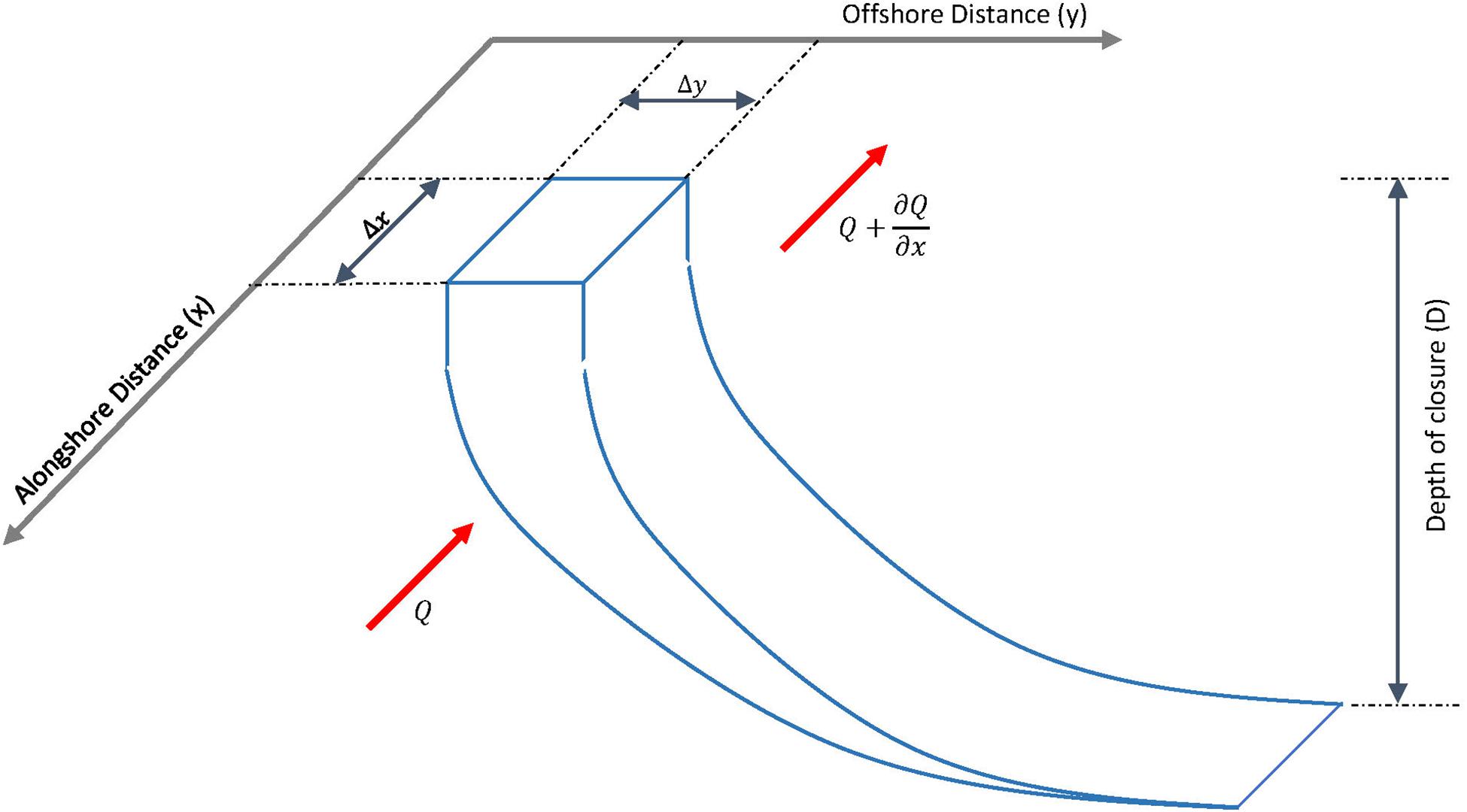
Figure 4. Schematic illustration of a hypothetical equilibrium cross-shore profile and the variables used in developing the one-line coastline change model.

$$V_{\text{fr}}=\frac{\mathrm{\Delta }{V}_{\text{T}}}{n_{\text{v}}}(13)$$

Depending on the equivalent longshore transport capacity (ΔQ_LST; calculated using Eq. 14), all or part of this volume fragment is transported along the coast.

$$\mathrm{\Delta }{Q}_{\text{LST}}=\frac{Q_{\text{LST}}}{n_{\text{v}}}(14)$$

Following the assumption of a balanced sediment budget within the coastal cell, any volume of sediment that gets transported in the down-drift direction will result in coastal progradation at the farthermost section of the down-drift coast. If the volume fragment is larger than the equivalent longshore transport capacity (ΔQ_LST), the surplus volume (ΔV; computed using Eq. 15) will result in a seaward translation of the coastline position (Δy) within the considered alongshore distance (Δx) (Figure 4). This also holds when V_fr < ΔQ_LST, which will lead to coastline recession.

$$\mathrm{\Delta }V=V_{\text{fr}}-\mathrm{\Delta }{Q}_{\text{LST}}(15)$$

Assuming that the shoreline moves cross-shore parallel to itself while maintaining its equilibrium profile, the following relationship can be derived to determine the resulting change in coastline position (Δy).

$$\text{min}(\mathrm{\Delta }V,V_{\text{fr}})=\mathrm{\Delta }x(D\mathrm{\Delta }y)$$

where D is the depth of closure.

The above procedure is repeated n_V times, so that the total change in sediment volume exchange between the estuary and adjacent coast (ΔV_T) is fully distributed along the coastal cell. These computations are closely connected to an expression for the longshore sediment transport rate (Q_LST), which, in turn, is related to the longshore current generated by oblique incident breaking waves. Q_LST is thus presented as:

$$Q_{\text{LST}}=Q_0\sin (2{\mathrm{\alpha }}_{\text{b}})(16)$$

where Q₀ is the amplitude of the longshore sediment transport rate (m³/yr), and α_b is the breaking wave angle between wave crest line and coastline, which can be expressed as follows, assuming small-angles:

$${\mathrm{\alpha }}_{\text{b}}={\mathrm{\alpha }}_0-\frac{\mathrm{\Delta }y}{\mathrm{\Delta }x}(17)$$

where α₀ (rad) is the angle of breaking wave crests (relative to the coastline).

Since the local coastline position (Δy) would be updated with the alongshore distribution of each volume fragment, breaking wave angle (α_b) and longshore sediment transport rate (Q_LST) are also updated after completion of the distribution of each volume fragment. If the present-day longshore sediment transport rate and the corresponding angle of breaking wave crest (α₀) are known, the above-described procedure can be implemented to distribute the sediment volume along the inlet-interrupted coast. If such information is not available, the amplitude of the longshore sediment transport rate (Q₀) can be reasonably estimated by using a bulk longshore sediment transport equation such as the CERC formula (CERC, 1984), the Kamphuis formula (Kamphuis, 1991), and the Bayram formula (Bayram et al., 2007). An example of such formulation of Q₀ [from the US Army corps, Coastal Engineering Research Centre (CERC), published in the Shore Protection Manual (CERC, 1984)] is shown in Eq. (18).

$$Q_0=\frac{0.77\sqrt{\text{g}}}{32(1-p)\left(\frac{{\mathrm{\rho }}_{\text{s}}}{\mathrm{\rho }}-1\right)\sqrt{{\mathrm{\gamma }}_b}}\times H_{\text{sb}}^{2.5}(18)$$

where H_sb is the significant wave height at breaker line (m), γ_b is the breaking parameter for irregular waves (0.55), ρ_s is the density of sand (2,650kg/m³), ρ is the density of seawater (1,030kg/m³), p is the porosity of sand (0.4), and g is the gravitational acceleration (9.81 m/s²).

In addition to the above-described coastline change, regional relative sea-level rise (ΔRSL) will shift the active cross-shore profile upward and landward, which, in the absence of sediment sources supplying sand to the coast, will result in additional coastline recession (Bruun, 1962). The magnitude of this so-called Bruun effect driven coastline recession is expressed according to the following equation:

$$\mathrm{\Delta }{C}_{\text{BE}}=\frac{\mathrm{\Delta }RSL}{\tan \left(\beta \right)}(19)$$

where ΔC_BE is the coastline recession (m), ΔRSL is the sea-level rise (m), and β is the average slope of the active beach profile from the shoreline to the depth of closure (D; Figure 4). It is important to note the the coastline change computed in this way will represent only the change that would be due to climate change impacts and will not be inclusive of any ambient coastline change that would occur even without any future variations in system forcing (e.g., due to alongshore gradients in LST, cross-shore feeding of sediment, fluvial sediment supply).

Input Data Sources

The reduced-complexity model presented in sections “Change in Total Sediment Volume Exchange Between a Barrier-Estuary System and Its Inlet-Interrupted Coast” and “Modeling the Spatio-Temporal Evolution of Inlet-Interrupted Coastlines,” requires four main drivers to project the long-term evolution of inlet-interrupted coasts: annual mean temperature (T), annual cumulative river discharge (Q), change in regional relative sea-level (ΔRSL), and anthropogenic activities in the catchment, as represented by the human-induced erosion factor (E_h).

Temperature and runoff projections were obtained from General Circulation Models (GCMs) of the Coupled Model Intercomparison Project Phase 5 [CMIP5 data portal; Earth System Grid-Centre for Enabling Technologies (ESG-CET); available on the webpage http://pcmdi9.llnl.gov/]. Projected daily/monthly values of temperature and surface runoff were obtained for all four Representative Concentration Pathways (RCPs). Initially, the GCMs with both temperature and surface runoff projections for all RCPs over the 2010–2100 period were considered as data sources. Of these, GCMs with spatial resolution finer than 2.5° were selected to obtain the necessary climate inputs (T and Q). Where possible, the suitability of the above-selected data sources was assessed regionally, by considering the guidelines published on the appropriateness of GCMs in respective areas (e.g., CSIRO and Bureau of Meteorology, 2015, for Australia).

According to Nicholls et al. (2014), the regional relative sea-level changes (ΔRSL) can be calculated according to the following equation:

$$\mathrm{\Delta }RSL=\mathrm{\Delta }S{L}_{\text{G}}+\mathrm{\Delta }S{L}_{\text{RM}}+\mathrm{\Delta }S{L}_{\text{RG}}+\mathrm{\Delta }S{L}_{\text{VLM}}(20)$$

where ΔRSL is the change in relative sea level, ΔSL_G is the change in global mean sea level, ΔSL_RM is the regional variation in sea level from the global mean due to meteo-oceanographic factors, ΔSL_RG is the regional variation in sea level due to changes in the earth’s gravitational field, and ΔSL_VLM is the change in sea level due to vertical land movement (all values in meters).

The regional relative sea-level change projections by 2100 (ΔRSL) were obtained from Figure TS.23 of Stocker et al. (2013a), while the corresponding global mean sea level change (ΔSL_G) was obtained from Table SPM. 2 of Stocker et al. (2013b). The difference between those two sets of values provide the cumulative contribution of ΔSL_RM, ΔSL_RG, and partly ΔSL_VLM (excluding any local subsidence/rebound) for 2100. Those differences were linearly distributed from the year 2000 to obtain the yearly cumulative contribution of ΔSL_RM, ΔSL_RG, and ΔSL_VLM. Those linearly distributed values were then added to the yearly changes in global mean sea level (ΔSL_G), following the method presented by Mehvar et al. (2016), to obtain yearly projections of regional relative sea-level changes. The yearly changes in global mean sea level (ΔSL_G) are calculated following Nicholls et al. (2014) as:

$$\mathrm{\Delta }S{L}_{\text{G}}={\text{a}}_{1}t+{\text{a}}_2{t}^2(21)$$

where; ΔSL_G is the change in global sea level (m) since 2000, “t” is the number of years since 2000, a₁ is the trend in sea level change (m/yr), and a₂ is the change in the rate of sea-level change trend (m/yr²). The relevant coefficients were obtained from Mehvar et al. (2016).

The HFPI data were obtained from the WCS-CIESN database, which is available at a spatial resolution of 30 arc-seconds and is regionally normalized to account for the interaction between the natural environment and human influences (Sanderson et al., 2002). Global and continental-scale raster files of HFPI data are available at https://doi.org/10.7927/H4M61H5F.

Case Study Sites and Input Data

The above-introduced reduced-complexity model was applied at three selected systems representing (a) barrier estuaries with low-lying margins (Alsea estuary, Oregon, United States, and Dyfi estuary, Wales, United Kingdom) and (b) small tidal inlets (Kalutara inlet, Sri Lanka). Table 1 summarizes the key properties of these systems and Figure 5 shows the locations of the selected case study sites, their respective watershed areas and HFPI.

TABLE 1

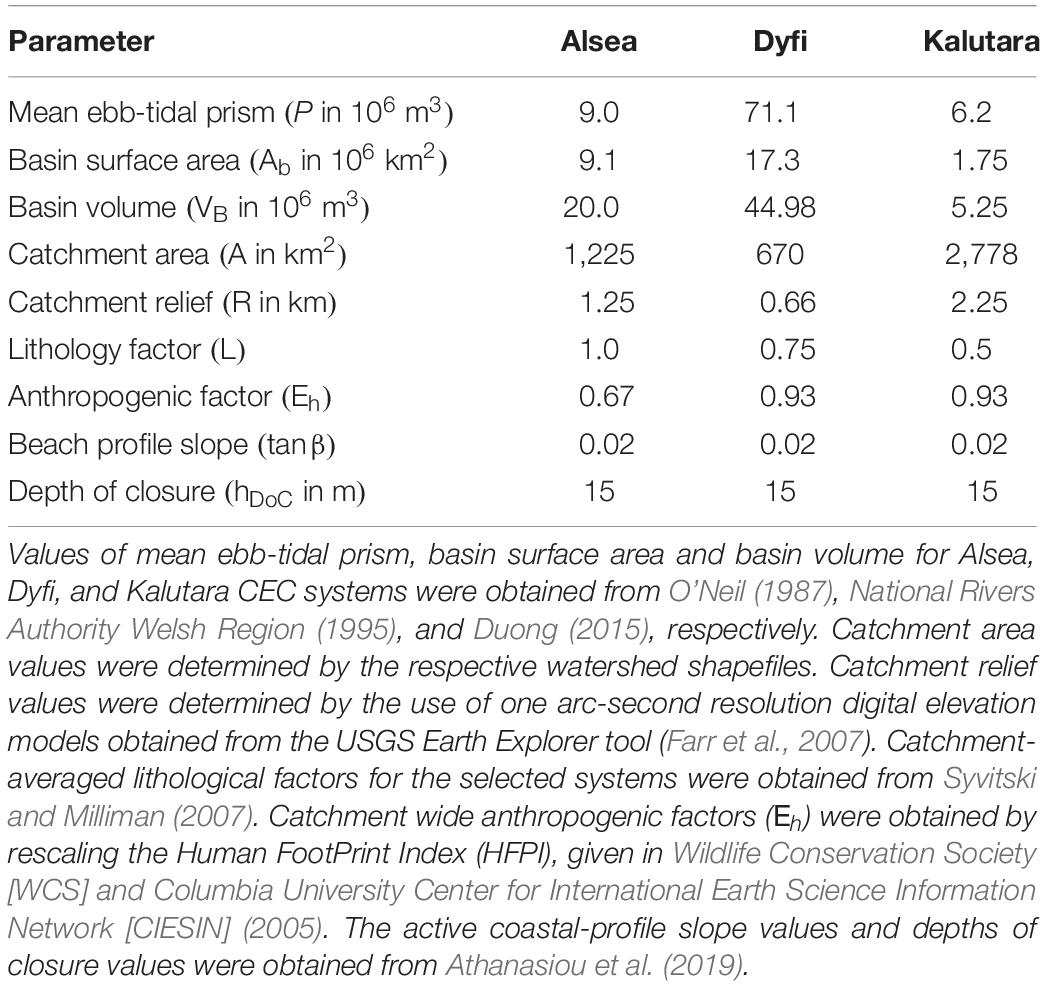
Table 1. Properties of the selected barrier estuary systems (reference conditions).

FIGURE 5

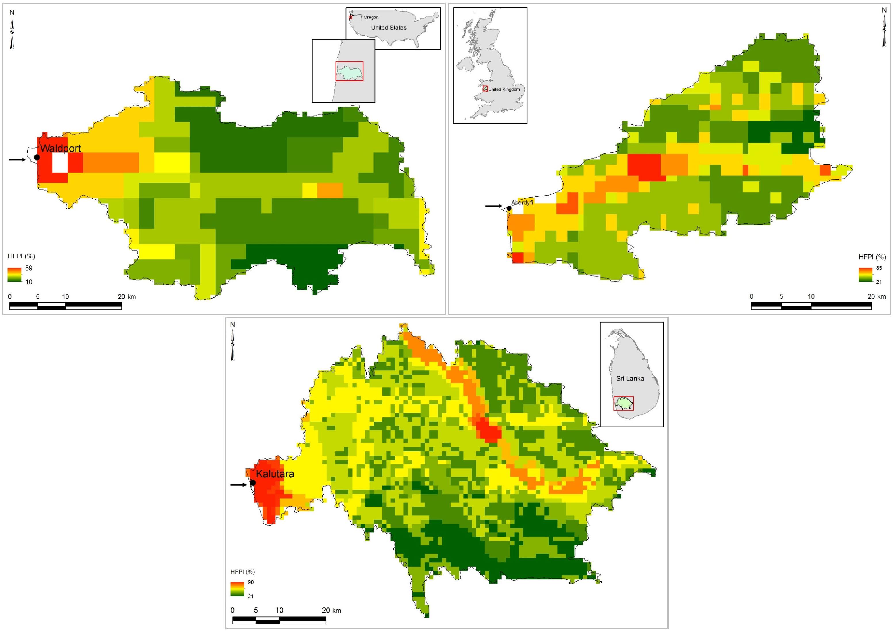
Figure 5. Human FootPrint Index (HFPI), location and watershed areas of the selected CEC systems (Alsea estuary: top-left, Dyfi estuary: top-right, and Kalutara estuary: bottom). HFPI data were obtained from https://doi.org/10.7927/H4M61H5F.

Present-day HFPI values within the catchment were rescaled linearly to fit the optimum scale of E_h suggested by Syvitski and Milliman (2007). These rescaled HFPI values were then averaged over the catchment to determine a representative factor for human-induced erosion (E_h). Given the contemporary rate of population growth and urbanization, it is safe to assume that E_h will increase by 2100. Owing to numerous uncertainties associated with such projections (e.g., Veerbeek, 2017), the value of E_h by 2100 was assumed to increase by 15% of its present-day value.

The T and Q values were obtained by an ensemble of four selected GCMs (viz., GFDL-CM3, GFDL-ESM2G, and GFDL-ESM2M from NOAA, United States, and IPSL-CM5A-MR from IPSL in France). Table 2 presents the averaged T and Q projections for the reference (2010–2019), mid-century (2046–2065), and end-century (2081–2100) periods, indicating the variation of the respective model inputs across the 21^st century for different RCPs.

TABLE 2

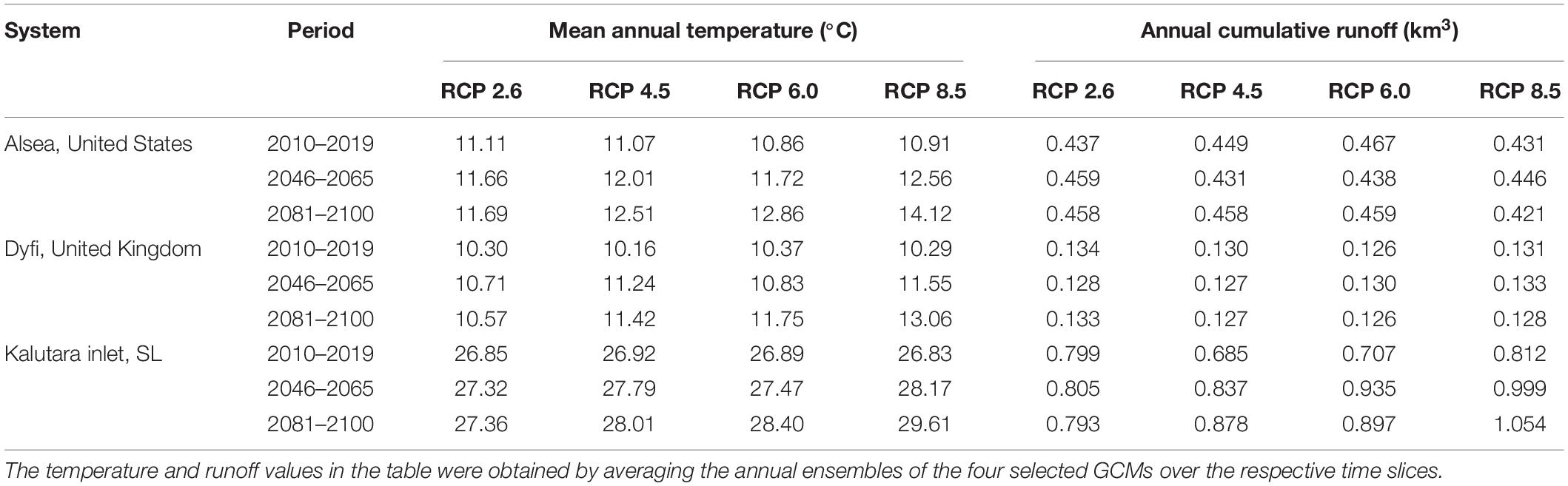
Table 2. Average annual mean temperature and cumulative runoff at the selected case study locations over the present, mid-21^st century and end 21^st century time slices.

Figure 6 shows the projected variations of regional relative sea-level (ΔRSL) at the selected study locations for the four RCPs.

FIGURE 6

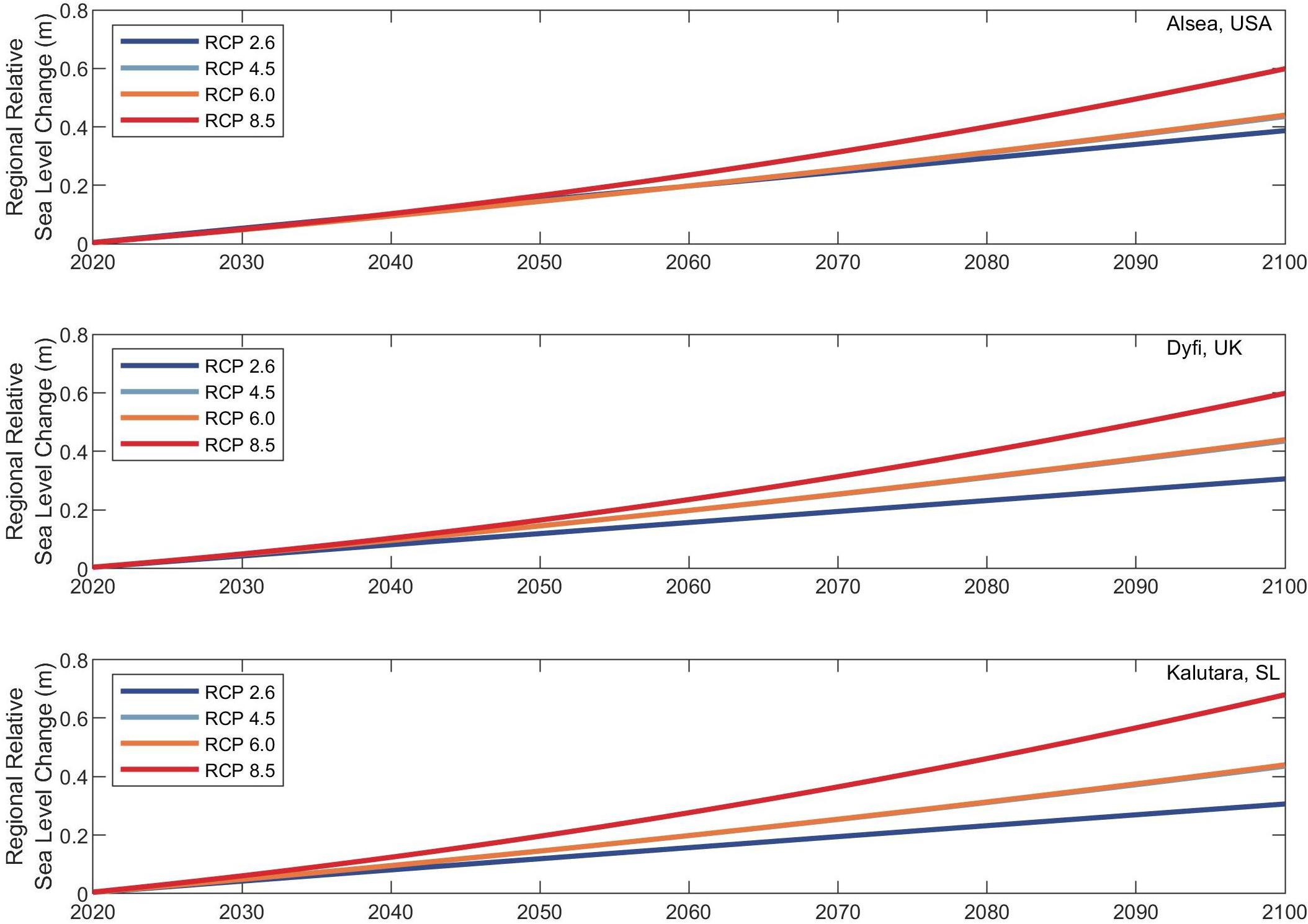
Figure 6. Projected regional relative sea level at the selected barrier-estuary systems for different RCPs. The top, middle, and bottom sub-plots are corresponding to Alsea, Dyfi, and Kalutara inlets, respectively. Different colors indicate the four RCPs (see legend insert in each sub plot).

Results

Model hindcasted coastline changes are presented in section “Model Hindcasts for the 1986–2005 Period.” Results of model applications at the three case study locations are presented in sections “Projected Variation of Total Sediment Volume Exchange (ΔV_T): 2020–2100” and “Projected Coastline Change at the Case Study Locations: 2020–2100.” Section “Projected Variation of Total Sediment Volume Exchange (ΔV_T): 2020–2100” presents, for each system, the projected variations in the total sediment volume exchange between the estuary and the adjacent coast (ΔV_T), together with an assessment of the predominant sediment volume component at each case study location. Section “Projected Coastline Change at the Case Study Locations: 2020–2100” presents the projected changes in coastline position at each location by 2060 and 2100.

Model Hindcasts for the 1986–2005 Period

As a model validation exercise, the above-presented modeling technique was applied to a historical period (1986–2005) to compare the model hindcasts with observed shoreline change at the studied mainland barrier estuary systems. To achieve this objective, the following simplifications were made when obtaining the model inputs/reference conditions.

For the historical period (1986–2005), the ensemble of GCMs described in section “Case Study Sites and Input Data” was used to obtain the yearly values of T and Q. The reference conditions for the T and Q for this hindcast period were taken as the mean value of the GCM ensemble over the 1976–1985 period. The rate of global mean sea-level rise was taken as 2.1 mm/yr for the 1986–2005 period, following the projections presented in Chapter 4 of the IPCC Special Report on the Ocean and Cryosphere in a Changing Climate (i.e., Oppenheimer et al., 2019). The present value of HFPI was considered as a constant throughout the historical period. The model hindcasted coastline changes at the three case study locations were compared with satellite-image based shoreline change rates presented by Luijendijk et al. (2018).

The results of the comparison are shown in Table 3. This comparison indicates that the modeled coastline change at all three systems for the validation period compare well with those observed over the same period, providing confidence in the model.

TABLE 3

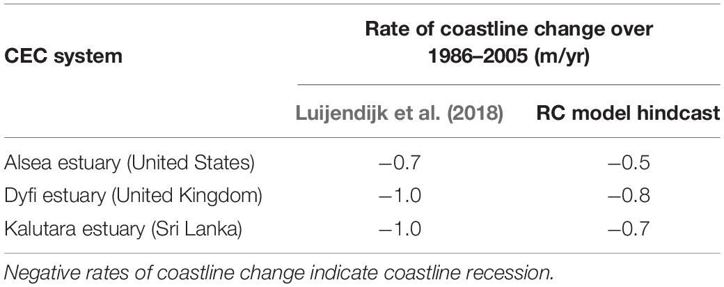
Table 3. Comparison of the model hindcasted rates of coastline change over 1986–2005 with the observed rates of coastline change obtained from Luijendijk et al. (2018).

Projected Variation of Total Sediment Volume Exchange (ΔV_T): 2020–2100

Figures 7–9 show the projected change in total sediment volume exchange (ΔV_T) between each case study estuary and the adjacent coast over the 21^st century (left) and the individual contributions of the three main sediment volume components [i.e., basin infilling (ΔV_BI), basin volume change (ΔV_BV), and fluvial sedimentation (ΔV_FS)].

FIGURE 7

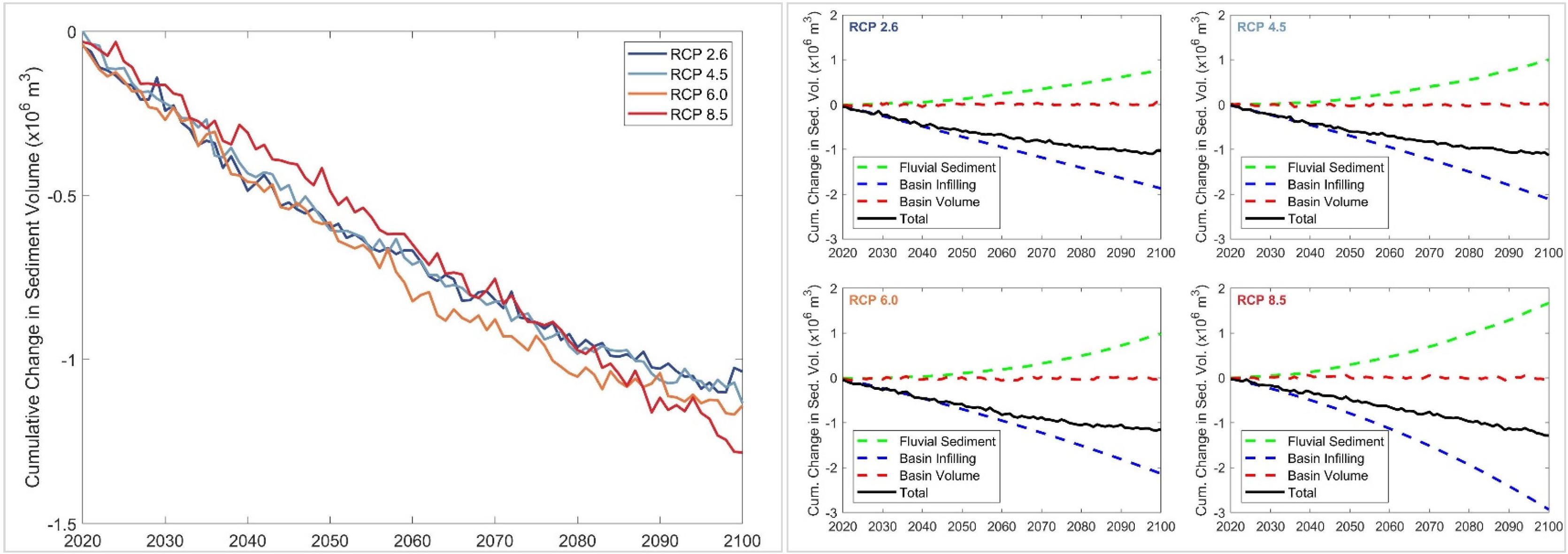
Figure 7. Projected change in total sediment volume exchange (ΔV_T) between the Alsea estuary and the adjacent coast (left), and the relative contributions of the three different sediment volume components (right) over the 21^st century for RCP 2.6, 4.5, 6.0, and 8.5. Negative and positive values of ΔV_T indicate sediment imported to the estuary from the adjacent coast and sediment exported from the estuary to the adjacent coast, respectively.

FIGURE 8

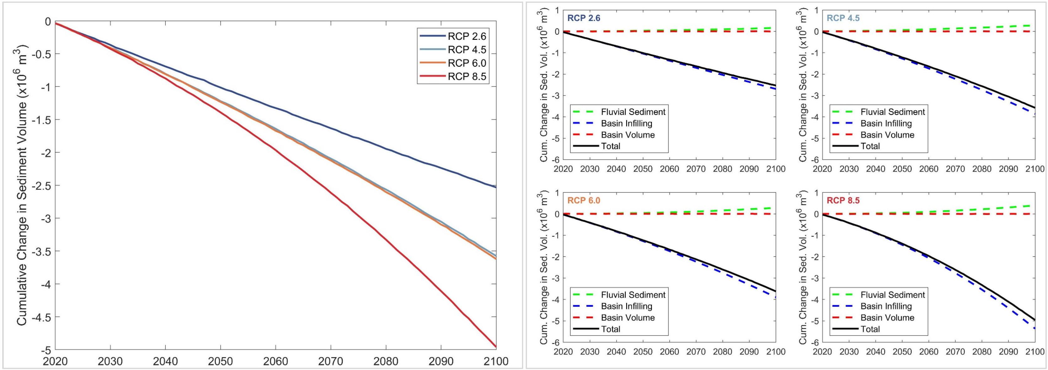
Figure 8. Projected change in total sediment volume exchange (ΔV_T) between the Dyfi estuary and the adjacent coast (left), and the relative contributions of the three different sediment volume components (right) over the 21^st century for RCP 2.6, 4.5, 6.0, and 8.5. Negative and positive values of ΔV_T indicate sediment imported to the estuary from the adjacent coast and sediment exported from the estuary to the adjacent coast, respectively.

FIGURE 9

Figure 9. Projected change in total sediment volume exchange (ΔV_T) between the Kalutara estuary and the adjacent coast (left), and the relative contributions of the three different sediment volume components (right) over the 21^st century for RCP 2.6, 4.5, 6.0, and 8.5. Negative and positive values of ΔV_T indicate sediment imported to the estuary from the adjacent coast and sediment exported from the estuary to the adjacent coast, respectively.

The model projections indicate that the Alsea estuary system will import sediment from its adjacent coast throughout the 21^st century. The maximum and minimum projected volumes of sediment imports by 2100 are −1.25 million cubic meters (MCM) (RCP 8.5) and −1.0 MCM (RCP 2.6). The results also indicate that ΔV_T at the Alsea estuary system is predominantly governed by the process of basin infilling (ΔV_BI) and that the projected variations of ΔV_BV have trivial impacts on ΔV_T for all RCPs. The increased supply of fluvial sediment toward the end-century period slightly reduce sediment demand due to basin infilling for all RCPs. These increases in fluvial sediment supply toward the end-of-the-century are governed by the projected increments in temperature (Table 2) and the increase in human-induced erosion factor.

The model projections indicate that the Dyfi estuary system will also import sediment from the adjacent coast throughout the 21^st century. The maximum and minimum projected volumes of sediment imports by 2100 are −5.0 MCM (RCP 8.5) and −2.5 MCM (RCP 2.6). The results here too indicate that ΔV_T at the Dyfi estuary system is governed by the basin sediment demand (ΔV_BI), while projected variations of ΔV_BV and ΔV_FS have trivial impacts on ΔV_T for all RCPs. The river catchment area of this CEC system is relatively small compared with the estuary surface area. Hence, despite the projected increments in temperature (Table 2) and the increase in human-induced erosion, fluvial sediment supply by the Dyfi River catchment contributes little to the sediment volume demand due to basin infilling for all RCPs.

The model projections indicate that the Kalutara estuary system will also import sediment from the adjacent coast throughout the 21^st century. The maximum and minimum projected volumes of sediment imports by 2100 are −7.0 MCM (RCP 2.6) and -3.0 MCM (RCP 8.5). The results here indicate that ΔV_T at the Kalutara estuary system is governed by the fluvial sediment supply (ΔV_FS), while projected variations of ΔV_BV and ΔV_BI have trivial impacts on ΔV_T for all RCPs. However, it should be noted that the fluvial sediment supply from the Kalu River catchment is significantly affected by river sand mining (Bamunawala et al., 2018b), which is taken into account in these simulations (423,000 m³/yr). Model projections show that, despite river sand mining, Kalutara estuary will export sediment to the adjacent coast during the end-century period for RCP 8.5. This is due to the significant increments of the projected T and Q (Table 2) over 2091–2100 (relative to the reference period), which substantially increases ΔV_FS, and to a lesser degree ΔV_BV.

Projected Coastline Change at the Case Study Locations: 2020–2100

The ΔV_T values computed in section “Model Hindcasts for the 1986–2005 Period” were used to determine the changes in the position of the coastlines adjacent to the three case studies (Figure 10).

FIGURE 10

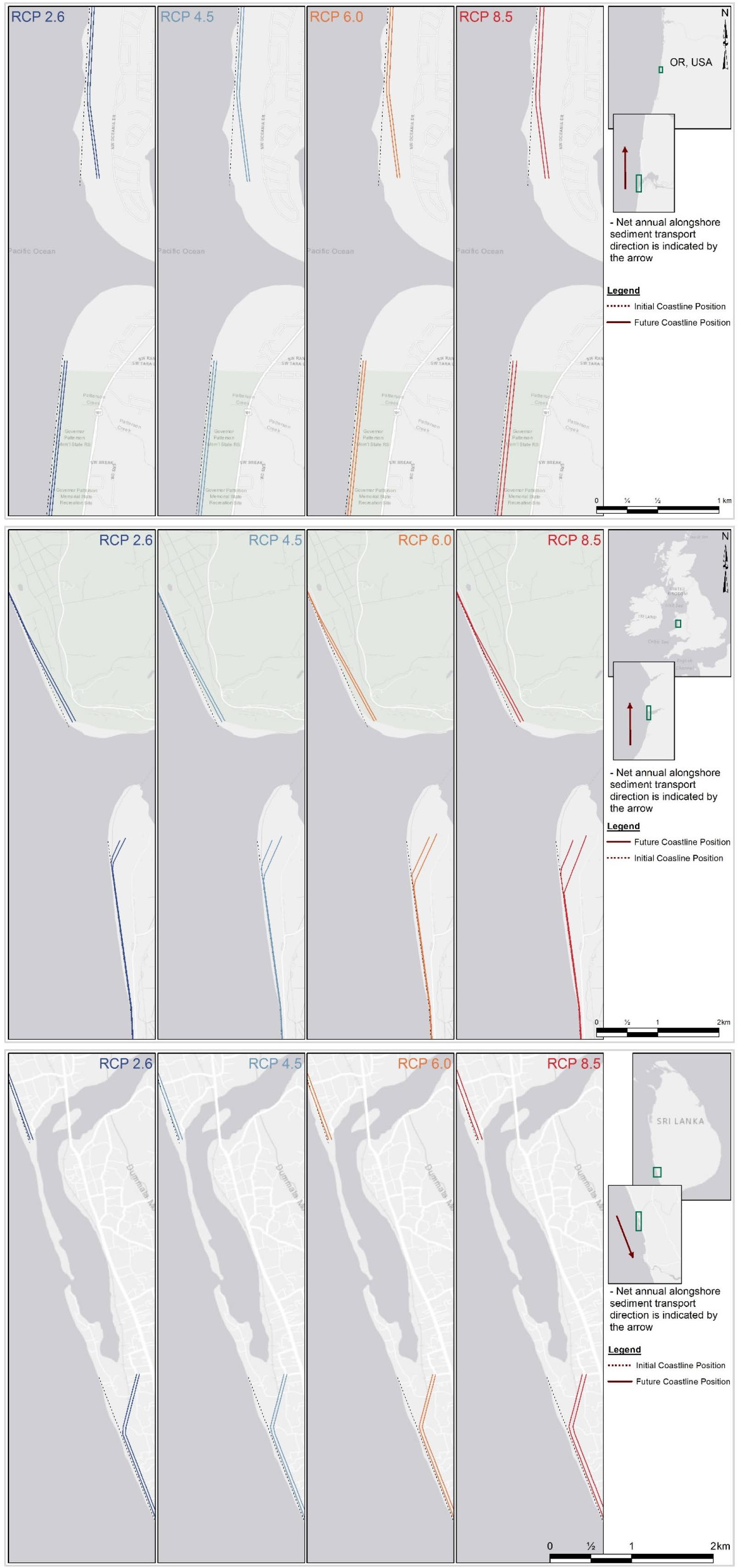
Figure 10. Projected changes of the coastline adjacent to the Alsea estuary (top), Dyfi estuary (middle), and Kalutara estuary (bottom). The two solid lines in each subplot represent the final coastline position by 2060 and 2100 (in the same order, moving landward from the most seaward line). The dotted line in each subplot represents the initial (reference) coastline position considered.

At the Alsea estuary, the sediment volume demand of the basin (i.e., ΔV_T) acts as a sink at the inlet. However, the magnitude of ΔV_T is smaller than the existing LST capacity at the inlet. Therefore, the down-drift coast will be subjected to additional coastline recession driven by the ΔV_T, over and above that due to the Bruun effect. The total recession along the down-drift coast may vary between 71 m (RCP 2.6) and 75 m (RCP 8.5) by 2100. The up-drift coast is only affected by the coastline recession due to the Bruun effect, which is projected to vary between 50 m (RCP 2.6) and 70 m (RCP 8.5) by 2100.

At the Dyfi estuary too, ΔV_T causes the inlet to act as a sediment sink. As the magnitude of ΔV_T here is greater than the existing LST capacity at the inlet, both the up- and down-drift coast should provide sediment to the basin. Thus, both the up- and down-drift coasts will be subjected to additional coastline recession driven by the ΔV_T, over and above that of Bruun effect. The extent of additional coastline recession along the down-drift coastline is constrained by the longshore sediment transport capacity while that along the up-drift coast corresponds to the deficit in sediment volume (i.e., the difference between the estuarine sediment demand and longshore sediment transport capacity). The model projections indicate that the down-drift coast at the Dyfi estuary may erode by 78 m (RCP 2.6) to 96 m (RCP 8.5) by 2100. However, the up-drift coast is projected to erode between 85 m (RCP 2.6) and 140 m (RCP 8.5) by 2100.

The Kalutara estuary is also projected to act as a sediment sink during all but the end-century period for RCP 8.5. Since these projected magnitudes of ΔV_T values are less than the existing LST capacity at the inlet, the down-drift coast will be subjected to additional coastline recession driven by ΔV_T, over and above the Bruun effect. Under RCP 8.5, the inlet acts as a sediment source during the end-century period, thus reducing recession due to Bruun effect along the down-drift coast. The projected coastline recession along the down-drift coast vary between 82 m (RCP 2.6) and 110 m (RCP 8.5) by 2100. The up-drift coast is only affected by the coastline recession due to the Bruun effect, which varies between 50 m (RCP 2.6) and 70 m (RCP 8.5) by 2100.

Discussion

Application of the newly developed model to the three barrier estuary case-studies indicates that macro-time-scale evolution of inlet-interrupted coasts under the influences of climate change-driven impacts and anthropogenic activities would vary markedly from system to system. Although the coastlines at these case study sites are projected to erode by the end of this century, the physical processes governing the erosion are different among the three systems.

Model projections show that the future sediment exchange between the estuary and the coast at both the Alsea and Dyfi estuary systems will be governed by the sediment demand due to basin infilling, although, the Alsea inlet system will also be partially influenced by fluvial sediment supply, especially toward the latter part of the 21^st century. Due to the small projected changes in annual cumulative river discharges and the size of the basin volumes, both these systems are not affected by the sediment demand due to variations in basin volume size.

The projected future sediment exchange behavior at the Kalutara estuary system is rather different and is governed by the fluvial sediment supply. Due to the combined effects of the projected increments in temperature and river discharge, and anthropogenic activities, the Kalutara river catchment may generate a surplus of sediment throughout the 21^st century. However, if the present practice of river sand mining continues, the catchment generated sediment surplus will be significantly reduced, resulting in eroding the adjacent coast. Due to the relatively small basin size (both volume and surface area), effects of sediment demand due to variations in basin volume size and basin infilling are negligible at the Kalutara CEC system.

The coastline change projections presented by Vousdoukas et al. (2020) indicate 50 m of erosion along both up-and down-drift coast of the Alsea estuary by 2100 for RCP 8.5. The same study indicates 100 and 150 m erosion along both up-and down-drift coast of the Dyfi estuary and Kalutara inlet, respectively for RCP 8.5 by 2100. It should, however, be noted that the global assessment of sandy coastline variation presented by Vousdoukas et al. (2020) does not consider any estuarine effects and also incorporates a correction factor for Bruun effect-driven coastline recession. As a result, the model projections of the present study will, by necessity, differ from the coastline variation presented by Vousdoukas et al. (2020) at the study locations.

In the model presented here, everything seaward of the shoreline is considered as the “outside world,” in order to avoid making this model over-complicated by bringing in complex ebb delta dynamics. Moreover, there are no significant ebb deltas in the three selected CEC systems. In general terms, the presence of ebb deltas would not affect the computation of sediment exchange volumes. However, if there is a significant ebb delta, in which the sand is mobile, part of the sediment demand of the inlet-estuary system (for an importing estuary) could be met by sand supply from the ebb delta. This will affect the coastline change projections by reducing the volume of sediment eroded from the coast. In such situations, the projections given by this model can be considered as pessimistic estimates of coastline recession. At sediment exporting inlet-estuary systems, part of the sediment supplied to the coast may contribute to the development of the ebb delta. Therefore, coastline changes projected by the model under these circumstances will over-predict coastline accretions (i.e., optimistic estimates).

It should also be noted that the simplified one-line coastline change model presented in this study only provides preliminary (i.e., first-order) estimates of variations along the inlet-interrupted coasts. This simplified modeling framework uses a relatively shallow profile (up to the depth of closure) and does not account for any local changes in coastline orientation (i.e., straight shoreline segments are assumed) or the presence of any coastal structures. In addition, for computational efficiency, the coastline change modeling used here treats the coastline up-drift and down-drift of the inlet separately, and as sequences of linear shoreline segments. This treatment results in a rather coarse representation of coastline change and does not resolve subtle coastline curvatures that are coupled with gradients in net alongshore sediment transport and shoreline change rates, which has implications for the way in which erosion or progradation might propagate along the coast. Coupling the terrestrial and estuarine model components with a coastline change model that is able to simulate more realistic changes in coastline shape and orientation [e.g., Coastline Evolution Model (CEM); Ashton and Murray, 2006; the Coastal One-line Vector Evolution Model (COVE); Hurst et al., 2015, or ShorelineS, Roelvink et al., 2020], will improve model predictions significantly. Usage of such a coastline change model will enable more realistic forecasts of changes in coastline shape and orientation, which equate to the capacity to predict shoreline-change hot spots, in response to future changes in wave climate (Slott et al., 2006; Hurst et al., 2015; Anderson et al., 2018; Antolínez et al., 2018). Besides, future changes in wave climate may also alter the in longshore sediment transport rates and gradients therein. Such variations in LST may affect the evolution of inlet-interrupted coasts and thus need to be considered via detailed site-specific assessments of coastline change.

Results of this study show that fundamental CEC system properties such as basin volume and surface area, river catchment area and projected climatic conditions over the river catchment are closely related to the long-term evolution of inlet-interrupted coasts. The existence of any generally applicable relationships/dependencies between these properties/forcing and coastline change could be investigated by applying the model presented here at a larger number of CEC systems with diverse environmental and geographical settings.

There are significant uncertainties in future climate change and anthropogenic activities that need to be borne in mind when considering the projections of coastline change provided here, especially at small tidal-inlet systems, which are highly sensitive to changes in forcing conditions. As a result [in addition to the uncertainties associated with the modeling technique(s) adopted], projections of inlet-interrupted coastline changes will inherit the variabilities in climate change forcing and anthropogenic activities (i.e., input uncertainties) considered. In some situations, for example, to inform catchment/coastal zone management decisions, it may be desirable to have a quantitative understanding of the separate contribution of climate change and anthropogenic activities to the total uncertainty of the coastline change projections. This may be achieved via a Variance Based Sensitivity Analysis (VBSA) using Sobol indices (Sobol’, 2001) as done by Le Cozannet et al. (2019).

Conclusion

A new model that can rapidly simulate the climate-change driven evolution of inlet-interrupted coasts at 50–100 year time scales, while taking into account the contributions from catchment-estuary-coastal systems in a holistic manner has been developed and piloted at three different case study locations. The spatio-temporal evolution of inlet-interrupted coasts is simulated by (1) computing the variation of total sediment volume exchange between the inlet-estuary system and its adjacent coast (ΔV_T), and (2) distributing the computed ΔV_T along the inlet-interrupted coast as a spatially and temporally varying quantity. The exchange volume ΔV_T is calculated as a function of variations in fluvial sediment supply (ΔV_FS), basin (or estuarine) infilling due to the sea-level rise-induced increase in accommodation space (ΔV_BI), and estuarine sediment volume change due to variations in river discharge (ΔV_BV).

The three case study locations considered in this study are: the Alsea estuary (Oregon, United States), Dyfi estuary (Wales, United Kingdom), and Kalutara inlet (Sri Lanka), which broadly represent some of the barrier estuary systems and geomorphic settings found across the world. The model was first validated at the three case study locations against the satellite image derived ambient shoreline change rates presented by Luijendijk et al. (2018) over 1986–2005. Subsequently, the model was applied in forecast mode at the case study sites, with the aim of investigating system behavior under projected climate-change impacts and anthropogenic activities.

Results indicated that all three systems will experience sediment deficits by 2100 (i.e., sediment importing estuaries) leading to coastline recession along the inlet-adjacent coasts. However, the processes and system characteristics governing the total sediment exchange volume, and thus coastline change, vary among the systems due to differences in geomorphic settings and projected climatic conditions. Therefore, the results of this study demonstrate the importance of carefully considering catchment and estuarine processes (i.e., fluvial sediment supply, basin infilling and basin volume change) in obtaining projections of coastline change at inlet-interrupted coasts at macro time scales.

Data Availability Statement

The raw data supporting the conclusions of this article will be made available by the authors, without undue reservation, to any qualified researcher.

Author Contributions

JB, AD, AS, and RR conceived and designed the study. JB developed the model, carried out all model applications, and wrote the first draft of the manuscript. SM provided specific guidance on the catchment hydrology aspects of the study. TD provided specific guidance on the SMIC model adaptation, and QA’d the new code. TS assisted with GCM data collection and catchment delineation. All authors provided feedback on the manuscript and contributed text.

Funding

This study was part of JB’s Ph.D. research which was supported by the Deltares research program “Understanding System Dynamics; from River Basin to Coastal Zone” and the AXA Research Fund.

Conflict of Interest

The authors declare that the research was conducted in the absence of any commercial or financial relationships that could be construed as a potential conflict of interest.

Acknowledgments

JB was supported by the Deltares research program “Understanding System Dynamics; from River Basin to Coastal Zone” and the AXA Research Fund. RR is supported by the AXA Research Fund and the Deltares Strategic Research Programme “Coastal and Offshore Engineering.” Last of the Wild Project, Global Human Footprint, Version 2 data were developed by the Wildlife Conservation Society – WCS and the Columbia University Center for International Earth Science Information Network (CIESIN), Columbia University and were obtained from the NASA Socioeconomic Data and Applications Center (SEDAC) at http://dx.doi.org/10.7927/H4M61H5F, accessed 1 October 2015. Any use of trade, firm, or product names is for descriptive purposes only and does not imply endorsement by the U.S. Government.

References

Anderson, D., Ruggiero, P., Antolínez, J. A. A., Méndez, F. J., and Allan, J. (2018). A climate index optimized for longshore sediment transport reveals interannual and multidecadal littoral cell rotations. J. Geophys. Res. Earth Surf. 123, 1958–1981. doi: 10.1029/2018JF004689

CrossRef Full Text | Google Scholar

Anthony, E. J., Besset, M., Dussouillez, P., Goichot, M., and Loisel, H. (2019). Overview of the Monsoon-influenced Ayeyarwady River delta, and delta shoreline mobility in response to changing fluvial sediment supply. Mar. Geol. 417:106038. doi: 10.1016/j.margeo.2019.106038

CrossRef Full Text | Google Scholar

Anthony, E. J., Brunier, G., Besset, M., Goichot, M., Dussouillez, P., and Nguyen, V. L. (2015). Linking rapid erosion of the Mekong River delta to human activities. Sci. Rep. 5:14745. doi: 10.1038/srep14745

PubMed Abstract | CrossRef Full Text | Google Scholar

Anthony, E. J., Gardel, A., Proisy, C., Fromard, F., Gensac, E., Peron, C., et al. (2013). The role of fluvial sediment supply and river-mouth hydrology in the dynamics of the muddy, Amazon-dominated Amapá–Guianas coast, South America: a three-point research agenda. J. South Am. Earth Sci. 44, 18–24. doi: 10.1016/j.jsames.2012.06.005

CrossRef Full Text | Google Scholar

Antolínez, J. A. A., Murray, A. B., Méndez, F. J., Moore, L. J., Farley, G., and Wood, J. (2018). Downscaling changing coastlines in a changing climate: the hybrid approach. J. Geophys. Res. Earth Surf. 123, 229–251. doi: 10.1002/2017JF004367

CrossRef Full Text | Google Scholar

Ashton, A. D., and Murray, A. B. (2006). High-angle wave instability and emergent shoreline shapes: 1. Modeling of sand waves, flying spits, and capes. J. Geophys. Res. Earth Surf. 111:F04012. doi: 10.1029/2005JF000422

CrossRef Full Text | Google Scholar

Athanasiou, P., van Dongeren, A., Giardino, A., Vousdoukas, M., Gaytan-Aguilar, S., and Ranasinghe, R. (2019). Global distribution of nearshore slopes with implications for coastal retreat. Earth Syst. Sci. Data Discuss. 2019, 1–29. doi: 10.5194/essd-2019-71

CrossRef Full Text | Google Scholar

Aubrey, D. G., and Weishar, L. (eds) (1988). Hydrodynamics and Sediment Dynamics of Tidal Inlets. New York, NY: Springer.

Google Scholar

Baart, F., Gelder, P. H. A. J. M., van Ronde, J., de Koningsveld, M., and van Wouters, B. (2012). The effect of the 18.6-year lunar nodal cycle on regional sea-level rise estimates. J. Coast. Res. 28, 511–516. doi: 10.2112/JCOASTRES-D-11-00169.1

CrossRef Full Text | Google Scholar

Balthazar, V., Vanacker, V., Girma, A., Poesen, J., and Golla, S. (2013). Human impact on sediment fluxes within the Blue Nile and Atbara River basins. Geomorphology 180–181, 231–241. doi: 10.1016/j.geomorph.2012.10.013

CrossRef Full Text | Google Scholar

Bamunawala, J., Maskey, S., Duong, T., and van der Spek, A. (2018a). Significance of fluvial sediment supply in coastline modelling at tidal inlets. J. Mar. Sci. Eng. 6:79. doi: 10.3390/jmse6030079

CrossRef Full Text | Google Scholar

Bamunawala, J., Ranasinghe, R., van der Spek, A., Maskey, S., and Udo, K. (2018b). Assessing future coastline change in the vicinity of tidal inlets via reduced complexity modelling. J. Coast. Res. 85, 636–640. doi: 10.2112/SI85-128.1

CrossRef Full Text | Google Scholar

Barnard, P. L., Foxgrover, A. C., Elias, E. P. L., Erikson, L. H., Hein, J. R., McGann, M., et al. (2013a). Integration of bed characteristics, geochemical tracers, current measurements, and numerical modeling for assessing the provenance of beach sand in the San Francisco Bay Coastal System. Mar. Geol. 336, 120–145. doi: 10.1016/j.margeo.2012.11.008

CrossRef Full Text | Google Scholar

Barnard, P. L., Hansen, J. E., and Erikson, L. H. (2012). Synthesis study of an erosion hot spot, ocean beach, California. J. Coast. Res. 28, 903–922. doi: 10.2112/JCOASTRES-D-11-00212.1

CrossRef Full Text | Google Scholar

Barnard, P. L., and Kvitek, R. G. (2010). Anthropogenic influence on recent bathymetric change in West-Central San Francisco Bay. San Fr. Estuary Watershed Sci. 8:13. doi: 10.15447/sfews.2010v8iss3art2

CrossRef Full Text | Google Scholar

Barnard, P. L., Schoellhamer, D. H., Jaffe, B. E., and McKee, L. J. (2013b). Sediment transport in the San Francisco Bay coastal system: an overview. Mar. Geol. 345, 3–17. doi: 10.1016/j.margeo.2013.04.005

CrossRef Full Text | Google Scholar

Bayram, A., Larson, M., and Hanson, H. (2007). A new formula for the total longshore sediment transport rate. Coast. Eng. 54, 700–710. doi: 10.1016/j.coastaleng.2007.04.001

CrossRef Full Text | Google Scholar

Besset, M., Anthony, E. J., and Bouchette, F. (2019). Multi-decadal variations in delta shorelines and their relationship to river sediment supply: an assessment and review. Earth Sci. Rev. 193, 199–219. doi: 10.1016/j.earscirev.2019.04.018

CrossRef Full Text | Google Scholar

Bruun, P. M. (1962). Sea-level rise as a cause of shore erosion. Am. Soc. Civ. Eng. Proc. J. Waterw. Harb. Div. 88, 117–132.

Google Scholar

Casas-Prat, M., and Sierra, J. P. (2013). Projected future wave climate in the NW Mediterranean Sea. J. Geophys. Res. Ocean. 118, 3548–3568. doi: 10.1002/jgrc.20233

CrossRef Full Text | Google Scholar

Casas-Prat, M., Wang, X. L., and Swart, N. (2018). CMIP5-based global wave climate projections including the entire Arctic Ocean. Ocean Model. 123, 66–85. doi: 10.1016/j.ocemod.2017.12.003

CrossRef Full Text | Google Scholar

CERC (1984). Shore Protection Manual. Washington, DC: CERC.

Google Scholar

Chu, Z. (2014). The dramatic changes and anthropogenic causes of erosion and deposition in the lower Yellow (Huanghe) River since 1952. Geomorphology 216, 171–179. doi: 10.1016/j.geomorph.2014.04.009

CrossRef Full Text | Google Scholar

Cowell, P. J., Stive, M. J. F., Niedoroda, A. W., De-Vriend, H. J., Swift, D. J. P., Kaminsky, G. M., et al. (2003). The coastal-tract (Part 1): a conceptual approach to aggregated modeling of low-order coastal change. J. Coast. Res. 19, 812–827.

Google Scholar

CSIRO, and Bureau of Meteorology (2015). Climate Change in Australia Information for Australia’s Natural Resource Management Regions: Technical Report. Australia: CSIRO and Bureau of Meteorology.

Google Scholar

Dallas, K. L., and Barnard, P. L. (2011). Anthropogenic influences on shoreline and nearshore evolution in the San Francisco Bay coastal system. Estuar. Coast. Shelf Sci. 92, 195–204. doi: 10.1016/j.ecss.2010.12.031

CrossRef Full Text | Google Scholar

Dalrymple, R. W. (1992). “‘Tidal depositional systems’,” in Facies Models: Response to Sea Level Change, eds R. G. Walker and N. P. James (St John’s: Geological Association of Canada), 195–218.

Google Scholar

Dalrymple, R. W., and Choi, K. (2007). Morphologic and facies trends through the fluvial–marine transition in tide-dominated depositional systems: a schematic framework for environmental and sequence-stratigraphic interpretation. Earth Sci. Rev. 81, 135–174. doi: 10.1016/j.earscirev.2006.10.002

CrossRef Full Text | Google Scholar

Dalrymple, R. W., and Choi, K. S. (2003). “‘Sediment transport by tides’,” in Encyclopedia of Sediments and Sedimentary Rocks, ed. G. V. Middleton (Dordrecht: Springer), 606–609.

Google Scholar

Dastgheib, A., Reyns, J., Thammasittirong, S., Weesakul, S., Thatcher, M., and Ranasinghe, R. (2016). Variations in the wave climate and sediment transport due to climate change along the coast of vietnam. J. Mar. Sci. Eng. 4:86. doi: 10.3390/jmse4040086

CrossRef Full Text | Google Scholar

Davis, R. A. Jr., and Fitzgerald, D. M. (2003). Beaches and Coasts. Hoboken, NJ: Wiley-Blackwell.

Google Scholar

Davis, R. A. (1989). “Morphodynamics of the West-Central Florida barrier system: the delicate balance between wave- and tide-domination,” in Coastal Lowlands: Geology and Geotechnology, eds W. J. M. van der Linden, S. A. P. L. Cloetingh, J. P. K. Kaasschieter, W. J. E. van de Graaff, J. Vandenberghe, and J. A. M. van der Gun (Dordrecht: Springer), 225–235. doi: 10.1007/978-94-017-1064-0_15

CrossRef Full Text | Google Scholar

Davis, R. A., and Barnard, P. (2003). Morphodynamics of the barrier-inlet system, west-central Florida. Mar. Geol. 200, 77–101. doi: 10.1016/S0025-3227(03)00178-6

CrossRef Full Text | Google Scholar

Davis, R. A., and Barnard, P. L. (2000). How anthropogenic factors in the back-barrier area influence tidal inlet stability: examples from the Gulf Coast of Florida, USA. Geol. Soc. Lond. Spec. Publ. 175, 293–303. doi: 10.1144/GSL.SP.2000.175.01.21

CrossRef Full Text | Google Scholar

Davis, R. A., and Fox, W. T. (1981). Interaction between wave- and tide-generated processes at the mouth of a microtidal estuary: matanzas River, Florida (U.S.A.). Mar. Geol. 40, 49–68. doi: 10.1016/0025-3227(81)90042-6

CrossRef Full Text | Google Scholar

Davis, R. A., and Hayes, M. O. (1984). What is a wave-dominated coast? Mar. Geol. 60, 313–329. doi: 10.1016/0025-3227(84)90155-5

CrossRef Full Text | Google Scholar

Dronkers, J. J. (1964). Tidal Computations in Rivers and Coastal Waters. New York, NY: North-Holland Pub. Co.

Google Scholar

Dunn, F. E., Darby, S. E., Nicholls, R. J., Cohen, S., Zarfl, C., and Fekete, B. M. (2019). Projections of declining fluvial sediment delivery to major deltas worldwide in response to climate change and anthropogenic stress. Environ. Res. Lett. 14:84034. doi: 10.1088/1748-9326/ab304e

CrossRef Full Text | Google Scholar

Dunn, F. E., Nicholls, R. J., Darby, S. E., Cohen, S., Zarfl, C., and Fekete, B. M. (2018). Projections of historical and 21^st century fluvial sediment delivery to the Ganges-Brahmaputra-Meghna, Mahanadi, and Volta deltas. Sci. Total Environ. 642, 105–116. doi: 10.1016/j.scitotenv.2018.06.006

PubMed Abstract | CrossRef Full Text | Google Scholar

Duong, T. M. (2015). Climate Change Impacts on the Stability of Small Tidal Inlets. Delft: Delft University of Technology.

Google Scholar

Duong, T. M., Ranasinghe, R., Luijendijk, A., Walstra, D., and Roelvink, D. (2017). Assessing climate change impacts on the stability of small tidal inlets: part 1 - Data poor environments. Mar. Geol. 390, 331–346. doi: 10.1016/j.margeo.2017.05.008

CrossRef Full Text | Google Scholar

Duong, T. M., Ranasinghe, R., Thatcher, M., Mahanama, S., Wang, Z. B., Dissanayake, P. K., et al. (2018). Assessing climate change impacts on the stability of small tidal inlets: part 2 - Data rich environments. Mar. Geol. 395, 65–81. doi: 10.1016/j.margeo.2017.09.007

PubMed Abstract | CrossRef Full Text | Google Scholar

Duong, T. M., Ranasinghe, R., Walstra, D., and Roelvink, D. (2016). Assessing climate change impacts on the stability of small tidal inlet systems: why and how? Earth Sci. Rev. 154, 369–380. doi: 10.1016/j.earscirev.2015.12.001

CrossRef Full Text | Google Scholar

Ericson, J. P., Vörösmarty, C. J., Dingman, S. L., Ward, L. G., and Meybeck, M. (2006). Effective sea-level rise and deltas: causes of change and human dimension implications. Glob. Planet. Change 50, 63–82. doi: 10.1016/j.gloplacha.2005.07.004

CrossRef Full Text | Google Scholar

Erikson, L. H., Hegermiller, C. A., Barnard, P. L., Ruggiero, P., and van Ormondt, M. (2015). Projected wave conditions in the Eastern North Pacific under the influence of two CMIP5 climate scenarios. Ocean Model. 96, 171–185. doi: 10.1016/j.ocemod.2015.07.004

CrossRef Full Text | Google Scholar

Farr, T. G., Rosen, P. A., Caro, E., Crippen, R., Duren, R., Hensley, S., et al. (2007). The shuttle radar topography mission. Rev. Geophys. 45:RG2004. doi: 10.1029/2005RG000183

CrossRef Full Text | Google Scholar

FitzGerald, D., Georgiou, I., and Miner, M. (2015). “Estuaries and tidal inlets,” in Coastal Environments and Global Change Wiley Online Books, eds G. Masselink and R. Gehrels (Chichester, UK: John Wiley & Sons, Ltd), 268–298. doi: 10.1002/9781119117261.ch12

CrossRef Full Text | Google Scholar

FitzGerald, D. M., Georgiou, I., and Miner, M. (2014). “Estuaries and tidal inlets,” in Coastal Environments and Global Change, eds G. Masselink and R. Gehrels (Sussex: John Wiley & Sons, Ltd and American Geophysical Union), 268–298. doi: 10.1002/9781119117261.ch12

CrossRef Full Text | Google Scholar

French, J., Payo, A., Murray, B., Orford, J., Eliot, M., and Cowell, P. (2016). Appropriate complexity for the prediction of coastal and estuarine geomorphic behaviour at decadal to centennial scales. Geomorphology 256, 3–16. doi: 10.1016/j.geomorph.2015.10.005

CrossRef Full Text | Google Scholar

Gao, S., and Collins, M. (1994). Tidal inlet equilibrium, in relation to cross-sectional area and sediment transport patterns. Estuar. Coast. Shelf Sci. 38, 157–172. doi: 10.1006/ecss.1994.1010

CrossRef Full Text | Google Scholar

Grabemann, I., Groll, N., Möller, J., and Weisse, R. (2015). Climate change impact on North Sea wave conditions: a consistent analysis of ten projections. Ocean Dyn. 65, 255–267. doi: 10.1007/s10236-014-0800-z

CrossRef Full Text | Google Scholar

Green, M. O. (2013). Catchment sediment load limits to achieve estuary sedimentation targets. New Zeal. J. Mar. Freshw. Res. 47, 153–180. doi: 10.1080/00288330.2012.757241

CrossRef Full Text | Google Scholar

Hayes, M. O. (1980). General morphology and sediment patterns in tidal inlets. Sediment. Geol. 26, 139–156. doi: 10.1016/0037-0738(80)90009-3

CrossRef Full Text | Google Scholar

Hemer, M. A., Fan, Y., Mori, N., Semedo, A., and Wang, X. L. (2013). Projected changes in wave climate from a multi-model ensemble. Nat. Clim. Chang. 3, 471–476. doi: 10.1038/nclimate1791

CrossRef Full Text | Google Scholar

Hemer, M. A., McInnes, K. L., and Ranasinghe, R. (2012). Climate and variability bias adjustment of climate model-derived winds for a southeast Australian dynamical wave model. Ocean Dyn. 62, 87–104. doi: 10.1007/s10236-011-0486-4

CrossRef Full Text | Google Scholar

Hume, T. M., and Herdendorf, C. E. (1993). On the use of empirical stability relationships for characterising estuaries. J. Coast. Res. 9, 413–422.

Google Scholar

Hurst, M. D., Barkwith, A., Ellis, M. A., Thomas, C. W., and Murray, A. B. (2015). Exploring the sensitivities of crenulate bay shorelines to wave climates using a new vector-based one-line model. J. Geophys. Res. Earth Surf. 120, 2586–2608. doi: 10.1002/2015JF003704

CrossRef Full Text | Google Scholar

Kamphuis, J. W. (1991). Alongshore sediment transport rate. J. Waterw. Port Coast. Ocean Eng. 117, 624–640. doi: 10.1061/(ASCE)0733-950X1991117:6(624)

CrossRef Full Text | Google Scholar

Kettner, A. J., Syvitski, J. P., and Gomez, B. (2005). “Simulating the effects of natural events and anthropogenic activity on sediment discharge to the poverty shelf, new zealand during the late holocene,” in Proceedings of the Eos Trans. AGU, 86(52), Fall Meet. Suppl., Abstract H51C-0388 (Washington, DC: IEEE).

Google Scholar

Keulegan, G. H. (1951). Third Progress Report on Tidal Flow in Entrances, Water Level Fluctuations of Basins in Communication with Seas. Report No. 1146. Washington D.C: National Bureau of Standards.

Google Scholar

Le Cozannet, G., Bulteau, T., Castelle, B., Ranasinghe, R., Wöppelmann, G., Rohmer, J., et al. (2019). Quantifying uncertainties of sandy shoreline change projections as sea level rises. Sci. Rep. 9:42. doi: 10.1038/s41598-018-37017-4

PubMed Abstract | CrossRef Full Text | Google Scholar

Luijendijk, A., Hagenaars, G., Ranasinghe, R., Baart, F., Donchyts, G., and Aarninkhof, S. (2018). The State of the World’s beaches. Sci. Rep. 8:6641. doi: 10.1038/s41598-018-24630-6

PubMed Abstract | CrossRef Full Text | Google Scholar

McGranahan, G., Balk, D., and Anderson, B. (2007). The rising tide: assessing the risks of climate change and human settlements in low elevation coastal zones. Environ. Urban 19, 17–37. doi: 10.1177/0956247807076960

CrossRef Full Text | Google Scholar

McSweeney, S. L., Kennedy, D. M., Rutherfurd, I. D., and Stout, J. C. (2017). Intermittently Closed/Open Lakes and Lagoons: their global distribution and boundary conditions. Geomorphology 292, 142–152. doi: 10.1016/j.geomorph.2017.04.022

CrossRef Full Text | Google Scholar

Mehvar, A., Dastgheib, A., and Ranasinghe, R. (2016). Relative Sea Level Rise Scenarios: Central Coast of Bangladesh. Delft: Delft University of Technology.

Google Scholar

Mori, N., Yasuda, T., Mase, H., Tom, T., and Oku, Y. (2010). Projection of extreme wave climate change under global warming. Hydrol. Res. Lett. 4, 15–19. doi: 10.3178/hrl.4.15

PubMed Abstract | CrossRef Full Text | Google Scholar

Morim, J., Hemer, M., Wang, X. L., Cartwright, N., Trenham, C., Semedo, A., et al. (2019). Robustness and uncertainties in global multivariate wind-wave climate projections. Nat. Clim. Chang. 9, 711–718. doi: 10.1038/s41558-019-0542-5

CrossRef Full Text | Google Scholar

Murray, A. B. (2007). Reducing model complexity for explanation and prediction. Geomorphology 90, 178–191. doi: 10.1016/j.geomorph.2006.10.020

CrossRef Full Text | Google Scholar

Murray, A. B. (2013). “‘Which models are good (enough), and when?’,” in Treatise on Geomorphology, ed. J. F. Shroder (Oxford: Elsevier-Academic Press), 50–58. doi: 10.1016/b978-0-12-374739-6.00027-0

CrossRef Full Text | Google Scholar

National Rivers Authority Welsh Region (1995). Dyfi and Leri Catchment Management Plan Consultation Report. Bristol: National Rivers Authority Welsh Region.

Google Scholar

Neumann, B., Vafeidis, A. T., Zimmermann, J., and Nicholls, R. J. (2015). Future coastal population growth and exposure to sea-level rise and coastal flooding - a global assessment. PLoS One 10:e0118571. doi: 10.1371/journal.pone.0118571

PubMed Abstract | CrossRef Full Text | Google Scholar

Nicholls, R. J., Hanson, S. E., Lowe, J. A., Warrick, R. A., Lu, X., and Long, A. J. (2014). Sea-level scenarios for evaluating coastal impacts. Wiley Interdiscip. Rev. Clim. Chang. 5, 129–150. doi: 10.1002/wcc.253

CrossRef Full Text | Google Scholar

O’Brien, M. P. (1969). Equilibrium flow areas of tidal inlets on sandy coasts. J. Waterw. Harb. Div. 95, 43–52.

Google Scholar

O’Neil, D. J. (1987). Variations in Alsea River Flow; Implications for Alsea Spit & Inlet Stability. Department of Geography, Oregon State University, Oregon.

Google Scholar

Oppenheimer, M., Glavovic, B. C., Hinkel, J., Van-de-Wal, R., Magnan, A. K., Abd-Elgawad, A., et al. (2019). “Sea level rise and implications for low-lying islands, coasts and communities,” in IPCC Special Report on the Ocean and Cryosphere in a Changing Climate, eds H.-O. Pörtner, D. C. Roberts, V. Masson-Delmotte, P. Zhai, M. Tignor, and E. Poloczanska (Geneva: IPCC).

Google Scholar

Overeem, I., Kettner, A. J., and Syvitski, J. P. M. (2013). “Impacts of humans on river fluxes and morphology,” in Treatise on Geomorphology, eds J. F. Shroder, and E. Wohl (Amsterdam: Elsevier), 828–842. doi: 10.1016/b978-0-12-374739-6.00267-0

CrossRef Full Text | Google Scholar

Overeem, I., and Syvitski, J. P. M. (2009). Dynamics and Vulnerability of Delta Systems. Geesthacht: GKSS Research Center. LOICZ Reports & Studies No. 35.

Google Scholar

Palmer, M. A., Liermann, C. A. R., Nilsson, C., Flörke, M., Alcamo, J., Lake, P. S., et al. (2008). Climate change and the world’s river basins: anticipating management options. Front. Ecol. Environ. 6, 81–89. doi: 10.1890/060148

CrossRef Full Text | Google Scholar

Paola, C. (2000). Quantitative models of sedimentary basin filling. Sedimentology 47, 121–178. doi: 10.1046/j.1365-3091.2000.00006.x

CrossRef Full Text | Google Scholar

Peng, D., Hill, E. M., Meltzner, A. J., and Switzer, A. D. (2019). Tide Gauge Records Show That the 18.61-Year Nodal Tidal Cycle Can Change High Water Levels by up to 30 cm. J. Geophys. Res. Ocean. 124, 736–749. doi: 10.1029/2018JC014695

CrossRef Full Text | Google Scholar

Pickering, M. D., Horsburgh, K. J., Blundell, J. R., Hirschi, J. J.-M., Nicholls, R. J., Verlaan, M., et al. (2017). The impact of future sea-level rise on the global tides. Cont. Shelf Res. 142, 50–68. doi: 10.1016/j.csr.2017.02.004

CrossRef Full Text | Google Scholar

Ranasinghe, R. (2016). Assessing climate change impacts on open sandy coasts: a review. Earth Sci. Rev. 160, 320–332. doi: 10.1016/j.earscirev.2016.07.011

CrossRef Full Text | Google Scholar

Ranasinghe, R. (2020). On the need for a new generation of coastal change models for the 21^st century. Sci. Rep. 10:2010. doi: 10.1038/s41598-020-58376-x

PubMed Abstract | CrossRef Full Text | Google Scholar

Ranasinghe, R., Duong, T. M., Uhlenbrook, S., Roelvink, D., and Stive, M. (2013). Climate-change impact assessment for inlet-interrupted coastlines. Nat. Clim. Chang. 3, 83–87. doi: 10.1038/nclimate1664

CrossRef Full Text | Google Scholar

Ranasinghe, R., Pattiaratchi, C., and Masselink, G. (1999). A morphodynamic model to simulate the seasonal closure of tidal inlets. Coast. Eng. 37, 1–36. doi: 10.1016/S0378-3839(99)00008-3

CrossRef Full Text | Google Scholar

Ranasinghe, R., Wu, C. S., Conallin, J., Duong, T. M., and Anthony, E. J. (2019). Disentangling the relative impacts of climate change and human activities on fluvial sediment supply to the coast by the world’s large rivers: pearl River Basin, China. Sci. Rep. 9:9236. doi: 10.1038/s41598-019-45442-2

PubMed Abstract | CrossRef Full Text | Google Scholar

Roelvink, D., Huisman, B., Elghandour, A., Ghonim, M., and Reyns, J. (2020). Efficient modeling of complex sandy coastal evolution at monthly to century time scales. Front. Mar. Sci. doi: 10.3389/fmars.2020.00535

CrossRef Full Text | Google Scholar

Samaras, A. G., and Koutitas, C. G. (2012). An integrated approach to quantify the impact of watershed management on coastal morphology. Ocean Coast. Manag. 69, 68–77. doi: 10.1016/j.ocecoaman.2012.08.010

CrossRef Full Text | Google Scholar

Sanderson, E. W., Jaiteh, M., Levy, M., Redford, K. H., Wannebo, A. V., and Woolmer, G. (2002). The Human Footprint and the Last of the Wild. Bioscience 52, 891–904.

Google Scholar

Semedo, A., Weisse, R., Behrens, A., Sterl, A., Bengtsson, L., and Günther, H. (2013). Projection of global wave climate change toward the end of the Twenty-First Century. J. Clim. 26, 8269–8288. doi: 10.1175/JCLI-D-12-00658.1

CrossRef Full Text | Google Scholar

Shennan, I., Coulthard, T., Flather, R., Horton, B., Macklin, M., Rees, J., et al. (2003). Integration of shelf evolution and river basin models to simulate Holocene sediment dynamics of the Humber Estuary during periods of sea-level change and variations in catchment sediment supply. Sci. Total Environ. 31, 737–754. doi: 10.1016/S0048-9697(03)00081-0

CrossRef Full Text | Google Scholar

Shimura, T., Mori, N., and Hemer, M. A. (2016). Variability and future decreases in winter wave heights in the Western North Pacific. Geophys. Res. Lett. 43, 2716–2722. doi: 10.1002/2016GL067924

CrossRef Full Text | Google Scholar

Shrestha, B., Babel, M. S., Maskey, S., van Griensven, A., Uhlenbrook, S., Green, A., et al. (2013). Impact of climate change on sediment yield in the Mekong River basin: a case study of the Nam Ou basin, Lao PDR. Hydrol. Earth Syst. Sci. 17, 1–20. doi: 10.5194/hess-17-1-2013

CrossRef Full Text | Google Scholar

Slagel, M. J., and Griggs, G. B. (2008). Cumulative Losses of Sand to the California Coast by Dam Impoundment. J. Coast. Res. 243, 571–584. doi: 10.2112/06-0640.1

CrossRef Full Text | Google Scholar

Slott, J. M., Murray, A. B., Ashton, A. D., and Crowley, T. J. (2006). Coastline responses to changing storm patterns. Geophys. Res. Lett. 33:L18404. doi: 10.1029/2006GL027445

CrossRef Full Text | Google Scholar

Sobol, I. M. (2001). Global sensitivity indices for nonlinear mathematical models and their Monte Carlo estimates. Math. Comput. Simul. 55, 271–280. doi: 10.1016/S0378-4754(00)00270-6

CrossRef Full Text | Google Scholar

Stive, M. J. F. (2004). How important is global warming for coastal erosion? Clim. Change 64, 27–39. doi: 10.1023/B:CLIM.0000024785.91858.1d

CrossRef Full Text | Google Scholar

Stive, M. J. F., Capobianco, M., Wang, Z. B., Ruol, P., and Buijsman, M. C. (1998). “‘Morphodynamics of a tidal lagoon and the adjacent coast’,” in Physics of Estuaries and Coastal Seas, eds J. Dronkers and M. Scheffers (Rotterdam: A. A. Balkema), 397–407.

Google Scholar

Stive, M. J. F., and Wang, Z. B. (2003). “‘Morphodynamic modeling of tidal basins and coastal inlets’,” in Advances in Coastal Modeling, ed. V. C. B. T.-E. O. S. Lakhan (Oxford: Elsevier), 367–392. doi: 10.1016/s0422-9894(03)80130-7

CrossRef Full Text | Google Scholar

Stocker, T. F., Qin, D., Plattner, G.-K., Alexander, L. V., Allen, S. K., Bindoff, N. L., et al. (2013a). “Technical summary,” in Climate Change 2013: The Physical Science Basis. Contribution of Working Group I to the Fifth Assessment Report of the Intergovernmental Panel on Climate Change, eds T. F. Stocker, D. Qin, G.-K. Plattner, M. Tignor, S. K. Allen, J. Boschung, et al. (Cambridge, MA: Cambridge University Press).

Google Scholar

Stocker, T. F., Qin, D., Plattner, G.-K., Tignor, M., Allen, S. K., and Boschung, J., et al. (eds) (2013b). “IPCC, 2013: summary for policymakers,” in Climate Change 2013: The Physical Science Basis. Contribution of Working Group I to the Fifth Assessment Report of the Intergovernmental Panel on Climate Change (Cambridge: Cambridge University Press).

Google Scholar

Syvitski, J. P. M. (2005). Impact of humans on the flux of terrestrial sediment to the Global Coastal Ocean. Science 308, 376–380. doi: 10.1126/science.1109454

PubMed Abstract | CrossRef Full Text | Google Scholar

Syvitski, J. P. M. (2008). Deltas at risk. Sustain. Sci. 3, 23–32. doi: 10.1007/s11625-008-0043-3

CrossRef Full Text | Google Scholar

Syvitski, J. P. M., Kettner, A. J., Overeem, I., Hutton, E. W. H., Hannon, M. T., Brakenridge, G. R., et al. (2009). Sinking deltas due to human activities. Nat. Geosci. 2, 681–686. doi: 10.1038/ngeo629

CrossRef Full Text | Google Scholar

Syvitski, J. P. M., and Milliman, J. D. (2007). Geology, geography, and humans battle for dominance over the delivery of fluvial sediment to the Coastal Ocean. J. Geol. 115, 1–19. doi: 10.1086/509246

CrossRef Full Text | Google Scholar

Syvitski, J. P. M., Peckham, S. D., Hilberman, R., and Mulder, T. (2003). Predicting the terrestrial flux of sediment to the global ocean: a planetary perspective. Sediment. Geol. 162, 5–24. doi: 10.1016/S0037-0738(03)00232-X

CrossRef Full Text | Google Scholar

Syvitski, J. P. M., and Saito, Y. (2007). Morphodynamics of deltas under the influence of humans. Glob. Planet. Change 57, 261–282. doi: 10.1016/j.gloplacha.2006.12.001

CrossRef Full Text | Google Scholar

Szabo, S., Brondizio, E., Renaud, F. G., Hetrick, S., Nicholls, R. J., Matthews, Z., et al. (2016). Population dynamics, delta vulnerability and environmental change: comparison of the Mekong, Ganges–Brahmaputra and Amazon delta regions. Sustain. Sci. 11, 539–554. doi: 10.1007/s11625-016-0372-6

PubMed Abstract | CrossRef Full Text | Google Scholar

Tessler, Z. D., Vorosmarty, C. J., Grossberg, M., Gladkova, I., Aizenman, H., Syvitski, J. P. M., et al. (2015). Profiling risk and sustainability in coastal deltas of the world. Science 349, 638–643. doi: 10.1126/science.aab3574

PubMed Abstract | CrossRef Full Text | Google Scholar

Townend, I. (2005). An examination of empirical stability relationships for UK estuaries. J. Coast. Res. 2005, 1042–1053. doi: 10.2112/03-0066R.1

CrossRef Full Text | Google Scholar

Veerbeek, W. (2017). Estimating the Impacts of Urban Growth on Future Flood Risk: A Comparative Study. Delft: Delft University of Technology.

Google Scholar

Verstraeten, G., and Poesen, J. (2001). Factors controlling sediment yield from small intensively cultivated catchments in a temperate humid climate. Geomorphology 40, 123–144. doi: 10.1016/S0169-555X(01)00040-X

CrossRef Full Text | Google Scholar

Vörösmarty, C. J., Meybeck, M., Fekete, B., Sharma, K., Green, P., and Syvitski, J. P. M. (2003). Anthropogenic sediment retention: major global impact from registered river impoundments. Glob. Planet. Change 39, 169–190. doi: 10.1016/S0921-8181(03)00023-7

CrossRef Full Text | Google Scholar

Vousdoukas, M. I., Ranasinghe, R., Mentaschi, L., Plomaritis, T. A., Athanasiou, P., Luijendijk, A., et al. (2020). Sandy coastlines under threat of erosion. Nat. Clim. Chang. 10, 260–263. doi: 10.1038/s41558-020-0697-0

CrossRef Full Text | Google Scholar

Walling, D. E. (2009). The Impact of Global Change on Erosion and Sediment Transport by Rivers: Current Progress and Future Challenges. The United Nations World Water Development Report 3 Water in a Changing World. Paris: UNESCO-IHP.

Google Scholar

Wildlife Conservation Society [WCS], and Columbia University Center for International Earth Science Information Network [CIESIN] (2005). Last of the Wild Project, Version 2, 2005 (LWP-2): Global Human Footprint Dataset (Geographic). Palisades, NY: CIESIN.

Google Scholar

Wolf, J., Lowe, J., and Howard, T. (2015). “Climate downscaling: local mean sea level, surge and wave modelling,” in Broad Scale Coastal Simulation. Advances in Global Change Research, eds R. J. Nicholls, R. Dawson, and S. Day (Dordrecht: Springer), 79–102. doi: 10.1007/978-94-007-5258-0_2

CrossRef Full Text | Google Scholar

Wong, P. P., Losada, I. J., Gattuso, J.-P., Hinkel, J., Khattabi, A., McInnes, K. L., et al. (2014). “‘Coastal systems and low-lying areas’,” in Climate Change 2014: Impacts, Adaptation, and Vulnerability. Part A: Global and Sectoral Aspects. Contribution of Working Group II to the Fifth Assessment Report of the Intergovernmental Panel on Climate Change, eds C. B. Field, V. R. Barros, D. J. Dokken, K. J. Mach, M. D. Mastrandrea, T. E. Bilir, et al. (Cambridge: Cambridge University Press), 361–409.

Google Scholar

Woodroffe, C. D. (2003). Coasts: Form, Process and Evolution. Cambridge, MA: Cambridge University Press.

Google Scholar

Yang, H. F., Yang, S. L., Xu, K. H., Milliman, J. D., Wang, H., Yang, Z., et al. (2018). Human impacts on sediment in the Yangtze River: a review and new perspectives. Glob. Planet. Change 162, 8–17. doi: 10.1016/j.gloplacha.2018.01.001

CrossRef Full Text | Google Scholar

Yang, S. L., Li, M., Dai, S. B., Liu, Z., Zhang, J., and Ding, P. X. (2006). Drastic decrease in sediment supply from the Yangtze River and its challenge to coastal wetland management. Geophys. Res. Lett. 33:L06408. doi: 10.1029/2005GL025507

CrossRef Full Text | Google Scholar