Sensitivity of Skill Score Metric to Validate Lagrangian Simulations in Coastal Areas: Recommendations for Search and Rescue Applications

Introduction

Search and rescue (SAR) operators need the most accurate met-ocean forecast models to respond the most effectively to an emergency. In case of incident at sea, they run trajectory models, mainly based on Lagrangian discrete particle algorithms, to predict the drift of their target induced by the effect of ocean currents, waves, and winds and define a search area (Breivik et al., 2013; Barker et al., 2020). The skill of drift prediction is highly dependent on the accuracy of the met-ocean forecast data used to advect the Lagrangian model. In order to cover diverse spatiotemporal scales and guarantee near–real-time availability, different forecast products are made available to SAR operators. When all model predictions agree (i.e., their simulated trajectories are similar), there is a high level of confidence in the prediction, and the search area is reduced. But if different forecast models result in disparate trajectories, there are multiple viable outcomes, and the level of confidence decreases. Therefore, SAR operators need skill assessment methods to assess, within the shortest possible time, which model is likely to give the most accurate prediction at the moment and in the region of the incident.

Discrepancies between ocean forecast systems can be attributed to different numerical models, horizontal and vertical grids, domains, forcing mechanisms (meteorological, tidal, etc.), or data assimilation schemes. Field observations such as satellite-tracked drifters, satellite observations, moorings, and high-frequency radar (HFR) surface currents can all be used to estimate errors in the forecast outcomes. Usually, trajectories from drifter observations are used to evaluate the drift prediction accuracy (e.g., Vastano and Barron, 1994; Smith et al., 1998; Thompson et al., 2003; Price et al., 2006; Barron et al., 2007; Brushett et al., 2011). Virtual particles are launched where satellite-tracked drifters are observed, and the separation distance between simulated and observed trajectories is evaluated during a determined forecast time. This Lagrangian separation distance is a direct measure of trajectory model skill: the smaller the separation distance, the better the model skill. However, Liu and Weisberg (2011) have shown that this metric fails to indicate the relative model performance in areas characterized by different dynamics. Indeed, the separation distance tends to be larger in regions of strong currents than in regions of weak currents.

To overcome this, Liu and Weisberg (2011) proposed a new Skill Score (SS) based on the cumulative Lagrangian separation distance normalized by the cumulative observed trajectory length (i.e., the cumulative distance traveled by the observed drifter). The SS is a dimensionless index ranging from 0 to 1: the higher the SS value, the better the model performance. After being applied in the context of the Deepwater Horizon oil spill (Liu and Weisberg, 2011; Mooers et al., 2012; Halliwell et al., 2014), this metric has been one of the most widely used statistics for trajectory evaluation. The SS has been used to evaluate different parameterizations in operational oil spill trajectory models (Ivichev et al., 2012; Röhrs et al., 2012; De Dominicis et al., 2014; Berta et al., 2015; Wang et al., 2016; French-McCay et al., 2017; Janeiro et al., 2017; Chen et al., 2018; Zhang et al., 2018; Tamtare et al., 2019), to assess the impact of data assimilation in the model’s Lagrangian predictability (Sperrevik et al., 2015; Phillipson and Toumi, 2017), to estimate the accuracy of the gap-filled method for HFR data (Fredj et al., 2017), to test the ability of ocean models in simulating surface transport (Sotillo et al., 2016), and to evaluate the relative performance of ocean models and HFR surface currents in predicting trajectories for SAR operations (Roarty et al., 2016, 2018).

In the context of SAR, the SS is indeed of particular interest, as it provides information in a user-friendly way, by means of an easily interpretable metric. However, to the best of our knowledge, a sensitivity analysis of this metric to the length of the time window during which trajectories are compared is still lacking. The aforementioned studies all used different forecast horizons, ranging from 9 h (Fredj et al., 2017) to 5 days (Pereiro et al., 2018), without discussing the SS sensitivity to the choice of this time window. Liu and Weisberg (2011) applied this method with a forecast horizon of 1, 3, and 5 days and showed that there are more uncertainties for shorter time simulations (e.g., 1 day), especially in the continental shelf region (weak current region), because of small values of the trajectory length. However, in SAR operations, the emergency response has to be given in a shorter time frame (few hours). Moreover, most SAR cases occur in coastal areas, within 40 km offshore, and almost 50% within less than 3 km offshore (statistical analysis from the data shown in Figure 1), where small-scale dynamics often lead to complex trajectories, mainly due to intense inertial oscillations (Millot and Crépon, 1981; Salat et al., 1992; Tintoré et al., 1995), sea–land breeze-induced currents, or semidiurnal tides. These trajectories may lead to the convergence of the simulated and observed trajectories after a certain time, which could result in an overestimation of the SS. The determination of the appropriate forecast time is therefore of primary importance, and the dependence of the SS to the forecast horizon needs to be examined.

FIGURE 1

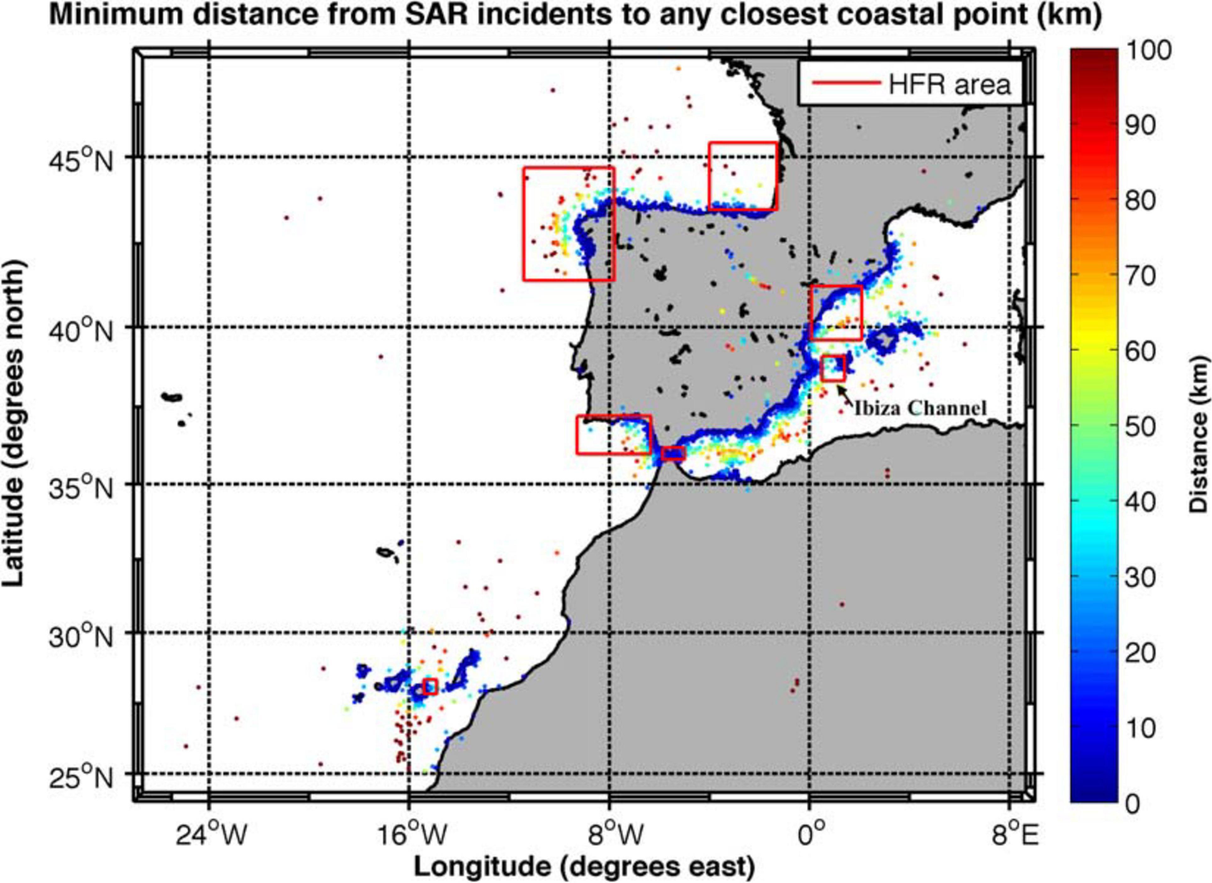
Figure 1. Map covering the four specific SAR areas of responsibility from the Spanish Maritime Search and Rescue Agency showing the location of the SAR incidents from 2019 colored based on their distance to the closest coastal point (as indicated in the color bar). The seven operational HFR systems available within the area are marked with red boxes. Information source: Spanish Maritime Search and Rescue Agency.

At the time of an emergency, SAR operators need to receive information about the reliability of the different ocean model predictions in the most efficient way, to make decisions as quickly as possible. This information should therefore be understandable at first glance. An effective way to display this information could be by means of a model ranking based on the averaged model performance over the area of interest. This can be addressed by computing the spatiotemporal average of SS considering all available drifter observations during a specific period of observations (as in Röhrs et al., 2012; De Dominicis et al., 2014; Roarty et al., 2016; Sotillo et al., 2016; French-McCay et al., 2017; Phillipson and Toumi, 2017; Roarty et al., 2018). However, we show in this article that averages of the SS should be applied and interpreted with caution. Moreover, drifter observations only provide an estimation of the model’s performance along their drifting paths, i.e., over the area and during the time period when they are available. The reliability of this method thus strongly depends on the availability of trajectory observations at the location and at the moment of the incident, or shortly after it (near–real-time evaluation). As this is not always possible because of the scarcity of drifter observations in coastal regions (Tintoré et al., 2019), most of the time there is no alternative but to use the latest observations available in the region, which are not necessarily representative of the dynamics occurring at the moment of the incident. However, in coastal regions, HFR surface currents are now available over wide areas (Figure 1) and provide continuously gridded velocities at the resolution required to tackle small-scale processes. Trajectories derived from HFR could therefore be used to complement drifter observations for evaluating the ocean model predictions in these areas.

In this study, we assess the skill of four ocean forecast systems available in the Ibiza Channel (Western Mediterranean Sea) and evaluate the applicability of the SS in such coastal risk-prone regions seeking for a functional implementation in the context of SAR operations. The surface circulation in this region, mainly driven by local winds (Lana et al., 2016), is highly variable over a wide range of temporal and spatial scales (Robinson et al., 2001; Pinot et al., 2002; Ruiz et al., 2009) and strongly influenced by the intense frontogenesis driven by the confluence of the Liguro-Provençal-Catalan Current and the Atlantic inflow (García-Lafuente et al., 1995; Heslop et al., 2012; Sayol et al., 2013; Hernández-Carrasco et al., 2018a, 2020). We use 22 drifters deployed during three experiments carried out by the Balearic Islands Coastal Observing and forecasting System (SOCIB) and analyze the sensitivity of the SS to different forecast horizons ranging from 6 to 72 h. These experiments were conducted during different seasons, under distinct oceanic conditions, allowing to evaluate the SS sensitivity under diverse dynamical scenarios. Furthermore, we evaluate the validity of applying averages to the SS for comparing the relative average performance of the models, and make recommendations for obtaining an accurate model ranking with this method by introducing the novel SS^∗. Finally, addressing the sparseness of drifter observations that reduces the robustness of the methodology and our capacity to assess the skill of operational systems, we evaluate the use of HFR-derived trajectories for assessing the model performance.

The article is organized as follows. Section “Data and Models” presents the multiplatform observations used for the assessment and the ocean forecast systems evaluated. In section “Model Skill Assessment Methodology,” we provide a description of the methodology developed by Liu and Weisberg (2011) and the skill assessment design applied in this article. The results are presented and discussed in section “Results” and the conclusions are drawn in section “Summary and Discussion.”

Data and Models

Satellite-Tracked Surface Drifters

We use 22 drifters deployed in the Ibiza Channel during three experiments carried out by SOCIB (Tintoré et al., 2013, 2019) in the context of calibration exercises of the HFR system, in September–October 2014 (Tintoré et al., 2014), July–August 2016 (Reyes et al., 2020c), and November–December 2018 (Reyes et al., 2020b) (Figure 2).

FIGURE 2

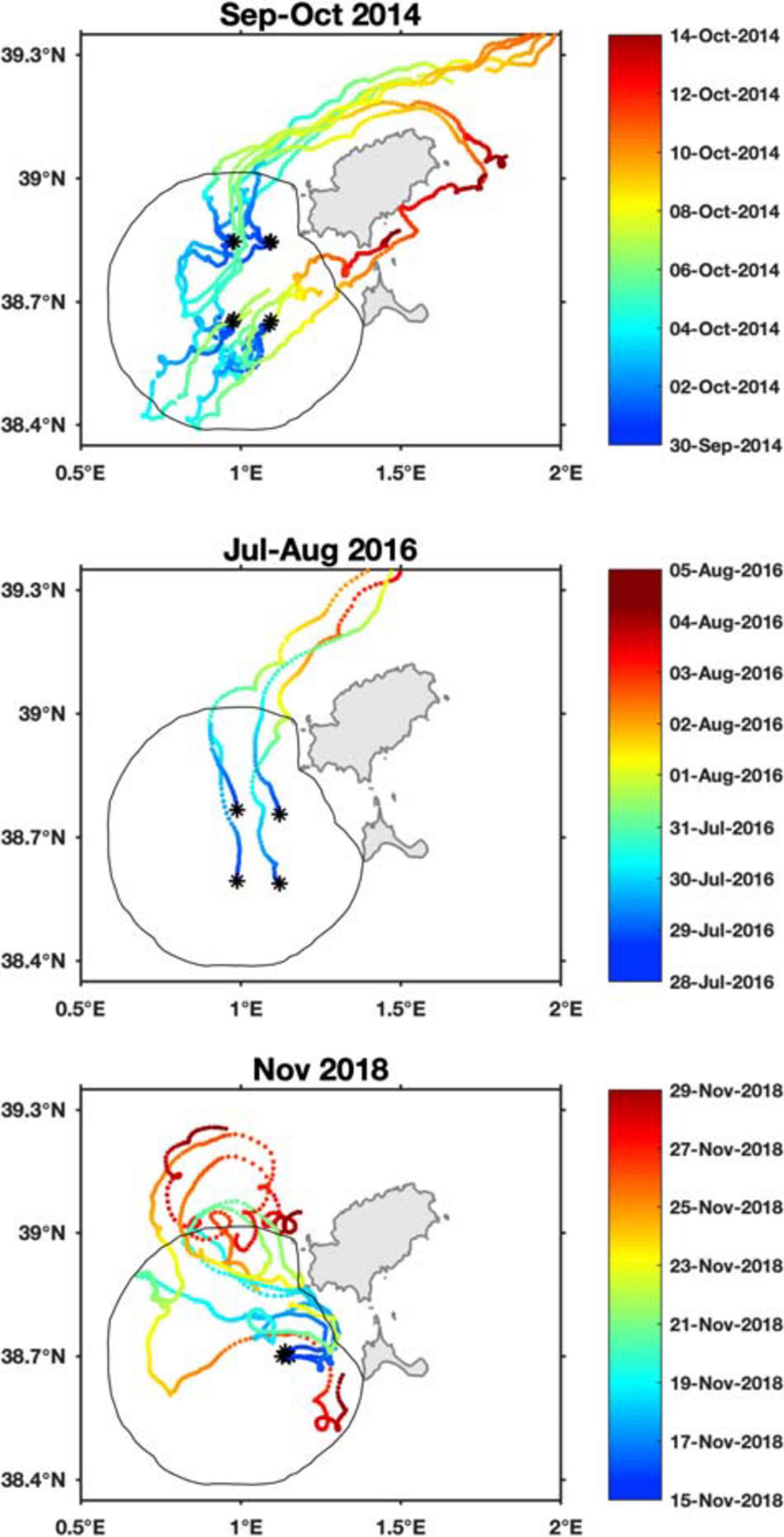
Figure 2. Maps of the trajectories of satellite-tracked drifters available in the Ibiza Channel from the experiments carried out in September–October 2014 (upper panel), July–August 2016 (middle panel), and November 2018 (lower panel). Black stars indicate start locations, and color shows the date associated with drifters’ position, as indicated in the color bar of each panel. The black line shows the contour of the HFR gap-filled surface current coverage.

On September 30, 2014 (Tintoré et al., 2014), 13 drifters were released at four different locations in the Ibiza Channel (Figure 2), as described by Lana et al. (2016). Most of the drifters went northward, trapped by the Balearic current along the northern coast of Ibiza, whereas two drifters went northeastward and crossed the narrow central isthmus between Ibiza and Formentera. Those drifters were of different types (Figure 3): four CODE (cylindrical hull of 10 cm in diameter with a drogue consisting in four sails made of plasticized nylon arranged in a cross-like shape, Davis, 1985), five MDO3i drifters (cylinder of 10 cm in diameter and 32 cm in length, with only 8 cm above the sea surface, with a drogue attached at 0.5-m depth, Callies et al., 2017), and four ODI (spherical hull of 20 cm in diameter and low weight (3 kg), with a drogue of 2 kg attached at 0.5-m depth, Callies et al., 2017). All these configurations ensure that the drifter’s path represents the current within the first meter of the water column, and we indeed do not find clear differences in our results in terms of drifter types (not shown).

FIGURE 3

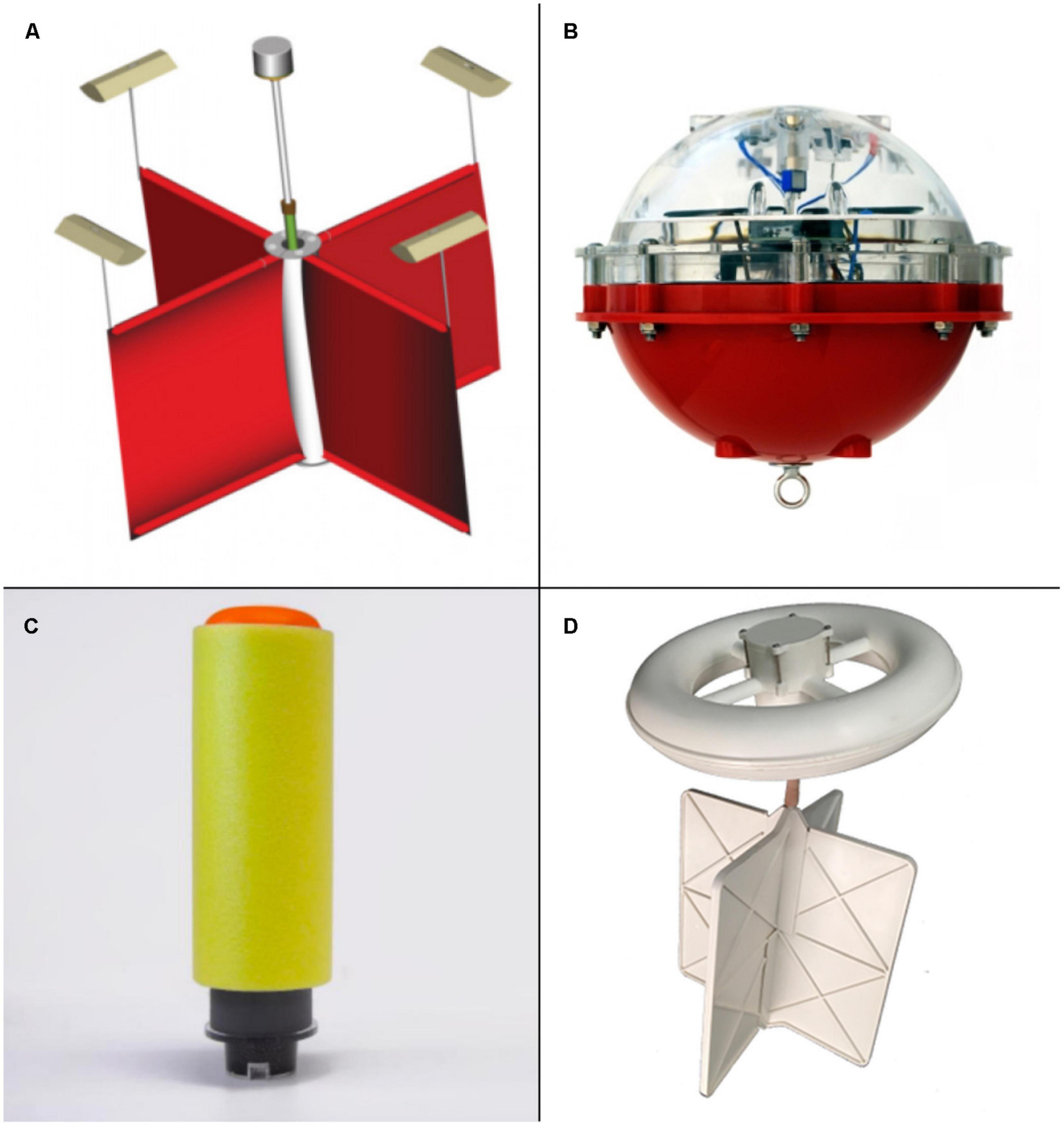
Figure 3. Photographs of the different drifters used in the experiments. (A) CODE (image from the manufacturer Metocean at https://www.metocean.com/product/codedavis-drifter/), (B) ODI from Albatros Marine Technologies (image from the manufacturer at https://issuu.com/eduardvilanova/docs/odi_iridiumoceandriftersolar), (C) MD03i from Albatros Marine Technologies (images from the manufacturer at https://issuu.com/eduardvilanova/docs/minidrifteriridium_md03i), and (D) CARTHE from Pacific Gyre (image from the manufacturer at https://www.pacificgyre.com/carthe-drifter.aspx).

On July 28, 2016 (Reyes et al., 2020c), four ODI drifters were launched at four different locations (Figure 2). That time, all drifters went northward, trapped in the Balearic Current, and got outside the Ibiza Channel in less than 3 days. After 2 days, one of the drifters stopped emitting data (after July 29, 22:00), so we can only consider its trajectory during the first 2 days. Consequently, its trajectory cannot be considered for forecast times longer than 48 h. To ensure a correct comparison of the models at different forecast times of up to 3 days, this drifter is excluded from the sensitivity analysis.

On November 15, 2018 (Reyes et al., 2020b), five CARTHE drifters (Novelli et al., 2017; D’Asaro et al., 2018) were released within a circular area of 2 km in diameter, offshore of Formentera Island (Figure 2). CARTHE-type drifters are biodegradable drifters (Figure 3) and are representative of the upper 0.6 m. In this experiment, the drifters were entrapped in small-scale circulation patterns. During the first week, all drifters followed the same path and went eastward and then northward. Then, two drifters went westward and then took opposite directions, whereas the three other drifters got trapped in eddies in the northern part of the Ibiza Channel.

As the purpose of our article is not to evaluate the Lagrangian model simulation, we do not consider the errors in drifter observations (e.g., O’Donnell et al., 1997). However, quality-control tests have been applied, following the procedure of the SOCIB-Data Centre Facility (Ruiz et al., 2018). CODE drifters provide positions every 10 min, whereas MDO3i and ODI drifters provide positions not evenly distributed in time, every 5–15 min. Linear interpolation is therefore applied to the drifter positions in order to work with equally spaced hourly time series.

In the case of an emergency, SAR operators need to know the accuracy of the model predictions in an area of up to a few kilometers around the location of the incident. Moreover, the ocean being highly variable in both space and time, the evaluation of ocean models needs to be performed over a reduced area and period. For this reason, and to ensure the availability of multiplatform observations, we focus on the region around the Ibiza Channel [0.5°E–2°E; 38.35°N–39.35°N] (Figure 2), where an HFR system is available. Moreover, in 2014 and 2018, we only consider the first 14 days of the experiment, including 88% and 76% of the original dataset, respectively. However, the same conclusions are reached when considering the whole trajectories of the drifters, which extend further north over the Balearic Sea.

High-Frequency Radar System of the Ibiza Channel

High-frequency radar is a shore-based remote-sensed technique that relies on the Bragg resonance phenomenon (Barrick et al., 1977). The HFR of the Ibiza Channel is part of the multiplatform observing system operated by SOCIB (Tintoré et al., 2013, 2019). The HFR system consists of two CODAR SeaSonde radial stations, transmitting at a center frequency of 13.5 MHz with a bandwidth of 90 KHz (Lana et al., 2015, 2016). Hourly radial velocity maps (i.e., velocities toward or away from one antenna) from both stations are combined to form vector surface current velocities on a regular 3 × 3 km grid, with a range of up to 65 km from the shore (Tintoré et al., 2020).

The increased availability of continuous high-resolution HFR surface currents is providing new possibilities for the application of Lagrangian methods to understand small-scale coastal transport processes (Berta et al., 2014; Solabarrieta et al., 2016; Rubio et al., 2017; Hernández-Carrasco et al., 2018b). However, hardware and software failures or environmental conditions can result in incomplete spatial coverage or periods without data. This particularly occurs at the baseline which joins the two stations and at the outer-edge domain, where the Geometrical Dilution of Precision (GDOP) error is higher (Chapman et al., 1997; Barrick, 2006).

With the purpose of obtaining HFR-derived Lagrangian trajectories (see section “Use of HFR-Derived Trajectories”), the generation of HFR gap-filled products are required (Solabarrieta et al., 2016; Hernández-Carrasco et al., 2018a,b). To do this, we use the Open-Boundary Modal Analysis (OMA) method, implemented by Lekien et al. (2004) and further optimized by Kaplan and Lekien (2007), using the modules of the HFR Progs MATLAB package¹. OMA is based on a set of linearly independent velocity modes that are fit to the radial data. These modes (189 in our case) describe all possible current patterns inside a two-dimensional domain (considering the open boundaries and the coastline). OMA considers the kinematic constraints imposed by the coast by setting a zero normal flow. Depending on the constraints of the methodology, it can be limited in representing localized small-scale features, as well as flow structures near open boundaries. Also, difficulties may arise when the horizontal gap size is larger than the minimal resolved length scale (Kaplan and Lekien, 2007) or when only data from one antenna are available, which was not the case during the periods considered here. To avoid the occurrence of unphysically fitted currents, gaps are filled only if they are smaller than the smallest spatial scale of the modes (Kaplan and Lekien, 2007).

Global and Regional Ocean Models

Four ocean forecast systems available operationally in the Ibiza Channel are evaluated: the global model (Lellouche et al., 2018) from the Copernicus Marine Environmental Monitoring Service (CMEMS)², the two CMEMS regional models of the IBI (Iberia-Biscay-Ireland; Sotillo et al., 2015) and MED (Mediterranean) regions (Simoncelli et al., 2014; Clementi et al., 2017), and the regional model of the Western Mediterranean Operational (WMOP) Forecasting System from SOCIB (Juza et al., 2016; Mourre et al., 2018). Table 1 summarizes the main characteristics of these models. They will be referred hereinafter to as GLO, IBI, MED, and WMOP.

TABLE 1

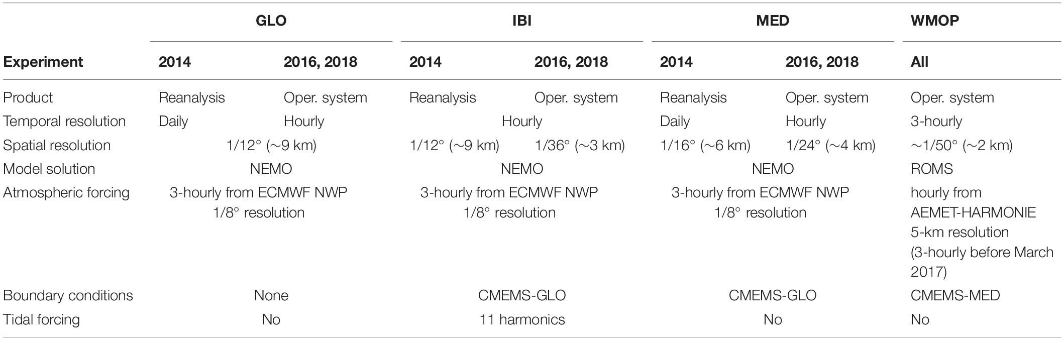
Table 1. Main characteristics of the four Operational Ocean Forecast Systems evaluated.

IBI and MED are nested inside GLO, whereas MED is the parent model of WMOP. CMEMS models are forced with 3-hourly atmospheric fields from the European Center of Medium Weather Forecast (ECMWF) Integrated Forecast System, whereas WMOP was forced for the periods considered in this study by 5-km resolution HIRLAM model atmospheric fields (3-hourly in 2014 and 2016 and hourly in 2018) from the Spanish Meteorological Agency (AEMET). All these systems are run operationally, producing several-day forecasts of a number of physical parameters, including ocean currents. In this article, the historical best estimates of 24-h-forecast horizon are used, except in 2014 when CMEMS forecast estimations were no longer available and their reanalysis is used.

While GLO and MED include data assimilation from satellite altimetry and Argo floats over the whole period of study, IBI and WMOP prediction systems have only implemented data assimilation in March 2018 and November 2018, respectively. The drifter trajectories are not assimilated in any of the models. All models include river runoff, and none of the models includes tidal forcing except IBI, with 11 tidal harmonics (M2, S2, N2, K1, O1, Q1, M4, K2, P1, Mf, and Mm) built from FES2004 (Lyard et al., 2006) and TPXO7.1 (Egbert and Erofeeva, 2002) tidal model solutions.

Model Skill Assessment Methodology

Normalized Cumulative Lagrangian Separation Distance and SS

The Normalized Cumulative Lagrangian Separation (NCLS) distance, developed by Liu and Weisberg (2011), is defined as the cumulative summation of the separation distance between simulated and observed trajectories (i.e., the cumulative separation distance, referred to as D), weighted by the length of the observed trajectory accumulated in time (i.e., the cumulative observed trajectory length, referred to as L), as follows:

$$\text{NCLS}=\frac{D}{L}=\frac{{\sum }_{i=1}^N{d}_i}{{\sum }_{i=1}^{N}l{o}_i}(1)$$

where d_i is the separation distance between observed and simulated trajectories at time step i, lo_i is the length of the observed trajectory at time step i, and N is the forecast horizon. All distances are calculated using the plane sailing formula.

In contrast with the simple separation distance, the NCLS is able to estimate the relative performance of a model in strong and weak current regions. However, as a measure of trajectory model performance, the NCLS is counterintuitive to the conventional model skill scores (e.g., Willmott, 1981; Liu et al., 2009). Indeed, the smaller the NCLS value, the better the model performance. Thus, Liu and Weisberg (2011) proposed a new SS defined as follows:

$$SS=\{\begin{array}{c}\hfill 1-\frac{\text{NCLS}}{n},(\text{NCLS}\le n)\hfill \\ \hfill \mathrm{\hspace{0.25em}0},(\text{NCLS}>n)\hfill \end{array},(2)$$

where n is a nondimensional, positive number that defines the tolerance threshold for no skill. This threshold corresponds to the criterion that the simulation is considered as having no skill (i.e., SS = 0) if the growth of the predictability error is larger than n times the mean flow displacement, i.e., D≥n×L. Larger (smaller) n values correspond to lower (higher) requirements to the model. In general, n is set to 1 (e.g., Röhrs et al., 2012; De Dominicis et al., 2014; Berta et al., 2015; Roarty et al., 2016). However, some studies selected the n value heuristically, in such a way that a small percentage of the SS values are negative and set to zero (e.g., n = 2 in Sotillo et al., 2016).

Hence, the formulation of the SS contains two preliminary defined parameters: the forecast horizon N, and the threshold n. In this study, we address the importance of the proper choice of both parameters, based on a sensitivity analysis.

Design of the Skill Assessment Method

Virtual particles are launched hourly along the successive positions of the observed drifters and for a forecast horizon of N=72 h. Pairs of observed and simulated trajectories are then compared hourly at each time step i=1,2,…N, and the SS is computed as a function of N. To ensure an exact comparison at different forecast times, the exact same temporal length of the observed trajectories is considered for all forecast times (i.e., the observed trajectories minus the last 72 h of observation).

The virtual trajectories are computed using the COSMO Lagrangian model described by Jimeìnez Madrid et al. (2016), which is a free software available in GitHub repository³ (version from June 5, 2019, doi: 10.5281/zenodo.3522268). COSMO consists of a fifth-order Runge-Kutta advection scheme (RK5) with a time step of 1 h, with a bicubic interpolation in space and a third-order Lagrange polynomial interpolation in time, and does not include diffusion, Stokes drift, or beaching. This article focuses on the methodology for comparing the performance of different ocean models in predicting trajectories, but does not focus on the performance of the trajectory model itself. For this reason, we use a very simple trajectory model and do not consider the errors in Lagrangian modeling (e.g., van Sebille et al., 2018). However, it has been verified that the trajectories simulated by COSMO using WMOP currents agreed with the ones simulated using CDrift (Sayol et al., 2014), as shown in Reyes et al. (2020a).

Results

Spatiotemporal Distribution of the SS

We start analyzing the spatiotemporal distribution of the SS of each model considering the case of a high skill model requirement (n=1) and two typical time horizons for model predictions (N=72 h and N=6 h). Figure 4 shows that the SS at 72 h exhibits high spatiotemporal variability, with very different values, depending on the model and the period considered.

FIGURE 4

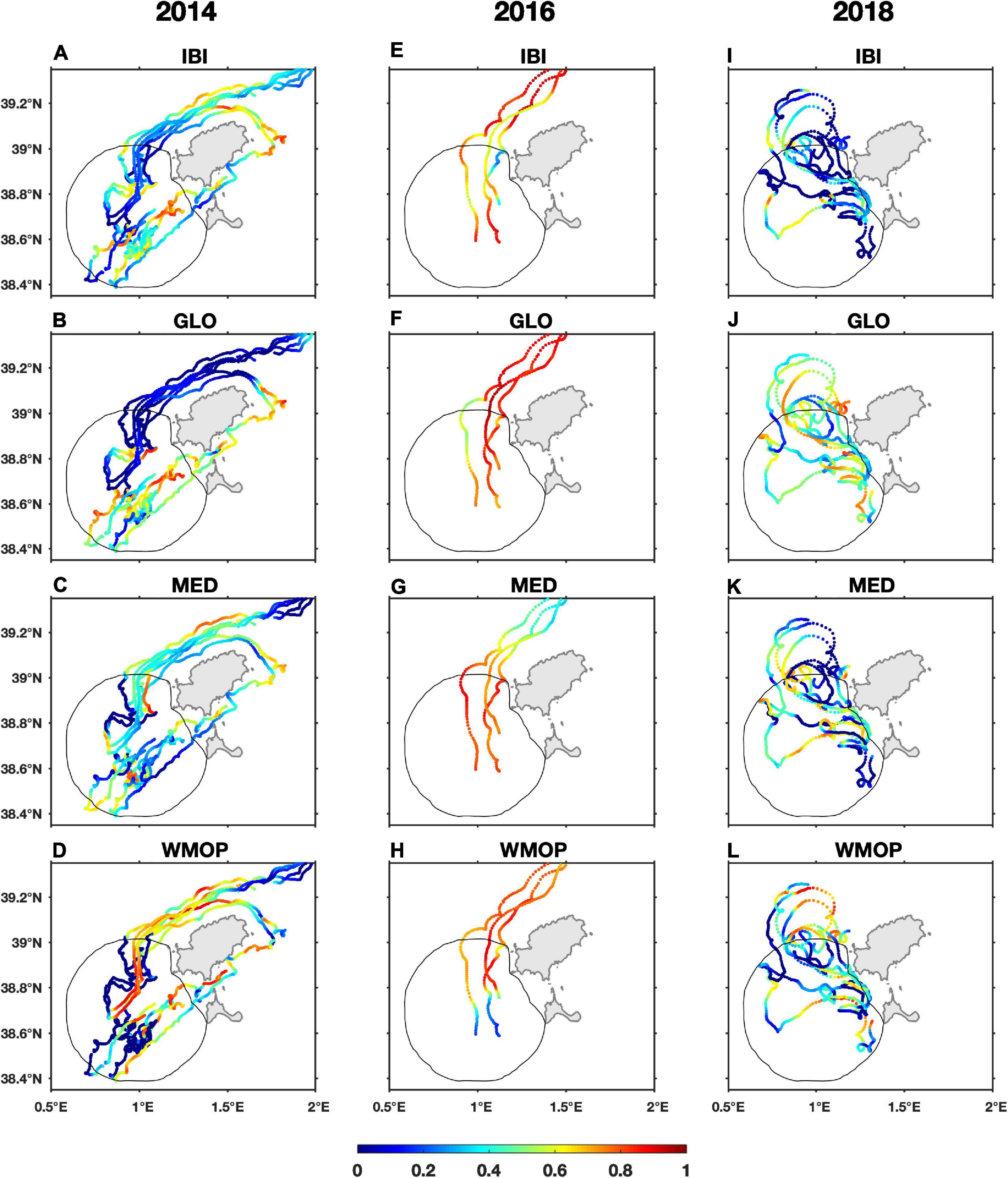
Figure 4. Map of the Ibiza Channel showing the spatiotemporal distribution of the Skill Score obtained for each model as indicated in the figure title, using the drifters of the experiments of 2014 (A–D), 2016 (E–H), and 2018 (I–L) and with a forecast horizon of 72 h. Note that IBI and MED spatial resolution is 1/12° and 1/16° in 2014, in contrast with the 2016 and 2018 experiment when IBI is 1/36° and MED is 1/24°. The black line shows the contour of the HFR gap-filled surface current coverage.

In 2014, WMOP outperforms the other models in the region of strong frontal dynamics along the northern coast of Ibiza (SS > 0.6, Figure 4D). On the contrary, GLO shows no skill in this region (SS∼0, Figure 4B), but obtains the best performance among models in the south of the Ibiza Channel, and shows similar skill to WMOP in the northeastern side of the Ibiza-Formentera Islands (SS∼0.4−0.8, Figures 4B,D). IBI also outperforms its parent-model GLO along the northern coast of Ibiza (Figure 4A), but shows similar or even lower skill elsewhere. In the Ibiza Channel, WMOP shows both instances of low (SS∼0) and very high performance (SS > 0.8, Figure 4D), revealing the high temporal variability of the model predictive capability. Indeed, low SS values are obtained over the positions observed at the beginning of the experiment (September 30 to October 2, 2014; see Figure 2), whereas very high SS values (the best among models) are obtained a few days later, on October 6–8, 2014. We come back to this point in section “The Averaged SS”.

In 2016, all models perform better than in 2014 and 2018, probably because all drifters were entrapped in the density-driven Balearic current (Ruiz et al., 2009; Mason and Pascual, 2013), which is generally better represented in the models. However, spatial differences are also observed: WMOP shows high performance north of 38.8°N (SS > 0.7) but lower performance in the southern part (SS∼0.3, Figure 4H), in agreement with past studies that have shown that WMOP has a larger bias in the southern part of the Ibiza Channel (e.g., Aguiar et al., 2020). On the other hand, MED shows higher performance in the Ibiza Channel (SS > 0.7) than in the northern part (SS∼0.4, Figure 4G). Similarly, GLO exhibits lower SS values in the westernmost part (Figure 4F), and IBI has lower skill in the vicinity of Ibiza (Figure 4E).

In 2018, it is striking that GLO shows the highest SS over the entire region (SS∼0.3−0.7, Figure 4J), despite its lower spatial resolution compared to the other models (Table 1). On the opposite, its child-model IBI shows the lowest performance (SS < 0.4 in most cases, Figure 4I). In some areas, WMOP obtains very high SS [e.g., in the northern part, where drifters got trapped in an eddy (Figure 4L)], being able to improve its parent-model MED (Figure 4K). However, WMOP also obtains lower SS than MED in other regions (e.g., on the westernmost part of the trajectories).

We now compute the SS with a forecast horizon of N=6 h (Figure 5), which is more consistent with the duration of the search that maximizes survivors in SAR missions (US Coast Guard Addendum, 2013). Although the regional differences observed in Figure 4 are still present (e.g., WMOP shows better performance along the northern coast of Ibiza than in the southern part of the Ibiza Channel in both 2014 and 2016, Figures 5D,H), the SS exhibit lower values and more irregular patterns. The case of GLO in 2018 is still striking: whereas GLO clearly exhibits the best performance with a forecast horizon of 72 h (right panels of Figure 4), its performance is much lower at 6-h forecast (Figure 5J vs. Figure 4J), providing only slightly higher SS than the other models (right panels of Figure 5).

FIGURE 5

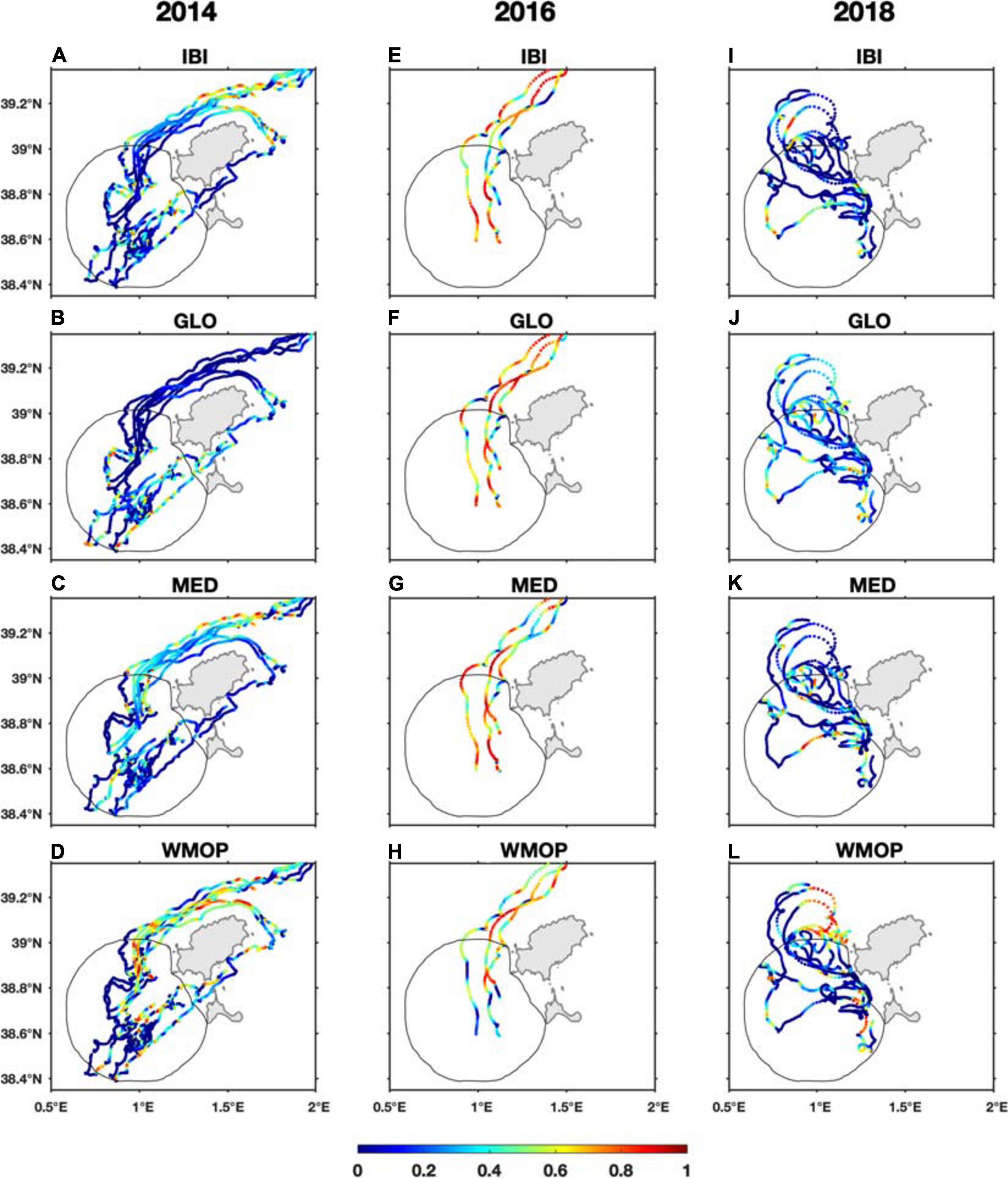
Figure 5. Same as Figure 4, for the experiments of 2014 (A–D), 2016 (E–H), and 2018 (I–L), but with a forecast horizon of 6 h.

Sensitivity to the Forecast Horizon

To further understand the SS dependence on forecast horizon, we analyze the cumulative separation distance D, the cumulative observed trajectory length L, the NCLS, and the SS obtained along each drifter path, for each model, and for different forecast horizons N. Since GLO in 2018 exhibits a striking rise of the SS, we show in Figure 6 this analysis for GLO along the path of one drifter in 2018. However, similar results are obtained for all drifters and all models (not shown).

FIGURE 6

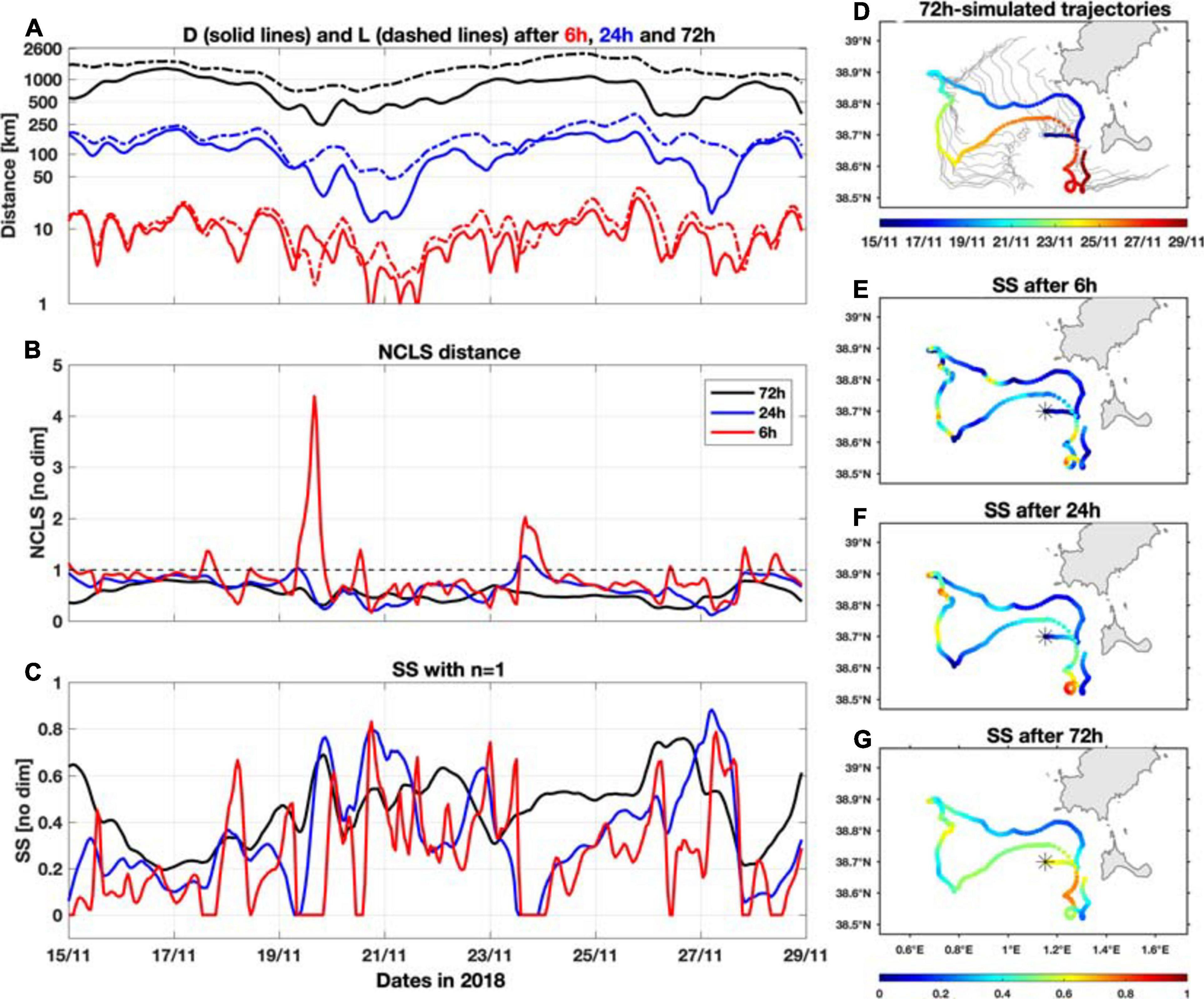
Figure 6. Temporal evolution of the (A) cumulative separation distance D between simulated and observed trajectories (solid lines) and the cumulative observed trajectory length L (dashed lines) (in logarithmic scale), (B) NCLS distance and (C) SS obtained using n=1 for the model GLO along the path of a drifter during the 2018 experiment, after 6 h (red lines), 24 h (blue lines), and 72 h (black lines) of simulation. The black dashed line in the b-panel shows the threshold n=1. (D) Maps of the 72 h–simulated trajectories (gray lines) released at hourly positions (for better clarity, trajectories are plotted only every 6 h) along the drifter trajectory represented by color dots showing the date associated with drifters’ position. (E–G) Spatiotemporal distribution of the SS obtained along the drifter path after (E) 6, (F) 24, and (G) 72 h of simulation. Black asterisks indicate start location.

As observed in Figure 6A, L is, on average, always larger than D, and L grows with advection time at a much higher rate than D: whereas they are of the same order of magnitude after 6 h of simulation (D ranges from 0.7 to 26 km with a mean value of 8.8 km, and L ranges from 1.7 to 35 km with a mean value of 11.3 km), L is almost twice D after 72 h of advection (D ranges from 245 to 1403 km with a mean value of 753 km, whereas L ranges from 694 to 2,220 km, with a mean value of 1,372 km). In other words, the cumulative absolute dispersion of the observed drifter grows much faster than the cumulative separation distance.

Figure 6B shows the evolution of the NCLS distance (Eq. 1). At 6-h forecast, the NCLS shows spikes, which are much less pronounced after 24-h forecast, and nonexistent after 72 h. Those spikes, as already noted by Liu and Weisberg (2011) for a 1-day simulation, are due to the sudden decrease of the trajectory length L compared to the cumulative separation distance D (Figure 6A). Particularly, they are related to small-scale dynamical features that induce slow currents and consequently a small displacement of the observed drifter and that are not well represented by the models, such as inertial oscillations. However, removing the inertial oscillations applying a 40-h low-pass filter leads to even smaller values of L and consequently more occurrences of NCLS spikes (not shown). As L becomes much higher than D as the forecast time increases, there are more situations of significantly large NCLS values at shorter forecast time than at longer forecast time (Figure 6B). Considering n=1, SS=0 if NCLS > 1. As the NCLS spikes are higher and more frequent at shorter forecast times, the SS get more zero values and is thus more irregular after 6-h forecast than after 24 or 72 h (Figure 6C).

Another observation from Figure 6B is the decrease of the NCLS distance with forecast time in most cases, dropping from an average of 0.84 at N=6 h to 0.55 at N=72 h, resulting in the increase of the SS (Figures 6C,E,F,G), rising from an average of 0.25 at N=6 h to 0.45 at N=72 h. This tendency is directly related to the higher rate of L with respect to D, as seen before (Figure 6A), and can result from two different scenarios. First, this can result from the convergence of the simulated and observed trajectories as the forecast time increases, inducing a decrease of the separation distance. For instance, during the first days of the experiment, GLO simulates northwestward trajectories, whereas the observed drifter goes eastward then northward and then westward (Figure 6D). The simulated trajectories launched during the first hours of the experiment thus finally converge with the observed drifter path after a certain time. As a result, the SS increases from SS∼0.1 at 6-h forecast to SS∼0.5 at 72-h forecast.

Second, the higher rate of L with respect to D can result from rapidly evolving local structures such as small-scale eddies that induce a large displacement of the observed drifter. As an example, we show in Figure 7A a drifter trajectory between November 25, 2018, 19:00 and November 28, 2018, 19:00, and the corresponding simulations from the four models. While GLO performs the best during the first 12 h and thus obtains the highest SS (Figure 7D), its simulated trajectory deviates from the observed one during the following hours. However, its SS increases from SS∼0.4 at 12-h forecast to SS∼0.6 after 72 h because the distance traveled by the drifter strongly increases when the drifter becomes entrapped in a highly energetic structure, whereas the separation distance increases only slightly (Figures 7A–C). Similarly, MED and IBI exhibit an increase of the SS with forecast time (Figure 7D), although their simulated trajectories go in the opposite direction than the observed one (Figure 7A). On the other hand, the SS of WMOP increases with forecast time because the resemblance between the simulated and observed trajectories is better after the first 6 h of simulation. This example illustrates the high dependence of the SS model ranking to the forecast horizon: whereas the SS of GLO is the highest among models for a simulation time < 24 h, WMOP and GLO obtain a similar value of SS∼0.6 from 36 h of simulation (Figure 7D).

FIGURE 7

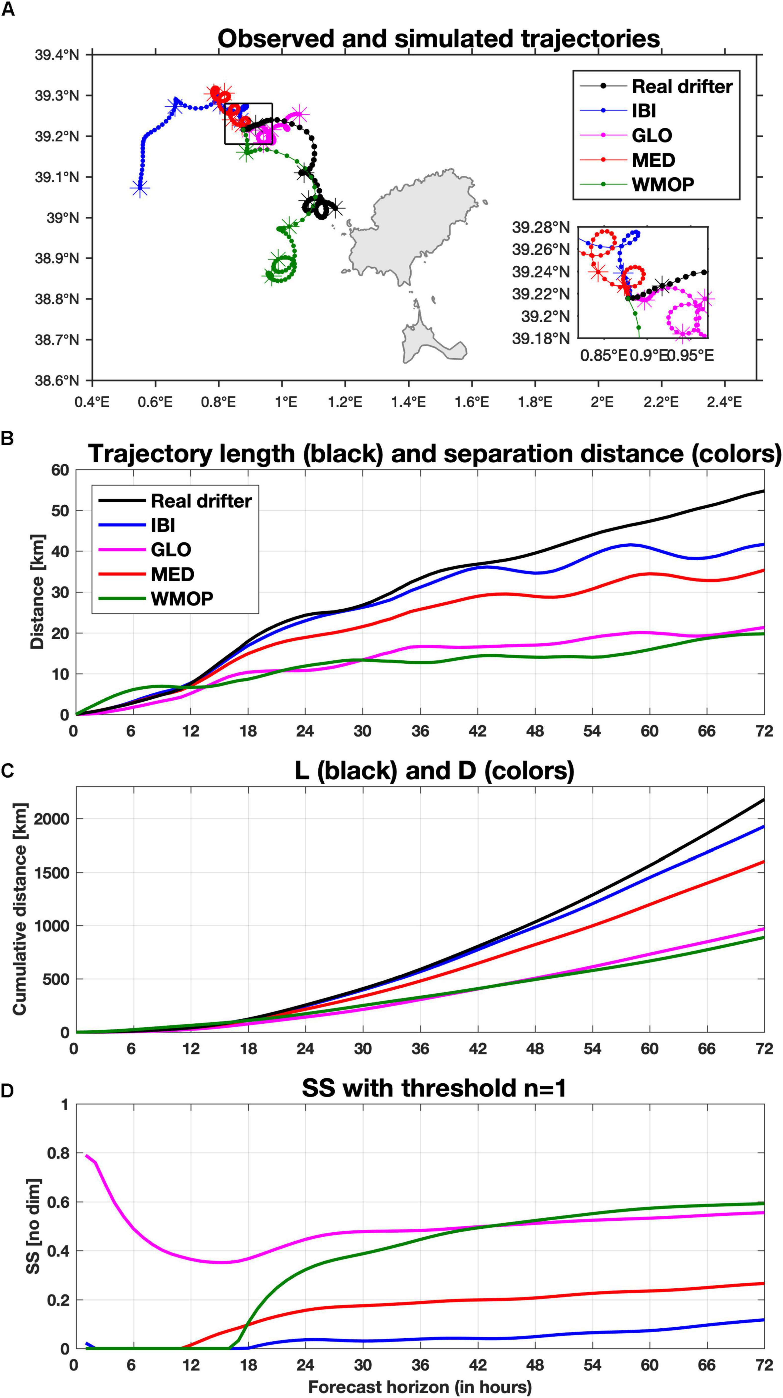
Figure 7. (A) Observed trajectory (black dotted line) of a drifter from November 26, 2018, at 00:00 to November 29, 2018, at 00:00 and simulated trajectories launched at the initial position and calculated with IBI (blue), GLO (magenta), MED (red), and WMOP (green). Positions after 6, 24, 48, and 72 h of forecast are indicated by asterisks. Lower panels: temporal evolution along the forecast horizon, in hours, of the (B) separation distance between observed and virtual trajectories (colored lines) and observed trajectory length (black line), (C) cumulative separation distance D (colored lines) and cumulative observed trajectory length L (black line) and (D) Skill Score as defined by Liu and Weisberg (2011) obtained for each model using a threshold n = 1.

The SS is therefore strongly dependent on the forecast horizon, and an overly long forecast time can lead to an overestimation of the SS. Hence, although a short forecast time leads to more irregular SS patterns because of not well-resolved small-scale dynamics, in coastal areas characterized by high variability of the surface currents, a short forecast time should be applied (e.g., 6 h). In the rest of this article, we therefore consider a forecast horizon of 6 h.

The Averaged SS

We now examine the best way to obtain a model ranking based on the spatiotemporal average of SS considering the whole period of observations. However, in the definition of the SS, the negative values are imposed to zero. The average of SS thus overestimates the averaged model’s skill and can be misleading. In fact, the negative values indicate how far is the NCLS to the tolerance threshold n and thus give information on how far the simulated trajectory is from the observation. These values should therefore be included in the calculation.

For each experiment and each model, Figure 8 shows the histogram of SS^∗, which is defined as the SS, but without the imposition of the negative values to zero, such as:

FIGURE 8

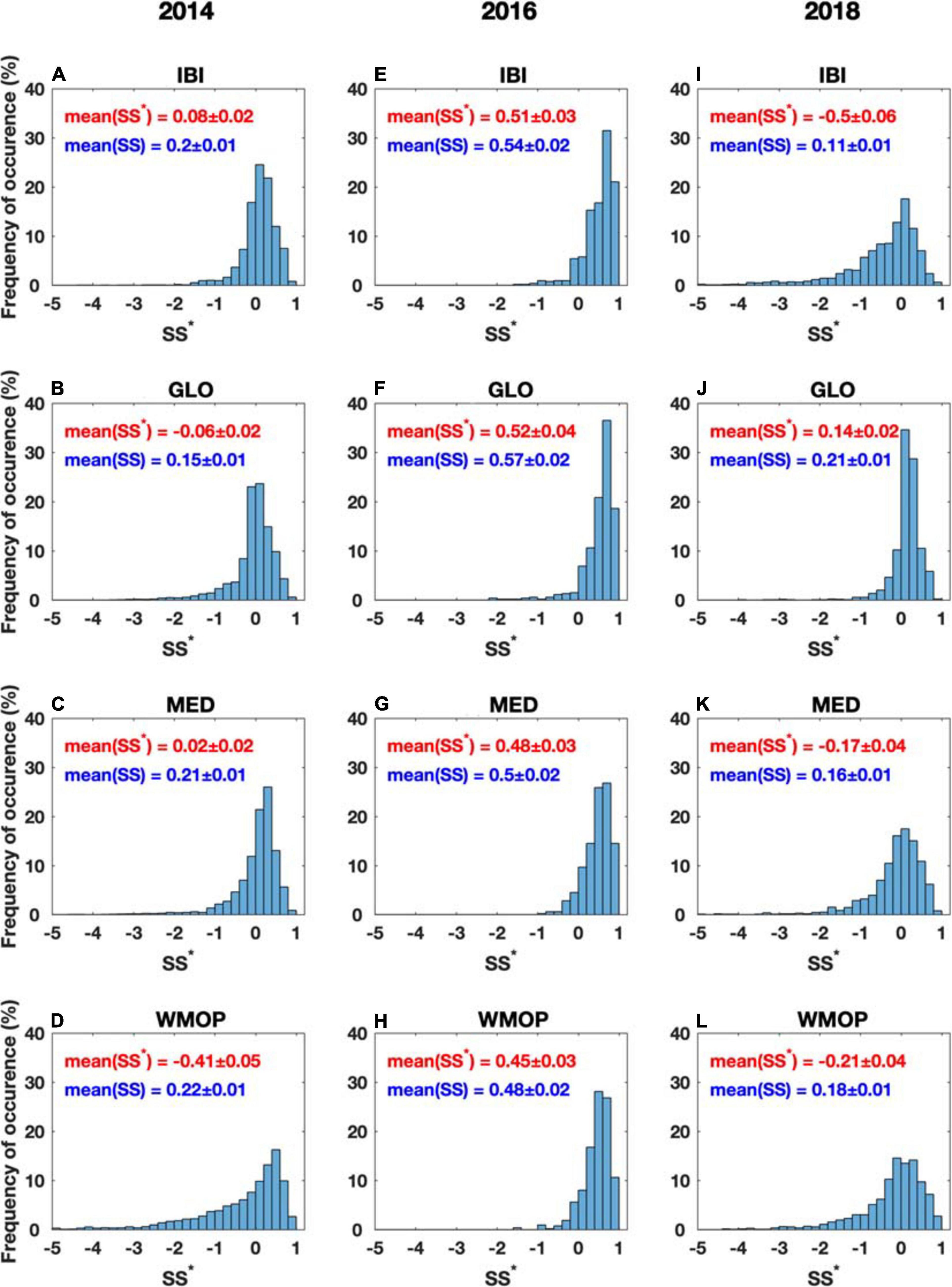
Figure 8. Histogram of the values of the Skill Score SS* (defined by Eq. 3) in the range [−5, 1] with bins of 0.2, obtained for IBI, GLO, MED, and WMOP (top-to-bottom panels) using the drifters of 2014 (A–D), 2016 (E–H), and 2018 experiment (I–L) after a simulation of 6 h. The averaged SS (as defined by Liu and Weisberg, 2011) and the averaged SS* are given in blue and red, respectively.

$$S{S}^{*}=1-\frac{\text{NCLS}}{n},\forall \mathrm{NCLS}\in [0\mathrm{\infty }].(3)$$

As in the previous section, we use n=1. The average $\overline{SS}$ and the average $\overline{S{S}^{*}}$ are given in Figure 8 in blue and red, respectively, together with their confidence intervals. These confidence intervals have been estimated in two ways, providing similar results. The first approach uses the bootstrap distribution of $\overline{S{S}^{*}}$ from 10,000 resamples, whereas the second method is based on the Student t distribution.

In 2014, the SS^∗ of IBI, GLO, and MED exhibit a nearly bell-shaped distribution with a maximum occurrence of near-zero values (Figures 8A–C). The average is therefore close to zero, sometimes even negative, as for GLO ($\overline{S{S}^{*}}=-0.06\pm 0.02$). On the other hand, WMOP obtains a left-skewed distribution, with a higher percentage of values in the range of [0.6–1] compared to the other models, but also more occurrences of large negative values (SS^∗ < −1). Consequently, WMOP obtains the lowest averaged SS^∗ with a negative value of $\overline{S{S}^{*}}=-0.41\pm 0.05$, strongly penalized by large negative values obtained during the first days of the experiment, whereas it obtains the highest performance a few days later, as seen previously in Figure 5D.

In 2016, differences between $\overline{S{S}^{*}}$ and $\overline{SS}$ are much smaller because all models perform better during this period, as already seen in Figure 5, and only a few negative values are obtained (middle panels of Figure 8). Both calculations indicate GLO as the best model on average, although the $\overline{S{S}^{*}}$ differences between GLO, IBI, and MED are not statistically significant at the 95% confidence level. In 2018, on the other hand, $\overline{S{S}^{*}}$ and $\overline{SS}$ are strongly different. GLO is again significantly better than the other models, obtaining a positive averaged score of $\overline{S{S}^{*}}=0.14\pm 0.02$, whereas the other models obtain negative averaged SS^∗ (right panels of Figure 8).

These results show that the imposition of a lower limit value of zero for SS < 0 is not adequate if spatiotemporal averages are computed afterward, as it would lead to a strong overestimation of the averaged SS and could lead to an erroneous model ranking. However, in the context of SAR operations, the SS^∗ could be less intuitive than the SS as it is in the range of [−∞ 1]. A solution could therefore be to determine the appropriate threshold n such that 100% of the SS^∗ values are positive, obtaining a user-friendly metric from 0 to 1. Figure 9 shows the percentage of positive SS^∗ values obtained by each model as a function of n in the range [0.5–3]. As observed, the minimum value of n from which 100% of positive values are obtained differs for each model and experiment. While in 2016, a threshold of n=2 is sufficient, in 2014 and 2018 a tolerance threshold of n > 3 would be necessary.

FIGURE 9

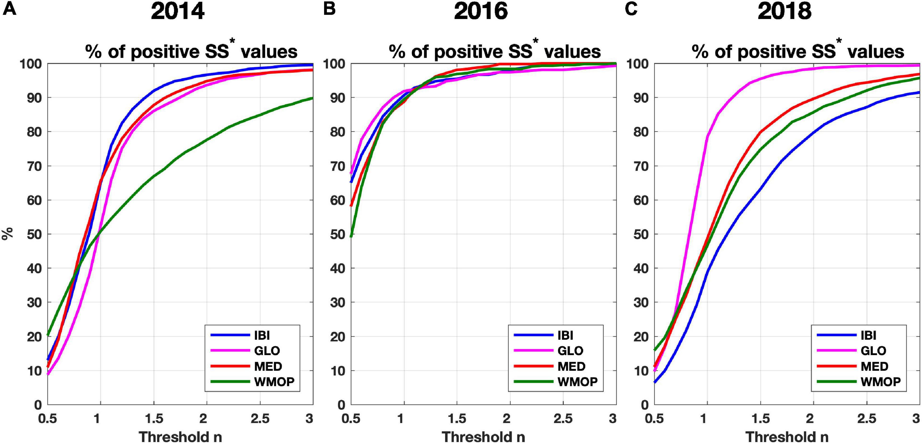
Figure 9. Variation of the percentage of positive SS* values after 6 h of forecast in function of the threshold n in the range [0.5–3] for the experiment of 2014 (A), 2016 (B), and 2018 (C).

This scenario dependence of the appropriate threshold n makes difficult its use in operational applications, where different models have to be simultaneously evaluated in a systematic routine manner. The use of $\overline{S{S}^{*}}$ with n=1 remains therefore the safest solution. The percentage of positive values is an interesting additional metric to provide, as in Phillipson and Toumi (2017), as it is also an indicator of the level of performance. For example, it is striking that in 2014 and 2018, WMOP obtains the highest percentage of positive values among models if a tolerance threshold of n=0.5 is selected, meaning that WMOP obtains the highest percentage of cases where $D<\frac{L}{2}$, although it obtains the lowest score on average in 2014, and the second lowest score in 2018. This again reflects the high variability of WMOP performance, which can be in strong disagreement with the drifters, but also in very good agreement, in this case outperforming the other models.

Use of HFR-Derived Trajectories

We now analyze the use of HFR-derived trajectories to evaluate the model performance. First, we evaluate the skill of HFR in reproducing the drifter trajectories (Figure 10), and compare the $\overline{S{S}^{*}}$ of HFR with the one from the models (Table 2), considering only the drifter observations available inside the HFR coverage. As shown in Figure 2, this corresponds to the period of September 30, 2014, to October 10, 2014 (10 days); July 28, 2016, to July 31, 2016 (4 days); and November 15, 2018, to November 30, 2018 (15 days).

FIGURE 10

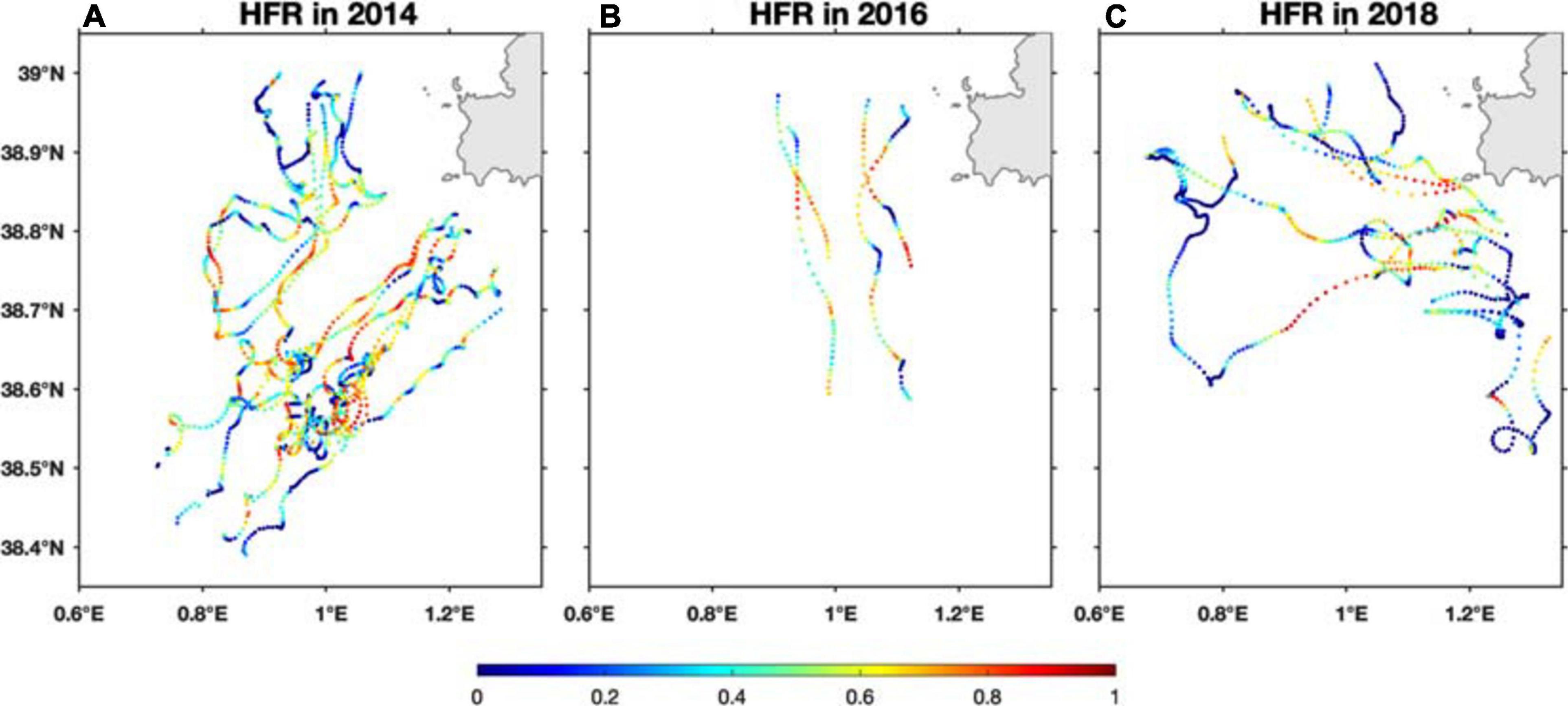
Figure 10. Map of the Ibiza Channel showing the spatiotemporal distribution of the SS obtained for the HFR using all the drifters of the experiments of 2014 (A), 2016 (B), and 2018 (C) inside the HFR gap-filled surface current coverage area, and with a forecast time of 6 h.

TABLE 2

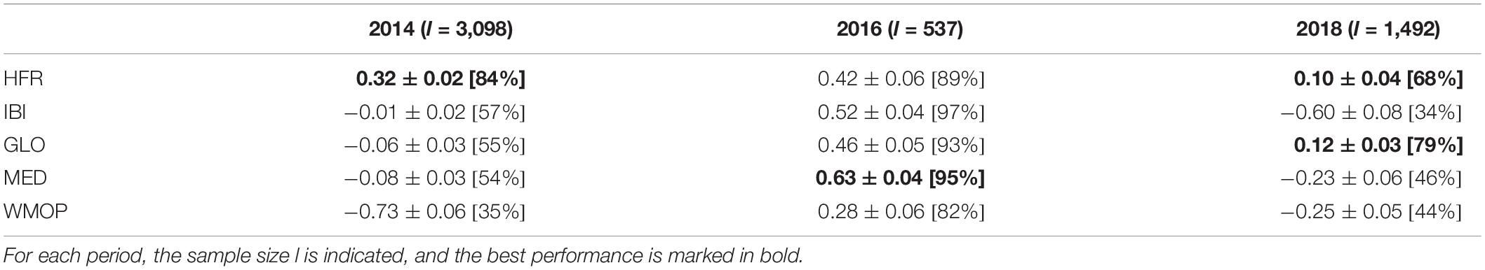
Table 2. Spatiotemporal average $\overline{S{S}^{*}}$ and their confidence intervals obtained after a forecast of 6 h over all the trajectories inside the HFR coverage of the Ibiza Channel.

In 2014, HFR shows much higher skill than models, with $\overline{S{S}^{*}}=0.32\pm 0.02$ and 84% of positive values, whereas the best model, IBI in this case, obtains $\overline{S{S}^{*}}=-0.01\pm 0.02$ with 57% of positive values. In 2016, on the other hand, MED significantly outperforms HFR ($\overline{S{S}^{*}}=0.63\pm 0.04$ and $\overline{S{S}^{*}}=0.42\pm 0.06$, respectively), and GLO and IBI also exhibit higher performance than HFR on average, although the confidence intervals slightly overlap. In 2018, GLO shows similar skill than HFR ($\overline{S{S}^{*}}=0.12\pm 0.03$ and $\overline{S{S}^{*}}=0.10\pm 0.04,$ respectively), but GLO obtains more positive values (79% against 68%). This indicates that models show sometimes better skill than HFR in reproducing the drifter observations, as already noted in Roarty et al. (2016). However, in 2018, the spatiotemporal distribution of the SS^∗ reveals that HFR performs better than any of the models in the center of the domain (Figure 10C vs. the right panels of Figure 5), but shows very low performance in the outer edges, where uncertainties in HFR data are higher because of larger GDOP errors (Chapman et al., 1997) and where data gaps usually occur.

Despite this limitation, HFR allows obtaining a larger number of trajectories, improving not only the robustness of the SS statistics but also the spatial and temporal assessment of the model performance. From now on, we therefore use HFR-derived trajectories to evaluate the models (Figure 11). The methodology consists in selecting the HFR grid points where there is 80% of data availability during the period considered (as recommended by Roarty et al., 2012). We obtain 287 points in 2014, 338 in 2016, and 277 in 2018. Virtual particles are launched hourly from these grid points for a 6-h horizon forecast, and the trajectories simulated by the models are compared against the HFR-derived trajectories. In order not to mix different dynamics, we apply this method during a short time frame of 6 h. As an example, and for comparison with the results obtained using the drifters, we select the first 6 h of the experiments, i.e., from 13:00 to 19:00 on September 30, 2014, and from 13:00 to 19:00 on November 15, 2018. In 2016, this period corresponds to an exercise at the radial sites, and the transmission was off for 4–5 h, decreasing the data availability. We therefore choose the period just after the exercise: from 00:00 to 06:00 on July 29, 2016. However, we reach similar conclusions when computing the SS^∗ hourly during the first 3 days of observations instead of the first 6 h (not shown).

FIGURE 11

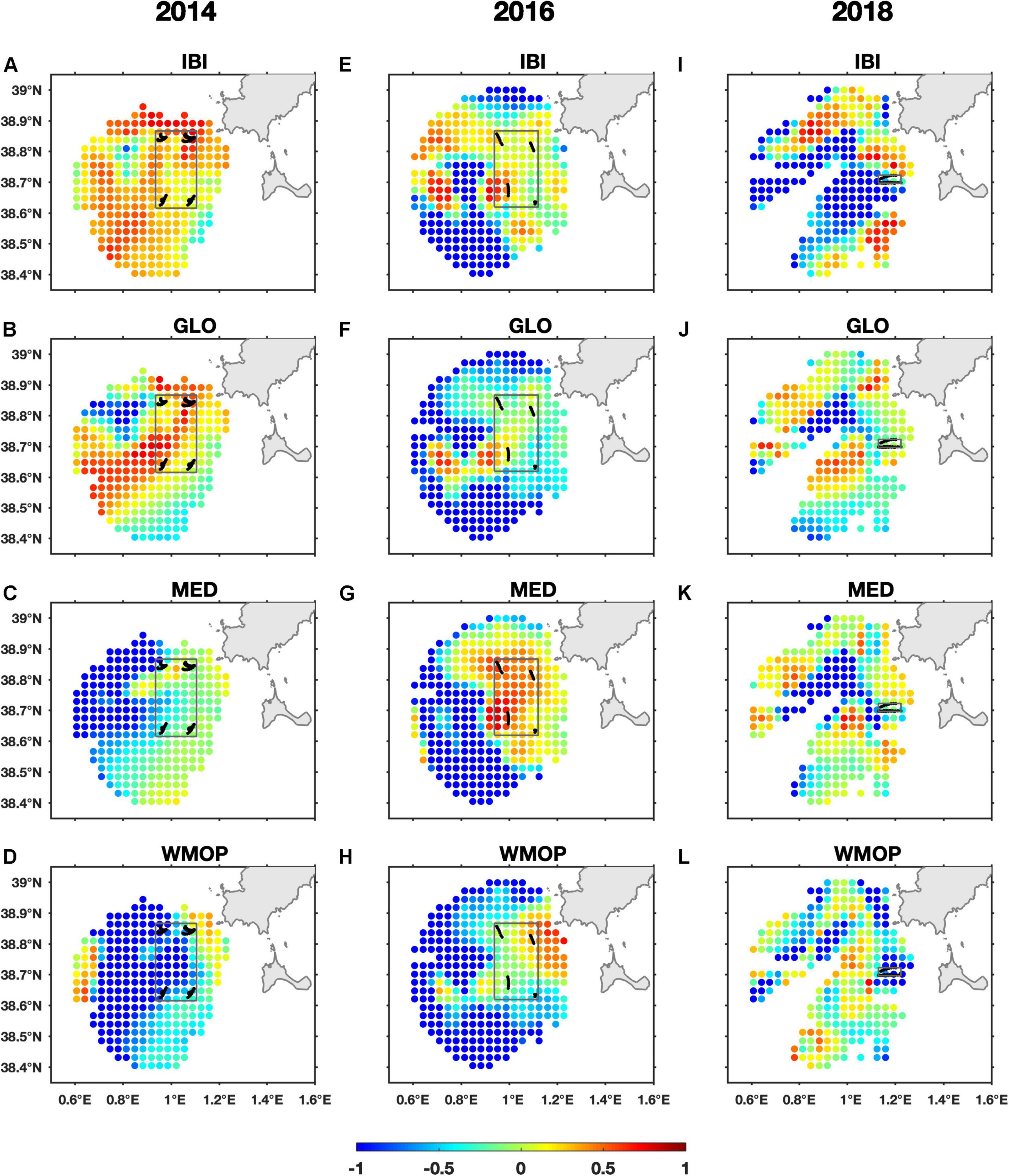
Figure 11. Temporally averaged SS^∗ obtained for each model as indicated in the figure title by comparing against the HFR-derived trajectories during a forecast horizon of 6 h. Simulated trajectories are initialized hourly at each grid points on September 30, 2014, from 13:00 to 19:00 (A–D); on July 29, 2016, from 00:00 to 06:00 (E–H); and on November 15, 2018, from 13:00 to 19:00 (I–L). Black lines show the drifter paths available during the same periods, and the boxes indicate the regions where the averages of Table 3 are applied. The box covers the region [0.9354°E–1.1060°E, 38.6152°N–38.8662°N] in 2014, [0.9384°E–1.1208°E, 38.6189°N–38.8666°N] in 2016; and [1.1297°E–1.2234°E; 38.6962°N–38.7223°N] in 2018. SS^∗ values are only obtained in those grid points with data temporal availability equal to or higher than 80%.

Figure 11 shows the spatial distribution of the temporally averaged SS^∗of each model during these 6-h periods. We use a tolerance threshold of n=1, and a lot of values obtained are negative. In order to not conceal the negative values and observe the spatial variability, the color bar is adjusted to [−1 1]. To ease interpretation, the corresponding averaged surface currents during the same periods from the different models and HFR are shown in Figure 12.

FIGURE 12

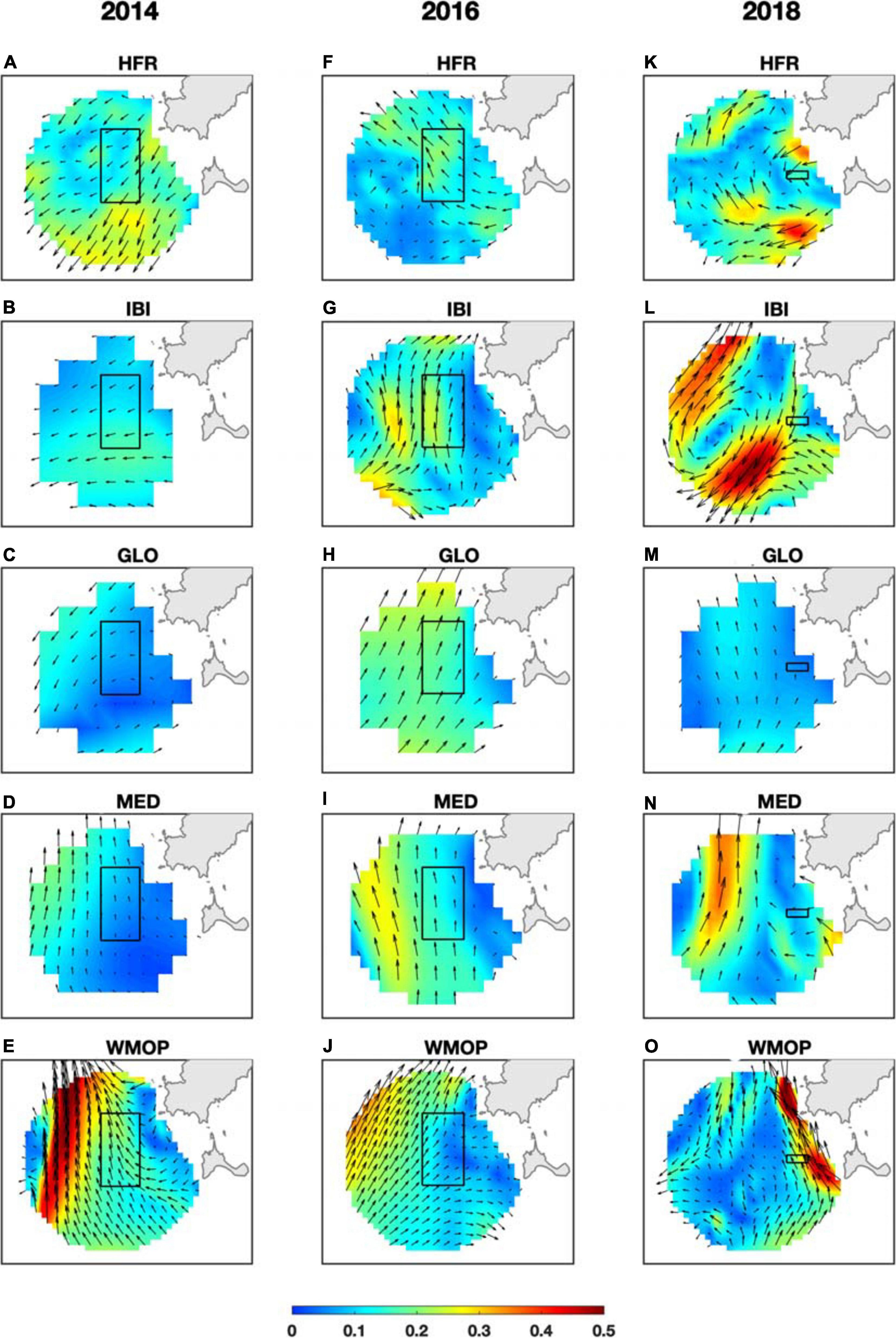
Figure 12. Temporally averaged surface current for each model and HFR OMA surface currents during the first 6 h of the experiments, i.e., on September 30, 2014, from 13:00 to 19:00 (A–E), on July 29, 2016, from 00:00 to 06:00 (F–J), and on November 15, 2018, from 13:00 to 19:00 (K–O). The boxes are the same as in Figure 11 and indicate the regions where the averages of Table 3 are applied.

In 2014, IBI shows the best performance (Figure 11A), being able to improve its parent-model GLO (Figure 11B), with SS^∗ values around 0.5 in most of the domain, in agreement with the relatively good correspondence between IBI surface currents and HFR observations (Figures 12A,B). On the other hand, MED and its child-model WMOP simulate a northward circulation (Figures 12D,E) and show therefore a strong disagreement, especially in the western part, indicated by very low score values (SS^∗ < −1, Figures 11C,D). Interestingly, SS^∗ values are higher (albeit close to zero) in the southeastern part, because the models’ current amplitudes are much weaker (Figures 12D,E), thus leading to smaller separation distances, even though the model outputs do not match with HFR observations.

In 2016, MED shows the best performance in the central and eastern part of the domain (SS^∗∼0.6, Figure 11G). The other models all show lower skills in this region because their surface currents overestimate the eastward component (middle panels of Figure 12). In the western part, IBI exhibits the highest scores (SS^∗∼0.5), while along the island of Ibiza, WMOP shows the greatest resemblance with HFR.

In 2018, IBI shows the best agreement with HFR in the northern and southeastern parts (SS^∗∼0.5, Figures 11I, 12K,L). It is striking that, over the whole domain, GLO obtains globally the best scores, albeit with low SS^∗ values (Figure 11J), whereas its surface currents do not resolve the small-scale features observed by HFR (Figures 12K,M). This is because GLO surface current intensity is much smaller compared to the other models, leading to the shortest separation distances between GLO and HFR trajectories, whereas the higher-resolution models exhibit very energetic circulation features (Figures 12L,N,O), leading to larger separation distances if the structures are not correctly located. However, although these SS^∗ values are the best among models, they are still low (SS^∗0.1) and therefore do not reflect a good agreement between GLO and HFR.

To compare these results with the ones obtained using drifters, we compute the spatial average of the SS^∗ over the areas covered by drifter observations during these 6-h periods (Table 3). As the trajectories cover different regions in each experiment, the areas selected do not cover the same region nor have the same size in the three experiments (Figures 11, 12). In 2018, the area selected is small because all drifters cover the same region during the period considered, whereas in 2014 and 2016, the trajectories are far away from each other. However, as the dynamics is quite consistent over the region (Figure 12), the area covering all trajectories is selected. Furthermore, similar results are obtained if smaller regions are selected (not shown).

TABLE 3

Table 3. Spatiotemporal average $\overline{S{S}^{*}}$ and their confidence intervals obtained after a forecast of 6 h during the first 6 h of experiment and over the boxes indicated in Figures 11, 12, using real drifters and HFR-derived trajectories.

In all experiments, the same model ranking is obtained as when using the drifter trajectories (Table 3). In 2014, GLO outperforms the other models in the region selected, with $\overline{S{S}^{*}}=0.21\pm 0.10$ and $\overline{S{S}^{*}}=0.34\pm 0.05$ obtained from drifter and HFR, respectively. However, GLO and IBI skills are not statistically different, in agreement with their very similar surface currents in this area (Figures 12B,C). In 2016, MED obtains the highest score over the region, with $\overline{S{S}^{*}}=0.55\pm 0.16$ and $\overline{S{S}^{*}}=0.46\pm 0.04$ obtained from drifter and HFR, respectively. In 2018, GLO performs the best with $\overline{S{S}^{*}}=0.01\pm 0.02$ and $\overline{S{S}^{*}}=-0.06\pm 0.01$ obtained from drifter and HFR, respectively. However, as seen previously, these values are low, in agreement with the strong difference between GLO and HFR surface currents in the area, in nearly opposite directions (Figures 12K,M). None of the models is able to adequately represent the ocean dynamics of the area during this period.

Summary and Discussion

We have assessed the Lagrangian performance of four ocean models in the Ibiza Channel applying the methodology developed by Liu and Weisberg (2011) and using 22 drifter trajectories from three different periods under diverse dynamical conditions. The sensitivity of the SS has been analyzed for different forecast horizons ranging from 6 to 72 h, further examining the best way to obtain an average model performance, avoiding biased conclusions, thus introducing the novel SS^∗. Finally, we have evaluated the skill of the HFR surface currents in reproducing the drifter trajectories and analyzed the use of HFR-derived trajectories for assessing the relative performance of the models.

Our analysis shows (see sections “Spatiotemporal Distribution of the SS” and “Sensitivity to the Forecast Horizon”) that the model performance is highly scenario-dependent and can exhibit highly variable SS values over the same region if the available trajectory observations sample different periods dominated by diverse dynamical conditions. This highlights the need of developing skill assessment methods to quantify the models’ performance in a systematic routine manner. We have also shown that the SS is very sensitive to the forecast length, so the forecast horizon should be chosen with caution. At short forecast times (i.e., 6 h), the SS exhibits a much higher variability, with more occurrence of zero values. This is due to the relatively short trajectory lengths L observed compared to the separation distance D obtained at short temporal and spatial scales not properly resolved by the models. Indeed, for short forecast horizons, L can frequently be much smaller than D in case of small-scale dynamical features that induce slow currents and consequently a small displacement of the observed drifter and that are not well represented by the models, such as inertial oscillations. However, removing the inertial oscillations applying a 40-h low-pass filter leads to even smaller values of L and consequently a higher variability of the SS (not shown).

We have also shown that the SS increases with forecast time in most cases (see section “Sensitivity to the Forecast Horizon”) because the cumulative length of the observed drifter grows faster than the cumulative separation distance (i.e., L≫D), without necessarily implying a good model performance. This tendency is explained, on the one hand, to the decrease of the separation distance with time due to high variability of the surface currents that lead to the convergence of the simulated and observed trajectories after a certain time and, on the other hand, by the strong increase of trajectory length L in case of intense small-scale dynamics, which occur very often in coastal areas. An overly long forecast time thus leads to an overestimation of the SS. Hence, in coastal areas characterized by high variability of the surface currents, a short forecast time should be applied (e.g., 6 h), although it leads to more irregular SS patterns.

For SAR operation purposes, we examined the best way to identify the model with the highest mean performance over an area and along a specified period (see section “The Averaged SS”). We have shown that the averaged SS can be misleading because of the previous imposition of the negative values to zero (Eq. 2). Indeed, whereas the original definition of the SS is correct for analyzing its spatiotemporal distribution (as in section “Spatiotemporal Distribution of the SS”), it is not adequate if averages are going to be applied afterward, especially if a large percentage of negative values are obtained. One solution can be to determine the appropriate tolerance threshold n such that 100% of positive values are obtained. However, the appropriate threshold is strongly scenario-dependent. Therefore, although defining an appropriate n value is feasible for a specific case study, it is not appropriate for an operational routine of model skill assessment. In the aim of providing an easily interpretable metric that could be averaged to provide an accurate model ranking, we thus propose the introduction of the novel SS^∗, which is defined as the SS, but without the imposition of the negative values to zero (Eq. 3). Moreover, the percentage of positive SS^∗ values is an interesting metric to provide, as in Phillipson and Toumi (2017). In addition, being the model performance highly scenario-dependent, the average should be applied over the shortest possible period in order not to mix different dynamics.

Whereas drifters can only provide assessment along their drifting paths, and only when drifter observations are available, HFR data have the advantage to be continuous in space and time and to cover wide coastal areas. HFR-derived trajectories could therefore be used to evaluate the models, providing further information about the spatial distribution of the model performance (see section “Use of HFR-Derived Trajectories”). However, models show sometimes better skill than HFR in reproducing the drifter observations, as already noted in Roarty et al. (2016). The chaotic nature of the ocean implies that small differences in the velocity field at the initial conditions can drastically modify particle trajectories (Griffa et al., 2004). Hence, the discrepancies between HFR-derived trajectories and drifter observations can be due to Lagrangian model errors (spatial and temporal interpolation), or because of observational errors, especially along the baseline between the two HFR stations and at the domain outer edge, due to larger GDOP errors. Moreover, there can be errors in the reconstruction of the total velocity vectors from radials, and HFR OMA data may contain significant errors for some areas and/or periods. Besides, there are drifter’s measurements errors: drifters are equipped with GPS receivers with an accuracy of approximately 5–10 m (Berta et al., 2014) and are subject to windage and slippage, which for CODE drifters are estimated to be within 1–3 cm/s for winds up to 10 m/s (Poulain et al., 2009). Furthermore, the discrepancies between HFR-derived trajectories and drifter observations could be because of the different nature of the measurements: HFR velocities are assumed to be uniform over cells of 3 km and over time intervals of 1 h (Lipa and Barrick, 1983; Graber et al., 1997), vertically integrated and representative of the upper 1 m of the water column (at the operation central frequency of the HFR used here), whereas the drifters represent the uppermost layer and the very local dynamics (Berta et al., 2014).

Despite this, the model ranking based on HFR-derived trajectories provides similar results to drifter observations, demonstrating the great potential of this method for estimating the model’s performance at operational basis. HFR could therefore be used in combination with the available drifter trajectories, if any. As HFR data are continuous in time, this method can be applied in near–real time, which is a strong advantage for evaluating extremely scenario-dependent models. This is a very promising result and opens up the possibility for implementing short-term prediction of HFR surface currents (Zelenke, 2005; Barrick et al., 2012, Frolov et al., 2012; Orfila et al., 2015, Solabarrieta et al., 2016, 2020, Vilibić et al., 2016; Abascal et al., 2017) for SAR applications, although this is outside the scope of this study.

Our analysis shows that downscaling models (e.g., IBI and WMOP) are sometimes able to improve the Lagrangian predictability of their parent models, as in 2014, but this is not the case in the other experiments. This is in part because of the double penalty error: regional higher-resolution models generally produce better defined mesoscale structures, but due to the chaotic nature of the ocean and the sparsity of measurements available for assimilation, particularly in coastal areas, they may contain small-scale features which are not present in the real ocean or are mislocated in space or time (Sperrevik et al., 2017; Mourre et al., 2018, Aguiar et al., 2020). Moreover, higher-resolution models tend to create much more energetic dynamics, thus leading to larger separation distances if the structures are not correctly located. Consequently, the SS is on average more favorable to coarser-resolution models, because the large-scale structures are generally better represented in these models, and because a smoother dynamic has less probability to be in strong disagreement with the drifter observations. This is why WMOP obtains both very low and very high performance during the experiments, whereas GLO obtains higher performance on average in 2016 and 2018.

Finer temporal resolution may also contribute to a better representation of the dynamics of the region. The higher performance of IBI and WMOP in 2014 compared to their respective parent models can be attributed to the low (daily) temporal resolution of GLO and MED in 2014 compared to the hourly and 3-hourly resolution of their respective child models. In 2016 and 2018, on the other hand, WMOP might be penalized by its 3-hourly resolution compared to the hourly resolution of the other models. Moreover, its high spatial resolution of 2 km may be smaller than the distance traveled by a particle in 3 h, generating numerical diffusion problems (not resolved advective scales).

In this article, we do not consider the natural dispersion of ocean particles, i.e., the fact that particles deployed at the same location may follow different paths (e.g., Schroeder et al., 2012). It is indeed not reasonable to talk about the path of a single drifter, as that path is almost surely unequalled. To ensure more robust statistical results, both single- and multiple-particle statistics are required. The methodology described in this article should therefore be applied to particle clusters, as in Bouffard et al. (2014), applying the SS^∗ to each individual trajectory and then applying the average.

Data Availability Statement

The original contributions presented in the study are included in the article/supplementary material, further inquiries can be directed to the corresponding author.

Author Contributions

ARé and ER conceived the idea of this study in the context of the IBISAR CMEMS User-Uptake project and designed the methodology. ARé collected the data, performed the computation of the Lagrangian model, applied the methodology, conducted the formal analysis, and took the lead in writing the manuscript. ER contributed to the writing of the manuscript, collected the information from the Spanish Maritime Safety and Rescue Agency, edited the Figure 1, applied the HFR gap-filled methodology, and collected the metadata for the DOI of the datasets. ER and JT lead the funding acquisition leading to this publication. BM and IH-C aided in interpreting the results and significantly contributed to the main structure of the manuscript. ARu, PL, CF, JM, EÁ-F, and JT provided critical feedback and helped shape the final version of the manuscript. All authors have read and agreed to the published version of the manuscript.

Funding

This work was supported by the IBISAR project funded by Mercator Ocean International User Uptake Program under the contract 67-UU-DO-CMEMS-DEM4_LOT7, and the EuroSea European Union’s Horizon 2020 Research and Innovation Program (grant agreement ID 862626). IBISAR was developed in close collaboration with the Spanish Maritime Safety and Rescue Agency and the Spanish Port System. IH-C was supported by the Vicenç Mut grant funded by the Government of the Balearic Island and the European Social Fund. We are also very grateful for the MEDCLIC project (LCF/PR/PR14/11090002) supported by La Caixa Foundation, contributing to the development of the WMOP model.

Conflict of Interest

PL was employed by the company Nologin Consulting S.L.

The remaining authors declare that the research was conducted in the absence of any commercial or financial relationships that could be construed as a potential conflict of interest.

Acknowledgments

We thank the COSMO project (CTM2016-79474-R, MINECO/FEDER, UE. IP: Joaquim Ballabrera from CSIC-ICM, Barcelona, Spain) for providing the trajectory model. We also thank the partial support of the project JERICO-S3 (Joint European Research Infrastructure network for Coastal Observatory) and CMEMS-INSTAC phase II project, in whose frameworks the activities of HFR data harmonization, standardization and distribution have been carried on. We are furthermore grateful for the valuable information about the Maritime Rescue activity in its 4 SAR regions for 2019 provided by the Spanish Maritime Search and Rescue Agency. We also acknowledge the Spanish Meteorological Agency AEMET for providing HARMONIE atmospheric fields. This study has been conducted using E.U. Copernicus Marine Service Information, and all datasets, except the WMOP regional model from SOCIB, are available in the CMEMS (Copernicus Marine Environmental Monitoring Service) portfolio.

Footnotes

1. ^ https://github.com/rowg/hfrprogs
2. ^ http://marine.copernicus.eu/
3. ^ https://github.com/quimbp/cosmo

References

Abascal, A. J., Sanchez, J., Chiri, H., Ferrer, M. I., Cárdenas, M., Gallego, A., et al. (2017). Operational oil spill trajectory modelling using HF radar currents: a northwest European continental shelf case study. Mar. Pollut. Bull. 119, 336–350. doi: 10.1016/j.marpolbul.2017.04.010

PubMed Abstract | CrossRef Full Text | Google Scholar

Aguiar, E., Mourre, B., Juza, M., Reyes, E., Hernaìndez-Lasheras, J., Cutolo, E., et al. (2020). Multi-platform model assessment in the Western Mediterranean Sea: impact of downscaling on the surface circulation and mesoscale activity. Ocean Dynam. 70, 273–288. doi: 10.1007/s10236-019-01317-8

CrossRef Full Text | Google Scholar

Barker, C. H., Kourafalou, V. H., Beegle-Krause, C., Boufadel, M., Bourassa, M. A., Buschang, S. G., et al. (2020). Progress in operational modeling in support of oil spill response. J. Mar. Sci. Eng. 8, 668. doi: 10.3390/jmse8090668

CrossRef Full Text | Google Scholar

Barrick, D. (2006). Geometrical Dilution of Statistical Accuracy (GDOSA) in Multi-static HF Radar Networks. CODAR Ocean Sensors Report. Mountain View, CA: Codar Ocean Sensors, Ltd, 9.

Google Scholar

Barrick, D., Fernandez, V., Ferrer, M. I, Whelan, C., and Breivik, Ø (2012). A short term predictive system for surface currents from a rapidly deployed coastal HF radar network. Ocean Dynam. 62, 725–740. doi: 10.1007/s10236-012-0521-0

CrossRef Full Text | Google Scholar

Barrick, D. E., Evens, M. W., and Weber, B. L. (1977). Ocean surface currents mapped by radar. Science 198, 138–144. doi: 10.1126/science.198.4313.138

PubMed Abstract | CrossRef Full Text | Google Scholar

Barron, C. N., Smedstad, L. F., Dastugue, J. M., and Smedstad, O. M. (2007). Evaluation of ocean models using observed and simulated drifter trajectories: impact of sea surface height on synthetic profiles for data assimilation. J. Geophys. Res. 112:C07019. doi: 10.1029/2006JC003982

CrossRef Full Text | Google Scholar

Berta, M., Griffa, A., Magaldi, M. G., Özgökmen, T. M., Poje, A. C., Haza, A. C., et al. (2015). Improved surface velocity and trajectory estimates in the Gulf of Mexico from blended satellite altimetry and drifter data. J. Atmos. Oceanic Technol. 32, 1880–1901. doi: 10.1175/JTECH-D-14-00226.1

CrossRef Full Text | Google Scholar

Berta, M., Ursella, L., Nencioli, F., Doglioli, A. M., Petrenko, A. A., and Cosoli, S. (2014). Surface transport in the Northeastern Adriatic Sea from FSLE analysis of HF radar measurements. Cont. Shelf Res. 77, 14–23. doi: 10.1016/j.csr.2014.01.016

CrossRef Full Text | Google Scholar

Bouffard, J., Nencioli, F., Escudier, R., Doglioli, A. M., Petrenko, A. A., Pascual, A., et al. (2014). Lagrangian analysis of satellite-derived currents: application to the North Western Mediterranean coastal dynamics. Adv. Space Res. 53, 788–801. doi: 10.1016/j.asr.2013.12.020

CrossRef Full Text | Google Scholar

Breivik, Ø, Allen, A. A., Maisondieu, C., and Olagon, M. (2013). Advances in search and rescue at sea. Ocean Dynam. 63, 83–88. doi: 10.1007/s10236-012-0581-1

CrossRef Full Text | Google Scholar

Brushett, B., King, B., and Lemckert, C. (2011). Evaluation of met-ocean forecast data effectiveness for tracking drifters deployed during operational oil spill response in Australian waters. J. Coast. Res. 64, 991–994.

Google Scholar

Callies, U., Groll, N., Horstmann, J., Kapitza, H., Klein, H., Maßmann, S., et al. (2017). Surface drifters in the German Bight: model validation considering windage and Stokes drift. Ocean Sci. 13, 799–827. doi: 10.5194/os-13-799-2017

CrossRef Full Text | Google Scholar

Chapman, R. D., Shay, L., Graber, H., Edson, J., Karachintsev, A., Trump, C., et al. (1997). On the accuracy of HF radar surface current measurements: intercomparisons with ship-based sensors. J. Geophys. Res. Oceans 102, 18737–18748. doi: 10.1029/97JC00049

CrossRef Full Text | Google Scholar

Chen, A., Barham, W., and Grooms, I. (2018). Comparing eddy-permitting ocean model parameterizations via Lagrangian particle statistics in a quasigeostrophic setting. J. Geophys. Res. Oceans 123, 5637–5651. doi: 10.1029/2018JC014182

CrossRef Full Text | Google Scholar

Clementi, E., Pistoia, J., Fratianni, C., Delrosso, D., Grandi, A., Drudi, M., et al. (2017). Mediterranean Sea Analysis and Forecast (CMEMS MED-Currents 2013-2017) [Data set]. Copernicus Monitoring Environment Marine Service (CMEMS).

Google Scholar

D’Asaro, E. A., Shcherbina, A. Y., Klymak, J. M., Molemaker, J., Novelli, G., Guigand, C. M., et al. (2018). Ocean convergence and the dispersion of flotsam. Proc. Natl. Acad. Sci. U.S.A. 115, 1162–1167. doi: 10.1073/pnas.1718453115

PubMed Abstract | CrossRef Full Text | Google Scholar

Davis, R. E. (1985). Drifter observations of coastal surface currents duringCODE: The method and descriptive view. J. Geophys. Res. 90, 4741–4755. doi: 10.1029/JC090iC03p04741

CrossRef Full Text | Google Scholar

De Dominicis, M., Falchetti, S., Trotta, F., Pinardi, N., Giacomelli, L., Napolitano, E., et al. (2014). A relocatable ocean model in support of environmental emergencies. Ocean Dynam. 64, 667–688. doi: 10.1007/s10236-014-0705-x

CrossRef Full Text | Google Scholar

Egbert, G. D., and Erofeeva, S. Y. (2002). Efficient inverse modeling of barotropic ocean tides. J. Atmos. Oceanic Technol. 19, 183–204.

Google Scholar

Fredj, E., Kohut, J., Roarty, H., and Lu, J. W. (2017). Evaluation of the HF-Radar network system around Taiwan using normalized cumulative Lagrangian separation. EGU Gen. Assem. Conf. Abst. 19:19137.

Google Scholar

French-McCay, D. P., Tajalli-Bakhsh, T., Jayko, K., Spaulding, M. L., and Li, Z. (2017). Validation of oil spill transport and fate modeling in Arctic ice. Arctic Sci. 4, 71–97. doi: 10.1139/AS-2017-0027

CrossRef Full Text | Google Scholar

Frolov, S., Paduan, J., Cook, M., and Bellingham, J. (2012). Improved statistical prediction of surface currents based on historic HF radar observations. Ocean Dynam. 62, 1111–1122.

Google Scholar

García-Lafuente, J., López-Jurado, J., Cano-Lucaya, N., Vargas-Yanez, M., and Aguiar-García, J. (1995). Circulation of water masses through the Ibiza Channel. Oceanolog. Acta. 18, 245–254.

Google Scholar

Graber, H. C., Haus, B. K., Chapman, R. D., and Shay, L. K. (1997). HF radar comparisons with moored estimates of current speed and direction: expected differences and implications. J. Geophys. Res. 102, 18749–18766. doi: 10.1029/97JC01190

CrossRef Full Text | Google Scholar

Griffa, A., Piterbarg, L. I., and Ozgokmen, T. (2004). Predictability of Lagrangian particle trajectories: effects of smoothing of the underlying Eulerian flow. J. Mar. Res. 62, 1–35. doi: 10.1357/00222400460744609

CrossRef Full Text | Google Scholar

Halliwell, G., Srinivasan, A., Kourafalou, V., Yang, H., Willey, D., Le Henaff, M., et al. (2014). Rigorous evaluation of a fraternal twin ocean OSSE system for the Open Gulf of Mexico. J. Atmos. Oceanic Technol. 31, 105–130. doi: 10.1175/JTECH-D-13-00011.1

CrossRef Full Text | Google Scholar

Hernández-Carrasco, I., Alou, E., Doumont, P., Cabornero, A., Allen, J., and Orfila, A. (2020). Lagrangian flow effects on phytoplankton abundance and composition along filament-like structures. Prog. Oceanogr. 189:102469. doi: 10.1016/j.pocean.2020.102469

CrossRef Full Text | Google Scholar

Hernández-Carrasco, I., Orfila, A., Rossi, V., and Garçon, V. (2018a). Effect of small-scale transport processes on phytoplankton distribution in coastal seas. Sci. Rep. 8:8613. doi: 10.1038/s41598-018-26857-9

PubMed Abstract | CrossRef Full Text | Google Scholar

Hernández-Carrasco, I., Solabarrieta, L., Rubio, A., Esnaola, G., Reyes, E., and Orfila, A. (2018b). Impact of HF radar currents gap-filling methodologies on the Lagrangian assessment of coastal dynamics. Ocean Sci. Discuss. 2018, 1–34. doi: 10.5194/os-14-827-2018

CrossRef Full Text | Google Scholar

Heslop, E. E., Ruiz, S., Allen, J., López-Jurado, J. L., Renault, L., and Tintoré, J. (2012). Autonomous underwater gliders monitoring variability at “choke points” in our ocean system: a case study in the Western Mediterranean Sea. Geophys. Res. Lett. 39:L20604. doi: 10.1029/2012GL053717

CrossRef Full Text | Google Scholar

Ivichev, I., Hole, L. R., Karlin, L., Wettre, C., and Röhrs, J. (2012). Comparison of operational oil spill trajectory forecasts with surface drifter trajectories in the barents sea. J. Geol. Geosci. 1:1. doi: 10.4172/2329-6755.1000105

CrossRef Full Text | Google Scholar

Janeiro, J., Neves, A., Martins, F., and Campuzano, F. (2017). Improving the response to operational pollution in the South Iberian coast: a Super-Ensemble backtracking approach, 4th Experiment@International Conference (exp.at’17). Faro 2017, 65–70. doi: 10.1109/EXPAT.2017.7984419

CrossRef Full Text | Google Scholar

Jimeìnez Madrid, J. A., Garciìa-Ladona, E., and Blanco-Meruelo, B. (2016). “Oil spill beaching probability for the mediterranean sea,” in Oil Pollution in the Mediterranean Sea: Part I. The Handbook of Environmental Chemistry, Vol. 83, eds A. Carpenter and A. Kostianoy (Cham: Springer), doi: 10.1007/698_2016_37

CrossRef Full Text | Google Scholar

Juza, M., Mourre, B., Renault, L., Goìmara, S., Sebastiaìn, K., Lora, S., et al. (2016). SOCIB operational ocean forecasting system and multi-platform validation in the Western Mediterranean Sea. J. Oper. Oceanogr. 9, s155–s166. doi: 10.1080/1755876X.2015.1117764

CrossRef Full Text | Google Scholar

Kaplan, D. M., and Lekien, F. (2007). Spatial interpolation and filtering of surface current data based on open boundary modal analysis. J. Geophys. Res. 112:C12007. doi: 10.1029/2006JC003984

CrossRef Full Text | Google Scholar

Lana, A., Fernández, V., and Tintoré, J. (2015). SOCIB continuous observations Of Ibiza channel using HF radar. Sea Technology 56, 31–34.

Google Scholar

Lana, A., Marmain, J., Fernaìndez, V., Tintoreì, J., and Orfila, A. (2016). Wind influence on surface current variability in the Ibiza Channel from HF Radar. Ocean Dynam. 66, 483–497. doi: 10.1007/s10236-016-0929-z

CrossRef Full Text | Google Scholar

Lekien, F., Coulliette, C., Bank, R., and Marsden, J. (2004). Open-boundary modal analysis: interpolation, extrapolation, and filtering. J. Geophys Res. Atmos. 109:13. doi: 10.1029/2004JC002323

CrossRef Full Text | Google Scholar

Lellouche, J. M., Greiner, E., Le Galloudec, O., Garric, G., Regnier, C., Drevillon, M., et al. (2018). Recent updates to the Copernicus Marine Service global ocean monitoring and forecasting real-time 1/12° high-resolution system. Ocean Sci. 14, 1093–1126. doi: 10.5194/os-14-1093-2018

CrossRef Full Text | Google Scholar

Lipa, B. J., and Barrick, D. E. (1983). Least-squares methods for the extraction of surface currents from CODAR crossed-loop data: application at ARSLOE. IEEE J. Ocean. Eng. 8, 1–28. doi: 10.1109/JOE.1983.1145578

CrossRef Full Text | Google Scholar

Liu, Y., MacCready, P., Hickey, B. M., Dever, E. P., Kosro, P. M., and Banas, N. S. (2009). Evaluation of a coastal ocean circulation model for the Columbia River plume in summer 2004. J. Geophys. Res. Oceans 114:C00B04. doi: 10.1029/2008JC004929

CrossRef Full Text | Google Scholar

Liu, Y., and Weisberg, R. H. (2011). Evaluation of trajectory modeling in different dynamic regions using normalized cumulative Lagrangian separation. J. Geophys. Res. Oceans 116:C09013. doi: 10.1029/2010JC006837

CrossRef Full Text | Google Scholar

Lyard, F., Lefevre, F., Letellier, T., and Francis, O. (2006). Modelling the global ocean tides: modern insights from FES2004. Ocean Dynam. 56, 394–415. doi: 10.1007/s10236-006-0086-x

CrossRef Full Text | Google Scholar

Mason, E., and Pascual, A. (2013). Multiscale variability in the Balearic Sea: an altimetric perspective. J. Geophys. Res. Oceans 118, 3007–3025. doi: 10.1002/jgrc.20234

CrossRef Full Text | Google Scholar

Millot, C., and Crépon, M. (1981). Inertial oscillations on the continental shelf of the gulf of lions—observations and theory. J. Phys. Oceanogr. 11, 639–657.

Google Scholar

Mooers, C. N. K., Zaron, E. D., and Howard, M. K. (2012). Final Report for Phase I of Gulf of Mexico 3-D Operational Ocean Forecast System Pilot Prediction Project (GOMEX-PPP). Final Report to Research Partnership to Secure Energy for America. Sugar Land, TX: Research Partnership to Secure Energy for America, 149.

Google Scholar

Mourre, B., Aguiar, E., Juza, M., Hernaìndez-Lasheras, J., Reyes, E., Heslop, E., et al. (2018). “Assessment of high-resolution regional ocean prediction systems using multi- platform observations: Illustrations in the Western Mediterranean Sea,” in New Frontiers in Operational Oceanography, eds E. P. Chassignet, A. Pascual, J. Tintoreì, and J. Verron (Tallahassee, FL: GODAE OceanView), 815. doi: 10.17125/gov2018.ch24

CrossRef Full Text | Google Scholar

Novelli, G., Guigand, C., Cousin, C., Ryan, H. E., Laxague, N., Dai, H., et al. (2017). A biodegradable surface drifter for ocean sampling on a massive scale. J. Atmos. Oceanic Technol. 34, 2509–2532. doi: 10.1175/JTECH-D-17-0055.1

CrossRef Full Text | Google Scholar

O’Donnell, J., Allen, A. A., and Murphy, D. L. (1997). An assessment of the errors in Lagrangian velocity estimates obtained by FGGE drifters in the Labrador Current. J. Atmos. Oceanic Technol. 14, 292–307.

Google Scholar

Orfila, A., Molcard, A., Sayol, J. M., Marmain, J., Bellomo, L., Quentin, C., et al. (2015). Empirical Forecasting of HF-Radar Velocity Using Genetic Algorithms. IEEE Trans. Geosci. Remote Sens. 53, 2875–2886. doi: 10.1109/TGRS.2014.2366294

CrossRef Full Text | Google Scholar

Pereiro, D., Souto, C., and Gago, J. (2018). Calibration of a marine floating litter transport model. J. Oper. Oceanogr. 11, 125–133. doi: 10.1080/1755876X.2018.1470892

CrossRef Full Text | Google Scholar

Phillipson, L., and Toumi, R. (2017). Impact of data assimilation on ocean current forecasts in the Angola Basin. Ocean Model. 114, 45–58. doi: 10.1016/j.ocemod.2017.04.006

CrossRef Full Text | Google Scholar

Pinot, J. M., Lopez-Jurado, J. L., and Riera, M. (2002). The CANALES experiment (1996–1998), Interannual, seasonal, and mesoscale variability of the circulation in the Balearic Channels. Prog Oceanogr 55, 335–370. doi: 10.1016/S0079-6611(02)00139-8

CrossRef Full Text | Google Scholar

Poulain, P. M., Gerin, R., Mauri, E., and Pennel, R. (2009). Wind effects on drogued and undrogued drifters in the Eastern Mediterranean. J. Atmos. Oceanic Technol. 26, 1144–1156. doi: 10.1175/2008JTECHO618.1

CrossRef Full Text | Google Scholar

Price, J. M., Reed, M., Howard, M. K., Johnson, W. R., Ji, Z., Marshall, C. F., et al. (2006). Preliminary assessment of an oil-spill trajectory model using a satellite-tracked, oil-spill-simulating drifter. Environ. Model. Softw. 21, 258–270. doi: 10.1016/j.envsoft.2004.04.025

CrossRef Full Text | Google Scholar

Reyes, E., Hernández-Carrasco, I., Révelard, A., Mourre, B., Rotllán, P., Comerma, E., et al. (2020a). IBISAR service for real-time data ranking in the IBI area for emergency responders and SAR operators. J. Oper. Oceanogr. 13(suppl. 1), s92–s99. doi: 10.1080/1755876X.2020.1785097

CrossRef Full Text | Google Scholar

Reyes, E., Mourre, B., Hernández-Lasheras, J., Hernández-Carrasco, I., Wirth, N., Balaguer, P., et al. (2020b). SOCIB INT RadarAPM Nov2018. Lagrangian Experiment Ibiza Channel (Version 1.0) [Data set]. Balearic Islands Coastal Observing and Forecasting System. Brussels: SOCIB.

Google Scholar

Reyes, E., Mourre, B., Wirth, N., Balaguer, P., Casas, B., Troupin, C., et al. (2020c). SOCIB INT RadarAPM Jul2016. Lagrangian Experiment Ibiza Channel (Version 1.0) [Data set]. Brussels: SOCIB.

Google Scholar

Roarty, H., Allen, A., Glenn, S., Kohut, J., Nazzaro, L., and Fredj, E. (2018). “Evaluation of environmental data for search and rescue II,” in Proceedings of the 2018 OCEANS, (Kobe: MTS/IEEE Kobe Techno-Oceans (OTO)), 1–3. doi: 10.1109/OCEANSKOBE.2018.8559228

CrossRef Full Text | Google Scholar

Roarty, H., Glenn, S., and Allen, A. (2016). “Evaluation of environmental data for search and rescue,” in Proceedings of the OCEANS 2016, (Shanghai), 1–3. doi: 10.1109/OCEANSAP.2016.7485535

CrossRef Full Text | Google Scholar

Roarty, H., Smith, M., Kerfoot, J., Kohut, J., and Glenn, S. (2012). “Automated quality control of High Frequency radar data,” in Proceedings of the 2012 Oceans, (Hampton Roads, VA: IEEE), 1–7. doi: 10.1109/OCEANS.2012.6404809

CrossRef Full Text | Google Scholar

Robinson, A. R., Leslie, W. G., Theocharis, A., and Lascaratos, A. (2001). “Mediterranean sea circulation,” in Encyclopedia of Ocean Sciences, eds J. K. Cochran, H. Bokuniewicz, and P. Yager (Amsterdam: Elsevier), 1689–1705. doi: 10.1006/rwos.2001.0376

CrossRef Full Text | Google Scholar

Röhrs, J., Christensen, K. H., Hole, L. R., Broström, G., Drivdal, M., and Sundby, S. (2012). Observation-based evaluation of surface wave effects on currents and trajectory forecasts. Ocean Dynam. 62, 1519–1533. doi: 10.1007/s10236-012-0576-y

CrossRef Full Text | Google Scholar

Rubio, A., Mader, J., Corgnati, L., Mantovani, C., Griffa, A., Novellino, A., et al. (2017). HF radar activity in european coastal seas: next steps toward a Pan-European HF radar network. Front. Mar. Sci. 4:8. doi: 10.3389/fmars.2017.00008

CrossRef Full Text | Google Scholar

Ruiz, I., Muñoz, C., Sebastian, K., and Lora, S. (2018). Quality Control Procedures (Version 1.5). Brussels: Balearic Islands Coastal Observing and Forecasting System, SOCIB, doi: 10.25704/q4zs-tspv

CrossRef Full Text | Google Scholar

Ruiz, S., Pascual, A., Garau, B., Faugere, Y., Alvarez, A., and Tintoré, J. (2009). Mesoscale dynamics of the Balearic Front, integrating glider, ship and satellite data. J. Mar. Syst. 78, S3–S16. doi: 10.1016/j.jmarsys.2009.01.007

CrossRef Full Text | Google Scholar

Salat, J., Tintoré, J., Font, J., Wang, D. P., and Vieira, M. (1992). Near-inertial motion on the shelf-slope front off northeast Spain. J. Geophys. Res. Oceans 97, 7277–7281. doi: 10.1029/92jc00588

CrossRef Full Text | Google Scholar

Sayol, J. M., Orfila, A., Simarro, G., Conti, D., Renault, L., and Molcard, A. (2014). A Lagrangian model for tracking surface spills and SAR operations in the ocean. Environ. Model. Softw. 52, 74–82. doi: 10.1016/j.envsoft.2013.10.013

CrossRef Full Text | Google Scholar

Sayol, J. M., Orfila, A., Simarro, G., Lopez, C., Renault, L., Galan, A., et al. (2013). Sea surface transport in the Western Mediterranean Sea: a Lagrangian perspective. J. Geophys. Res. Oceans 118, 6371–6384. doi: 10.1002/2013JC009243

CrossRef Full Text | Google Scholar

Schroeder, K., Chiggiato, J., Haza, A. C., Griffa, A., Özgökmen, T. M., Zanasca, P., et al. (2012). Targeted Lagrangian sampling of submesoscale dispersion at a coastal frontal zone. Geophys. Res. Lett. 39:6. doi: 10.1029/2012GL051879

CrossRef Full Text | Google Scholar

Simoncelli, S., Fratianni, C., Pinardi, N., Grandi, A., Drudi, M., Oddo, P., et al. (2014). Mediterranean Sea physical reanalysis (MEDREA 1987-2015). [Data set]. EU Copernicus Marine Service Information.

Google Scholar

Smith, P. C., Lawrence, D. J., Thompson, K. R., Sheng, J., Verner, G., St. James, J., et al. (1998). Improving the skill of search and rescue forecasts, Can. Meteorol. Oceanogr. Soc. Bull. 26, 119–129.

Google Scholar

Solabarrieta, L., Frolov, S., Cook, M., Paduan, J., Rubio, A., Gonzaìlez, M., et al. (2016). Skill assessment of HF radar-derived products for Lagrangian simulations in the Bay of Biscay. J. Atmos. Oceanic Technol. 3, 2585–2597. doi: 10.1175/JTECH-D-16-0045.1

CrossRef Full Text | Google Scholar

Solabarrieta, L., Hernandez-Carrasco, I., Rubio, A., Orfila, A., Campbell, M., Esnaola, G., et al. (2020). A new Lagrandian based short term prediction methodology for HF radar currents. Ocean Sci. Discuss. 1–47. [Preprint]. doi: 10.5194/os-2019-125

CrossRef Full Text | Google Scholar

Sotillo, M. G., Amo-Baladroìn, A., Padorno, E., Garcia-Ladona, E., Orfila, A., Rodriìguez-Rubio, P., et al. (2016). How is the surface Atlantic water inflow through the Gibraltar Strait forecasted? A lagrangian validation of operational oceanographic services in the Alboran Sea and the Western Mediterranean. Deep Sea Res. II Top. Stud. Oceanogr. 133, 100–117. doi: 10.1016/j.dsr2.2016.05.020

CrossRef Full Text | Google Scholar

Sotillo, M. G., Cailleau, S., Lorente, P., Levier, B., Aznar, R., Reffray, G., et al. (2015). The MyOcean IBI ocean forecast and reanalysis systems: operational products and roadmap to the future Copernicus Service. J. Oper. Oceanogr. 8, 63–79. doi: 10.1080/1755876X.2015.1014663

CrossRef Full Text | Google Scholar

Sperrevik, A. K., Christensen, K. H., and Röhrs, J. (2015). Constraining energetic slope currents through assimilation of high-frequency radar observations. Ocean Sci. 11, 237–249. doi: 10.5194/os-11-237-2015

CrossRef Full Text | Google Scholar

Sperrevik, A. K., Röhrs, J., and Christensen, K. H. (2017). Impact of data assimilation on Eulerian versus Lagrangian estimates of upper ocean transport. J. Geophys. Res. Oceans 122, 5445–5457. doi: 10.1002/2016JC012640

CrossRef Full Text | Google Scholar

Tamtare, T., Dumont, D., and Chavanne, C. (2019). Extrapolating Eulerian ocean currents for improving surface drift forecasts. J. Oper. Oceanogr. 14, 1–15. doi: 10.1080/1755876X.2019.1661564

CrossRef Full Text | Google Scholar

Thompson, K. R., Sheng, J., Smith, P. C., and Cong, L. (2003). Prediction of surface currents and drifter trajectories on the inner Scotian Shelf. J. Geophys. Res. 108:3287. doi: 10.1029/2001JC001119

CrossRef Full Text | Google Scholar

Tintoré, J., Lana, A., Marmain, J., Fernández, V., Casas, B., and Reyes, E. (2020). HF Radar Ibiza data from date 2012-06-01 (Version 1.0) [Data set]. Brussels: Balearic Islands Coastal Observing and Forecasting System, SOCIB, doi: 10.25704/17GS-2B59

CrossRef Full Text | Google Scholar

Tintoré, J., Lana, A., Marmain, J., Fernández, V., and Orfila, A. (2014). SOCIB EXP RADAR Sep2014 (Version 1.0) [Data set]. Brussels: Balearic Islands Coastal Observing and Forecasting System, SOCIB, doi: 10.25704/MHBG-Q265

CrossRef Full Text | Google Scholar

Tintoré, J., Pinardi, N., Álvarez-Fanjul, E., Aguiar, E., Álvarez-Berastegui, D., Bajo, M., et al. (2019). Challenges for sustained observing and forecasting systems in the mediterranean sea. Front. Mar. Sci. 6:568. doi: 10.3389/fmars.2019.00568

CrossRef Full Text | Google Scholar

Tintoré, J., Vizoso, G., Casas, B., Heslop, E., Pascual, A., Orfila, A., et al. (2013). The Balearic Islands coastal ocean observing and forecasting system responding to science, technology and society needs. Mar. Technol. Soc. J. 47, 101–117. doi: 10.4031/MTSJ.47.1.10

CrossRef Full Text | Google Scholar

Tintoré, J., Wang, D. P., García, E., and Viúdez, A. (1995). Near-inertial motions in the coastal ocean. J. Mar. Syst. 6, 301–312. doi: 10.1016/0924-7963(94)00030-F

CrossRef Full Text | Google Scholar

US Coast Guard Addendum (2013). United States Coast Guard COMDTINST M16130.2F. Washington, DC: U.S. Department of Homeland Security.

Google Scholar

van Sebille, E., Griffies, S. M., Abernathey, R., Adams, T. P., Berloff, P., Biastoch, A., et al. (2018). Lagrangian ocean analysis: fundamentals and practices. Ocean Model. 121, 49–75. doi: 10.1016/j.ocemod.2017.11.008

CrossRef Full Text | Google Scholar

Vastano, A. C., and Barron, C. N. (1994). Comparison of satellite and drifter surface flow estimates in the northwestern Gulf of Mexico. Cont. Shelf Res. 14, 589–605. doi: 10.1016/0278-4343(94)90108-2

CrossRef Full Text | Google Scholar

Vilibić, I., Šepić, J., Mihanović, H., Kalinić, H., Cosoli, S., Janeković, I., et al. (2016). Self-organizing maps-based ocean currents forecasting system. Sci. Rep. 6:22924. doi: 10.1038/srep22924

PubMed Abstract | CrossRef Full Text | Google Scholar

Wang, Y., Wei, Z., and An, W. (2016). Development of an oil spill forecast system for offshore China. Chin. J. Ocean. Limnol. 34, 859–870. doi: 10.1007/s00343-016-5009-1

CrossRef Full Text | Google Scholar

Willmott, C. J. (1981). On the validation of models. Phys. Geogr. 2, 184–194. doi: 10.1080/02723646.1981.10642213

CrossRef Full Text | Google Scholar

Zelenke, B. C. (2005). An Empirical Statistical Model Relating Winds and Ocean Surface Currents. Ph. D. Thesis, University of Oregon, Eugene.

Google Scholar

Zhang, W., Huang, H., Wang, Y., Chen, D., and Zhang, L. (2018). Mechanistic drifting forecast model for a small semi-submersible drifter under tide-wind-wave conditions. China Ocean Eng. 32:99. doi: 10.1007/s13344-018-0011-3

CrossRef Full Text | Google Scholar