Toward Augmented Reality in Museums: Evaluation of Design Choices for 3D Object Pose Estimation

1. Introduction

Object identification and 3D pose estimation is a hot subject in the computer vision research community. A large number of methods have appeared over the past decades that achieve good performance. In practice, however, real world limitations (sensor modality, training requirements, computational cost, scalability issues) render most methods inadequate or impractical for deployment in production systems.

In this work, we deal with a real-world scenario that involves people visiting a modern museum and using their mobile devices in order to receive location and user-aware information for the exhibits. A mobile application on the device uses the built-in RGB camera to identify the exhibit of interest and the pose of the exhibit relative to the camera. Then, the visitor receives customized information regarding the exhibit on the device screen, in the form of augmented reality (AR) visualizations. The information is updated as she/he moves through the museum from exhibit to exhibit. There are several requirements that an object detection and pose estimation method must meet to be used in such a scenario:

• Conventional camera input: Operation should rely on RGB cameras that are found on most mobile phones.

• High scalability: The method should be able to cope with a large and possibly extensible number of objects/exhibits.

• High inference speed: The computational requirements of the method should be aligned with the computational power of common mobile devices.

• Pose estimation robustness: Pose estimation must perform consistently under real world conditions and with a variety of objects.

• Pose estimation accuracy: Accurate pose estimation is critical in AR applications.

• Easy/cost effective installation: There is a need for easy/cost-effective installation to a new exhibition and for easy incorporation of new exhibits. This prohibits methods that require sophisticated 3D object modeling or large, annotated training sets.

Given the above criteria, we compare the performance of three methods for monocular RGB object detection and 6 DoF pose estimation in the context of the studied, real-world application scenario. The evaluated methods are (a) Posest+, a template matching method using hand crafted features which is a variant of the Posest method proposed in Lourakis and Zabulis (2013), (b) YOLO-6D, a single stage CNN-based method (Tekin et al., 2018) and (c) a hybrid method consisting of a CNN module to detect objects (Ren et al., 2017) coupled with the pose estimation step of Posest (Lourakis and Zabulis, 2013). The evaluation is based on a standard benchmark dataset reshaped to fit the scenario requirements (YCB92) and on a use-case-specific dataset (Muselearn) compiled particularly for the goals of this study¹.

The methods used in our comparison were selected with the basis of being (a) SOTA in their category, (b) extensively evaluated with respect to other methods of the same class and (c) open source and publicly available. These criteria enable us to extrapolate the results of our experimental evaluation to other methods beyond the ones that were actually tested.

The results of this experimental evaluation are briefly summarized in Table 1. The overall conclusion is that the method to be selected depends on which of the criteria are considered more important in a particular application domain. In the case of our application that targets AR services by mobile devices in museum settings and entails performant, scalable solutions of great accuracy, the proposed hybrid approach is the preferred one.

TABLE 1

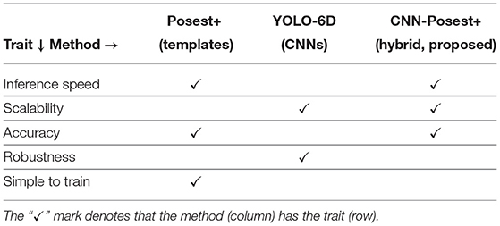
Table 1. The three evaluated methods for 6D object pose estimation from RGB input and their experimentally determined traits.

2. Related Work

Before the explosion of the DNN based techniques, the 6-DoF object pose estimation literature was dominated by feature and template matching methods. More recently, the paradigm shifted to learning based methods and specifically to DNNs. In this section, we focus on methods that use monocular RGB input to perform instance-level 6-DoF object pose estimation. For a deeper analysis and comparison of methods using different input modalities the reader is referred to extensive reviews on the problem (Hodaň et al., 2016; Hodan et al., 2018; Sahin et al., 2020).

Feature/Template Matching Methods: These methods use hand-crafted features and descriptors and template matching. Generally, they operate in two phases: (i) In the training phase, features are extracted from the training images and a database of templates is generated offline, (ii) in the inference phase, features from an input image are extracted and a template matching method is used to identify objects and compute pose. The Posest method of Lourakis and Zabulis (2013) creates a sparse 3D model of each learned object during an offline step using robust local features (Lowe, 1999; Bay et al., 2006; Rublee et al., 2011). These sparse object models are used as a database to retrieve and refine the actual object pose. Payet et al. (Payet and Todorovic, 2011) introduced a Bag of Boundaries representation for their learned objects database, while Tjaden (Tjaden et al., 2017) proposed the use of temporally consistent local color (TCLC) histograms and demonstrated robust results. RAPID-LR (Muñoz et al., 2016) is using a combination of edge matching and HOG descriptors for template matching. Template matching methods do not scale well as the number of objects and their complexity increases. To solve this problem Konishi et al. (2016) proposed the use of hierarchical pose trees (HPT) in their work focusing on pose estimation of texture-less and reflective objects.

Learning Based Methods: These techniques automatically learn the statistics of the objects in a training set. The trained system predicts an intermediate representation that is post-processed to recover the object pose.

Brachmann et al. (2016) proposes a joint classification-regression random forest that predicts object labels and 3D coordinates. In subsequent stages, these predictions are refined using RANSAC and PnP.

CDPN (Li et al., 2019) uses a detector as a first stage to detect the object in the image. On the second stage the proposed Coordinates-based Disentangled Pose Network splits the computation into two paths: The first regresses the object translation, the second regresses 3D coordinates for all object pixels and uses PnP to compute the object rotation. Pix2Pose (Park et al., 2019) also uses a multi stage architecture with a detector in the first stage. Once the object class and 2D bounding box is found, the image crop is fed into a network trained to regress 3D coordinates for each object pixel. The method uses one such network for each class. The full 6D pose is recovered using PnP in a RANSAC scheme.

BB8 (Rad and Lepetit, 2017) uses a CNN based on VGG to segment the object in the image. Subsequently, it feeds the cropped region to another CNN that predicts the 2D coordinates of the object's 3D bounding box corners. The end pose is recovered by applying the PnP algorithm to the 2D-3D correspondences of the corners. PoseCNN (Xiang et al., 2017) also uses a VGG derived DNN to simultaneously detect the center of an object in 2D, its distance from the camera and the rotation of the object in a quaternion representation. The 2D object center is recovered through a Hough voting scheme. While the method can achieve good accuracy, the size of the DNN used and the Hough voting step take a toll on its performance. Oberweger et al. (2018) employs a CNN to generate heatmaps for the location of the 3D bounding box corner projections. The full pose is recovered using a RANSAC scheme on the predicted 2D points. PVNet (Hu et al., 2019; Peng et al., 2019) and DPOD (Zakharov et al., 2019) also take a probabilistic approach. PVNet learns vectors that point to the projections of pre-selected object anchor points. These vectors are generated for each object pixel in the image. The object pose is subsequently recovered using EPnP and the Levenberg-Marquardt algorithm. Hu et al. (2019) segments the object and computes a sparse set of anchor point guesses. Then, the segmentation map is used to filter guesses that belong to the object before applying EPnP to solve for the full object pose. DPOD uses a CNN to compute dense 2D-3D correspondences for each object pixel as well as a segmentation mask. The pose is recovered in post-processing using RANSAC and PnP. CorNet (Pitteri et al., 2019) proposes an oriented corner detector for estimating the pose of industrial objects. A FasterRCNN (Ren et al., 2017) network is used as the corner detector. On the second stage the corners in the image are used along side CAD object models in a RANSAC scheme to identify object classes and object poses. SSD-6D (Kehl et al., 2017) adopts a classification approach for guessing camera viewpoint and in-plane rotation while it is also regressing for 2D bounding box. In the post-processing step, ICP is used to recover the full object pose. Tekin et al. (2018) proposes a more lightweight approach. Using a modified YOLO (Redmon and Farhadi, 2017) detector it regresses to the projected bounding box corners in a single stage architecture. The final pose is recovered using PnP. The method achieves high accuracy and high inference speed.

Assessment of the State-of-the-Art: Template-based methods achieve good accuracy but in most cases require detailed 3D object models to work, they can be sensitive to artifacts and illumination and can have performance issues when dealing with large number of classes. Learning-based methods can be trained end-to-end to perform object detection and 6D pose estimation. In general, learning based methods scale better to multiple objects but are more computationally intensive and require large annotated training datasets and in most cases detailed 3D object models. One can also think of the alternative of designing a hybrid method. More specifically, template matching methods share a common bottleneck on the object detection phase. As the number of templates in the database increases, the performance drops. The number of templates increases with the number and the complexity of the objects. Thus, a hybrid method could combine a learning-based object detection component and a template-based pose estimation one. In this paper we explore this alternative by defining such a method and by evaluating it comparatively to a purely template based and a purely learning-based method.

3. Methods

We present the methods used in our experiments focusing on the reasons they were selected with respect to the requirements described in section 1.

3.1. Posest+

As a representative of the class of template matching methods we consider Posest+, a modified version of the Posest method² proposed by Lourakis and Zabulis (2013). Similar to other template based pose estimation methods, Posest achieves good accuracy and requires very limited computational resources to operate. Posest+ was selected for this comparison for its relaxed learning phase requirements and its capability to achieve good performance on an Intel i7 CPU. Additionally, Posest+ uses local features augmented with depth information for its template representation and does not require a precise CAD model of the target objects.

Posest adopts a Structure from Motion (SfM) technique for acquiring the object models. Instead, Posest+ uses a simpler approach that is compatible to the motivation of this work and which is presented below.

Training: Creating the features and reference poses database is a critical step for the correct operation of the pose estimation pipeline. In order to capture reference RGB images of the objects as well as 3D data for computing the pose, we employed RGB and depth sensors (Smisek et al., 2013).

Training sequence acquisition: For each object we capture an RGB-D video sequence. For optimal results a 360 degree view of the object is needed.

Feature and pose extraction: For each sequence we apply SLAM to extract keyframes and camera poses. There is a number of state of the art methods that can be utilized for this process. For our reference implementation we chose ORBSlam2 (Mur-Artal and Tardós, 2017) and ORB features (Rublee et al., 2011). ORBSlam2 achieves robust camera tracking using features extracted from RGB and depth information. More importantly, the algorithm can fallback to RGB-only features when depth information is missing. This robustness to missing depth is very useful in real world applications, since commonly found reflective or translucent materials make depth acquisition difficult.

Annotation: For each class, a reference camera pose and 3D object boundaries (generated from 2D bounding boxes in reference frames) are supplied by a human annotator. The 3D boundaries are used in order to identify features of background objects.

Detection of the object in each frame of a sequence: For each frame in a training sequence ORBSlam2 provides a camera pose. Using the manually annotated reference pose, all the camera poses are transferred to the reference coordinate system of the object. We extract the ORB features from each frame and use the corresponding depth to compute the 3D point of each feature. Features whose 3D location cannot be computed (i.e., no depth value) are discarded. Finally, we filter the 3D points that lie outside the annotated bounding volume of the object.

Keyframes: We select a number of frames in the sequence where the object is fully visible. Posest uses a Bag of Words (BoW) representation of the ORB features extracted from these “keyframes.” The BoW representations are used to create the object database. The number of keyframes used is a tunable parameter. As a rule of thumb, more keyframes yield better identification and pose estimation results. This also means that larger training sets will yield better results during inference. However, as the experimental results demonstrate, the method performs reasonably well with very few (i.e., less than 10) keyframes.

Inference: The first step in the inference pipeline is to compute the 2D ORB features in the image. From these, a bag of words (BoW) representation is created. We compute the similarity score between the BoW of the query image and all the keyframes in the exhibits database. The set of keyframes that have a similarity score above a threshold constitute the initial “coarse” estimations. The actual pose estimation is achieved with refinement step over this “coarse” estimations. Using the ORB descriptors and matching described in Rublee et al. (2011), we find the best correspondences between the query ORB features of each keyframe. Posest (Lourakis and Zabulis, 2013) is applied to all matches. Posest uses a RANSAC scheme to iteratively select a subset of matches and compute the rigid transformation that best explains the camera motion with respect to a given keyframe pose. The quality of the transformation is measured using the reprojection error of the matched orb features from the query frame to the keyframe. The pose with the best score is selected.

3.2. YOLO-6D

From the broad range of recent 6 DoF pose estimation methods using DNNs, the work by Tekin et al. (2018) was selected for this comparison. This is a single-shot approach for simultaneously detecting an object in an RGB image and predicting its 6D pose. The network proposed by Tekin et al. is based on the popular YOLOv2 (Redmon and Farhadi, 2017) detector. The network learns to predict the location of the 3D bounding box corners of the object as they would appear projected on the image. Subsequently, 6-DoF pose is computed using the PnP algorithm.

In contrast to many probabilistic methods, this method does not require a detailed 3D model of each object for training. This makes the creation and annotation of training sets much simpler. The method achieves state of the art accuracy in common benchmarks. Additionally, the very fast backbone network and the simple post-processing step contribute to a high inference speed (the authors claim 50 fps on a Titan X GPU). In our experiments we used the code provided by the authors³ after adapting it to our multiclass datasets.

We followed the training procedure of Tekin et al. (2018) using SGD with momentum and batch size 8. The same data augmentation parameters were used for jitter, hue, saturation, exposure, crop and scale. No background augmentation was used. The input resolution was set to 416 × 416 pixels which offers the best trade off between accuracy and performance (Tekin et al., 2018). We train the network for a total of 35 epochs using a learning rate of 1e−5 dropping by a factor of 10 after 30 epochs.

3.3. CNN-Posest+ (Proposed)

In order to circumvent the scalability issue, of the template-based methods, we replaced the detection step of the Posest+ pipeline with a Faster-RCNN (Ren et al., 2017) based detector using a Resnet18 (He et al., 2016) backbone. The detector⁴ can perform inference in near realtime even on a mid-range GPU and can be trained to identify hundreds of object classes with high precision and recall at a constant computational cost.

Figure 1 outlines the CNN-Posest+ pipeline. CNN-Posest+ uses the Posest+ for the pose estimation step, thus it still requires the creation of an object database as described in section 3.1. The annotated sequences used for the database generation are also used for training the detector. For this training, we kept the same hyper-parameters as the torchvision implementation, using SGD with momentum and a batch size of 16. Data augmentation with random crop and scale was applied to each training image following the same data augmentation strategy and parameters used in the reference torchvision implementation. We train the detector for a total of 13 epochs using a learning rate of 2e−2 dropping by a factor of 10 after 8 and 11 epochs.

FIGURE 1

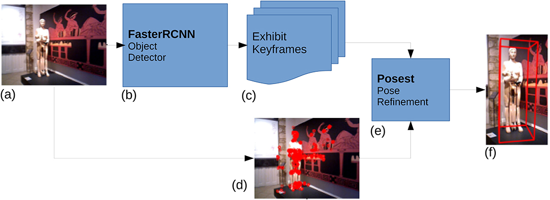
Figure 1. The CNN-Posest+ pipeline: (a) Exhibit input image from the visitor's mobile device, (b) CNN based object detector finds the 2D bbox and id of the exhibit, (c) Exhibit keyframes are selected based on exhibit id, (d) images features are computed, (e) Posest Pose estimation step using (c,d), (f) Exhibit 3D pose is returned to the mobile device.

4. Datasets

We evaluate the three methods on two datasets that are described below.

The YCB92 Dataset: This dataset is derived from the “YCB Video dataset”. YCB Video is a large scale dataset containing 92 video sequences of 21 objects with a total of 133,827 frames. It was created using the objects from the YCB Benchmarks Objects and Models set (Xiang et al., 2017). In each of the 92 video sequences a subset of the 21 objects are placed in a random arrangement on a surface. The surface and background scene change for each sequence. The ground truth provided with the dataset, includes the 6D pose for each object in each frame relative to the camera. Additionally, the models of the objects and the intrinsic parameters of the cameras used are made available.

The default train/validation split of the YCB video dataset has 12 sequences (seq 48-59) reserved for validation and the rest are assigned for training. In the default split the number of objects in the dataset is 21.

We resample the YCB video dataset in order to conform with our real world requirements and the goals of our comparison. Since each sequence in YCB video is shot with a random arrangement of a subset of the objects and on different surfaces and backdrops, we choose to assign each object arrangement (e.g each sequence) as a unique class. This way, the dataset can be thought of as consisting of 92 classes (one for each sequence). We split the frames of each sequence into a training and a validation set.

In order to evaluate the performance change of each method as the number of classes changes, we train and evaluate on four different sub-datasets of YCB92, containing an increasing number of classes: 6, 20, 50, and 92. The selection of sequences for the 6 classes sub-dataset was such that the YCB objects are as diverse as possible (i.e., the sequences do not have many objects in common). This makes the classes differ as much as possible. This special selection is not required for the 20 and 50 classes because the distribution of the objects is more uniform.

For each of the above sub-datasets we created five different train/validation splits in order to evaluate the robustness of the methods with smaller training sets. A common train/validation split in similar datasets (Hinterstoisser et al., 2013) is to use 20% of the total frames for the training set. For YCB92 we use 1, 5, 10, and 20% of the frames for training and the rest for validation. In these splits the training frames are selected uniformly over time from each object sequence. Additionally, we created an extremely restricted training set containing only 3 training frames. In this special case the frames were selected to maximize the coverage of the object. In total, the YCB92 dataset is split into 20 different sub-datasets. The top row of Figure 2, shows three training frames of YCB92.

FIGURE 2

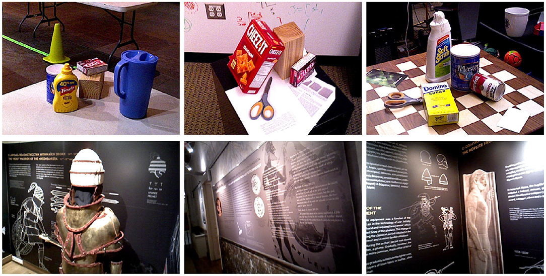
Figure 2. Image samples from the employed datasets. Each image corresponds to a single class. Top: Frames from the YCB92 dataset. All objects and the surface they lay on, are considered as a single object. Bottom: Frames from the Muselearn dataset. Each frame shows a different museum exhibit.

The Muselearn Dataset: The Muselearn dataset consists of two video sequences with a total of 6,212 frames. The dataset is shot in a museum and represents a real world challenge for the methods in our comparison as described in section 1. There is a total of 6 classes in the dataset, each corresponding to a museum exhibit. The dimensions of the exhibits range from 30cm to 2m. The sequences are shot using an RGB-D sensor and the pseudo ground truth is created using a combination of ORBSlam2 (Mur-Artal and Tardós, 2017) and manual exhibit annotation. From the number of frames showing each exhibit we use 20% for training; the rest become the validation set. For the experiments (training and validation) we use only the RGB frames. The bottom row of Figure 2 shows three frames from the Muselearn dataset.

5. Experimental Evaluation

We quantify the effect of (a) increasing the number of object classes and (b) varying the size of the available training set in 6-DoF object pose estimation. We evaluate the translation error E_t and the angular error E_θ (Drost et al., 2010) in 3D space and compare the performance of the three methods. The standard deviation of these errors give a measure of the robustness of each approach. Accuracy A(t) is measured for different thresholds of E_t and E_θ. Specifically, accuracy of A(t) = p means that in p% of the frames the translation error is less than tcm and the rotational error is less than t degrees. Finally, we compute the F1-measure as

$F_1=\frac{2P(t)R(t)}{P(t)+R(t)},$

where P(t) and R(t) are the pose estimation precision and recall for a given accuracy threshold t.

Dataset Balancing: There is a total of 21 datasets used in our comparison, 20 sub-datasets of YCB92 and the Muselearn dataset described in section 4. The number of training frames for a specific class varies from as low as 3 (for the “3 frame” splits) to almost 700 (for some classes in the 20% splits). In order to ensure a fair comparison between all networks for the YOLO-6D and the detector part of the CNN-Posest+ methods, we apply dataset balancing with the following procedure.

In each epoch the network sees 700 images of each object class. This means that for training sets containing less than 700 images of a class, we re-sample from the available images with the class and complement the set up to 700 images through data augmentation. This ensures that during training, all networks see 700 images for each class.

Accuracy as a Function of Number of Classes and Training Set Size: In Figure 3, we compare the accuracy of Posest+, CNN-Posest+, and YOLO-6D as a function of the number of objects/classes and of the training set size. We increase the size of the training set (x-axis: 3 frames, 1, 5, 10, and 20%) and train with sub-datasets containing an increasing number of classes (colored curves: 6, 20, 50, 92). The accuracy A(t) is computed for a threshold t of 2cm and 2°. The results of CNN-Posest+ are virtually identical to the Posest+ results since the two methods share the same pose estimation step. CNN-Posest+ only slightly outperforms Posest+ in some cases where the CNN based detection step is outperforming the template based detection. The most interesting results come from the comparison of Posest+ with YOLO-6D. Posest+ achieves relatively high accuracy even with the most restricted training sets. Additionally, is does not show any degradation in accuracy as the number of classes increases. YOLO-6D achieves competitive accuracy only with larger training sets (≥5%). Additionally, the accuracy of YOLO-6D slightly drops as the number of classes increases.

FIGURE 3

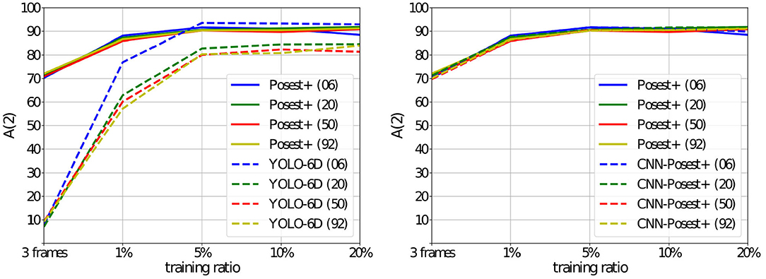
Figure 3. YCB92 Accuracy A(2) for the three methods (the percentage of frames where the 6D pose estimation error is below 2 cm and 2°. The training set size increases on the x-axis. Each curve corresponds to experiments with the same number of classes: 6, 20, 50, and 92. Left: Posest+ vs. YOLO-6D, Right: Posest+ vs. CNN-Posest+.

For a closer examination of the results we focus on the largest training set (20% split). Figure 4 shows the F₁(t) score for different accuracy thresholds t ∈ [1, 10]. YOLO-6D starts to outperform Posest+ for t≥3. Additionally Posest+ is under-performing across the range for the 6 classes sub-datasets. This is explained in detail in the section 5.3).

FIGURE 4

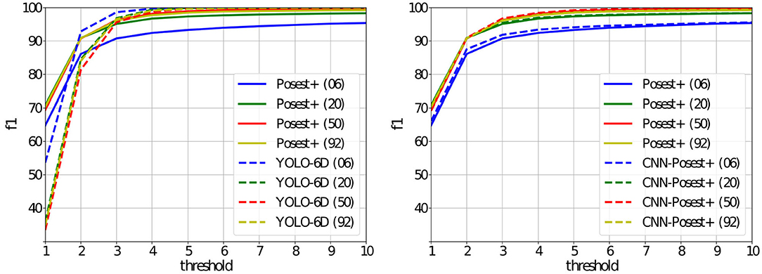
Figure 4. YCB92 f₁(t) score computed for different accuracy thresholds (less than tcm and t°). Only the networks trained with the 20% train/validation split are shown. Left: Posest+ vs. YOLO-6D, Right: Posest+ vs. CNN-Posest+.

The better performance of YOLO-6D for higher thresholds in Figure 4 is explained if we look at the average error and standard deviation (on translation and rotation) for each method. In Figure 5, we examine these metrics for Posest+ and YOLO-6D. For all methods the number of training samples affects the pose estimation error. On the other hand, the increase in the number of classes only affects the learning based method. When training with large enough training sets, the average error both in translation and rotation for the Posest+ method is just slightly lower compared to YOLO-6D. However, Posest+ has a much higher standard deviation producing more noisy results. YOLO-6D is more robust. Interestingly, the deviation of Posest+ drops as the size of the training set increases for all sub-datasets but it is consistently higher than YOLO-6D.

FIGURE 5

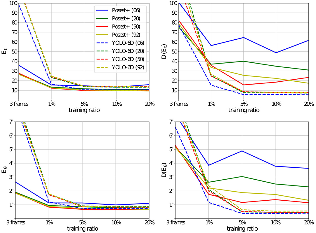
Figure 5. Pose estimation error [E_t and E_θ] and standard deviations [D(E_t) and D(E_θ] for the YCB92 datasets. The training set size increases on the x-axis. Each curve corresponds to experiments with the same number of classes: 6, 20, 50, and 92. Posest+ outperforms the YOLO-6D consistently for the smallest training sets. As the number of training samples increases the difference in the average errors becomes smaller. However, the standard deviation of Posest+ is much higher than that of YOLO-6D.

Method Limitations: We analyze the limitations of the benchmark methods as they emerge from the YCB92 experiments. Figure 6 shows the accuracy A(2) per-class for two 20% split experiments: The 6 and 92 class cases. In the figure we show the classes that are common in both experiments. This way, we compare the effect of learning more classes to the per-class accuracy. On the x-axis we show a representative training image from each of the 6 classes.

FIGURE 6

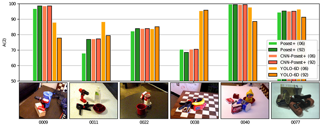
Figure 6. Per-class accuracy A(2) on two YCB92 sub-datasets: For the 20% training ratio we compare the 6 and the 92 class cases. On the x-axis the 6 common objects are shown together with their YCB-Video sequence id.

Template based methods are very sensitive to illumination changes and object texture. While the specifics may vary for different approaches, there are always scenarios that may confuse the template matching pipeline and result to pose estimation failure. Posest+ and CNN-Posest+ use local descriptors to build a bag of words representation of each object. This means that in low texture scenes (i.e., featureless surfaces) or in scenes with repeating patterns the method performs poorly. Moreover, slight changes in the selection of keyframes may result in big differences in the pose estimation accuracy. Learning based methods on the other hand learn features at different scales and thus perform better with repeating textures and can handle better the illumination changes. On the downside, the accuracy of learning based methods decreases as the number of classes increases.

In Figure 6, objects “0038” and “0011” are representative difficult cases for the template based methods. The repeating pattern of the chessboard (“0038”) and the low number of features (“0011”) are the reasons for the low accuracy achieved by Posest+ and CNN-Posest+. This type of cases in YCB92 is the reason for the high standard deviation in translation and angular errors shown in Figure 5. YOLO-6D on the other hand achieves better accuracy in these cases. It is also clear that the per-class accuracy of YOLO-6D drops as the number of classes increases. This drop, however, is not uniform. This could complicate the behavior prediction of a CNN based system as more classes are added. The per-class accuracy of Posest+ and CNN-Posest+ remains constant as more classes are added.

Muselearn Experiments: The Muselearn dataset is closer to our motivational use case with respect to the dataset acquisition procedure as well as the type of classes. It is, however, limited to only 6 museum exhibits. In the bottom row of Figure 2, we show 3 representative frames from the dataset. Figure 7 shows the accuracy A(t) for Posest+ and YOLO-6D. The curves follow the same trend as in the YCB92 datasets. However, Muselearn is more challenging, so the accuracy for both methods is lower. This is also evident in the translation and angular errors shown in Table 2.

FIGURE 7

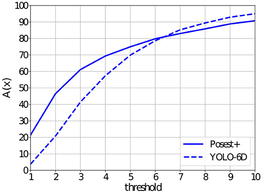
Figure 7. Accuracy A(t) as a function of different thresholds t∈[1, 10] on the Muselearn dataset.

TABLE 2

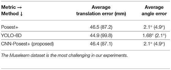
Table 2. Average translation and angular error (and std dev) of the three methods for the Muselearn dataset.

Inference Time: Table 3 shows average inference times in milliseconds per image for each method. All tests were performed on the same mid-range workstation equipped with a 6th generation Intel i7 CPU and an NVIDIA GTX970 GPU. YOLO-6D and CNN-Posest+ feature constant times for different numbers of classes. The inference cost for CNN-Posest+ breaks down to 36ms for the detection step and 92ms for the pose estimation step. For Posest+, inference time is almost linear with the number of classes in the database. It can be approximated by the equation T_inf = 84+0.65N_cl, where N_cl is the number of classes. Note that Posest+ is a CPU only implementation. Even for the 92 classes scenario, YOLO-6D CPU is almost 50% slower than Posest+.

TABLE 3

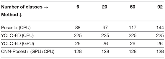
Table 3. Inference times (in ms) for various numbers of classes (sub-datasets of the YCB92).

6. Summary and Conclusions

Driven by the requirements of a real-world application for 6-DoF object pose estimation using a conventional RGB camera, we considered existing approaches that span a broad spectrum of design choices (template-based, learning-based) and we defined a hybrid variant. We evaluated quantitatively these methods based on standard/general and application-tailored datasets that we compiled for this purpose. All three methods conform with the requirements to some degree. According to the summary of the obtained experimental results (see Table 1), the selection of the method to be employed depends on what is considered the most important/critical criterion and other factors, such as the availability of a GPU, whether processing can be offloaded to cloud based services, what are the exact robustness requirements, the maximum number of classes, etc. In a scenario that requires the same, constant accuracy on hundreds of objects with minimum computational cost, Posest+ is the way to go. If robustness is of higher priority and large NNs can be afforded to keep accuracy high, then CNN based methods will deliver at a higher computational cost. For a very large number of exhibits, a good compromise could be the hybrid CNN-Posest+ method. Although this is more complicated to train, computational cost benefits are meaningful in real-world situations involving more than 100 exhibits.

Data Availability Statement

The raw data supporting the conclusions of this article will be made available by the authors, without undue reservation.

Author Contributions

All authors listed have made a substantial, direct and intellectual contribution to the work, and approved it for publication.

Funding

This work was partially supported by the EU and Greek national funds through the Operational Program Competitiveness, Entrepreneurship and Innovation, under the call RESEARCH - CREATE - INNOVATE (project MuseLearn T1EΔK - 00502) and by the H2020-ICT-2016-1-731869 project Co4Robots.

Conflict of Interest

The authors declare that the research was conducted in the absence of any commercial or financial relationships that could be construed as a potential conflict of interest.

Footnotes

1. ^The Muselearn and YCB92 datasets will become publicly available.

2. ^Posest source available in https://users.ics.forth.gr/~lourakis/posest/.

3. ^https://github.com/microsoft/singleshotpose.

4. ^For our implementation, the pytorch-torchvision Faster-RCNN implementation was used https://github.com/pytorch/vision.

References

Bay, H., Tuytelaars, T., and Van Gool, L. (2006). “Surf: speeded up robust features,” in European Conference on Computer Vision (Berlin; Heidelberg: Springer), 404–417. doi: 10.1007/11744023_32

CrossRef Full Text | Google Scholar

Brachmann, E., Michel, F., Krull, A., Ying Yang, M., Gumhold, S., et al. (2016). “Uncertainty-driven 6D pose estimation of objects and scenes from a single RGB image,” in 2016 IEEE Conference on Computer Vision and Pattern Recognition (CVPR) (Las Vegas, NV: IEEE), 3364–3372. doi: 10.1109/CVPR.2016.366

CrossRef Full Text | Google Scholar

Drost, B., Ulrich, M., Navab, N., and Ilic, S. (2010). “Model globally, match locally: efficient and robust 3D object recognition,” in 2010 IEEE Computer Society Conference on Computer Vision and Pattern Recognition (San Francisco, CA: IEEE), 998–1005. doi: 10.1109/CVPR.2010.5540108

CrossRef Full Text | Google Scholar

He, K., Zhang, X., Ren, S., and Sun, J. (2016). “Deep residual learning for image recognition,” in 2016 IEEE Conference on Computer Vision and Pattern Recognition (CVPR) (Las Vegas, NV: IEEE), 770–778. doi: 10.1109/CVPR.2016.90

PubMed Abstract | CrossRef Full Text | Google Scholar

Hinterstoisser, S., Lepetit, V., Ilic, S., Holzer, S., Bradski, G., Konolige, K., et al. (2013). “Model based training, detection and pose estimation of texture-less 3D objects in heavily cluttered scenes,” in Computer Vision - ACCV 2012. Lecture Notes in Computer Science, Vol. 7724, eds K. M. Lee, Y. Matsushita, J. M. Rehg, and Z. Hu (Berlin; Heidelberg: Springer). 548–562. doi: 10.1007/978-3-642-33885-4_60

CrossRef Full Text | Google Scholar

Hodaň, T., Matas, J., and Obdržálek, Š. (2016). “On evaluation of 6D object pose estimation,” in Computer Vision - ECCV 2016 Workshops. ECCV 2016. Lecture Notes in Computer Science, Vol. 9915, eds G. Hua and H. Jégou (Cham: Springer). 606–619. doi: 10.1007/978-3-319-49409-8_52

PubMed Abstract | CrossRef Full Text | Google Scholar

Hodan, T., Michel, F., Brachmann, E., Kehl, W., GlentBuch, A., Kraft, D., et al. (2018). “Bop: benchmark for 6D object pose estimation,” in Computer Vision - ECCV 2018: 15th European Conference, Proceedings, Part III, Vol. 11207, eds V. Ferrari, M. Hebert, C. Sminchisescu, and Y. Weiss (Munich: Springer), 19–34. doi: 10.1007/978-3-030-01249-6_2

PubMed Abstract | CrossRef Full Text | Google Scholar

Hu, Y., Hugonot, J., Fua, P., and Salzmann, M. (2019). “Segmentation-driven 6D object pose estimation,” in 2019 IEEE/CVF Conference on Computer Vision and Pattern Recognition (CVPR) (Long Beach, CA: IEEE), 3380–3389. doi: 10.1109/CVPR.2019.00350

PubMed Abstract | CrossRef Full Text | Google Scholar

Kehl, W., Manhardt, F., Tombari, F., Ilic, S., and Navab, N. (2017). “SSD-6D: Making RGB-based 3D detection and 6D pose estimation great again,” in 2017 IEEE International Conference on Computer Vision (ICCV) (Venice: IEEE), 1530–1538. doi: 10.1109/ICCV.2017.169

CrossRef Full Text | Google Scholar

Konishi, Y., Hanzawa, Y., Kawade, M., and Hashimoto, M. (2016). “Fast 6D pose estimation from a monocular image using hierarchical pose trees,” in Computer Vision - ECCV 2016. ECCV 2016. Lecture Notes in Computer Science, Vol. 9905, eds B. Leibe, J. Matas, N. Sebe, and M. Welling (Cham: Springer). 398–413. doi: 10.1007/978-3-319-46448-0_24

CrossRef Full Text | Google Scholar

Li, Z., Wang, G., and Ji, X. (2019). “CDPN: coordinates-based disentangled pose network for real-time rgb-based 6-dof object pose estimation,” in in 2019 IEEE/CVF International Conference on Computer Vision (ICCV) (Seoul: IEEE), 7678–7687. doi: 10.1109/ICCV.2019.00777

CrossRef Full Text | Google Scholar

Lourakis, M., and Zabulis, X. (2013). “Model-based pose estimation for rigid objects,” in Computer Vision Systems, Volume 7963 of Lecture Notes in Computer Science, eds M. Chen, B. Leibe, and B. Neumann (Berlin; Heidelberg: Springer), 83–92. doi: 10.1007/978-3-642-39402-7_9

CrossRef Full Text | Google Scholar

Lowe, D. G. (1999). “Object recognition from local scale-invariant features,” in Proceedings of the Seventh IEEE International Conference on Computer Vision, Vol. 2 (Kerkyra), 1150–1157. doi: 10.1109/ICCV.1999.790410

CrossRef Full Text | Google Scholar

Muñoz, E., Konishi, Y., Murino, V., and Del Bue, A. (2016). “Fast 6D pose estimation for texture-less objects from a single RGB image,” in 2016 IEEE International Conference on Robotics and Automation (ICRA) (Stockholm: IEEE), 5623–5630. doi: 10.1109/ICRA.2016.7487781

CrossRef Full Text | Google Scholar

Mur-Artal, R., and Tardós, J. D. (2017). ORB-SLAM2: an open-source slam system for monocular, stereo, and RGB-D cameras. IEEE Trans. Robot. 33, 1255–1262. doi: 10.1109/TRO.2017.2705103

CrossRef Full Text | Google Scholar

Oberweger, M., Rad, M., and Lepetit, V. (2018). “Making deep heatmaps robust to partial occlusions for 3D object pose estimation,” in Computer Vision - ECCV 2018. ECCV 2018. Lecture Notes in Computer Science, Vol. 11219, eds V. Ferrari, M. Hebert, C. Sminchisescu, and Y. Weiss (Cham: Springer). 119–134. doi: 10.1007/978-3-030-01267-0_8

CrossRef Full Text | Google Scholar

Park, K., Patten, T., and Vincze, M. (2019). “Pix2pose: pixel-wise coordinate regression of objects for 6D pose estimation,” in 2019 IEEE/CVF International Conference on Computer Vision (ICCV) (Seoul), 7668–7677. doi: 10.1109/ICCV.2019.00776

CrossRef Full Text | Google Scholar

Payet, N., and Todorovic, S. (2011). “From contours to 3D object detection and pose estimation,” in 2011 International Conference on Computer Vision (Barcelona), 983–990. doi: 10.1109/ICCV.2011.6126342

CrossRef Full Text | Google Scholar

Peng, S., Liu, Y., Huang, Q., Zhou, X., and Bao, H. (2019). PVNet: pixel-wise voting network for 6Dof pose estimation,” in 2019 IEEE/CVF Conference on Computer Vision and Pattern Recognition (CVPR) (Long Beach, CA), 4556–4565. doi: 10.1109/CVPR.2019.00469

PubMed Abstract | CrossRef Full Text | Google Scholar

Pitteri, G., Ilic, S., and Lepetit, V. (2019). “CORNet: generic 3D corners for 6D pose estimation of new objects without retraining,” in ICCV Workshops. (Seoul). doi: 10.1109/ICCVW.2019.00342

CrossRef Full Text | Google Scholar

Rad, M., and Lepetit, V. (2017). “BB8: a scalable, accurate, robust to partial occlusion method for predicting the 3D poses of challenging objects without using depth,” in 2017 IEEE International Conference on Computer Vision (ICCV) (Venice), 3848–3856. doi: 10.1109/ICCV.2017.413

CrossRef Full Text | Google Scholar

Redmon, J., and Farhadi, A. (2017). “Yolo9000: better, faster, stronger,” in 2017 IEEE Conference on Computer Vision and Pattern Recognition (CVPR) (Honolulu, HI), 6517–6525. doi: 10.1109/CVPR.2017.690

CrossRef Full Text | Google Scholar

Ren, S., He, K., Girshick, R., and Sun, J. (2017). “Faster r-CNN: towards real-time object detection with region proposal networks,” in IEEE Trans. Pattern Anal. Machine Intell. 39, 1137–1149. doi: 10.1109/TPAMI.2016.2577031

PubMed Abstract | CrossRef Full Text | Google Scholar

Rublee, E., Rabaud, V., Konolige, K., and Bradski, G. (2011). “ORB: an efficient alternative to sift or surf,” in 2011 International Conference on Computer Vision (Barcelona), 2564–2571. doi: 10.1109/ICCV.2011.6126544

CrossRef Full Text | Google Scholar

Sahin, C., Garcia-Hernando, G., Sock, J., and Kim, T.-K. (2020). A review on object pose recovery: from 3D bounding box detectors to full 6D pose estimators. Image Vis. Comput. 96:103898. doi: 10.1016/j.imavis.2020.103898

CrossRef Full Text | Google Scholar

Smisek, J., Jancosek, M., and Pajdla, T. (2013). “3D with kinect,” in Consumer Depth Cameras for Computer Vision. Advances in Computer Vision and Pattern Recognition, eds A. Fossati, J. Gall, H. Grabner, X. Ren, and K. Konolige (London: Springer), 3–25. doi: 10.1007/978-1-4471-4640-7_1

CrossRef Full Text | Google Scholar

Tekin, B., Sinha, S. N., and Fua, P. (2018). Real-time seamless single shot 6D object pose prediction,” in 2018 IEEE/CVF Conference on Computer Vision and Pattern Recognition. (Salt Lake City, UT: IEEE), 292–301. doi: 10.1109/CVPR.2018.00038

CrossRef Full Text | Google Scholar

Tjaden, H., Schwanecke, U., and Schomer, E. (2017). “Real-time monocular pose estimation of 3D objects using temporally consistent local color histograms,” in 2017 IEEE International Conference on Computer Vision (ICCV) (Venice), 124–132. doi: 10.1109/ICCV.2017.23

CrossRef Full Text | Google Scholar

Xiang, Y., Schmidt, T., Narayanan, V., and Fox, D. (2017). PoseCNN: a convolutional neural network for 6D object pose estimation in cluttered scenes. arXiv preprint arXiv:1711.00199. doi: 10.15607/RSS.2018.XIV.019

CrossRef Full Text | Google Scholar

Zakharov, S., Shugurov, I., and Ilic, S. (2019). DPOD: dense 6D pose object detector in RGB images. arXiv preprint arXiv:1902.11020. doi: 10.1109/ICCV.2019.00203

CrossRef Full Text | Google Scholar