Control in Boolean Networks With Model Checking

1. Introduction

The study of control of cellular systems has opened multiple possibilities for application in bioengineering and medicine. It also provides the possibility to make predictions on model behavior, for instance about the reachability of phenotypes under certain mutations, that could be verified experimentally and used for model validation. Experimental approaches for the identification of effective control targets are usually costly and time consuming. To help reducing these efforts, mathematical modeling can be used to identify, in silico, potentially useful interventions that could lead to the reduction of experimental trials [1].

Boolean modeling is often used to model biological systems, since it is able to capture qualitative behaviors by describing the activating or inhibiting interactions between different species using logical functions. The species are represented by binary-valued nodes, whose two activity levels might indicate for instance in a gene-regulatory network whether a certain gene is expressed or not. The simplicity of the Boolean formalism helps coping with the usual problem of lack of parameter information when modeling biological processes while capturing the relevant dynamics of biological systems [2–4].

In the context of control for drug target identification or cell reprogramming, the main goal is the identification of controls that require a minimal number of system interventions. Providing multiple alternatives for minimal control interventions is also desirable, so that suitable interventions for experimental implementation can be found. Furthermore, there are many different scenarios and goals to which control might be applied, for instance, to enforce or avoid a specific behavior in a biological system. An example of such a scenario could be a cell differentiation system where a particular cell type is to be avoided since it can be linked to the development of cancer or another pathology [5].

Many approaches have been developed for control of biological systems, covering different contexts and goals. Some of them focus on leading the system to an attractor of interest, starting from a specific initial state [6] or from any possible initial state [7]. This control problem is known as attractor control. However, in some cases, a small number of observable and measurable components is sufficient to capture the relevant features of the system attractors, for example the set of biomarkers defining a phenotype. In such cases, it might be useful to aim the control toward the phenotype defined by these biomarkers rather than a specific attractor, since fewer interventions might be sufficient. This approach, which targets a set of relevant variables instead of a specific attractor, is known as target control. Several methods have been developed for target control using different computation techniques [8–11].

A basic approach to control is value percolation, which is also a core step in many more sophisticated methods [10, 11]. Approaches based on value percolation can be implemented efficiently [12]. However, they are quite restrictive and might miss many possible control strategies. A step toward the identification of some of these missed control strategies using trap spaces was presented in [9]. Although this approach is more flexible than just value percolation, it also does not identify all the possible control strategies. In the last years, multiple methods have been developed for control strategy identification, looking for instance at the stable motifs of the system [7] or exploiting computational algebra methods [13]. These approaches are usually focused on targeting an attractor or subspace and they also do not generally uncover all possible minimal control strategies. In order to bridge this gap, recent works have tackled the problem of attractor control by using basins of attraction, sets of states from which only a specific attractor is reachable [14]. Such approaches increase in many cases the amount of strategies identified. However, they are still limited to control for attractors and lack flexibility to deal with groups of attractors or phenotypes as well as with attractor avoidance. To the best of our knowledge, there is no method that can identify all the optimal control strategies for a general set of states or attractors.

In this work, we introduce a new approach for control strategy identification that provides a complete solution set of minimal controls and allows full flexibility in the control target. Identifying all the minimal control strategies for a general set of states is a complex problem. It might require the full exploration of the state space, which grows exponentially with the size of the network. To deal with this computational explosion, we explore model checking techniques. Model checking is a verification method that allows one to determine whether a transition system satisfies a specific property. Although originating in the field of computer science, model checking has been successfully applied to analyse biological networks and a wide variety of tools have been developed [15]. Model checking presents many advantages, for instance the use of symbolic representation, which allows one to deal with systems with a large number of states and other problems that could not be handled otherwise. Yet, tackling a wider and more complex control problem naturally entails higher computational costs, since many shortcuts and reduction methods do not apply. Therefore, we investigate efficient preprocessing techniques that can be used to significantly reduce the computational cost and make it suitable for application.

As mentioned above, this work presents a model checking-based method to identify optimal control strategies for any target subset. We start with a general overview about Boolean networks (Section 2). Then we introduce the formal definition of control strategy and show some properties of value percolation that are used in our approach (Section 3). In Section 4, we introduce the main concepts of model checking needed for this work and establish the basis for the control strategy computation with model checking. The implementation of our approach is also detailed in this section, together with techniques to reduce the search space size and improve the performance of the method. Finally, in Section 5 we show the applicability of our method to different biological networks and compare our results with existing control approaches.

2. Background: Boolean Networks and Dynamics

We define a Boolean network as a function f : 𝔹ⁿ → 𝔹ⁿ, with 𝔹 = {0, 1}. The set of variables or components of f is denoted by V = {1, …, n}. Given a Boolean function different dynamics can be defined depending on the way components are updated. A dynamics is usually represented by the state transition graph (STG), a graph whose set of vertices is the state space 𝔹ⁿ and whose edges represent the transitions between them. The synchronous dynamics SD(f) defines transitions that update at the same time all the components that can be updated. Thus, the synchronous state transition graph has an edge from x ∈ 𝔹ⁿ to y ∈ 𝔹ⁿ if and only if x ≠ y and y = f(x). In order to better capture the different times scales that might coexist in a biological system, the asynchronous dynamics AD(f) is often used. It defines transitions that update only one component at a time. Therefore, its state transition graph has an edge from x ∈ 𝔹ⁿ to y ∈ 𝔹ⁿ if there exists i ∈ V such that y_i = f_i(x) ≠ x_i and y_j = x_j for all j ≠ i. The generalized asynchronous dynamics GD(f) includes transitions that update a non-empty subset of components. Thus, given x, y ∈ 𝔹ⁿ there is a transition from x to y if there exists a subset ∅ ≠ I ⊆ V such that y_i = f_i(x) ≠ x_i for all i ∈ I and y_j = x_j for all j ∉ I. To simplify the notation, we use D(f) to refer to any of these three dynamics.

A path in an STG is defined as a sequence of nodes x⁰, x¹, … such that there exists an edge from xⁱ⁻¹ to xⁱ for all i ≥ 1. We denote the set of paths starting in a state x as Paths(x). Given a state x ∈ 𝔹ⁿ, we define Reach(x) = {y ∈ 𝔹ⁿ | ∃π ∈ Paths(x) s.t. y ∈ π} and given S ⊆ 𝔹ⁿ, Reach(S) is the set {y ∈ 𝔹ⁿ | y ∈ Reach(x) for some x ∈ S}. Note that x ∈ Reach(x), since x is the 1-element path to x. A set T ⊆ 𝔹ⁿ such that T = Reach(T) is called a trap set. Trap sets are therefore unions of strongly connected components that do not admit any outgoing edge. An attractor is a minimal trap set under inclusion. Attractors correspond to the terminal strongly connected components of the STG and they might vary in different updates. In biological systems, attractors consisting of only one state (steady states) might correspond to different cell fates, while attractors consisting of more than one state (cyclic attractors) might be associated with sustained oscillation. Figure 1 shows a representation of the three different dynamics (synchronous, asynchronous, and generalized asynchronous) for a Boolean network in four variables. States belonging to attractors are denoted in bold.

FIGURE 1

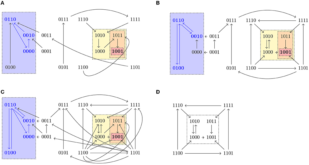
Figure 1. State transition graphs of the Boolean function $f=(x_1{\bar{x}}_2\vee x_1{x}_3\vee x_1{\bar{x}}_4\vee x_2{x}_3{x}_4$, ${\bar{x}}_1{\bar{x}}_2{x}_3\vee {\bar{x}}_1{x}_2{\bar{x}}_3\vee {\bar{x}}_1{x}_3{x}_4$, $x_1{x}_2\vee {\bar{x}}_1{\bar{x}}_2\vee {\bar{x}}_1{x}_2{\bar{x}}_3\vee {\bar{x}}_1{x}_2{x}_4\vee {\bar{x}}_2{\bar{x}}_3{\bar{x}}_4$, ${\bar{x}}_1{x}_2{x}_4\vee x_1{\bar{x}}_2{\bar{x}}_3\vee x_1{x}_2{\bar{x}}_3\vee x_1{\bar{x}}_2{x}_4)$ in (A) synchronous, (B) asynchronous, and (C) general asynchronous dynamics. The trap spaces, denoted by colored boxes, (0∗∗0, 10∗∗, 10∗1, 1001, ∗∗∗∗) and the steady state (1001) are the same in the three dynamics, while the cyclic attractors (marked in blue) vary. All three dynamics admit one cyclic attractor, the set {0110, 0010, 0000} in the synchronous case, {0100, 0110, 0010} in the asynchronous and {0100, 0110, 0010, 0000} in the general asynchronous. (D) Asynchronous dynamics of the restriction of f to Ω = 1∗∗∗, f_↾Ω = (1, 0, $x_2\vee {\bar{x}}_2{\bar{x}}_3{\bar{x}}_4$, ${\bar{x}}_2{\bar{x}}_3\vee x_2{\bar{x}}_3\vee {\bar{x}}_2{x}_4)$. Ω percolates to S = 10∗∗ under f_↾Ω. S is the percolated subspace from Ω with respect to f_↾Ω since S = F(f_↾Ω)(S) and consequently no further percolation is possible.

Given I ⊆ V and c ∈ 𝔹ⁿ we define the subspace induced by I and c as the set Σ(I, c) = {x ∈ 𝔹ⁿ | x_i = c_i ∀i ∈ I}. We denote a subspace by writing the value 0 or 1 for variables that are fixed and ∗ for the free variables. Given a subspace S, we use S_i to denote the value of a fixed component i. For example, 0∗∗1 denotes the subspace fixing the first variable to 0 and the fourth to 1, that is, S = {x ∈ 𝔹ⁿ | x₁ = 0, x₄ = 1} and S₁ = 0 and S₄ = 1. A trap space is a subspace that is also a trap set. Since the minimal subspace containing a state and all of its successors in a state transition graph is the same in all updates, trap spaces of a Boolean network, as opposed to attractors or trap sets, are always the same in any update. The Boolean network shown in Figure 1 has five trap spaces: 0∗∗0, 10∗∗, 10∗1, 1001, ∗∗∗∗.

In this work we consider interventions that fix (or “freeze”) certain components to specific values. Note that a set of such interventions can be seen as a subspace and the effect that these interventions have on the dynamics can be described by restricting the original Boolean function to the intervention subspace. Given a Boolean function f and a subspace Θ = Σ(I, c) we define the restriction of f to the subspace Θ as:

$f_{{\upharpoonright }_{\Theta }}:\Theta \to \Theta ,\text{where for all }i\in V\text{,}(f_{{\upharpoonright }_{\Theta }}{)}_i(x)=\{\begin{array}{ll}{f}_i(x),& i\notin I,\\ c_i,& i\in I.\end{array}$

Note that all the definitions above can be applied to the restriction by identifying f_↾Θ with a Boolean function on 𝔹^n−|I|. An example of the dynamics of a Boolean function restricted to a subspace is shown in Figure 2.

FIGURE 2

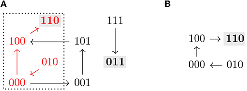
Figure 2. (A) Asynchronous dynamics of the Boolean function $f(x)=({\bar{x}}_2\vee x_1{\bar{x}}_3,x_1{\bar{x}}_3\vee x_2{x}_3,{\bar{x}}_1{\bar{x}}_2\vee x_2{x}_3)$ with two steady states 110 and 011 (marked in gray). The states and paths inside the subspace Ω = ∗∗0 (dotted) are marked in red. (B) Asynchronous dynamics of the restriction of f to Ω = ∗∗0, $f_{{\upharpoonright }_{\Omega }}(x)=({\bar{x}}_2\vee x_1,x_1,0)$. Ω is a control strategy for P = 110 in AD(f). Ω does not percolate to P nor to any non-trivial trap space. T = 110 ⊆ P (in gray) is the only minimal trap space of f_↾Ω and is complete in D(f_↾Ω).

3. Control Strategies: Value Percolation and Completeness

A control strategy is defined as a set of interventions that lead the controlled system to a target subset. This target subset usually represents a specific stable behavior, for instance an attractor or a subspace representing a phenotype. The formal definition of a control strategy is given below.

Definition 3.1. Given a Boolean network f and a subset P ⊆ 𝔹ⁿ, a control strategy for the target P in D(f) is a subspace Θ ⊆ 𝔹ⁿ such that, for any attractor ${A}$ of D(f_↾Θ), ${A}\subseteq P$.

In other words, a subspace Θ = Σ(I, c) is a control strategy for a subset P if fixing the variables in I to their corresponding values in c forces the system to have attractors only in the desired target P. Note that the asynchronous and generalized dynamics for a control strategy can contain non-attractive cycles, which give rise to infinite trajectories that do not reach any attractor. In application, such trajectories are usually viewed as having probability zero and are not further considered in the context of attractor analysis and control. We adopt the same view in this work.

The size of a control strategy Θ = Σ(I, c) is defined as the size of I, and is therefore the number of interventions. Optimal control strategies are the ones with the lowest number of interventions, that is, the maximal subspaces with respect to inclusion. An example of a control strategy is shown in Figure 2, where fixing the variable x₃ = 0 is enough to guarantee that the system only has one attractor, the target steady state 110.

Note that Definition 3.1 considers a subset as the control target, encompassing both attractor control and target control. Moreover, it provides the flexibility to deal with further control problems, such as control to union of attractors ($P={\bigcup }_i{{A}}_i$) or attractor avoidance ($P={𝔹}^n\backslash {A}$).

3.1. Percolation

In this subsection we introduce formally the concept of percolation, used in many approaches to control. We also deduce properties of percolated subspaces that are useful for control strategy identification and that are used later in our approach.

The concept of value percolation is based on the idea that fixing of some components might induce other components to get fixed downstream. We define the percolation function with respect to f as the function that associates to every subspace S the subspace determined by the components fixed by f within S.

Definition 3.2. Given a Boolean function f, the percolation function with respect to f is the function $F(f):{S}\to {S}$, S ↦ F(f)(S), where ${S}$ is the set of all subspaces in 𝔹ⁿ and F(f)(S) is the smallest subspace that contains f(S) (with respect to inclusion).

Explicitly, given a subspace $S\in {S}$, F(f)(S) = Σ(I, c) with I = {i ∈ V | |f_i(S)| = 1} and c any state 𝔹ⁿ such that in c_i = f_i(x) for all x ∈ S for i ∈ I.

Definition 3.3. Let f be a Boolean function and S, S′ ⊆ 𝔹ⁿ two subspaces. We say that the subspace S percolates to S′ under f if and only if there exists k ≥ 0 such that F(f)^k(S) = S′.

For any trap space T and its image T′ = F(f)(T), we have T′ ⊆ T, since by definition F preserves the fixed components of T. The free components in T might get fixed or remain free depending on the Boolean function f. In fact, T′ is a trap space of f, since for any fixed variable i ∈ V in T′, $f_i(x)=T_i^{\prime }$ by definition of F. Moreover, F(f)^k(T) is a trap space for any k ≥ 0. An example of a subspace Ω = 1∗∗∗ percolating to another subspace S = 10∗∗ is shown in Figure 1. Both Ω and S are trap spaces of f_↾Ω.

Remark 3.4. Let f be a Boolean function and S ⊆ 𝔹ⁿ a subspace. Let k ≥ 0 and $S^k=F{(f_{{\upharpoonright }_S})}^k(S)$. Then S^k is a trap space of f_↾S for every k ≥ 0.

Note that the paths in the dynamics of F(f) starting at a trap space T cannot have cycles and, consequently, all the reachable attractors from T in these dynamics are fixed points. When considering the synchronous dynamics of F(f), each initial trap space T leads to a unique fixed point.

Definition 3.5. Given a Boolean function f and a trap space T, we call the unique fixed point T′ of the synchronous dynamics of F(f) reachable from T the percolated subspace from T with respect to f, that is, T′ = F(f)^k(T) with k such that F(f)^k(T) = F(f)^r(T) for all r ≥ k.

In order to relate value percolation to control strategies, we derive some dynamical properties of percolated subspaces.

LEMMA 3.6. Let f be a Boolean function, T ⊆ 𝔹ⁿ a trap space. Let k ≥ 0 and T^k = F(f)^k(T). Then for every x ∈ T there exists a path in D(f) from x to some y ∈ T^k.

PROOF. It is enough to show that if T is a trap space, then for every x ∈ T there exists a path in D(f) from x to some y ∈ F(f)(T). Set T′ = F(f)(T), with I′ ⊆ V being the set of fixed variables in T′. Since T′ ⊆ T, for all i ∈ I′, $f_i(x)=T_i^{\prime }$ by definition of F. Now let us look at every update separately. In the asynchronous dynamics, for every i ∈ I′, x admits a successor y in AD(f) with $y_i=T_i^{\prime }$ and y_j = x_j for j ≠ i; therefore there exists a path from any state in T to T′. In the synchronous dynamics, $f_i(x)=T_i^{\prime }$ for all i ∈ I′ and so x admits a successor y ∈ T′. The case of the generalized asynchronous dynamics follows from the other cases, since all the paths in SD(f) or AD(f) are also paths in GD(f).

COROLLARY 3.6.1. Let f be a Boolean function, S ⊆ 𝔹ⁿ a subspace. Let k ≥ 0 and $S^k=F{(f_{{\upharpoonright }_S})}^k(S)$. Then for every x ∈ S there exists a path in D(f_↾S) from x to some y ∈ S^k.

LEMMA 3.7. Let f be a Boolean function and S ⊆ 𝔹ⁿ a subspace. Let k ≥ 0 and $S^k=F{(f_{{\upharpoonright }_S})}^k(S)$. Then ${A}$ is an attractor of f_↾S if and only if ${A}\subseteq S^k$ and ${A}$ is an attractor of $f_{{\upharpoonright }_{S^k}}$.

PROOF. As noted in Remark 3.4, S^k is a trap space of f_↾S. Then $f_{{\upharpoonright }_S}(x)=f_{{\upharpoonright }_{S^k}}(x)$ for all x ∈ S^k. Therefore, any attractor of $f_{{\upharpoonright }_{S^k}}$ is also an attractor of f_↾S and if ${A}$ is an attractor of f_↾S and ${A}\subseteq S^k$, then ${A}$ is also an attractor of $f_{{\upharpoonright }_{S^k}}$. Let ${A}$ be an attractor of f_↾S. Then ${A}=\text{Reac}{\text{h}}_{f_{{\upharpoonright }_S}}({A})$. By Corollary 3.6.1, for every x ∈ S there exists a path in f_↾S from x to some y ∈ S^k. Therefore, $\text{Reac}{\text{h}}_{f_{{\upharpoonright }_S}}({A})\cap S^k\ne \varnothing$ and so, $S^k\cap {A}\ne \varnothing$. Since S^k is a trap space of f_↾S, ${A}\subseteq S^k$. Therefore, all the attractors of f_↾S are contained in S^k and, consequently, are also attractors of $f_{{\upharpoonright }_{S^k}}$.

COROLLARY 3.7.1. Let f be a Boolean function and S ⊆ 𝔹ⁿ a subspace and P ⊆ 𝔹ⁿ a subset. Let k ≥ 0 and $S^k=F{(f_{{\upharpoonright }_S})}^k(S)$. S is a control strategy for P if and only if S^k is a control strategy for P.

Corollary 3.7.1 provides a way to identify control strategies or discard candidate subspaces by using value percolation. Moreover, checking whether the percolated subspace satisfies the conditions of Definition 3.1 instead of the original subspace allows us to reduce the dimension of the restricted network and, consequently, to simplify the verification problem. In the example shown in Figure 1, it would be enough to check the subspace S to know whether the subspace Ω is a control strategy.

Percolation-only methods select candidate subspaces and percolate them. If the resulting subspace is contained in the target subspace, the candidate subspace is identified as a control strategy [10]. This type of control strategies can be identified efficiently [12]. However, additional control strategies might exist, that do not directly percolate to the target subspace, as shown in [9], or even to non-trivial intermediate trap spaces. An example of this scenario can be seen in Figure 2, where the control strategy Ω does not percolate to the target nor to any non-trivial trap space. With our approach, value percolation can also be exploited as a first step toward control strategy identification, as a means to achieve dimensionality reduction, as described by Corollary 3.7.1.

3.2. Completeness

To improve control detection, we propose to define sufficient conditions on the system restricted to a candidate subspace to identify this candidate as a control strategy. Moreover, conditions on minimal trap spaces can be defined in order to deduce properties of the system attractors, in particular, their belonging to a target subset.

DEFINITION 3.8. A set of trap spaces ${T}$ is complete in D(f) if and only if for every attractor ${A}$ of D(f) there exists $T\in {T}$ such that ${A}\subseteq T$. A Boolean function f is complete in the dynamics D(f) if its minimal trap spaces are complete in D(f).

Completeness of the minimal trap spaces has been used for attractor approximation and it can be detected using model checking as described in [16]. The following proposition presents sufficient conditions for a subspace to be a control strategy. Given a candidate subspace, if the set of minimal trap spaces of the restricted system is complete and contained in the target subset, then the candidate subspace is a control strategy for that subset.

PROPOSITION 3.9. Let f be a Boolean function, P, Θ ⊆ 𝔹ⁿ subspaces and ${T}$ the set of minimal trap spaces of f_↾Θ. If all the trap spaces of ${T}$ are contained in P and ${T}$ is complete in D(f_↾Θ), then Θ is a control strategy of P.

PROOF. Let ${A}$ be an attractor of D(f_↾Θ). Since ${T}$ is complete in D(f_↾Θ), there exists a minimal trap space $T\in {T}$ such that ${A}\subseteq T$. Therefore, ${A}\subseteq T\subseteq P$.

Proposition 3.9 provides sufficient conditions that allow us to identify new control strategies missed by percolation-based approaches. An example of such a control strategy is shown in Figure 2. The subspace Ω is not a trap space nor percolates to any smaller subspace. Since f_↾Ω is complete in AD(f_↾Ω) and its only attractor is included in the target P, Ω is identified as a control strategy. We refer to this approach for control strategy identification as the completeness approach. However, it still does not characterize all the possible control strategies satisfying Definition 3.1. Figure 3 shows a subspace Ω that is a control strategy for the target P but, since Ω is the unique trap space in f_↾Ω and Ω ⊈ P, Proposition 3.9 cannot be applied. Thus, Ω is not detected as a control strategy by the completeness approach. To obtain the full solution set, we formulate a model checking approach, as shown in the next section.

FIGURE 3

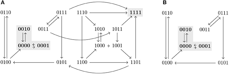
Figure 3. The asynchronous dynamics of a Boolean function f and its restriction f_↾Ω, with Ω = 0∗∗∗, are represented in (A,B), respectively. Attractors are marked in gray. Ω is a control strategy for P = 00∗∗ in AD(f). Ω is not a trap space in f and it does not percolate to the target P nor to any other trap space in f_↾Ω. Since Ω is the unique trap space in f_↾Ω and Ω ⊈ P, Ω would not be identified as control strategy by the completeness approach.

4. Control Strategies With Model Checking

4.1. Model Checking

This section provides a practical introduction to the model checking concepts required for the description of our approach. For a more extensive and detailed explanation of model checking we refer the reader to [17]. Model checking is a formal method used in computer science to solve verification problems. Its application to the control strategy problem presents many advantages, for instance the use of symbolic representation, which allows one to deal with systems with a large number of states, like STGs of Boolean networks. Moreover, many efficient algorithms have been developed and are available for running model checking queries. An overview of existing model checking tools in the context of biochemical networks analysis can be found in [15].

Model checking allows one to verify whether a given transition system satisfies a specific property. A transition system is defined as a set of states and a set of transitions, which represent changes from one state to another. Formally, a labeled transition system (LTS) is defined by a tuple (S,T,L) where S is a finite set of states, T ⊆ S × S is a transition relation such that (x¹, x²) ∈ T if there exists a possible transition from state x¹ to state x² and L : S → 2^AP is a labeling function with AP a finite set of atomic propositions. In the following, a transition (x¹, x²) will also be denoted by x¹ → x². The labeling function L gives a set L(x) ∈ 2^AP of atomic propositions for each state x which includes exactly the atomic propositions satisfied by x. In the Boolean context, an STG defines an LTS, where the set of states is 𝔹ⁿ and the transitions are defined by the Boolean function and the type of update that is chosen. For our purposes, we need a deadlock-free transition system, so we add extra transitions (x, x) ∈ T for every steady state x ∈ 𝔹ⁿ. We use the atomic propositions AP = {(v = c) | v ∈ V, c ∈ 𝔹} and define the labeling function by (v = c) ∈ L(x) if and only if x_v = c.

There are different ways to express properties of a transition system. In our case, we use Computational Tree Logic (CTL). CTL is based on a branching notion of time, where the behavior of the system is represented by a tree of states. In the case of Boolean networks, one can imagine that every path starting in a state x ∈ 𝔹ⁿ is represented as a branch in a tree rooted in x. In the following we introduce the main concepts of CTL.

We distinguish between state properties and path properties. In this context, a path is an infinite sequence x⁰, x¹, … ∈ S such that (xⁱ⁻¹, xⁱ) ∈ T for all i ≥ 1. A statement about a state or a path can be made using a CTL formula. A CTL state formula ϕ over the set of atomic propositions AP is of the form

$\varphi :=a|\neg \varphi |{\varphi }_1\vee {\varphi }_2|{\varphi }_1\wedge {\varphi }_2|\text{E}\phi |\text{A}\phi$

where a ∈ AP is an atomic proposition, E is the exists operator, A is the for all operator, ϕ, ϕ₁, and ϕ₂ are CTL state formulas and φ is a CTL path formula, which in our work will be of the form:

$\phi :=\text{F}\psi |\text{G}\psi$

where F is the future operator, G the global operator, and ψ a CTL state formula. Note that we do not use the full expressiveness of CTL but only a subset of operators necessary to formulate our control queries. In accordance to the definition of semantics of CTL formulas, a state formula is evaluated for a state whereas a path formula is evaluated for an infinite path. When ϕ = a, where a is an atomic proposition, if a ∈ L(x) we say that the CTL state formula ϕ is satisfied at the state x and we write x ⊧ ϕ. For example, if ϕ = (i = 1) for some i ∈ V, then x ⊧ ϕ if (i = 1) ∈ L(x), that is x_i = 1. Analogously, we write π ⊧ φ when the CTL path formula ϕ is satisfied by a path π. See Table 1 for the recursive definition of the satisfaction relation ⊧ for transition systems and CTL formulas used in this work. Since we only use atomic propositions of the form (v = c) where v ∈ V and c ∈ 𝔹 and (v = c) ∈ L(x) if and only if x_v = c, atomic propositions can be interpreted in each state x according to the values of each variable in x. Thus, to simplify the notation, given an atomic proposition ϕ = (v = c), we define ϕ(x) = (x_v = c) so that ϕ is satisfied by x if and only if ϕ(x) = true. Figure 4 shows some examples of state and path formulas which are satisfied in an STG.

TABLE 1

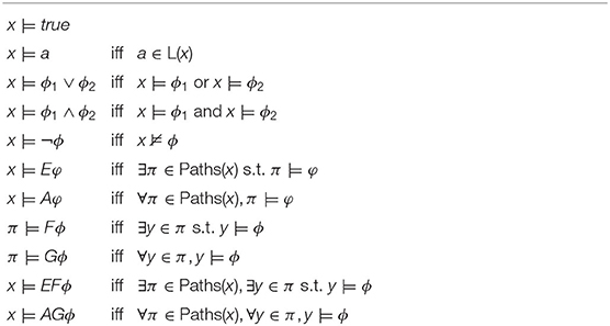
Table 1. Satisfaction relation and semantics for the CTL formulas used in this work, with a ∈ AP an atomic proposition, x ∈ S a state, π a path in the transition system, φ a path formula and ϕ, ϕ₁, and ϕ₂ state formulas.

FIGURE 4

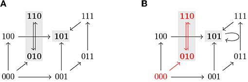
Figure 4. (A) Asynchronous state transition graph of a Boolean function with two attractors, {101} and {010, 110} (marked in gray). (B) TS for the STG shown in (A). Note that a self-loop has been added in the steady state 101 to have a deadlock-free TS. The states 001, 011, 101, and 111 satisfy the state formula AGϕ₃, where ϕ_i = (i = 1), while EFϕ₃ is satisfied by all the states except 010 and 110. The path that starts at 000 and then oscillates between 010 and 110 (in red) satisfies for instance Fϕ₂ and G¬ϕ₃ but not Gϕ₁.

4.2. Control With Model Checking

In this section, we present the basis of our new approach for the identification of all the minimal control strategies, based on model checking. To do so, we express the definition of control strategy in terms of CTL formulas. We start by rewriting it in terms of paths.

LEMMA 4.1. Let f be a Boolean function, Θ ⊆ 𝔹ⁿ a subspace and P ⊆ 𝔹ⁿ a subset. The following are equivalent:

1. Θ is a control strategy for P in D(f).

2. For every x ∈ Θ there exists y ∈ P such that there exists a path in D(f_↾Θ) from x to y and there does not exist any path in D(f_↾Θ) from y to any state outside P (that is, all paths starting at y are contained in P).

PROOF. (⇒) Let x ∈ Θ and let ${A}$ be an attractor of D(f_↾Θ) that can be reached from x. Since Θ is a control strategy, ${A}\subseteq P$. Take $y\in {A}$. Since ${A}$ is reached from x, there exists a path from x to $y\in {A}\subseteq P$ and there are no paths from y leaving P.

(⇐) Let ${A}$ be an attractor of f_↾Θ. Let $x\in {A}$. Since $x\in {A}\subseteq \Theta$, there exists y ∈ P such that there exists a path in D(f_↾Θ) from x to y and there does not exist any path in D(f_↾Θ) from y to any state outside P. Since ${A}$ is an attractor, $y\in {A}$ and $\text{Reac}{\text{h}}_{D(f_{{\upharpoonright }_{\Theta }})}(y)={A}$. Then, ${A}\cap {𝔹}^n\backslash P=\varnothing$, that is, ${A}\subseteq P$, and Θ is a control strategy for P.

Before expressing Lemma 4.1 in terms of CTL formulas, we introduce a state formula ψ_S that is satisfied at a state x if and only if the state x belongs to the subspace S = Σ(I, c):

${\psi }_S(x)={\displaystyle \underset{i\in I}{\wedge }}(x_i=c_i).$

This formulation can be extended to subsets as well. Clearly, every subset can be written as the union of subspaces, since a singleton set constitutes a subspace. Let P ⊆ 𝔹ⁿ be a subset. We define ϕ_P to be satisfied at a state x if and only if the state x belongs to x ∈ P:

${\varphi }_P(x)={\displaystyle \underset{S\in {S}}{\vee }}{\psi }_S(x)$

where ${S}$ is a subspace cover of P.

Now we can express Lemma 4.1 in terms of CTL formulas, using ϕ_P(x) as defined above.

LEMMA 4.2. Let f be a Boolean function, Θ ⊆ 𝔹ⁿ a subspace and P ⊆ 𝔹ⁿ a subset. The following are equivalent:

1. Θ is a control strategy for P in D(f).

2. Φ_P(x), defined as Φ_P(x) = EF(AG(ϕ_P))(x), is satisfied in D(f_↾Θ) for every x ∈ Θ.

PROOF. Φ_P is satisfied at a state x if and only if there exists a path x = x⁰, x¹, … such that AG(ϕ_P) is satisfied at xⁱ for some i ≥ 1. Let y = xⁱ. AG(ϕ_P) is satisfied at y if and only if for all paths y = y⁰, y¹, …, for all i ≥ 0, ϕ_P is satisfied at yⁱ, that is, yⁱ ∈ P. Thus, by Lemma 4.1, Φ_P is satisfied for all x ∈ Θ if and only if Θ is a control strategy for P in D(f).

Note that Φ_P is not affected by the presence of non-attractive cycles since, by definition, they contain at least one state with an outgoing trajectory leading to an attractor.

The CTL formula Φ_P defined in Lemma 4.2 provides a way to determine whether a candidate subspace is a control strategy for P. The next section presents the implementation of this idea for control strategy identification.

4.3. Computation of Control Strategies

Building on the model checking formulas derived in the previous section, we develop a method for control strategy identification. The formula derived in Lemma 4.2 can be used to define a CTL query that can determine whether a candidate subspace is a control strategy for a target subset. In addition, in order to improve the performance of the method, preliminary checks on the candidate subspace and the restricted network can be conducted to possibly discard it without exhaustive exploration. Moreover, the dimension of the problem, that is, the free variables of the Boolean function, can be reduced by restricting the function to the percolated subspace instead of the candidate subspace, as stated in Section 3.1. The complete implementation of the control strategy identification is detailed in Algorithm 1 and explained in the following.

ALGORITHM 1

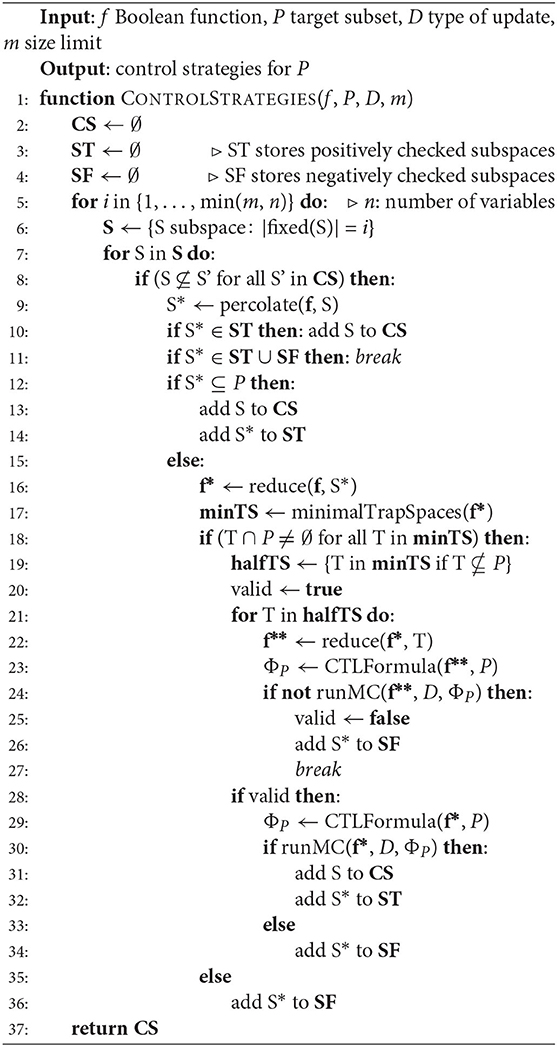
Algorithm 1. Control strategies for a target subset.

The main algorithm takes as inputs a constant-free Boolean function f (i.e. all coordinate functions of f are non-constant), a target subset P and the type of update (asynchronous, synchronous or generalized) and returns the minimal control strategies for P in the respective dynamics. If the original Boolean function is not constant-free, a pre-processing step is applied in which the constant function values are percolated. Instead of the original function we then consider its restriction to the corresponding percolated subspace. As discussed in Section 3.1, this pre-processing does not impact the attractors of the system.

• For each candidate subspace S, its percolated subspace with respect to f_↾S, S^*, is computed (line 9), as defined in Definition 3.5. By Corollary 3.7.1, S^* is a control strategy if and only if S is a control strategy, so we perform all the checks on S^*.

• If S^* is contained in the target subset P, then S is a control strategy (lines 12–13). If not, the algorithm continues to compute the restriction to S^*, f^*, and its minimal trap spaces (lines 16–17).

• If there exists a minimal trap space disjoint from the target, the candidate subspace is discarded, since each minimal trap space contains at least one attractor (line 18).

• Trap spaces that are partially contained in the target subset are analyzed first (line 19). Since f(x) = f_↾T(x) for all x ∈ T, we can reduce the function to T and run the model checking query for the restriction to T, f**, (lines 22–24). If the formula is not satisfied in one of these trap spaces, the candidate subspace is discarded.

• Otherwise, the algorithm concludes by checking the CTL formula Φ_P for the restricted function f^* and deciding whether S is a control strategy (lines 29–30).

Since the aim is to identify optimal control strategies, the candidate subspaces S are taken randomly fixing an increasing number of variables, so that supersets of sets already defining a successful intervention are not considered (lines 5–8). Furthermore, an upper bound m for the size of the control strategies can be set. Moreover, the decisions made for each percolated subspace are stored in two variables ST (for positively checked subspaces) and SF (for negatively checked subspaces) to avoid repeating the same verification query.

The algorithm presented above is implemented using PyBoolNet [18], a Python package that allows generation and analysis of Boolean networks. PyBoolNet uses NuSMV to decide model checking queries for Boolean networks. It also provides an efficient computation of trap spaces for relatively large networks.

5. Results

In this section we study the applicability of our method to different biological networks. We start by applying our method to a network modeling the epithelial-to-mesenchymal transition, considering different control targets: attractor, subspace and subset avoidance. In addition, we compare our approach to current control methods in different Boolean networks for attractor and target control. We show that our method is able to identify all the minimal control strategies identified by other approaches, uncovering in some cases minimal control strategies missed by them. All the results presented here were obtained with a regular desktop 8-processor computer, Intel^®Core^TM i7-2600 CPU at 3.40 GHz, 16 GB memory. The running times vary significantly from scenario to scenario, depending on the type of target considered and the upper bound set on the size of the control strategies. They can range from seconds or minutes, for small control strategies or simple networks, to hours or days of computation for complex target subsets or large control strategies.

5.1. Case Study: EMT Network

The network considered in this case study was recently introduced by Selvaggio et al. [20] to model how microenvironmental signals influence cancer-related phenotypes along the epithelial-to-mesenchymal transition (EMT). The original network consists of 56 components, ten of them being inputs and two readouts or outputs (see Figure 5). Since the original model is multivalued, we work with its booleanized version obtained with GINsim [19]. This booleanization maps a multivalued component of maximum value m to m Boolean components. For instance, a component taking the values 0, 1, 2, 3 is encoded using 3 Boolean variables that would take values 000, 100, 110, 111, respectively (see Table 2). Although this method introduces states that do not correspond to any value of the multivalued variable (non-admissible states), these cannot be part of any attractor since they always have at least one path to an admissible state and do not have incoming transitions from admissible states. Therefore, the asymptotic behavior generated strictly replicates the original model. The booleanized network of this case study consists of 60 Boolean variables, whose regulatory functions can be found in the PyBoolNet repository [18].

FIGURE 5

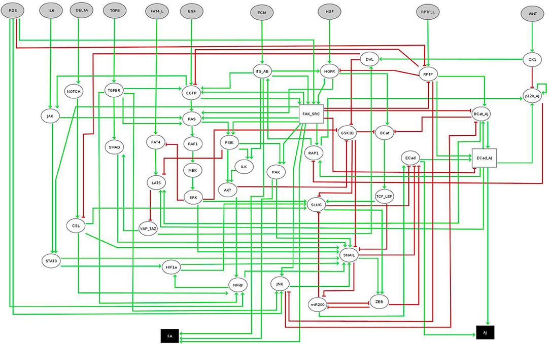
Figure 5. EMT multivalued network. Boolean nodes are represented by ellipses and multivalued nodes by rectangles. Input and output nodes are colored in gray and black respectively. Image obtained using GINsim [19], model from [20]. Further information about the model can be found in [20].

TABLE 2

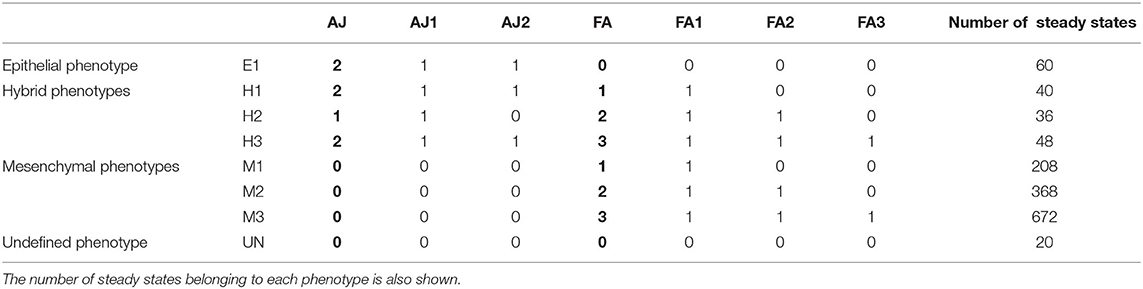
Table 2. Relation of the phenotypes of the EMT network, the values of the multivalued readouts (AJ, FA) in bold, and the values of the equivalent Boolean components (AJ1, AJ2, FA1, FA2, FA3).

The asynchronous dynamics has 1,452 attractors, all of them steady states. They are classified according to the values of the readout components AJ and FA, which represent the different degrees of cell adhesions by adherens junctions and focal adhesions, respectively [20]. The eight resulting biological phenotypes are divided in four groups: epithelial (E1), mesenchymal (M1, M2, M3), hybrid (H1, H2, H3), and unknown (UN) (see Table 2).

To show the flexibility of our method, we analyse different control targets. We start by targeting single steady states (attractor control). Then, we target the subspaces corresponding to each phenotype (target control). Finally, we study the avoidance of the hybrid phenotype, setting as target the complement of the general hybrid phenotype.

5.1.1. Attractor Control: Steady States

Here we consider the problem of attractor control. Since the control targets are steady states, the minimum number of interventions in each control strategy is at least the number of inputs (each input component needs to be fixed to the corresponding value in the attractor).

For each of the 1,452 steady states, the control strategies up to size 13 were identified. Seven hundred and eighty-eight steady states have minimal control strategies of size 10, meaning that the dynamics can be controlled to the steady state only by fixing the values of the input components to their values in the attractor. Of the remaining ones, 396 need an extra component to be fixed, 212 require fixing at least two more components and the last 56 steady states require fixing three extra components.

Figure 6 shows the number of control strategies identified for each size (10–13) with steady states grouped by phenotype, distinguishing between control strategies identified by direct percolation or only by the model checking approach. In most of the cases, our approach is able to identify many control strategies that are missed by direct percolation. In addition, we observe that the mesenchymal phenotypes are the ones with the highest amount of control strategies, which is to be expected since they are also the ones containing more attractors. The number of steady states per phenotype can be found in Table 2. Interestingly, no control strategies consisting of only input variables lead to hybrid steady states.

FIGURE 6

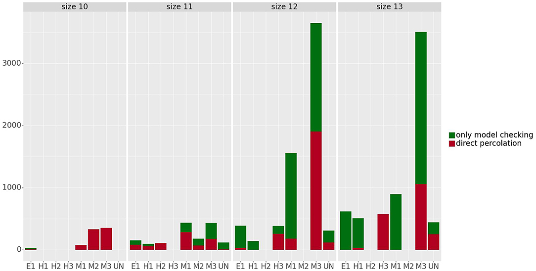
Figure 6. Number of control strategies identified for the steady states grouped by phenotype and size. The control strategies obtained by direct percolation are represented in red and the additional control strategies identified by model checking in green. The number of steady states per phenotype can be found in Table 2.

5.1.2. Target Control

The minimal control strategies up to size 3 are identified for each of the phenotypes, taking as target the subspace defined by the corresponding values of the phenotypic components in each case (see Table 2). The five phenotypic components are excluded from the candidate interventions, since they represent the readouts of the model that we want to control. Table 3 shows the number of control strategies identified per phenotype and size. Similarly to the case of attractor control, we observe that the phenotypes with higher number of control strategies are the mesenchymal phenotypes (over a hundred), while the epithelial and the hybrid phenotypes have fewer or no control strategies up to size 3. This is consistent with the bias of the model toward the mesenchymal phenotypes in terms of attractors.

TABLE 3

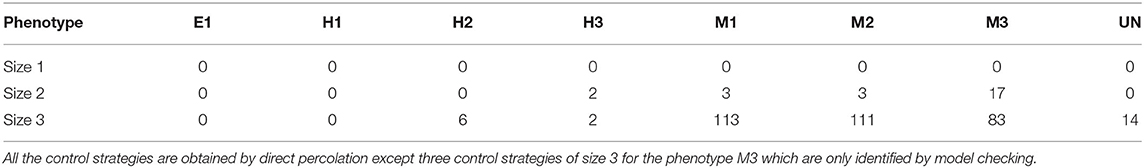
Table 3. Number of minimal control strategies identified per size for each phenotype.

All of the control strategies obtained are also identified by direct percolation, except for three minimal control strategies for the phenotype M3 that are only identified by model checking. These are: {BCat-AJ = 1, GSK3B = 1, ITG-AB = 1}, {ECad-AJ1 = 1, GSK3B = 1, ITG-AB = 1}, and {ECad-AJ2 = 1, GSK3B = 1, ITG-AB = 1}.

5.1.3. Avoidance of Hybrid Phenotypes

According to [20], hybrid phenotypes may provide advantageous abilities to cancer cells such as drug resistance or tumor-initiating potential. Therefore, interventions avoiding these phenotypes might be good candidates for drug targets in therapeutic treatment against cancer cells presenting these traits.

The authors of [20] define the hybrid phenotype as the one containing steady states with both components AJ and FA activated, that is, AJ ≥ 1 and FA ≥ 1. Therefore, the subset defining the avoidance of the hybrid phenotype is

$P=\left\{\text{AJ}1=0,\text{AJ}2=0\right\}\cup \left\{\text{FA}1=0,\text{FA}2=0,\text{FA}3=0\right\}.$

As in the previous case, the five phenotypic components are excluded from the candidate interventions. Setting the upper bound on the size of the control strategies to 1, 12 control strategies are obtained:

$\begin{array}{l}\{\text{ECad}=0\},\{\text{ROS}=1\},\{\text{SLUG}=1\},\{\text{SNAIL}=1\},\{\text{TGFB}=1\},\\ \{\text{TGFBR}=1\},\{\text{ZEB}=1\},\\ \{\text{BCat}=0\},\{\text{CSL}=1\},\{\text{SMAD}=1\},\{\text{TCF-LEF}=0\},\\ \{\text{miR200}=0\}.\end{array}$

The first seven control strategies can be identified using direct percolation to the maximal subspaces of the target subset. The last five are not identified by using only percolation but are captured by the model checking approach. Two of the obtained interventions correspond to input variables (ROS and TGFB) while the other ten correspond to internal components. Looking at the regulatory functions, we observe that TGFBR is uniquely regulated by TGFB, so setting TGFB to 1 implies that TGFBR is also set to 1 and, therefore, these interventions are equivalent in terms of their effect on phenotypic components. Moreover, since there are no control strategies of size 1 for individual phenotypes, we deduce that these interventions lead to systems where multiple phenotypes coexist, none of them being hybrid.

The components involved in the control strategies identified include the epithelial markers (ECad and miR200) and the mesenchymal ones (BCat, SNAIL, SLUG, TCF-LEF, and ZEB) as described in [20]. In addition, the authors of [20] performed a systematic analysis of the effect of single mutants on the attractor landscape, excluding the input variables. All the single mutants corresponding to the non-input interventions found by our approach were identified as having only attractors in non-hybrid phenotypes. Moreover, there was no other single mutation that produced this result. In other words, the results obtained by our approach are in complete correspondence to the ones presented in [20].

5.2. Comparison With Other Methods

In this section, we compare the model checking approach to other control methods currently available. We show that our method is able to capture all the minimal control strategies identified by other methods, uncovering in some cases minimal control strategies that might be missed by them.

In order to be able to compare different approaches, certain common features need to be chosen. Here, we consider control for any possible initial state. We separately compare to methods tackling attractor control and target control. Although approaches for target control can also be used for attractor control when the target attractor is a steady state or minimal trap space, they are usually aimed at targeting larger subspaces, determined for example by a phenotype, which often include several attractors. For this reason, we consider two different scenarios: one for attractor control and one for target control. The case of an arbitrary subset as target could not be considered for comparison, since no other method, to our knowledge, allows this possibility.

The comparison presented here encompasses each of the main approaches for control strategy identification discussed in previous sections (an overview of the main features of the control methods is shown in Table 4):

• For attractor control:

• Stable-motifs approach (SM), attractor control method based on the identification of stable motifs as described in [7].

• Basins approach (BA), attractor control method that uses the basin of attraction of the target attractor to identify control strategies as implemented in [14].

• Model checking approach (MC), as presented in Section 4.

• For target control:

• Percolation-only approach (PO), target control method based on percolation into the target subspace as implemented in [21].

• Trap-spaces approach (TS), target control method based on percolation into selected trap spaces introduced in [9].

• Completeness approach (CN), introduced in Section 3.2.

• Model checking approach (MC), presented in Section 4.

Since the methods for attractor control considered here (BA and SM) only work for asynchronous update, the comparison is only made for this dynamics. In the case of target control, control strategies are identified for both synchronous and asynchronous dynamics.

TABLE 4

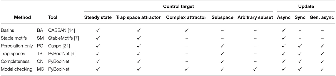
Table 4. Overview of the versatility of the different control methods in terms of the types of targets and update schemes.

In view of the different nature of each method, we do not compare their running times. Some approaches require the computation of the system attractors to identify the control strategies (BA, SM). Others do not allow the choice of a certain attractor as target and identify control strategies for all the attractors simultaneously (SM). Therefore, a fair comparison with respect to the running times is hard to achieve. For this reason, we focus on the amount and size of the control strategies identified, provided that the program terminates within several hours. In particular, our method takes between a few minutes and 2 h for the networks and targets chosen for attractor control and between half an hour and 12 h for the networks and targets chosen for target control.

In order to capture different control scenarios, several biological networks of different sizes with different type and number of attractors are considered. A short description of each network is provided below. See Table 5 for an overview of the networks and their features. The Boolean rules for each biological network can be found in the PyBoolNet repository [18].

1. T-LGL network, introduced by Zhang et al. [4] to model the T cell large granular lymphocyte (T-LGL) survival signaling network. In order for SM to terminate the processing of the network within a few hours, it has been adapted as in [7], removing the outgoing interactions of Apoptosis and setting Stimuli and IL15 to 1 and the remaining inputs to 0. The simplified network consists of 60 Boolean variables and its asynchronous dynamics has 3 cyclic attractors, vs. the 156 (steady states and cyclic) of the original. For sake of simplicity, the same modified network is used for attractor control and target control.

2. MAPK, introduced by Grieco et al. [3] to model the effect of the Mitogen-Activated Protein Kinase (MAPK) pathway on cell fate decisions taken in pathological cells. The network consists of 53 Boolean variables and it has 18 attractors in the asynchronous dynamics, 12 steady states, and 6 cyclic attractors.

3. Cell-Fate network, introduced by Calzone et al. [2] to model the cell fate decision process. The network uses 28 Boolean variables and its asynchronous dynamics has 27 attractors, all of them steady states. These are classified in four different phenotypes (Apoptosis, Survival, Non-Apoptotic Cell Death, and Naive) according to the values of the output components of the network.

As mentioned in Section 4.3, our method takes as input a constant-free Boolean function. Therefore, all the networks with constant coordinate functions considered for comparison have been pre-processed so that the constant values are percolated and removed from the network. In such cases, for the sake of the comparison, all the methods have taken as input the reduced network.

TABLE 5

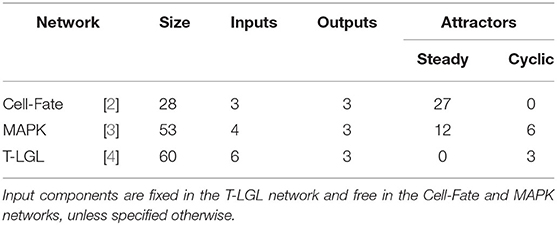
Table 5. Main features of the biological networks used in the comparison.

5.2.1. Attractor Control

We compare our model checking approach (MC) to two methods for attractor control: stable motifs (SM) [7] and basins of attraction (BA) [14]. SM works for steady states and the complex attractors captured by the stable motifs (in some cases, complex attractors are not identified and the method cannot be applied). BA works for any kind of attractors and computes their basins of attraction to identify minimal control strategies.

The control problems selected for each network are described below.

1. T-LGL network. The three attractors of this network can be classified in two types (Survival and Apoptosis) according to the values of the output components. For this comparison, the apoptotic attractor is chosen, that is, the one with Apoptosis = 1. Similar results would be obtained for another choice of attractor.

2. MAPK network. The 18 attractors of this network can also be classified in two types (Survival and Apoptosis) according to the values of the output components. In order to apply BA to this network, we set some input components to fixed values. We consider all the input combinations that allow the two phenotypes to coexist. Three input-value combinations satisfy this condition. For sake of space, we only show the results for one of the combinations, the one fixing EGFR-stimulus = 0 and FGFR3-stimulus = 0 and targeting an apoptotic attractor. Similar results for BA and MC would be obtained for the other input-value combinations and different choices of attractor. Results for SM might vary depending on the target attractor that is chosen.

3. Cell-Fate network. The 27 attractors of this network can be classified in four different phenotypes (Apoptosis, Survival, Non-Apoptotic Cell Death, and Naive) according to the values of the output components. The control strategies up to size 4 obtained by each method for each of the attractors of the network are the same, except for five attractors, where the SM approach missed some of the minimal control strategies obtained by BA and MC. In order to gain more insight, we also compare the results when fixing the input components. We analyse the five input-value combinations that allow the three relevant phenotypes (Apoptosis, Survival, and NonACD) to coexist. For sake of space, we only show the results for one of the combinations, the one fixing FADD = 0, FASL = 1, and TNF = 1 and targeting the apoptotic attractor. Similar results would be obtained for the other input-value combinations and different choices of attractor.

Table 6 contains the size and number of the control strategies up to size 4 computed by each approach for each network. MC is able to identify all the minimal control strategies for every network. SM obtains some non-minimal control strategies of larger size, which are supersets of minimal ones. BA identifies all the minimal control strategies of minimum size, as done by MC. However, while BA does not identify any control strategy larger than the minimum size, MC computes all the strategies minimal with respect to inclusion. The minimal control strategies for each network and the methods that are able to identify them are shown in Table 7.

TABLE 6

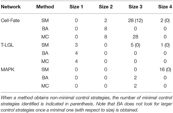
Table 6. Number and size of the control strategies up to size 4 identified by each method (SM, BA, and MC) for the corresponding attractor of each biological network, with the input components fixed as mentioned in the main text.

TABLE 7

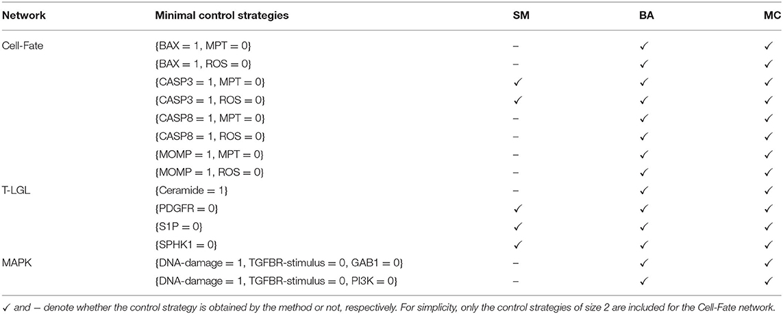
Table 7. Minimal control strategies up to size 4 identified by each method (SM, BA, and MC) for the selected attractor of each biological network.

5.2.2. Target Control

We compare our model checking approach (MC) in asynchronous and synchronous dynamics to several methods for target control: percolation to target (PO) [21], percolation via trap spaces (TS) [9], and the completeness approach (CN), developed in Section 3.2. An overview of the features of each control method is shown in Table 4.

The target subspaces chosen for each network are the ones corresponding to the apoptotic phenotype, a common target in drug identification studies for cancer therapeutic treatments [22]. They are defined in terms of the output components of each network:

1. T-LGL: {Apoptosis = 1, Proliferation = 0}.

2. MAPK: {Apoptosis = 1, Proliferation = 0, Growth-Arrest = 1}.

3. Cell-Fate: {Apoptosis = 1, Survival = 0, NonACD = 0}.

Table 8 contains the size and number of the control strategies computed by each approach for the asynchronous and synchronous dynamics. It is important to note that all the minimal control strategies obtained by PO are included in the ones identified by TS, since TS is built on top of PO. Moreover, direct percolation is a pre-check for CN and MC methods and, therefore, all minimal control strategies found by PO are obtained by CN and MS as well. PO is able to identify a high number of minimal control strategies, as is to be expected since regulatory functions modeling biological systems usually induce a lot of percolation. Nonetheless, in some networks this number is still far from the number of minimal control strategies identified by MC.

TABLE 8

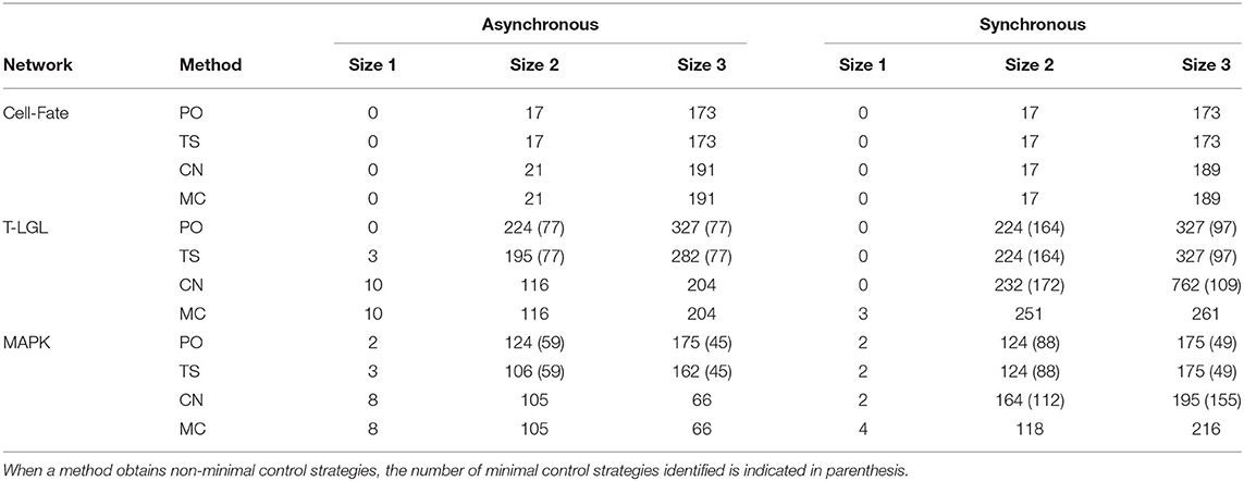
Table 8. Number and size of the control strategies identified by each method (PO, TS, CN, and MC) for the corresponding target subspace of each biological network in the asynchronous and synchronous dynamics.

Control strategies are update-dependent by definition. However, all the control strategies identified by PO are valid in all the dynamics considered here. The number of these control strategies that are minimal might vary from one update to another (see results for T-LGL and MAPK networks). On the other hand, methods TS, CN, and MC are sensitive to the update. In the case of TS, since none of the networks is complete in the synchronous dynamics, attractors cannot be approximated by minimal trap spaces and, therefore, no additional control strategies compared to PO are obtained. Interestingly, the methods CN and MC obtain the same number of control strategies for the asynchronous dynamics. This is not the case for the synchronous dynamics, where additional control strategies are obtained by MC for the T-LGL and MAPK networks. This is caused by the fact that the CN method cannot classify a subspace as a control strategy if the restricted network is not complete. The CN method is likely to obtain better results when the original network is complete, which is usually the case for the asynchronous dynamics of biological networks [16].

These case studies illustrate how an exhaustive approach like the one provided by the model checking method introduced in this article has the capacity to identify, in networks of practical relevance, simple sets of interventions that might otherwise not be identified, and that can furnish additional insights into the model, widening the possibility for potential applications.

6. Discussion

This work presents a novel method to identify all the minimal control strategies for an arbitrary target subset. It is able to deal not only with the problems of attractor control and target control, already tackled by existing methods, but also with subset control, providing maximal flexibility on the definition of the control goal and allowing for instance the possibility of dealing with attractor avoidance problems.

The comparison performed in Section 5.2 shows that our approach is able to identify all the minimal control strategies obtained by the methods analyzed and, in many cases, to uncover new control strategies. It also provides flexibility to study different control problems, which can lead to additional insights into the network. For these reasons, the method presented here can be a good option when a deep analysis of the control strategies of the model is required.

Even though running times are not compared in this work, the model checking approach is likely to entail more computational time than other approaches due to its exhaustiveness, since in some cases the full exploration of the state space might be required. Although the use of symbolic states allows one to deal with relatively large networks, the computational time required to explore their state spaces might still be too high. For this reason, several steps have been developed to reduce the candidate space and the dimensionality of the problem, improving the overall performance. The case studies of Section 5 show the applicability of the method to real models of interest. In cases where this reduction might still be insufficient, our approach could be used to complement faster methods for the particular scenarios in which a more exhaustive analysis is needed.

This new approach is able to adapt to different types of targets and updates. This flexibility, provided by the versatility of model checking, results in the potential to be extended to other control problems. Possible future works could include its extension to tackle control from a set of initial states or the addition of other types of interventions.

Data Availability Statement

Publicly available datasets were analyzed in this study. This data can be found at: https://github.com/hklarner/pyboolnet/tree/master/pyboolnet/repository. The implementation of the method presented in this work can be found in PyBoolNet, in the module control_strategies.py.

Author Contributions

LC-F, ET, and HS conceived the study. LC-F developed the underlying theory, the code, and the analysis with the support of ET. LC-F wrote the manuscript, with contributions from ET and HS. All authors approved the final manuscript.

Funding

LC-F was partially funded by the Volkswagen Stiftung (Volkswagen Foundation) under the funding initiative Life?—A fresh scientific approach to the basic principles of life (Project ID: 93063).

Conflict of Interest

The authors declare that the research was conducted in the absence of any commercial or financial relationships that could be construed as a potential conflict of interest.

Publisher's Note

All claims expressed in this article are solely those of the authors and do not necessarily represent those of their affiliated organizations, or those of the publisher, the editors and the reviewers. Any product that may be evaluated in this article, or claim that may be made by its manufacturer, is not guaranteed or endorsed by the publisher.

Acknowledgments

We would like to thank Claudine Chaouiya, Florence Janody, and Hannes Klarner for fruitful discussions. We acknowledge support by the Open Access Publication Initiative of Freie Universität Berlin.

References

1. Flobak Å, Baudot A, Remy E, Thommesen L, Thieffry D, Kuiper M, et al. Discovery of drug synergies in gastric cancer cells predicted by logical modeling. PLoS Comput Biol. (2015) 11:e1004426. doi: 10.1371/journal.pcbi.1004426

PubMed Abstract | CrossRef Full Text | Google Scholar

2. Calzone L, Tournier L, Fourquet S, Thieffry D, Zhivotovsky B, Barillot E, et al. Mathematical modelling of cell-fate decision in response to death receptor engagement. PLoS Comput Biol. (2010) 6:e1000702. doi: 10.1371/journal.pcbi.1000702

PubMed Abstract | CrossRef Full Text | Google Scholar

3. Grieco L, Calzone L, Bernard-Pierrot I, Radvanyi F, Kahn-Perlès B, Thieffry D. Integrative modelling of the influence of MAPK network on cancer cell fate decision. PLoS Comput Biol. (2013) 9:e1003286. doi: 10.1371/journal.pcbi.1003286

PubMed Abstract | CrossRef Full Text | Google Scholar

4. Zhang R, Shah MV, Yang J, Nyland SB, Liu X, Yun JK, et al. Network model of survival signaling in large granular lymphocyte leukemia. Proc Natl Acad Sci USA. (2008) 105:16308–13. doi: 10.1073/pnas.0806447105

PubMed Abstract | CrossRef Full Text | Google Scholar

5. Dongre A, Weinberg RA. New insights into the mechanisms of epithelial-mesenchymal transition and implications for cancer. Nat Rev Mol Cell Biol. (2019) 20:69–84. doi: 10.1038/s41580-018-0080-4

PubMed Abstract | CrossRef Full Text | Google Scholar

6. Mandon H, Su C, Haar S, Pang J, Paulevé L. Sequential reprogramming of Boolean networks made practical. In: Bortolussi L, Sanguinetti G, editors. Computational Methods in Systems Biology. Vol. 11773. Cham: Springer International Publishing (2019). p. 3–19. doi: 10.1007/978-3-030-31304-3_1

CrossRef Full Text | Google Scholar

7. Zañudo JGT, Albert R. Cell fate reprogramming by control of intracellular network dynamics. PLoS Comput Biol. (2015) 11:e1004193. doi: 10.1371/journal.pcbi.1004193

PubMed Abstract | CrossRef Full Text | Google Scholar

8. Biane C, Delaplace F. Causal reasoning on boolean control networks based on abduction: theory and application to cancer drug discovery. IEEE/ACM Trans Comput Biol Bioinform. (2019) 16:1574–85. doi: 10.1109/TCBB.2018.2889102

PubMed Abstract | CrossRef Full Text | Google Scholar

9. Cifuentes Fontanals L, Tonello E, Siebert H. Control strategy identification via trap spaces in Boolean networks. In: Abate A, Petrov T, Wolf V, editors. Computational Methods in Systems Biology. Cham: Springer International Publishing (2020). p. 159–75. doi: 10.1007/978-3-030-60327-4_9

CrossRef Full Text | Google Scholar

10. Samaga R, Kamp AV, Klamt S. Computing combinatorial intervention strategies and failure modes in signaling networks. J Comput Biol. (2010) 17:39–53. doi: 10.1089/cmb.2009.0121

PubMed Abstract | CrossRef Full Text | Google Scholar

11. Yang G, Gómez Tejeda Zañudo J, Albert R. Target control in logical models using the domain of influence of nodes. Front Physiol. (2018) 9:454. doi: 10.3389/fphys.2018.00454

PubMed Abstract | CrossRef Full Text | Google Scholar

12. Kaminski R, Schaub T, Siegel A, Videla S. Minimal intervention strategies in logical signaling networks with ASP. Theory Pract Logic Programm. (2013) 13:675–90. doi: 10.1017/S1471068413000422

CrossRef Full Text | Google Scholar

13. Murrugarra D, Veliz-Cuba A, Aguilar B, Laubenbacher R. Identification of control targets in Boolean molecular network models via computational algebra. BMC Syst Biol. (2016) 10:94. doi: 10.1186/s12918-016-0332-x

PubMed Abstract | CrossRef Full Text | Google Scholar

14. Su C, Pang J. CABEAN: a software for the control of asynchronous Boolean networks. Bioinformatics. (2020) 37:879–81. doi: 10.1093/bioinformatics/btaa752

PubMed Abstract | CrossRef Full Text | Google Scholar

15. Carrillo M, Góngora PA, Rosenblueth D. An overview of existing modeling tools making use of model checking in the analysis of biochemical networks. Front Plant Sci. (2012) 3:155. doi: 10.3389/fpls.2012.00155

PubMed Abstract | CrossRef Full Text | Google Scholar

16. Klarner H, Siebert H. Approximating attractors of Boolean networks by iterative CTL model checking. Front Bioeng Biotechnol. (2015) 3:130. doi: 10.3389/fbioe.2015.00130

PubMed Abstract | CrossRef Full Text | Google Scholar

17. Baier C, Katoen JP. Principles of Model Checking. Cambridge, MA; London: MIT Press (2008).

Google Scholar

18. Klarner H, Streck A, Siebert H. PyBoolNet: a Python package for the generation, analysis and visualization of Boolean networks. Bioinformatics. (2016) 33:770–2. doi: 10.1093/bioinformatics/btw682

PubMed Abstract | CrossRef Full Text | Google Scholar

19. Chaouiya C, Naldi A, Thieffry D. Logical modelling of gene regulatory networks with GINsim. Methods Mol Biol. (2012). 804:463–79. doi: 10.1007/978-1-61779-361-5_23

PubMed Abstract | CrossRef Full Text | Google Scholar

20. Selvaggio G, Canato S, Pawar A, Monteiro PT, Guerreiro PS, Brás MM, et al. Hybrid epithelial-mesenchymal phenotypes are controlled by microenvironmental factors. Cancer Res. (2020) 80:2407–20. doi: 10.1158/0008-5472.CAN-19-3147

PubMed Abstract | CrossRef Full Text | Google Scholar

21. Videla S, Saez-Rodriguez J, Guziolowski C, Siegel A. Caspo: a toolbox for automated reasoning on the response of logical signaling networks families. Bioinformatics. (2016) 33:947–50. doi: 10.1093/bioinformatics/btw738

PubMed Abstract | CrossRef Full Text | Google Scholar

22. Carneiro BA, El-Deiry WS. Targeting apoptosis in cancer therapy. Nat Rev Clin Oncol. (2020) 17:395–417. doi: 10.1038/s41571-020-0341-y

PubMed Abstract | CrossRef Full Text | Google Scholar