Face Recognition in Single Sample Per Person Fusing Multi-Scale Features Extraction and Virtual Sample Generation Methods

1. Introduction

Face recognition is a biometric recognition technology, which is one of the most active research fields in computer vision and pattern recognition in recent years. It can be used in identity recognition [1], access control, forensics, human-computer interaction, and other fields [2, 3].

At present, there are many methods for face recognition, but there are still many problems to be solved, such as Single Sample Per Person (SSPP) face recognition. In most practical cases, there is only one example per individual to train the system for SSPP, which makes it difficult to identify individuals in an unconstrained environment, mainly when dealing with changes in facial expressions, posture, lighting, and occlusion [4]. In addition, the more difficult challenge is the scenario where these problems coexist, which requires a robust way to handle potentially corrupted SSPP images. In recent years, a great deal of research has been carried out in this field, with some promising but not satisfactory results [5, 6].

There are several methods to solve the problem of SSPP face recognition: virtual sample generation, patch-based method, an image segmentation method, generic learning method, and so on [7–10]. Among these methods, virtual sample generation is a commonly used method to generate more samples. In general, virtual samples are generated from the original single sample, resulting in too much similarity between the samples. This does not guarantee the recognition performance of SSPP, especially under the influence of illumination and expression. In order to improve the recognition performance of SSPP, some novel and improved methods have been studied in recent years. For example, Choi et al. proposed an effective coupled bilinear model, which uses a single image to generate virtual images under different lighting conditions [11]. Hong et al. proposed a virtual sample generation method, which uses a 3D face model to generate synthetic images of different poses to create visual samples [12]. Moreover, Tingwei et al. proposed a new face recognition method that uses a decision pyramid classifier with large appearance variation to divide each training image into multiple non-overlapping local blocks [5].

Feature extraction is also widely used to solve SSPP face recognition problem. For example, Fan et al. proposed a binary coding feature extraction method for single sample face recognition, which combines a self-organizing map network and a bag-of-feature model to extract middle-level semantic features, and used a descriptor to extract local features of facial images [13]. Yang et al. proposed a feature extraction method based on a fully robust local region, which utilizes a convolutional neural network to carry out adaptive convolution of the local region and to discriminate the face identity [14]. Moreover, Xing et al. extracted robust triple local features such as Gabor facial features with multiple scales and directions from different facial local regions [9]. In addition, Adjabi et al. discussed the implementation of multi-block color binarization statistical image features for SSPP face recognition by using the correlation of local, regional, global, and texture-color features [15].

Although the above methods improve the performance of face recognition to a certain extent, the problem of poor robustness cannot be solved completely due to the lack of various face samples [10].

The highlights of this article include the following:

A virtual sample generation method, namely Non-negative Matrix Factorization (NMF) reconstruction strategy with Mirror transform(M), Sliding window(S) and Bit plane(B) sample extension methods, is proposed based on the single sample;

A WPD-HOG-P feature extraction method is proposed on the fusion of Wavelet Packet Decomposition (WPD), Histogram of Oriented Gradient (HOG), and image pyramid strategy;

Support Vector Machine (SVM) algorithm is employed to construct the facial recognition model;

Experiments over ORL and FERET sets are conducted to verify the efficiency of the proposed methods.

The rest of the article is organized as follows. Section 2 gives a brief introduction to the related work. Section 3 presents the theoretical basis of virtual sample generation and feature extraction methods, and Section 4 introduces the proposed virtual sample generation method. Next, the WPD-HOG feature extraction method is introduced in Section 5. Section 6 introduces the experiments and analysis of experimental results. Finally, Section 7 concludes the article.

2. Related Work

This section reviews related work from two aspects of virtual sample generation and feature extraction. On this basis, the technical gaps of SSPP face recognition are determined, so as to promote our research on SSPP face recognition.

2.1. Virtual Sample Generation Method

From the review of literature, many well-known solutions to the SSPP problem have been proposed, although a full review of this area is beyond the scope of this article. Popular virtual sample generation methods in SSPP face recognition mainly include the sample expansion method [16, 17], image enhancement method [12, 18], feature subspace expansion method [19–22], general learning framework method [23–25], 3D identification method [26, 27], and so on. This article focuses on the method of sample expansion. On this basis, a new feature extraction method is proposed.

Sample expansion is one of the most typical methods to solve SSPP problems including geometric distortion, photometric transformation, and perturbation methods, and so on. The purpose is to generate a rich set of training samples and improve the recognition performance of SSPP. For example, Zhang et al. proposed a method to combine the original training sample and its virtual mirror symmetry plane into a new training sample set [16]. For another example, Jinsu et al. proposed a general sliding window method, which uses the large window and small length mechanism to collect and expand window images [17]. This method not only increases the training sample but also fully preserves and strengthens the intra-class and inter-class information inherent in the original sample pattern. In addition, Min et al. proposed a sample expansion method of feature space, namely K-class feature transfer, in order to enrich the in-class variation information of single sample face features [21]. Experimental results showed the effectiveness and robustness of the proposed method.

Non-negative Matrix Factorization is a method to constrain all values in a matrix to be non-negative, making it easier to check. This method can be used for high-quality virtual sample reconstruction. The application of NMF in face recognition is generally to expand face image samples. These virtual samples can more effectively represent the internal relationship between different parts of the face and express the face information. For example, Wen-Sheng et al. studied NMF and proposed a kernel non-negative matrix decomposition algorithm based on block segmentation [23]. Furthermore, Yuwu et al. presented a series of improvements to NMF [24]. Experimental results showed that the proposed algorithm is robust and effective in image classification and feature extraction. Virtual Sample Generation Methods in SSPP face recognition are expressed in Table 1.

TABLE 1

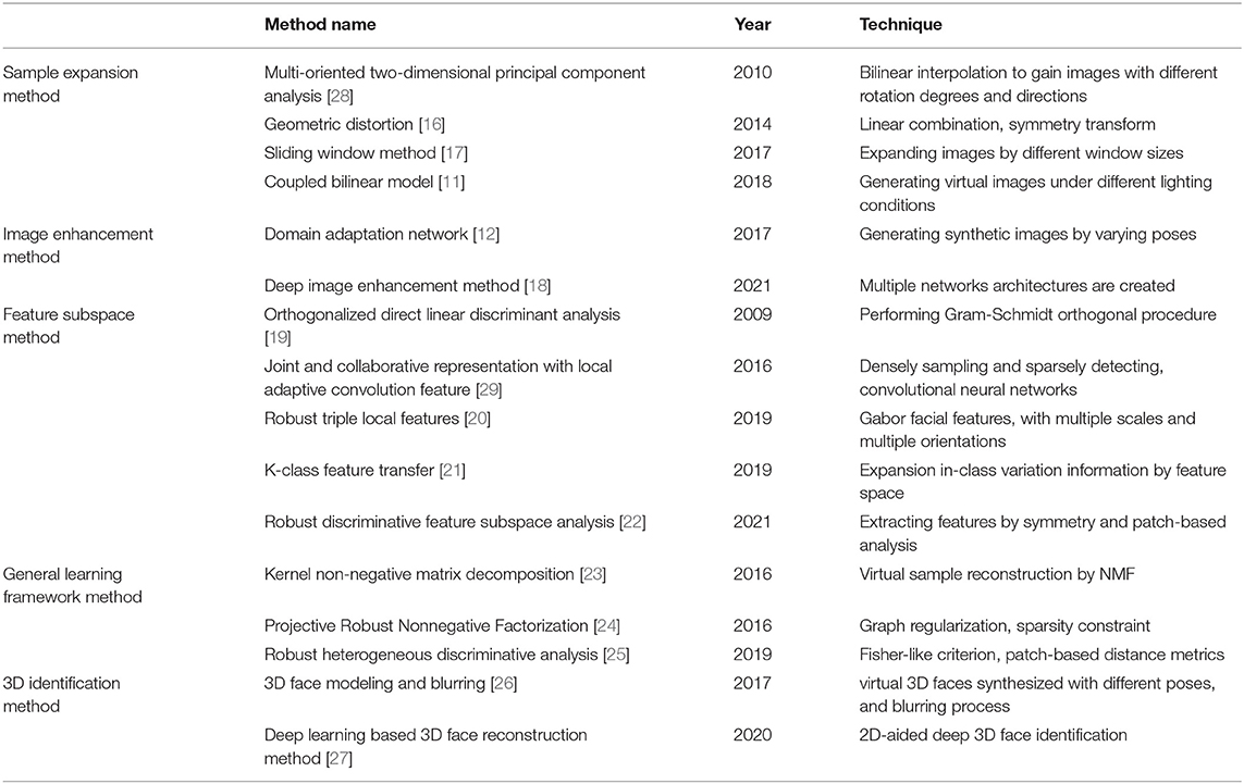
Table 1. Comparison of different virtual sample generation methods in Single Sample Per Person (SSPP) face recognition.

2.2. Feature Extraction Method

The commonly used feature extraction methods can be roughly divided into the following categories: global feature extraction method, local feature extraction method, and the combination of the two methods [30]. By linking the grayscale values of all the pixels of the face image, the global feature can be regarded as a high-dimensional vector. Local features can be regarded as short vectors that describe specific areas in the face image, such as eyes, nose, mouth, etc.

The advantage of the global feature method is that it can retain more useful details of face recognition than that based on local features. At the same time, there are some disadvantages. The contradiction between high-dimensional image data and small samples is more serious. Since each class has only one vector, the in-class variation can no longer be estimated directly [31]. Typical global feature methods include Principal Component Analysis (PCA) [32, 33], Linear Discriminant Analysis (LDA) [34], and so on.

Compared with the global feature method, the local feature extraction method may be more suitable for the SSPP face recognition problem. The reasons are as follows: first, the original face is represented by a set of low-dimensional local features, rather than a single full-high-dimensional vector, thus avoiding the dimension curse problem. Second, the local method can easily identify common and class-specific features, which provide additional flexibility for face recognition based on partial face images. Local features can provide different facial features, increasing the diversity of classifiers. This is beneficial to improve the performance of the SSPP face recognition problem. Therefore, many methods based on local features have been proposed in recent years, such as Local Binary Pattern (LBP) [35], Gabor transform [36], Histogram of Oriented Gradient (HOG) [37], etc.

Both global and local feature extraction methods have their own characteristics and advantages. Global feature representation is robust and helps to identify areas such as forehead and cheek, while local feature representation can represent facial changes. Combined, the two can give full play to their respective strengths. PCA is a typical global feature extraction method, which can extract the global gray feature of the whole image. LBP can extract local gray-scale features, such as mouth area features. For example, Karanwal et al. introduced a hybrid method of PCA and LBP [38]. However, the extensibility of this method is vulnerable. Moreover, Sharifnejad proposed an expression recognition algorithm based on a pyramid histogram for gradient feature extraction [39]. The pyramid based face image can be constructed by multi-scale analysis, which can effectively extract the global and local features of the face. However, it has the problem of high dimensions and high computational complexity. In addition, Guo et al. proposed a new two-layer local-to-global feature learning framework, which leverages local information as well as global information [40]. However, this method also has the problem of high computational complexity.

In recent years, convolutional neural networks (CNN) have become a powerful tool to solve many problems existing in machine learning and biometrics. This development was inspired by the biology of human vision [41]. Some new models based on CNN have been developed for solving the SSPP problem. For example, Junying et al. provided an in-class variation set to expand a single sample, which introduces a well-trained deep convolutional neural networks (DCNN) model by using transfer learning [42]. The experimental results showed that the combination of the traditional method with deep learning achieves good performance in SSPP face recognition. Moreover, Bodini et al. proposed a feature extraction method based on DCNN, which combines the effectiveness of DCNN with the excellent capability of LDA for SSPP [43]. Furthermore, Sungeun et al. proposed an SSPP domain adaptive network architecture based on the combination of depth architecture and domain confrontation training [12]. Lastly, Tewari et al. proposed a new model-based deep convolution autoencoder that solves the challenging problem of reconstructing 3D faces from a single wild color image. Its core innovation is a differential parameter decoder based on the generation model to analyze and encapsulate the image formation [44].

Although CNN has shown good performance in SSPP face recognition, there are still some problems in the training of CNN-based architecture, such as overfitting, hyperparameter, high computational complexity, and large amount of data [2]. Especially for the SSPP problem, the traditional virtual sample expansion methods are still used to generate effective samples [12, 42]. Table 2 gives the comparison of existing feature extraction methods.

TABLE 2

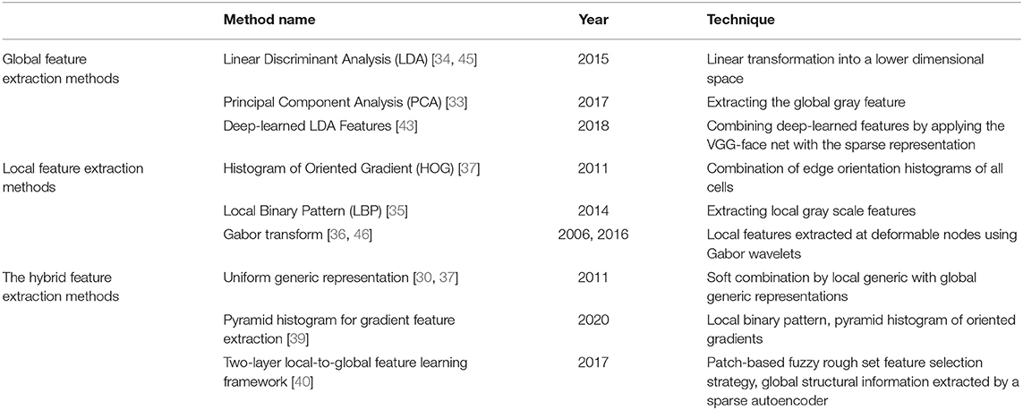
Table 2. Comparison of existing feature extraction methods.

2.3. Technical Gaps and Motivations

Although some popular methods, such as sample expansion method and feature extraction method, are proposed, they still have some shortcomings in improving the performance of SSPP recognition.

In terms of the virtual sample generation method, the above sample expansion methods can enrich the training samples, but the generated virtual samples are too similar to the original image, and the face information in the original image is insufficiently utilized, resulting in low recognition performance. Considering the advantages of NMF, this article combines NMF reconstruction theory with sample expansion methods such as mirror transformation, sliding window method, and bit plane method to propose a NMF-MSB virtual sample generation method.

In the aspect of feature extraction, the global feature is more easily affected by illumination, posture, expression, and other factors than the local feature. In recent years, researchers have found that the combination of global and local features can effectively utilize both advantages to improve recognition performance.

Histograms of Oriented Gradients method has strong adaptability to the changes of illumination, scale, and direction. This is a benefit for extracting local features of the image. WPD has the ability to eliminate redundancy and reduce image size by dimensionality reduction. Image pyramid can represent the features of a face image on multiple scales. However, local features have defects in describing the overall information of the face. Therefore, this article proposes a WPD-HOG-P feature extraction method by combining WPD, HOG, and image pyramid methods. This method embodies the combination of global and local features.

In order to verify the performance of the proposed virtual sample generation method and the WPD-HOG-P feature extraction method, an SVM model is established to realize face recognition. Experimental results show that the proposed methods have higher recognition rates and lower computational complexity compared with the benchmark methods, and the generated virtual samples can enhance the robustness of posture, expression, and illumination changes.

3. Theory Basis

We develop our theory from three aspects: sample expansion method, image reconstruction theory, and feature extraction method. The sample expansion method mainly uses the image transformation method, the sliding window method, and the bit plane method to generate virtual samples. NMF is utilized as the basic theory of image reconstruction. The feature extraction method combines HOG, WPD, and image pyramid.

3.1. Sample Expansion Method

In this article, we use three sample expansion methods—MSB methods to obtain virtual samples for enriching the sample information.

3.1.1. Mirror Transformation

Mirror transformation is a geometric transformation, which can reduce the influence of head rotation on the recognition effect to a certain extent and has little interference. There are mainly three kinds of mirror transformation methods: horizontal, vertical, and diagonal mirror methods. Figure 1A is an original image from the ORL set. Its virtual examples generated by these methods are shown in Figures 1B–D. As we can see, the transformations do not change the shape of the original image. In general, the horizontal mirror transformation can provide more abundant facial feature information than the other two methods, reflecting the possible changes of the human face to a certain extent. In this article, the horizontal mirror transformation method is used to extend the single sample face image.

FIGURE 1

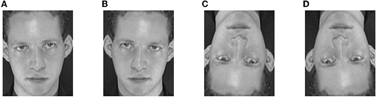
Figure 1. An original image from the ORL set and its three virtual samples generated by mirror transformation, panel (A) is an original image, panel (B) is a horizontal mirror image, panel (C) is a vertical mirror image, and panel (D) is a diagonal mirror image.

The horizontal mirroring transformation swaps the left and right halves of an image centered on the vertical center axis of the image. If the size of the original image is a × b, then the coordinate of the point (x₀, y₀) corresponding to the horizontal coordinate point in the image is (x₁, y₁). The relationship between them satisfies the following Equation (1):

$\begin{array}{ll}\{\begin{array}{c}{x}_1=a-x_0+1,\\ y_1=y_0.\end{array}& (1)\end{array}$

3.1.2. Sliding Window Method

The sliding window method selects a certain window size and a sliding step size and slides across the width and height of the image. The method is based entirely on the sample itself. It neither carries interference nor is affected by external noises. The extended sample retains and enhances the information of the original image to a large extent.

The process for the sliding window method is shown as follows: (1) Suppose the size of the sample image is a × b, the size of the sliding window is x × y, and x < a, y < b. The window starts to slide from the upper left corner of the image, and then the window can slide the length of a − x, b − y across the width and height of the sample image. (2) Set the width and height of the window to x₁, y₁, and x₁ ≤ a − x, y₁ ≤ b − y. (3) As the window slides along the width and height of the original image, a series of virtual samples can be captured from the original face image. These virtual samples constitute an extended set of the single face image. The number of window slides in the image width and height direction is n₁ and n₂. n₁ and n₂ can be calculated from Equations (2) and (3).

$\begin{array}{ll}{n}_1=\frac{a-x}{x_1}+1,& (2)\end{array}$

$\begin{array}{ll}{n}_2=\frac{b-y}{x_2}+1.& (3)\end{array}$

Take the ORL face sample in Figure 1A as an example, the image size is 92 × 112. In order to get as much information as possible, the window size needs to be set slightly larger. Let the window size be set to 84 × 104, then the width and height of the slide step are set to 8, and the number of times the window slides along the width and height can be calculated. In this case, the number of slides in both directions is 2. The window slides from the top left corner of the original image. Obviously, we can get four virtual samples. As shown in Figure 2, these samples constitute the virtual face images of the original single sample in Figure 1A.

FIGURE 2

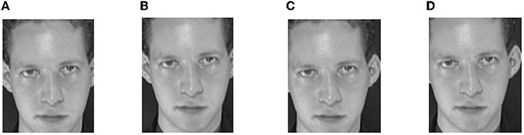
Figure 2. The virtual samples generated by sliding window method—S, Sliding window image; (A) S₁, (B) S₂, (C) S₃, and (D) S₄.

3.1.3. Bit Plane Method

Grayscale image namely refers to an 8-bit 256 color image. By extracting each bit of the image separately, we can break an image into eight images. The amount of information carried gradually decreases from the highest bit to the lowest bit. In the bit plane method, each bit can be assigned a different weight. The values on the bits with the same weight are taken out in turn to form a plane, and the image is decomposed into an 8-bit plane, as shown in Figure 3. The distribution of image information on each bit plane is different. The high-level plane contains the identifiable contour information of the image; the median plane represents the background information of the image; and the low-level plane covers the details of the image, but it is more random. Obviously, only a few higher bit plane images are visible and possess meaningful information. The original image is denoted as A, and its 8-bit plane image is denoted as A₈, A₇, A₆…A₁ in sequence. These eight images can be recombined into a series of new images according to different combination criteria. The combination formula is shown in Equation (4). By adjusting the weights of a₈ ~ a₁, different virtual samples can be generated.

$\begin{array}{ll}{A}^{\prime }={\alpha }_8*A_8+{\alpha }_7*A_7+\cdots +{\alpha }_1*A_1& (4)\end{array}$

According to different weights, the bit images are combined to obtain a series of virtual samples A′. As shown in Figure 4, the weights of these virtual samples from A′₁ to A′₆ are set to α₈ ~ α₁ =1, α₈ ~ α₂ =1,...,α₈ ~ α₆ =1, in the sequence. It can be seen that there are low and high plane combinations. These images have no obvious visual differences, indicating that the low-level plane contains little authentication information and has no significant effect on the construction of image information. In general, a new virtual sample can be constructed by selecting the middle and high-level planes.

FIGURE 3

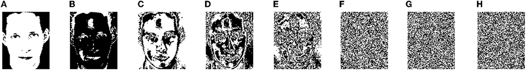
Figure 3. Decompose the original image into 8-bit planes. B, Bit plane image. (A) B₁, (B) B₂,(C) B₃, (D) B₄, (E) B₅, (F) B₆, (G) B₇, and (H) B₈.

FIGURE 4

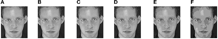
Figure 4. The virtual samples synthesized by the bit plane method. A′, Synthesized image by bit plane with different weights. (A) A′₁, (B) A′₂, (C) A′₃, (D) A′₄, (E) A′₅, and (F) A′₆.

3.2. Non-negative Matrix Factorization (NMF)

3.2.1. The Introduction of NMF Theory

The meaning of NMF is that for a non-negative matrix V, two non-negative matrices W and H are found to approximate the original matrix V [47]. In mathematical terms, given an m × n non-negative matrix V, an m × r non-negative matrix W, and an r × n non-negative matrix H are obtained, such that W and H satisfy Equation (5).

$\begin{array}{ll}V\approx WH.& (5)\end{array}$

The original matrix V can be regarded as the weighted sum of linear combinations of all column vectors in the left matrix W and the elements of all the column vectors in the right matrix H are the weight coefficients. Therefore, W is a non-negative basis matrix and H is a non-negative coefficient matrix. In addition, the value of r usually meets $r<\frac{mn}{m+n}$, so the dimensions of the matrixes W and H are less than that of the original matrix W. In this case, the original matrix V can be replaced by the coefficient matrix H, which has the effect of dimensionality reduction. The reduced dimension is also the number of non-negative basis matrices corresponding to the basis image. NMF is a partial decomposition method. For face images, the physical significance of NMF decomposition can be understood as follows: V is a matrix which is composed of n images, with m × 1 dimension; each column of the matrix represents the gray value of the face image, and the gray value of the face image is non-negative; the decomposition results are the sub-features of the image; all the sub-features constitute the overall information of the original face image.

3.2.2. The Reconstruction of Face Images With NMF Method

According to Equation (5), the non-negative matrices W and H are the approximations of the original image V. Assume that Y is the reconstructed image, which satisfies Equation (6). The degree of approximation between the reconstructed image and the original image is related to parameter r.

$\begin{array}{ll}Y=WH& (6)\end{array}$

(1) Setting for parameter r in NMF

Parameter r is not only the number of basis matrices represented by W matrix but also is the feature dimension of H matrix. Different r-values correspond to different reconstruction errors. The reconstruction error is defined as follows:

$\begin{array}{ll}Err=\frac{{\displaystyle \sum _{i,j}}|Y_{ij}-V_{ij}|}{m\times n}& (7)\end{array}$

In Equation (7), Err represents the reconstruction error, V_ij is the gray value after normalization of the original image, Y_ij is the gray value after normalization of the reconstructed image, and m × n is the size of the image. In this article, ORL and FERET face datasets are applied in the experiments. The details of both data sets are shown in Table 3. Table 4 shows the trend of NMF's average reconstruction errors as r changes on the two sets. It can be seen that with the increase of r-value, the reconstruction errors of both sets decrease. If the r-value of the two sets is equal, then the reconstruction error of the ORL set is slightly less than that of the FERET set. This is because the FERET set contains more face samples than the ORL set. The dimension of each image is also less than the ORL. The information of the image cannot be expressed by matrix effectively, and the error is also large. Hence, the best r-value for different face sets may vary. In this article, the grid optimization method is used to solve the optimal r-value.

TABLE 3

Table 3. Information of two-face sets.

TABLE 4

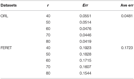
Table 4. Non-negative Matrix Factorization (NMF) reconstruction error of ORL and FERET sets.

(2) The reconstruction of the face images with NMF.

According to Equation (5), the product of the basis matrix W and the coefficient matrix H is used to obtain the reconstructed image of NMF. The initial value of r is set as 60. Parts of the original and reconstructed images from the ORL and FERET datasets are shown in Figures 5, 6, respectively. The images of the first line are the original images, and the images of the second line are the reconstructed images.

FIGURE 5

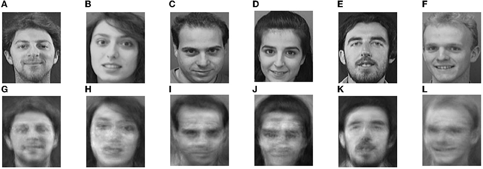
Figure 5. Part original images and their Non-negative Matrix Factorization (NMF) reconstructions in ORL, (A–F) Original ORL images, (G–L) and NMF reconstruction images.

FIGURE 6

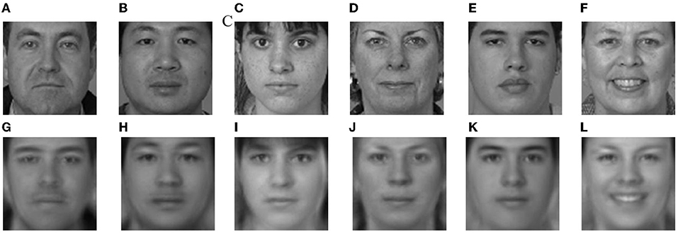
Figure 6. Part original images and their NMF reconstructions in FERET, (A–F) Original FERET images, and (G–L) NMF reconstruction images.

Comparing the original images with the reconstructed images, it can be intuitively seen that the information of the eyebrows, eyes, nose, and mouth in the reconstructed image is more prominent than the other areas. Both the base matrix W and the coefficient matrix H of NMF method are required to be non-negative, so that the weight coefficients expressed by the elements of all column vectors in H are linear combinations of all column vectors in W without subtraction. It is beneficial to image reconstruction and makes the representation of face image information more compact and less redundant.

3.3. Feature Extraction Method

3.3.1. Histograms of Oriented Gradients (HOG)

Histograms of Oriented Gradients is a feature descriptor for target detection in computer vision and image processing, which has been widely used in face recognition. HOG method also shows good performance in human gait recognition [48]. It can keep the geometric and optical changes of the image invariant. The most important advantage of this method is that the appearance and shape of local objects in the image can be well-described by the density distribution of gradient or edge.

Assume that the image has 256 × 256 pixels, divided into 16 × 16 cells. If each block is obtained by combining 2 × 2 cells, the block number (16 − 1) × (16 − 1) = 225. k is the number of uniform bins. If k is set to 9, then the features number in a block will be 2 × 2 × 9. The features number of the image is 225 × 36 = 8100 totally.

3.3.2. Wavelet Packet Decomposition

As a multi-resolution analysis method, WPD is an extension of Wavelet Transform (WT). WPD has more advantages than WT, such as non-redundancy, less computer storage, optimal time-frequency, localization, and smoothness. A WPD provides a complete wavelet packet tree, which is a signal family derived from a single mother wavelet. The corresponding scale function can subdivide the different scales of wavelet decomposition into sub-scales. WPD can adaptively select the corresponding frequency band signal according to the characteristics of the analyzed signal. It is a good decomposition method to improve the time-frequency resolution of the analyzed signal [49].

One-level WPD is performed on the original image in Figure 1A to obtain subimages A, H, V, and D, as shown in Figure 7. Among them, A is a low-frequency subimage, which reflects the contour information of the face, including most features of the face, and is most similar to the original image. H, V, and D are high-frequency subimages that include various textures of face details. These high-frequency subimages are discarded for their lower robustness to noise, expression, and light. WPD can not only achieve good results in noise reduction but also reduce the size of subimage after decomposition to a quarter of the original image, which greatly cuts down the computational complexity of feature extraction.

FIGURE 7

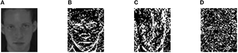
Figure 7. The Wavelet Packet Decomposition (WPD) subimages of the original image in Figure 1A. (A) A: Low-frequency subimage. (B–D) H, V, and D: high-frequency su-images.

3.3.3. Image Pyramid

An image pyramid is an efficient but simple structure that can interpret images in a variety of resolutions. An image pyramid consists of images arranged in a pyramid of diminishing resolution. The bottom of the pyramid is a high-resolution representation of the image to be processed, while the top layer is a low-resolution approximation. As one moves from the bottom of the pyramid to the top, the size and resolution of the images diminish layer by layer.

For the m × n image, sample 1:2 in the direction of rows and columns to form a (m/2) × (n/2) thumbnail image. Subsampling is repeated. With the increase of layers, the image of each layer is half of the width and height of the image below the layer, and the images of all layers constitute the pyramid [50]. The pyramid consists of three layers of images, with different resolutions. These three layers of information not only reflect the contour of the face image but also describe the details of the image. High resolution and low resolution image information constitute the multi-scale representation of the image. Multi-scale representation provides a good method for the combination of global and local features.

4. The Proposed NMF-MSB Sample Generation Method

In this article, an NMF-MSB virtual sample generation method based on sample expansion and virtual sample reconstruction is proposed. The virtual samples generated in this article include three kinds: the first kind of virtual samples are the samples A₁, A₂, and A₃ generated by mirror transformation, the sliding window method, and the bit plane method based on the original single sample A; the second kind of virtual samples A₄, A₅ are obtained by mirror transformation on the virtual samples A₂, A₃; finally, the NMF method is used to get the third kind of reconstruction virtual samples A₆, A₇, A₈, and A₉ based on the original single sample A and its first three virtual samples A₁, A₂, and A₃. Figure 8 gives the flowchart of the proposed NMF-MSB sample generation method.

FIGURE 8

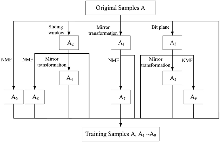
Figure 8. The flowchart of the proposed NMF-Mirror transform (M), Sliding window (S), and Bit plane (B) sample generation method.

Thus, for a single sample per person, nine virtual samples A₁ to A₉ are generated. The final training samples are composed of the original single sample and these nine virtual samples generated in this article. These samples provide more useful information for improving the recognition performance of SSPP. Figures 9, 10 give an original image and its nine virtual samples of ORL and FERET face sets generated by the above-mentioned methods.

FIGURE 9

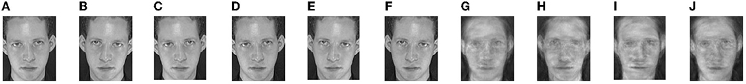
Figure 9. An original image and its 9 virtual samples of ORL set. (A) An original image and (B–J) its 9 virtual samples.

FIGURE 10

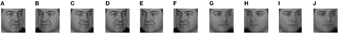
Figure 10. An original image and its 9 virtual samples of FERET set. (A) An original image and (B–J) its 9 virtual samples.

Mirror transformation, sliding window, and bit plane methods are three typical sample expansion methods. Each method has its own unique advantages. NMF is a good face image reconstruction method. It can better express the internal relationship between the local features of the face. This is beneficial to further improve the recognition performance of SSPP. Mirror transformation can eliminate the influence of local rotation on recognition performance. The sliding window method can better simulate the position relationship and distance between the lens and face during image sampling. The bit plane method gives the possible changes of the pixel to some extent. Each method has its own advantages. It is helpful for improving the robustness to changes of facial posture, expression, and illumination. The NMF reconstruction method is non-negative and makes the depiction of human face information more effective. NMF reconstruction based on face images can provide more detailed feature information of face samples.

5. The Proposed WPD-HOG-P Feature Extraction Method

A WPD-HOG-P feature extraction method is proposed in this article. This method combines the advantages of WPD and HOG features and adopts a multi-scale pyramid model. The subimages at each scale have different resolutions. The face image set is decomposed and the low-frequency subimages are down sampled two times to obtain the multi-scale subimages. It is useful to extract key information at different resolutions. In addition, the method eliminates the high-frequency subimages and improves the computational performance.

The WPD-HOG-P feature extraction process proposed in this article is shown in Figure 11. The pseudocode of the WPD-HOG-P feature extraction method is shown in Algorithm 1. First, the WPD is performed to set E for getting low-frequency subimage set Im_A; then sampling two times at a sub-sampling rate of 1:2 at an interval of 1 pixel to get the image pyramid P{P₁, P₂, P₃}. In the pyramid, it contains subimages of three different resolutions. For the subimages of all layers, HOG features are calculated according to the procedure of the HOG feature extraction method introduced in section 3.3.1. Lastly, all HOG features H₁, H₂, and H₃ of each layer in the image pyramid are concatenated together to form the final WPD-HOG-P features.

FIGURE 11

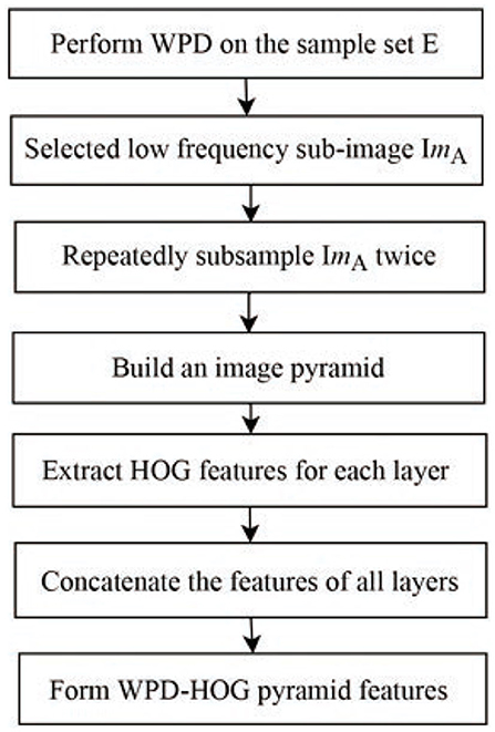
Figure 11. The flowchart of Wavelet Packet Decomposition, Histograms of Priented Gradients, and image Pyramid feature extraction method.

ALGORITHM 1

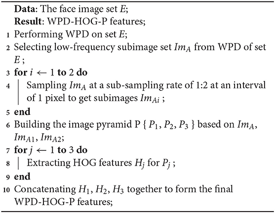
Algorithm 1: The pseudocode of WPD-HOG-P feature extraction method.

A 64 × 80 face image is taken as an example to illustrate the process of WPD-HOG-P feature extraction. Here, the number of bins k is set to 9, cell = 4 × 4, each 2 × 2 cell forms a block, since each cell has 9 features, so there are 4 × 9 = 36 features in each block, and the width of a cell is the overlap between adjacent blocks, therefore, the step size is 4 pixels.

The feature extraction process of the WPD-HOG-P method proposed in this article is as follows: first, the image is processed by WPD to get 4 subimages of 32 × 40 size, and then three high-frequency subimages are discarded. The low-frequency subimages are subsampled to obtain 16 × 20 and 8 × 10 size subimages, respectively. For three layers of the pyramid, the HOG feature is extracted from each layer of images. For an image of size 32 × 40, there would be (32/4) − 1 = 7 scan windows in the horizontal direction and (40/4) − 1 = 9 scan windows in the vertical direction, i.e., 7 × 9 image blocks. The three-layer image pyramid is characterized by the size of 36 ×7 × 9, 36 × 3 × 4, and 36 × 1 × 1, respectively. Finally, the features of the three-layer images are connected in series to obtain the WPD-HOG-P features, whose size is 36 × 7 × 9 + 36 × 3 × 4 + 36 × 1 × 1 = 2736.

The traditional HOG feature extraction method utilizes the entire face image to extract local features information and achieves single-scale image expression. It contains a lot of redundant information that is not favorable to the recognition of face images but increases the computational complexity. For example, if the HOG features are extracted from the original image with the size of 64 × 80 face images, there are a total of 36 × 15 × 19 = 10, 260 dimensional features. Apparently, 10,260 is much bigger than 2,736. It means that the features number of the traditional HOG feature extraction method is much bigger than the number of WPD-HOG-P features, which greatly increases the computational complexity. Moreover, because the traditional HOG feature extraction method only contains single-scale image information, the features extracted cannot fully express the information of the face image.

6. Experiments

6.1. Face Data Sets Introduction

In this article, ORL and FERET face sets are used for experiments. Details of both sets are shown in Table 3.

The ORL face set is one of the most widely used face sets, consisting of 40 objects of different ages, genders and races. There are 400 grayscale images, 10 images per person, image grayscale of 256, image size of 92 × 112. It also includes images of different facial expressions, facial accessories, lights, and poses. The change of the face is also within 20%. In the experiment, one of each person's 10 images is chosen as a training sample. The experiment is repeated 10 times. Each time, a different sample from each person is used as a training sample, and the remaining 9 images are used as test samples. Therefore, the training set contains 40 original samples and the test set contains 360 samples.

FERET face set selects 200 categories of objects, 7 images per person, a total of 1,400. In the experiments, only one sample per person is selected each time. The first frontal face image of each person is selected as the training sample, and the other 6 images belong to the test sample. Where, the 2 − 5th images per person are the images changing posture, denoted as Test₁; the 6th image per person is the image that changes the expression, recorded as Test₂; the 7th image per person is the image that changes the lighting and is recorded as Test₃, as shown in Table 5.

TABLE 5

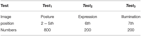
Table 5. Information of FERET set.

Therefore, the original training set A contains a total of 200 samples, the test set Test₁ has 800 samples, Test₂ has 200 samples, and Test₃ has 200 samples. The frontal face images of 200 people and their virtual samples constitute a training set of 2,000 samples E.

6.2. Experimental Design

The recognition performance is quantitatively evaluated by the criterion of recognition rate. The feature dimension and time consumption are used to evaluate the performance of computational complexity quantitatively. The experiments are repeated 10 times. Each result is an average of 10 times.

6.2.1. WPD-HOG Pyramid Feature Extraction Method

The proposed feature extraction method (marked as “WPD-HOG-P”) is compared with the following three methods for the effectiveness and noise robustness of face feature extraction.

(1) Benchmark 1: HOG feature. The traditional HOG feature extraction method in [51] is the first benchmark.

(2) Benchmark 2: HOG pyramid(HOG-P) feature. The HOG and image pyramid face recognition method proposed in [40] is adopted as the second benchmark. First, an image pyramid is built on the images, and then the HOG features of all images in the pyramid are extracted. Finally, these HOG features are concatenated together as the final features of the HOG pyramid benchmark method.

(3) Benchmark 3: Convolutional Neural Network (CNN). CNN can extract the deep features of the image. Here, the CNN model includes two convolution layers and two sub-sampling layers. Softmax function is adopted in the output layer and 200 epochs are used to train the model.

In addition, in order to verify the noise robustness of the proposed feature extraction method, some different types of noise are added in the SSPP condition. There are two kinds of noise: one is salt and pepper noise, and the other is Gaussian white noise. In this experiment, salt and pepper have a noise intensity of 0.1. There are two Gaussian white noises with zero mean and 0.01 and 0.1 variance respectively. One type of noise is added to the ORL face image each time.

6.2.2. Virtual Sample Generation

In this article, the virtual samples are generated based on the fusion of the NMF reconstruction method and three sample expanding methods. The virtual samples generation procedure is given in Section 4.

First, the performance comparison of virtual sample reconstruction method based on NMF with different dimension r is studied on ORL and FERET sets.

Then, the proposed virtual sample generation method (marked as “NMF-MSB”) is compared with the following four methods.

(1) Original: The training sample set is not extended. Feature extraction and recognition are carried out directly on this set. It is recorded as “original” in the experiments.

(2) Mirroring: The virtual sample by mirror transformation, marked as A₁, and original sample A are combined to form a new training set B = {A, A₁}. It is recorded as “Mirror” in the experiments.

(3) Sliding Window: The virtual sample by sliding window, marked as A₂, are combined with A to form a new training set C = {A, A₂}. It is recorded as “Window” in the experiments.

(4) Bit plane: A similar method is used to obtain the training set D = {A, A₃}, where A₃ is generated by bit plane method. It is recorded as “Bit.”

6.3. The Experiment of Feature Extraction Method

(1) The recognition performance of the proposed WPD-HOG-P feature extraction method.

A comparison of the recognition rates between our method and the benchmark methods under four different noise conditions is shown in Figure 12. It can be seen that, except Noise 2, the recognition rates of our WPD-HOG-P feature extraction methods are generally higher than that of the three benchmark methods. The recognition rate of our method is over 60% without noise, which is improved by 8.5% compared to the HOG method, by 6.03% to the HOG-P method, and a little less than the CNN method. In Noise 1 situation, the recognition rate of our method is improved by 11.63% compared to the HOG method, by 5.75% to the HOG-P method, and by 6.98% to the CNN method. In Noise 2 situation, the recognition performance of our method is better than HOG and HOG-P methods, but poor than CNN.

FIGURE 12

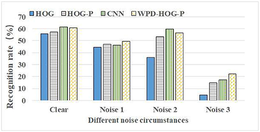
Figure 12. The recognition rate comparison of WPD-HOG-P with benchmark methods in Single Sample Per Person (SSPP). WPD-HOG-P, the proposed feature extraction method. Clear, no noise. Noise 1, salt and pepper noise. Noise 2, Gaussian noise 1 (variance is 0.01). Noise 3, Gaussian noise 2 (variance is 0.1).

The reasons why our feature extraction method is superior to the three benchmark methods are as follows: (1) HOG method only extracts local features of the image, while our WPD-HOG-P feature is a multi-scale representation of the image, which combines global and local features. It makes the extracted features have stronger description ability and more abundant feature information to face image. (2) Compared with the HOG pyramid method, our method first uses WPD to preprocess the image and remove interference information such as noise, light, and expression change. It makes feature expressions more compact. This is beneficial to improve recognition performance.

(2) Noise robustness of proposed WPD-HOG-P feature extraction method

Under the attack of salt and pepper noise, the recognition rates of the proposed feature extraction method in this article are compared in the case of “Noise 1” under three benchmarks, as shown in Figure 12. The results show that the WPD-HOG-P feature extraction method proposed in this article has the highest recognition rate among the four methods. Compared with HOG, HOG pyramid, and CNN, the recognition rates of the proposed method under salt and pepper noise attack are increased by 11.63, 5.75, and 6.98%, respectively.

Under the attack of Gaussian noise, the recognition rates of our method and three benchmark methods are compared as shown in Figure 12 in the cases of “Noise 2” and “Noise 3.” Obviously, under different Gaussian noise conditions, the recognition rates obtained by our method are all higher than those obtained by three benchmark methods except the CNN method in the case of “Noise 2.” When the Gaussian noise variance is 0.01, the improvement of the recognition rate of the proposed method than HOG and HOG-P methods is about 56.67 and 5.35%, but less than CNN about 5.59%. When the variance is 0.1, the recognition rate of our feature method is about 22.21%, which is much higher than the three benchmarks.

To sum up, HOG features are easily disturbed by noise. Our feature extraction method greatly improves the feature's anti-noise performance due to the use of WPD for denoising. In addition, our feature extraction method removes high-frequency sub-images susceptible to noise after WPD. Moreover, the multi-scale representation of the image pyramid enhances the noise resistance of the features.

6.4. The Experiment of NMF Virtual Sample Generation Method

6.4.1. The Influence of r-Value on Recognition Rate

The influence of different r-values on the recognition rate in using NMF for ORL and FERET sets is studied in this subsection. The goal is to find the best r-value for the two face sets, respectively.

(1) The setting of parameter r on ORL set

In using the NMF reconstruction method on the ORL set, parameter r is set from 10 to 80 with step 10 during reconstruction. The average recognition rate and time consumption comparisons of different r are shown in Figure 13. It can be seen that the best average recognition rate is r = 50. The rates are more than 68% when r is 40, 50, 70, and 80. Apparently, the time consumption gradually increases when the value r increases. Therefore, to ensure recognition performance, the r-value needs to be set to an appropriate value. In this article, it is set to r = 50.

(2) The setting of parameter r on FERET set

FIGURE 13

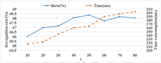
Figure 13. The recognition rate and time consumption comparisons of different r on ORL.

ORL face set only contain 40 objects, but FERET set contains 200 objects. It is much more than the number in ORL set. It means the best value of r on FERET set should be much bigger than on ORL set for getting prominent reconstruction images. The initial r-value on FERET is set to 100. Then, the value of r is adjusted from 100 to 500 with a step of 100.

The test sets of FERET include 3 different kinds (see section 6.1). The recognition rate and time consumption comparisons are shown in Figure 14, where Av₋R means the average recognition rate of 3 test sets. The left vertical axis represents the recognition rate and the right vertical axis represents time consumption. Time consumption is obtained on the environment with Intel(R) Core (TM) i5-2520M CPU, 6GB RAM, Win7 OS, and MATLAB R2015b software. As we can see, the rate is best when the r parameter is set to 400. Similarly, as r increases, so does the time consumption.

FIGURE 14

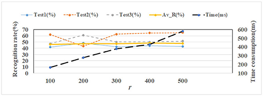
Figure 14. The recognition rate and time consumption comparisons of different r on FERET.

6.4.2. Analysis and Discussion

Based on the above experimental results on both sets, we can see that the virtual sample generation method based on NMF reconstruction theory has the following characteristics:

(1) The recognition rates of both sets increase with an increase in r. However, when r is large enough, the recognition rates decrease. This is because when the r-value is too small, the reconstructed image contains too little face information, which cannot effectively represent the face image; if the r-value is too large, the reconstructed image contains too much redundant information and auxiliary interference. Therefore, the value of r should be set to an appropriate value.

(2) The more samples the face set contains, the larger the r-value is. It can be seen that, for the ORL set with the sample size of 400, the optimal value is r=50. For the FERET set with the sample size of 1,400, the optimal r-value is 400. This is because NMF is performed on all samples in the training set. Feature extraction is closely related to all training samples, and these samples are not independent. Therefore, when the number of training samples increases, the optimal r-value also increases accordingly.

(3) The larger the r-value is, the more time it takes to reconstruct the image. It can be seen from the experimental results in Figures 13, 14 that the image reconstruction time increases with an increase in r-value. In image reconstruction, r is the number of base images of the non-negative matrix W, that is, the feature dimension of H. The larger the r-value is, the more complex and time-consuming the image reconstruction will be.

6.5. Experiments on Proposed NMF-MSB Virtual Sample Generation Method

The recognition rate comparison between the proposed NMF-MSB virtual sample generation method and the benchmark methods on the ORL set is shown in Figure 15. It can be seen that the proposed NMF-MSB method has a better recognition rate than all the benchmark methods. The mirror transformation method is the second-best of all, with a recognition rate of about 66%. The recognition rates based on original, sliding window, and bit plane methods are close to each other. The grid search method is further used to adjust the SVM classifier parameters of all methods except the original set, and the cross-validation method is used to reduce the overfitting of the model. It can be seen that, compared with the non-optimized SVM, the recognition rate of our NMF-MSB method is improved by about 5%, still maintaining the best recognition rate, and the mirror transformation method still is the second best.

FIGURE 15

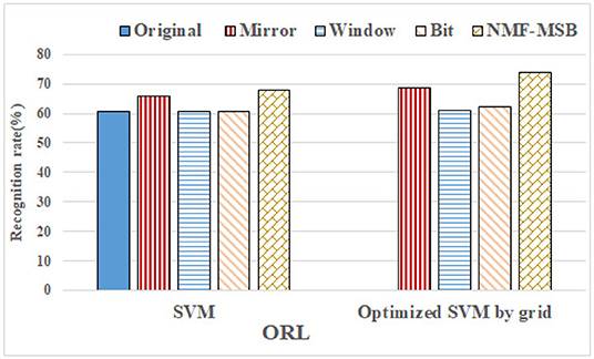
Figure 15. The recognition rate comparison of the NMF-MSB method with benchmark methods on ORL.

For the FERET dataset, the recognition rate comparison between the proposed NMF-MSB virtual sample generation method and the benchmark methods is shown in Figure 16. We can see that the recognition rate of the proposed NMF-MSB virtual sample generation method is about 2–11% higher than that of the benchmark methods, before grid search optimization of SVM. Compared with non-optimized SVM, the recognition rate of Mirror, Window, and Bit methods are improved by less than 1%, and the optimization effect is not significant. The proposed NMF-MSB virtual sample generation method improves the recognition rate by about 5% because it has more training samples. The performance of the proposed virtual sample generation method is verified.

FIGURE 16

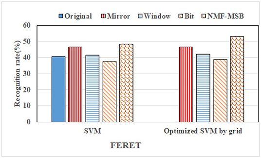
Figure 16. The recognition rate comparison of the NMF-MSB method with benchmark methods on FERET.

From the experimental results of ORL and FERET face data sets, it can be seen that the proposed method combined the advantages of three sample expansion methods: mirror transformation, window sliding, and bit plane. It is beneficial to improve the robustness of the virtual samples to the changes of posture, expression, and illumination. The virtual samples generated by sliding window and bit plane methods are further dealt with mirror transformation. The images after mirror transformation contain more information than the original single sample image so that the original sample information can be fully utilized. The non-negative constraint of NMF enhances the representation ability of face image. By setting an appropriate r-value, NMF makes the face information contained in the reconstructed image more compact and less redundant, which lays a good foundation for subsequent feature extraction and recognition.

6.6. Non-parametric Tests

The non-parametric test is a statistical test that makes weaker assumptions about data distribution than tests based on normal distribution or other statistical tests such as t-test. Non-parametric tests are performed in this subsection to reveal the statistical differences between our method and benchmark methods.

The Wilcoxon test and Friedman test are two typical non-parametric tests [52]. They are utilized in our experiments. For the Wilcoxon test, the Wilcoxon sign rank test is mainly concerned.

The initial hypothesis of all tests is that “There is no significant difference in the overall distribution between the two methods.” Wilcoxon signed rank test can give h and p-values to test the difference between the two methods, where p-value represents the probability that the two median values are equal. If p-value is close to 0, the initial hypothesis is called into question. In this case, the difference between the two methods is significant and the hypothesis can be rejected. If h = 0, it indicates that the difference between the two methods is not significant; otherwise, h = 1 indicates a large difference between the two methods. For the Friedman test, if the p-value is less than 0.05, then the initial hypothesis is invalid, otherwise, it means the original hypothesis is valid. Table 6 shows the test results of our methods and benchmark methods.

TABLE 6

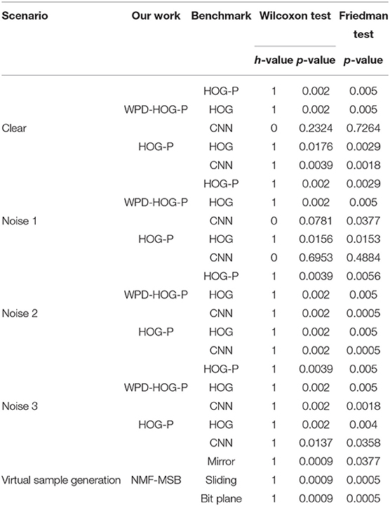
Table 6. Results of Wilcoxon and Friedman tests.

As can be seen, the p values of the results tested by the two methods are both very low, indicating that our WPD-HOG-P feature extraction method is significantly different from all the benchmark feature extraction methods. The recognition performance of the WPD-HOG-P feature extraction method is close to CNN for both p = 0.2324 and h = 0, and the result of Friedman is much more than 0.05. We can get similar results from Figure 12.

We also compare the differences of HOG-P with CNN and HOG methods. The results mean that, compared to HOG-P and CNN methods, the HOG feature extraction method also has significant differences with them in face recognition performance. However, in Noise 1, the p-values between HOG-P and CNN in the two tests are far greater than 0.05, indicating that there is no significant difference between the two methods in this case.

7. Conclusion

In this article, sample expansion and feature extraction methods are addressed for solving the SSPP challenge. For sample expansion method, this article proposes an NMF-MSB virtual samples generating method which combines mirror transformation, sliding window, and bit plane methods as well as NMF. For the feature extraction method, this article proposes a WPD-HOG-P method that combines WPD, HOG feature, and image pyramid methods together to effectively represent face images. Experimental results on ORL and FERET face sets show that the proposed NMF-MSB method not only makes full use of the traditional advantages of three sample expansion methods but also improves the robustness of face to the pose, expression, and illumination changes by combining with the NMF reconstruction method. The improvement of recognition rate and the reduction of time computation verify the good advantages of the proposed WPD-HOG-P feature extraction method.

However, the proposed methods still have some shortcomings. While enriching the training samples, the computational complexity will also increases especially when the size of the face set is large, it will take a lot of time. Moreover, the recognition rates of all experiments are not so high enough. The reason is that this article mainly studies the generation of virtual samples and feature extraction methods, but does not carry out model optimization, which is also the main aspect to improve the recognition performance. This paper only uses the classical support vector machine algorithm to construct the recognition model, and does not study its optimization strategy for face recognition.

Data Availability Statement

The original contributions presented in the study are included in the article/supplementary material, further inquiries can be directed to the corresponding author/s.

Author Contributions

FL has contributed to write the manuscript and share the first authorship. TY has contributed to perform the experiment. YZ has contributed to perform the analysis with constructive discussions. WL has contributed to perform the manuscript preparation. All authors contributed to the article and approved the submitted version.

Funding

This work was supported in part by the National Natural Science Foundation of China (NSFC) under Grant 62171307.

Conflict of Interest

The authors declare that the research was conducted in the absence of any commercial or financial relationships that could be construed as a potential conflict of interest.

Publisher's Note

All claims expressed in this article are solely those of the authors and do not necessarily represent those of their affiliated organizations, or those of the publisher, the editors and the reviewers. Any product that may be evaluated in this article, or claim that may be made by its manufacturer, is not guaranteed or endorsed by the publisher.

References

1. Jindal A, Gupta S, Kaur L. Face recognition techniques with permanent changes: a review. In: International Conference on Green Computing and Internet of Things. Greater Noida (2016). doi: 10.1109/ICGCIoT.2015.7380551

PubMed Abstract | CrossRef Full Text | Google Scholar

2. Taskiran M, Kahraman N, Erdem CE. Face recognition: past, present and future (a review). Digit Signal Process. (2020) 106:102809. doi: 10.1016/j.dsp.2020.102809

CrossRef Full Text | Google Scholar

3. Xu Y. Single sample face recognition based on sample augments and MSD fusion. In: 2016 IEEE Information Technology, Networking, Electronic and Automation Control Conference. Chongqing: IEEE (2016). p. 352–5.

Google Scholar

4. Zhuang L, Yang AY, Zhou Z, Shankar Sastry S, Ma Y. Single-sample face recognition with image corruption and misalignment via sparse illumination transfer. In: Proceedings of the IEEE Conference on Computer Vision and Pattern Recognition. (2013) p. 3546–53. doi: 10.1109/CVPR.2013.455

CrossRef Full Text | Google Scholar

5. Pei T, Li Z, Wang B, Li F, Zhao Z. Decision Pyramid Classifier for face recognition under complex variations using single sample per person. Pattern Recogn. (2017) 64:305–13. doi: 10.1016/j.patcog.2016.11.016

CrossRef Full Text | Google Scholar

6. Lei Y, Guo Y, Hayat M, Bennamoun M, Zhou X. A Two-Phase Weighted Collaborative Representation for 3D partial face recognition with single sample. Pattern Recogn. (2016) 52:218–37. doi: 10.1016/j.patcog.2015.09.035

CrossRef Full Text | Google Scholar

7. Ji HK, Sun QS, Ji ZX, Yuan YH, Zhang GQ. Collaborative probabilistic labels for face recognition from single sample per person. Pattern Recogn. (2017) 62:125–34. doi: 10.1016/j.patcog.2016.08.007

CrossRef Full Text | Google Scholar

8. Zhang D, Lv C, Liu N, Wu Z, Wang X. 3D face modeling from single image based on discrete shape space. Comput Animat Virtual Worlds. (2020) 31:4–5. doi: 10.1002/cav.1943

CrossRef Full Text | Google Scholar

9. Wang X, Zhang B, Yang M, Ke K, Zheng W. Robust joint representation with triple local feature for face recognition with single sample per person. Knowledge Based Syst. (2019) 181:1–16. doi: 10.1016/j.knosys.2018.11.011

CrossRef Full Text | Google Scholar

10. Wang H, Zhang DS, Miao ZH. Face recognition with single sample per person using HOG-LDB and SVDL. Signal Image Video Process. (2019) 13:985–92. doi: 10.1007/s11760-019-01436-1

CrossRef Full Text | Google Scholar

11. Choi SI, Lee Y, Lee M. Face recognition in SSPP problem using face relighting based on coupled bilinear model. Sensors. (2018) 19:43. doi: 10.3390/s19010043

PubMed Abstract | CrossRef Full Text | Google Scholar

12. Hong S, Im W, Ryu J, Yang HS. SSPP-DAN: Deep domain adaptation network for face recognition with single sample per person. In: 2017 IEEE International Conference on Image Processing (ICIP). Beijing (2017). p. 825–9. doi: 10.1109/ICIP.2017.8296396

CrossRef Full Text | Google Scholar

13. Liu F, Wang F, Ding Y, Yang S. SOM-based binary coding for single sample face recognition. J Ambient Intell Human Comput. (2021). doi: 10.1007/s12652-021-03255-0. [Epub ahead of print].

CrossRef Full Text | Google Scholar

14. Meng Y, Xing W, Zeng G, Shen L. Joint and collaborative representation with local adaptive convolution feature for face recognition with single sample per person. Pattern Recogn. (2016) 66:117–28. doi: 10.1016/j.patcog.2016.12.028

CrossRef Full Text | Google Scholar

15. Adjabi I, Ouahabi A, Benzaoui ea A. Multi-block color-binarized statistical images for single-sample face recognition. Sensors. (2021) 21:728. doi: 10.3390/s21030728

PubMed Abstract | CrossRef Full Text | Google Scholar

16. Zhang T, Li X, Guo RZ. Producing virtual face images for single sample face recognition. Int J Light Electron Optics. (2014) 125:5017–24. doi: 10.1016/j.ijleo.2014.01.171

CrossRef Full Text | Google Scholar

17. Lee J, Bang J, Yang SI. Object detection with sliding window in images including multiple similar objects. In: International Conference on Information and Communication Technology Convergence. Hangzhou (2017). p. 803–6. doi: 10.1109/ICTC.2017.8190786

CrossRef Full Text | Google Scholar

18. Schlett T, Rathgeb C, Busch C. Deep learning-based single image face depth data enhancement. Comput Vision Image Understand. (2021) 210:2502–15. doi: 10.1016/j.cviu.2021.103247

CrossRef Full Text | Google Scholar

19. Song F, Yong X, Zhang D, Liu T. A novel subspace-based facial discriminant feature extraction method. In: Chinese Conference on Pattern Recognition (CCPR). Nanjing (2009). doi: 10.1109/CCPR.2009.5343963

PubMed Abstract | CrossRef Full Text | Google Scholar

20. Wang X, Zhang B, Yang M, Ke K, Zheng W. Robust joint representation with triple local feature for face recognition with single sample per person. Knowledge Based Syst. (2019) 181:104790. doi: 10.1016/j.knosys.2019.05.033

CrossRef Full Text | Google Scholar

21. Min R, Xu S, Cui Z. Single-sample face recognition based on feature expansion. IEEE Access. (2019) 7:45219–29. doi: 10.1109/ACCESS.2019.2909039

CrossRef Full Text | Google Scholar

22. Goyal A, Meenpal T. Robust discriminative feature subspace analysis for kinship verification. Inform Sci. (2021) 578:507–24. doi: 10.1016/j.ins.2021.07.046

CrossRef Full Text | Google Scholar

23. Chen WS, Yang Z, Pan B, Bo C. Supervised kernel nonnegative matrix factorization for face recognition. Neurocomputing. (2016) 205:165–81. doi: 10.1016/j.neucom.2016.04.014

CrossRef Full Text | Google Scholar

24. Lu Y, Lai Z, Xu Y, You J, Li X, Yuan C. Projective robust nonnegative factorization. Inform Sci. (2016) 364–365:16–32. doi: 10.1016/j.ins.2016.05.001

CrossRef Full Text | Google Scholar

25. Pang M, Cheung YM, Wang B, Liu R. Robust heterogeneous discriminative analysis for face recognition with single sample per person. Pattern Recogn. (2019) 89:91–107. doi: 10.1016/j.patcog.2019.01.005

CrossRef Full Text | Google Scholar

26. Hu X, Peng S, Wang L, Yang Z, Li Z. Surveillance video face recognition with single sample per person based on 3D modeling and blurring. Neurocomputing. (2017) 235:46–58. doi: 10.1016/j.neucom.2016.12.059

CrossRef Full Text | Google Scholar

27. Yu C, Zhang Z, Li H. Reconstructing a large scale 3D face dataset for deep 3D face identification. arXiv preprint arXiv:2010.08391. (2020).

Google Scholar

28. Xiao H, Yu W, Jing Y. Multi-oriented 2DPCA for face recognition with one training face image per person. J Comput Inform Syst. (2010).

Google Scholar

29. Yang M, Wang X, Zeng G, Shen L. Joint and collaborative representation with local adaptive convolution feature for face recognition with single sample per person. Pattern Recogn. (2016) 66:117–28.

Google Scholar

30. Ding Y, Liu F, Tang Z, Zhang T. Uniform generic representation for single sample face recognition. IEEE Access. (2020) 8:158281–92. doi: 10.1109/ACCESS.2020.3017479

CrossRef Full Text | Google Scholar

31. Tan X, Chen S, Zhou ZH, Zhang F. Face recognition from a single image per person: a survey. Pattern Recogn. (2006) 39:1725–45. doi: 10.1016/j.patcog.2006.03.013

CrossRef Full Text | Google Scholar

32. De A, Saha A, Pal MC. A human facial expression recognition model based on eigen face approach. Proc Comput Sci. (2015) 45:282–9. doi: 10.1016/j.procs.2015.03.142

CrossRef Full Text | Google Scholar

33. Turhan CG, Bilge HS. Class-wise two-dimensional PCA method for face recognition. IET Comput Vis. (2017) 11:286–300. doi: 10.1049/iet-cvi.2016.0135

CrossRef Full Text | Google Scholar

34. Ghassabeh YA, Rudzicz F, Moghaddam HA. Fast incremental LDA feature extraction. Pattern Recogn. (2015) 48:1999–2012. doi: 10.1016/j.patcog.2014.12.012

CrossRef Full Text | Google Scholar

35. Jia M, Zhang Z, Song P, Du J. Research of improved algorithm based on LBP for face recognition. Lecture Notes Comput Sci. (2014) 8833:111–9. doi: 10.1007/978-3-319-12484-1_12

CrossRef Full Text | Google Scholar

36. Karthika R, Parameswaran L. Study of Gabor wavelet for face recognition invariant to pose and orientation. In: Proceedings of the International Conference on Soft Computing Systems. Springer (2016). p. 501–9. doi: 10.1007/978-81-322-2671-0_48

CrossRef Full Text | Google Scholar

37. Déniz O, Bueno G, Salido J, Torre FDL. Face recognition using histograms of oriented gradients. Pattern Recogn Lett. (2011) 32:1598–603. doi: 10.1016/j.patrec.2011.01.004

CrossRef Full Text | Google Scholar

38. Karanwal S, Diwakar M. Neighborhood and center difference-based-LBP for face recognition. Pattern Anal Appl. (2021) 24:741–61. doi: 10.1007/s10044-020-00948-8

CrossRef Full Text | Google Scholar

39. Sharifnejad M, Shahbahrami A, Akoushideh A, Hassanpour RZ. Facial expression recognition using a combination of enhanced local binary pattern and pyramid histogram of oriented gradients features extraction. IET Image Process. (2021) 15:468–78. doi: 10.1049/ipr2.12037

CrossRef Full Text | Google Scholar

40. Guo Y, Jiao L, Wang S, Liu F. Fuzzy sparse autoencoder framework for single image per person face recognition. IEEE Trans Cybernet. (2017) 48:2402–15. doi: 10.1109/TCYB.2017.2739338

PubMed Abstract | CrossRef Full Text | Google Scholar

41. LeCun Y, Bengio Y, Hinton G. Deep learning. Nature. (2015) 521:436–44. doi: 10.1038/nature14539

PubMed Abstract | CrossRef Full Text | Google Scholar

42. Zeng J, Zhao X, Gan J, Mai C, Zhai Y, Wang F. Deep convolutional neural network used in single sample per person face recognition. Comput Intell Neurosci. (2018) 2018:3803627. doi: 10.1155/2018/3803627

PubMed Abstract | CrossRef Full Text | Google Scholar

43. Bodini M, D'Amelio A, Grossi G, Lanzarotti R, Lin J. Single sample face recognition by sparse recovery of deep-learned LDA features. In: International Conference on Advanced Concepts for Intelligent Vision Systems. Espace Mendes; Poitiers: Springer (2018). p. 297–308. doi: 10.1007/978-3-030-01449-0_25

CrossRef Full Text | Google Scholar

44. Tewari A, Zollhoefer M, Bernard F, Garrido P, Kim H, Perez P, et al. High-fidelity monocular face reconstruction based on an unsupervised model-based face autoencoder. IEEE Trans Pattern Anal Mach Intell. (2018) 42:357–70. doi: 10.1109/TPAMI.2018.2876842

PubMed Abstract | CrossRef Full Text | Google Scholar

45. Tang EK, Suganthan PN, Yao X, Qin AK. Linear dimensionality reduction using relevance weighted LDA. Pattern Recogn. (2005) 38:485–93. doi: 10.1016/j.patcog.2004.09.005

PubMed Abstract | CrossRef Full Text | Google Scholar

46. Shen BL L. A review on Gabor wavelets for face recognition. Pattern Anal Appl. (2006) 9:273–92. doi: 10.1007/s10044-006-0033-y

CrossRef Full Text | Google Scholar

47. Yu D, Chen N, Jiang F, Fu B, Qin A. Constrained NMF-based semi-supervised learning for social media spammer detection. Knowledge Based Syst. (2017) 125:64–73. doi: 10.1016/j.knosys.2017.03.025

CrossRef Full Text | Google Scholar

48. Anusha R, Jaidhar CD. Human gait recognition based on histogram of oriented gradients and Haralick texture descriptor. Multimedia Tools Appl. (2020) 79:8213–234. doi: 10.1007/s11042-019-08469-1

CrossRef Full Text | Google Scholar

49. Zhang Y, Ji X, Zhang Y. Classification of EEG signals based on AR model and approximate entropy. In: International Joint Conference on Neural Networks. (2015). doi: 10.1109/IJCNN.2015.7280840

CrossRef Full Text | Google Scholar

50. Lai WS, Huang JB, Ahuja N, Yang MH. Deep Laplacian pyramid networks for fast and accurate super-resolution. In: 2017 IEEE Conference on Computer Vision and Pattern Recognition (CVPR). Honolulu, HI; Hawaii (2017). doi: 10.1109/CVPR.2017.618

PubMed Abstract | CrossRef Full Text | Google Scholar

51. Sun M, Li D. Smart face identification via improved LBP and HOG features. Internet Technol Lett. (2020) e229:1–6. doi: 10.1002/itl2.229

CrossRef Full Text | Google Scholar

52. Demšar J. Statistical comparisons of classifiers over multiple data sets. J Mach Learn Res. (2006) 7:1–30. doi: 10.1007/s10846-005-9016-2

CrossRef Full Text | Google Scholar