Modeling dynamics of adult female lice at salmon farming sites in Eastern Canada: a stochastic, state-based approach

Introduction: Sea lice are parasitic copepods that harm salmon health, reduce farm productivity, and create ecological and economic challenges for aquaculture.

Methods: A stochastic, state-based, time-dependent epidemiological model was developed to characterize the dynamics of adult female sea lice (Lepeophtheirus salmonis) infestation in Atlantic salmon farms in New Brunswick, Canada. The model integrated covariates associated with farming practices and environmental conditions (stocking week, farming cycle week as proxy of fish age, sea lice treatments, seaway distance to neighboring farms as a proxy for waterborne transmission, and sea surface temperature). Data from 57 farming sites were used for model training and validation. An initial exploratory analysis assessed the relationship between treatment timing and recovery from infestation. Treatment effects were incorporated into weekly transitions between infestation states, accounting for severity and time-varying environmental factors.

Results: Results suggest that spring and summer stocking increases exposure to external infestation pressure and raises the probability of high lice concentrations. Further, reduced winter treatments are associated with elevated infestation levels. Treatment effectiveness appeared to be compromised by continued waterborne transmission from nearby farms.

Discussion: The model achieved an overall likelihood of 59%, reaching up to 74% during the first 10 weeks following stocking. Limitations included the use of proxy connectivity measures, i.e. seaway distance, rather than hydrodynamic connectivity, and the absence of data on fish size, salinity, and other farming practices such as fish density. Additionally, we were unable to include information from all farms in the study area, potentially underestimating transmission risk. Addressing these gaps and integrating hydrodynamic connectivity and fish growth models could improve predictive performance.

1 Introduction

Sea lice (Lepeophtheirus salmonis and Caligus sp.) are ectoparasitic copepods that negatively impact the welfare and health of salmon and may lead to reduced productivity and economic losses in farms (Costello, 2009; Abolofia et al., 2017). Lepeophtheirus salmonis is present in areas such as the southeastern coast of New Brunswick, Canada, where Atlantic salmon farming contributes to the regional economy with an estimated production of 9,593 tons of salmon and 73.7 CAD million dollars in 2022 (Government of Canada, 2023).

Managing L. salmonis can be challenging due to its complex life cycle, which involves 10 life stages, including two nauplii and eight copepodid stages: the infective copepodid, four chalimus stages, two pre-adults, and the adult stage (Hamre et al., 2013; Stien et al., 2005; Brooker et al., 2018). Each stage has different characteristics and environmental requirements, making it necessary to understand the various life stages to effectively control and manage the population. The growth of L. salmonis and its developmental stages rely heavily on environmental conditions, where water temperature and salinity are particularly important (reviewed by Fast and Dalvin, 2020). Stien et al. (2005) demonstrated a positive relationship between water temperature and growth rate of each life stage, while specific optimal temperatures vary across stages (Brooker et al., 2018). According to Brooker et al. (2018) and citations therein, a 100% hatching and development success has been observed at 20°C and 15°C, decreasing to 28% ± 4% success at 3°C. Outside the temperature range of 6°C to 21°C, development, egg production, and host infestation capability are reduced.

Given their central role in parasite reproduction and transmission dynamics, adult female (AF) lice are widely used as a proxy for infestation pressure in farm-level monitoring programs and serve as the primary target of regulatory limits and operational decision-making in many jurisdictions (Ministry of Fisheries and Coastal Affairs (Norway); Fisheries and Oceans Canada, 2023a; Mowi ASA, 2025; SERNAPESCA, 2014, 2022).

In Chile, a new strategy was introduced in 2014 to control sea lice (Caligus rogercresseyi) infestation in salmon farms, using the concentration of ovigerous females (OF) as the primary indicator for classifying high dissemination farms (SERNAPESCA, 2014, 2022). Previously, farms with an average weekly load of at least nine total adult Caligus were classified as high dissemination, which favored individual rather than coordinated control. To address this, the National Fisheries Service recommended redefining high-dissemination farms based on post-treatment monitoring of OF loads. OF were chosen because they are easier to identify due to their larger size and represent the parasite’s main reproductive stage. A farm is classified as high dissemination if it presents at least three OF during this monitoring. This threshold, part of the national health program, complements the broader treatment trigger of six total adult lice per fish. The revised definition encourages coordinated treatments and accounts for efficacy, as treatments with less than 80% effectiveness can leave significant OF reservoirs. Importantly, the 3-OF threshold does not necessarily indicate biological stress, which depends on the total lice load.

In Norway, L. salmonis is widely recognized as the primary parasitic threat to both farmed and wild salmonids, with Caligus elongatus being more prevalent in the northern region (Guttu et al., 2024). Lice counts are conducted every 7 days when seawater temperature is 4°C or higher or every 14 days when the temperature is below 4°C. Action is triggered by counts exceeding an average of 0.2 AF lice per fish between weeks 16 and 21 of the year in southern Norway or between weeks 21 and 26 in the northern parts of the country, and above 0.5 AF lice per fish for the rest of the year (Jevne, 2020).

In Eastern Canada, the decision-making process regarding the treatment of lice infestations on farms lacks a singular trigger point or strict protocol. Rather, it is determined by farm managers and veterinarians, both company and government, who assess factors such as actual lice numbers and trends, seasonal variations, weather conditions, neighboring farm lice activity, proximity to treatment resources, and the anticipated harvest timeline. Historical data on infestation patterns also inform their decisions, as some sites exhibit consistent trends over time. Treatment options are costly, prompting a cautious approach, wherein veterinarians and operators closely monitor lice numbers and may conduct additional surveys to validate observed increases before administering treatment (A. Swanson, personal communication, 28 March 2024).

The West Coast of Canada has regulations set by the Department of Fisheries and Oceans (DFO) regarding sea lice thresholds. From March to June, when juvenile wild salmon migrate from their native lakes and streams, if the average sea lice count on farmed fish exceeds 3 motile L. salmonis (including pre-adult to adult free-living copepodid stage) per fish, farm operators must promptly report to the authority and take measures to decrease lice levels (Fisheries and Oceans Canada, 2023b). Measures include intensification of monitoring and establishment of a sea lice management plan, although treatment is not compulsory to minimize fish stress (Fisheries and Oceans Canada, 2020).

Several modeling approaches have been developed to characterize sea lice dynamics at farm and regional scales. In Eastern Canada, Rittenhouse et al. (2016) developed a deterministic model of the sea lice life cycle, showcasing differences in reproduction timing and abundance between British Columbia and southern Newfoundland, primarily driven by variations in water temperature and salinity, and secondarily by life history parameters. Parent et al. (2021) implemented a multilevel mixed-effects linear regression model to estimate the impact of the internal (within sites) and external (among sites) infestation pressures of sea lice, among other factors, on the abundance of L. salmonis in New Brunswick. Parent et al. (2024a) developed a multivariable autoregressive linear mixed-effects model to predict the abundance of adult female Lepeophtheirus salmonis (sea lice) in the Bay of Fundy, New Brunswick. They found that external infestation pressure significantly influenced sea lice abundance and highlighted the need for coordinated mitigation strategies across aquaculture sites. Finally, Elghafghuf et al. (2020, 2021) evaluated sea lice abundance and infestation pressure on salmon farms using multivariate state-space modeling, emphasizing the need to integrate data at relevant spatial scales to generate a more comprehensive assessment of sea lice abundance and transmission dynamics among and beyond single farms.

Recent global gap analyses have systematically highlighted major limitations in modeling sea lice infection pressure, including uncertainties in transmission pathways, treatment effectiveness, and environmental conditions (Murphy et al., 2024; Moriarty et al., 2024). Additionally, Murray et al. (2025) have introduced the concept of “knowledge strength” to assess the reliability of environmental model outputs in the face of uncertainty. These studies underscore the importance of transparently identifying model limitations to strengthen predictive capabilities in sea lice management.

In this study, we develop a stochastic, state-based, time-dependent epidemiological model to characterize adult female sea lice infestation dynamics in Atlantic salmon farms in New Brunswick, Canada. The model integrates farming practices (stocking week and treatment application), environmental covariates (sea surface temperature, seasonality, and seaway distances among farms), to predict weekly transitions among infestation states. By explicitly modeling treatment effects, incorporating environmental drivers, and addressing model uncertainty, the present study contributes to a more realistic and actionable understanding of sea lice dynamics in aquaculture systems.

2 Materials and methods

2.1 Study area

In this study, we analyzed a subset of the Fish-iTrends database, focusing on farming sites located in Passamaquoddy Bay (New Brunswick, Canada) and adjacent Canadian waters from 2010 to December 2023 (see study area in Figure 1). This subset comprises 57 of the 140 farms registered in the system, which covers all Maritime provinces of Eastern Canada. The dataset does not include farms located in the U.S. portion of Passamaquoddy Bay, whose exact number is unknown but is estimated to include about 12 active sites according to the Maine Department of Marine Resources (DMR, 2025).

Figure 1

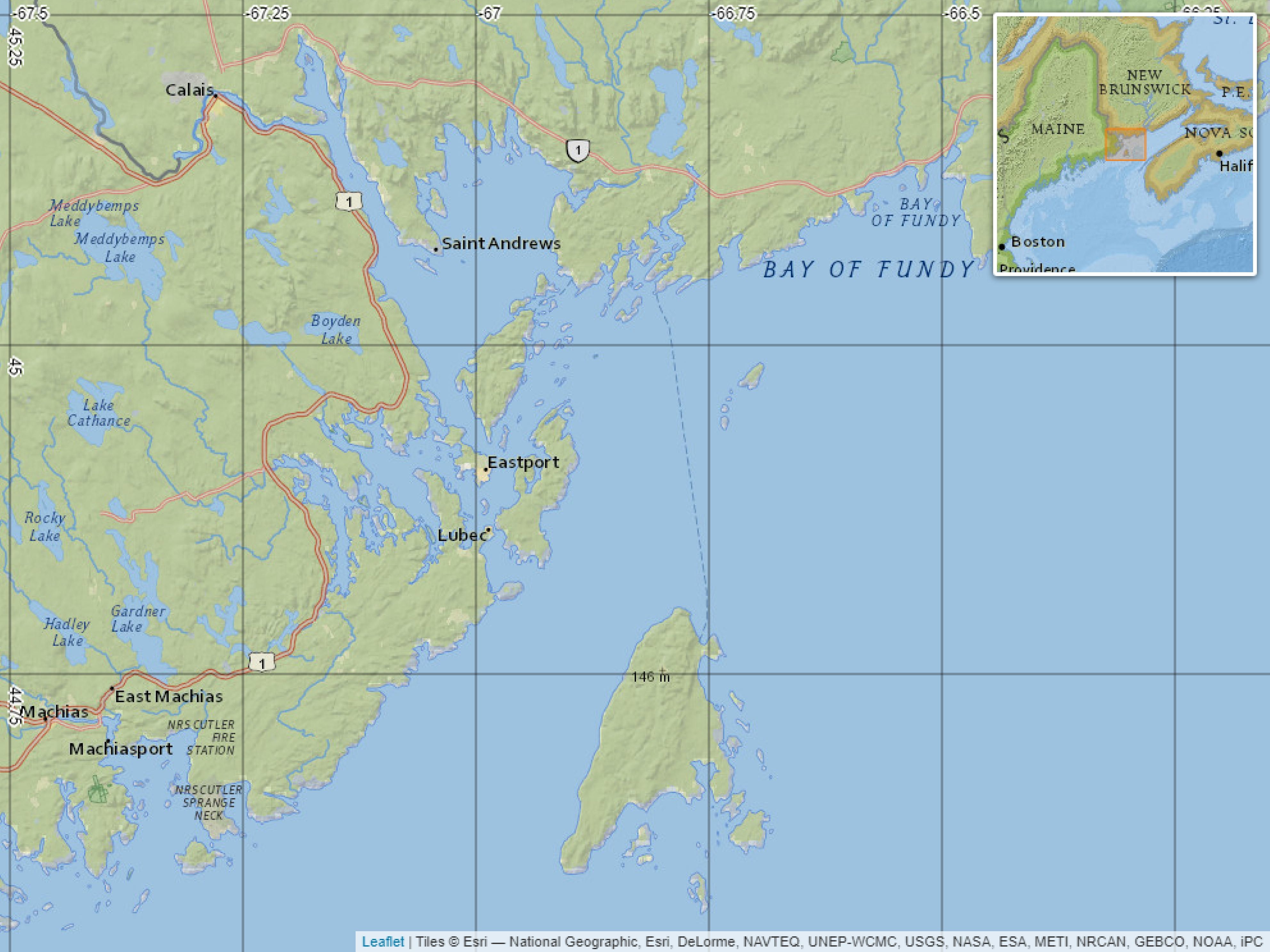
Figure 1. Area where salmon farms are located in New Brunswick (NB), Canada (57 farms). For detailed site locations, readers may consult the public Map Viewer of the Department of Aquaculture of the Government of New Brunswick (Marine Aquaculture Site Mapping Program, MASMP): https://www2.gnb.ca/content/gnb/en/departments/10/aquaculture/content/masmp.html.

2.2 Data and exploratory analysis

2.2.1 The Fish-iTrends database

The Fish-iTrends system, developed by the Atlantic Veterinary College-Centre for Aquatic Health Sciences (AVC-CAHS) at the University of Prince Edward Island in collaboration with the Atlantic Canada Fish Farmers Association (ACFFA), underpins the epidemiological model of sea lice dynamics in this study. The database contains abundance records of the parasitic sea lice, L. salmonis, including the life stages: chalimus (CHAL), adult female (AF), and pre-adult/adult male (PAAM). Although the system relies on submissions using multiple counters, which can contribute to counting and misclassification errors, the New Brunswick provincial government performs audits to compare site counters to independent official counters, and previous comparisons showed a general agreement with experienced counters, particularly for the adult female stages (Elmoslemany et al., 2013). It also includes geographic coordinates of the sampled farming sites, stocking and harvesting dates of farms, and sea lice treatment records. The treatment data include treatment start and end dates and treatment type (chemical, thermal, or mechanical delousing). Prior published research that used this database includes Parent et al. (2024b); Parent et al. (2021); Parent et al. (2024a); Elghafghuf et al. (2020), and Elghafghuf et al. (2021).

2.2.2 Data preparation and cleaning

The raw data obtained from the sea lice monitoring database underwent cleaning procedures to ensure accuracy and consistency. The main procedures, applied in the following order, included:

1. Outlier filtering: Obvious errors and extreme values in sea lice concentration were removed based on the 99.9th percentile thresholds.

2. Reconciliation of multiple weekly surveys: While weekly sampling was the norm (99.6% of 70,320 original records), some farming cycles had two surveys in the same week, often related to treatment events. To retain one record per week and farming cycle, a prioritization scheme was applied: post-treatment surveys were preferred, followed by regular weekly surveys, and then pretreatment surveys.

3. Imputation of missing observations: Missing weeks within a farming cycle were imputed using the most recent preceding observation (classified as free [F], low [L], high [H], or recovered [U]). For weeks immediately after stocking, infestation-free values and zero lice counts were assigned. The model was trained both with observed data only and with the inclusion of imputed values, and performance was evaluated under both scenarios.

4. Treatment data aggregation: Treatment information was aggregated from batch level (groups of fish treated simultaneously) to cage level to enable integration with sea lice monitoring data and facilitate analysis by farming cycle.

5. Outbreak identification: Sea lice outbreaks were defined as transitions to a high concentration of adult females (H) following a previous state of free (F), low (L), or recovered (U) within individual farming cycles. Consequently, for the purpose of analysis, if a widespread outbreak affects, for example, 20 neighboring farms, it is recorded as 20 distinct outbreak events, one per farm.

6. Exclusion of incomplete farming cycles: Farming cycles that lacked initial data, i.e., those that began before the first available observations, were excluded from further analysis.

2.2.3 Additional independent and derived variables

In addition to the variables reported within the Fish-iTrends database, a series of supplementary derived variables were calculated to ensure that the model considered as many possible pertinent factors to maximize applicability across diverse farming conditions. These derived variables include:

Average parasite load or concentration per fish: Computed by dividing the abundance of the different parasite life stages by the number of sampled fish, this variable indicates the average parasite load or concentration per individual fish by life stage of sea lice.

Farming cycle length: Farming cycles were identified using farm and cage identifiers, along with associated stocking and harvesting dates. To ensure temporal consistency, these dates were systematically reviewed. Among the 87,620 records in the original dataset, 17.7% contained stocking dates recorded as January 1st, and 5.4% had harvest dates as December 31st—likely reflecting default system values or placeholder entries in the absence of specific dates. These were changed to missing values for analysis. Chronological inconsistencies were also addressed: 0.4% of records listed stocking dates after the corresponding survey, and 2.9% listed harvest dates before it; in both cases, the date was adjusted to match the survey date to maintain internal coherence. The cleaned and corrected dates were then used to define farming cycles by site and cage.

Temporal information: The season, week of the year, and corresponding week of the initiation of the farming cycle were calculated for each sea lice survey record (after imputing missing values as explained later).

Distinct farm states: We classified the infestation status of fish into four categories based on the number of adult female (AF) sea lice per fish: free-of-adult-females (F), low concentration (L), high concentration (H), and fully recovered (U). The F state denotes the absence of AF since stocking, while U signifies that although no AF has been reported in the current week, infestation had taken place earlier in the production cycle. A threshold (above or equal) of 3 AF per fish was selected to differentiate low and high concentration levels. Adult females were selected as the focal life stage for modeling due to their relatively easier identification during monitoring (Gautam et al., 2016), which improves data reliability, and the key role of ovigerous females in parasite transmission. The chosen threshold is consistent with regulatory practices in regions such as Norway, Canada, and Chile (see review in the Introduction section).

Exposure to waterborne transmission of sea lice among farms: The cumulative exposure to waterborne transmission of AF (C_exp,AF) from surrounding (source) farms j (Equation 1) was calculated following Equations 1 and 2 by summing up the Gaussian kernel weights (G_ij) computed from the seaway distances (D_ij) to each active farm (AF_j) within a kernel’s bandwidth (σ) of 100 km to each (sink) farm i.

$\begin{array}{ll}{C}_{exp,AF}=\sum _j{G}_{ij}A{F}_j& (1)\end{array}$

$\begin{array}{ll}A{F}_j=\{\begin{array}{ll}0\hfill & \text{non}-\text{active\hspace{0.33em}farm}\hfill \\ 1\hfill & \text{active\hspace{0.33em}farm}\hfill \end{array}& (2)\end{array}$

The Gaussian kernel function, $G_{ij}$, is given by Equation 3:

$\begin{array}{ll}{G}_{ij}=\frac{1}{\sigma \sqrt{2\pi }}{e}^{-w_1}& (3)\end{array}$

The kernel incorporates a distance decay function ($w_1$), which allocates more weight to farms located closer than farms further away and was the distribution of choice for the transformation of seaway distance in multiple studies (e.g., Kristoffersen et al., 2013). The Gaussian weight (w₁) is given by Equation 4:

$\begin{array}{ll}{w}_1=e^{-\frac{D_{ij}^2}{2{\sigma }^2}}& (4)\end{array}$

According to Brewer-Dalton et al. (2014) and Wu et al. (2014), current speed in the Bay of Fundy varied from almost zero to over 100 cm s⁻¹, driven mainly by tidal forces. Brewer-Dalton et al. (2014) stated that sea lice dispersal stages last 1 to 10 days, with pre-infective stages traveling 10–100 km. Concordantly, a 100-km dispersal distance of sea lice was chosen, which coincides with the maximum observed seaway distances among farms in the study area. As a result, only farms within a seaway distance of 100 km were considered in the kernel density estimation. This distance allows the recognition of the potential influence of the more distant farms given the considerable water exchange in the study area, as well as the higher probability of significant influence from closer farms as evaluated in the study area by Parent et al. (2021) and Parent et al. (2024a).

Sea surface temperature (SST): SST was retrieved from the NOAA Multi-scale Ultra-high Resolution (MUR)-SST Analysis from 2009 to 2023. MUR-SST was preferred over in situ measurements from farm sites to avoid issues related to missing data and inconsistencies in measurement techniques. The MUR-SST is created using a combination of level-2 satellite observations and numerical models and provides daily global coverage with a spatial resolution of 1/25th of a degree (approximately 4 km). MUR-SST time series were used to train the model with realistic weekly variability. No comparison with other remote products was performed in this study.

Once the model was trained with MUR-SST data, a sinusoidal function was used to represent SST inputs in model simulations. This simplification replaced the full weekly time series with just two parameters: the mean SST and the annual amplitude, capturing seasonal variation while reducing input complexity in model simulations. This mathematical model is described by the equation:

$\begin{array}{ll}SST(t)=A·\sin (2\pi ft+\varphi )+C+noise& (5)\end{array}$

where SST(t) represents the seawater temperature at time t; A is the amplitude of the sinusoidal wave, governing the magnitude of the seasonal oscillations; f denotes the frequency of the sinusoidal wave, dictating the number of oscillations within a specified time period; ϕ signifies the phase shift of the sinusoidal wave, determining the horizontal displacement along the time axis; and C is the offset or mean value, indicating the annual mean sea surface temperature. Noise was added to the sinusoidal functions to simulate natural variation in SST(t), with the values drawn from a normal distribution centered at zero and having a standard deviation equal to the mean standard deviation of MUR-SST values averaged spatially for every week from 2009 to 2023.

For the initial fitting of the model to the observed data, the following initial parameter values were chosen: A = 1, f = 1/52 (assuming one cycle per year), phi = pi/4, and C was set to the mean temperature reported in the dataset. The optimization process utilized the Levenberg–Marquardt algorithm implemented through the nlsLM function in R (Elzhov et al., 2023). This algorithm aimed to minimize the difference between the modeled and observed temperatures, ensuring convergence for the non-linear least squares regression.

2.2.4 Odds ratio of sea lice prevalence

As part of the exploratory analysis, odds ratios were computed to assess the effectiveness of treatment in response to sea lice outbreaks. The odds ratio estimates the likelihood of recovery (either partial recovery from H to L or full recovery from H to U) in relation to a particular exposure (in this case, to sea lice treatment) relative to the likelihood of the outcome happening when that exposure is not present (no sea lice treatment). The statistical significance of observed variations in odds ratios was assessed using a chi-squared test that compares observed and expected values under the assumption of no link between exposure to treatments and infestation outcomes. The outcome prevalence, which refers to the proportion of the population that has the outcome of interest, i.e., recovery from H to L or H to U state, was also calculated from the 2 × 2 contingency table. Outcomes were observed up to 8 weeks after the outbreak was detected, as this was considered a reasonable timeframe to detect treatment responses to lice outbreaks. All calculations were derived using the “epi.2by2” function from the “epiR” package (Stevenson et al., 2013) within R (version 4.2.1). No distinction was made among treatment types (chemical, thermal, and mechanical delousing), and all were considered equally effective in the model.

2.3 Numerical model

2.3.1 Model development process

A discrete-time (week), first-order (it only depends on the state at the previous time t-1, not beyond that), multivariate Markov chain model was used to model categorical time series of AF sea lice infestation states at the scale of farming cycles based on Fish-iTrends data for New Brunswick farm sites. Model parameters were estimated using the Markov chain Monte Carlo (MCMC) methods to fit the model to data and obtain posterior distributions of parameters. The model includes four AF infestation states (boxes in Figure 2) and 12 possible weekly state transitions (arrows in Figure 2). Farms start in F (free of sea lice), may move to L (low infestation) or H (high infestation). From L or H, they can recover to U (full recovery), and from U, they can be reinfected (to L or H). L, H, and U represent the recurring states, as a return to the F state is not feasible. The probability equations governing state transitions are shown in section 4.4.1 and Supplementary Table S1 of the Supplementary Section.

Figure 2

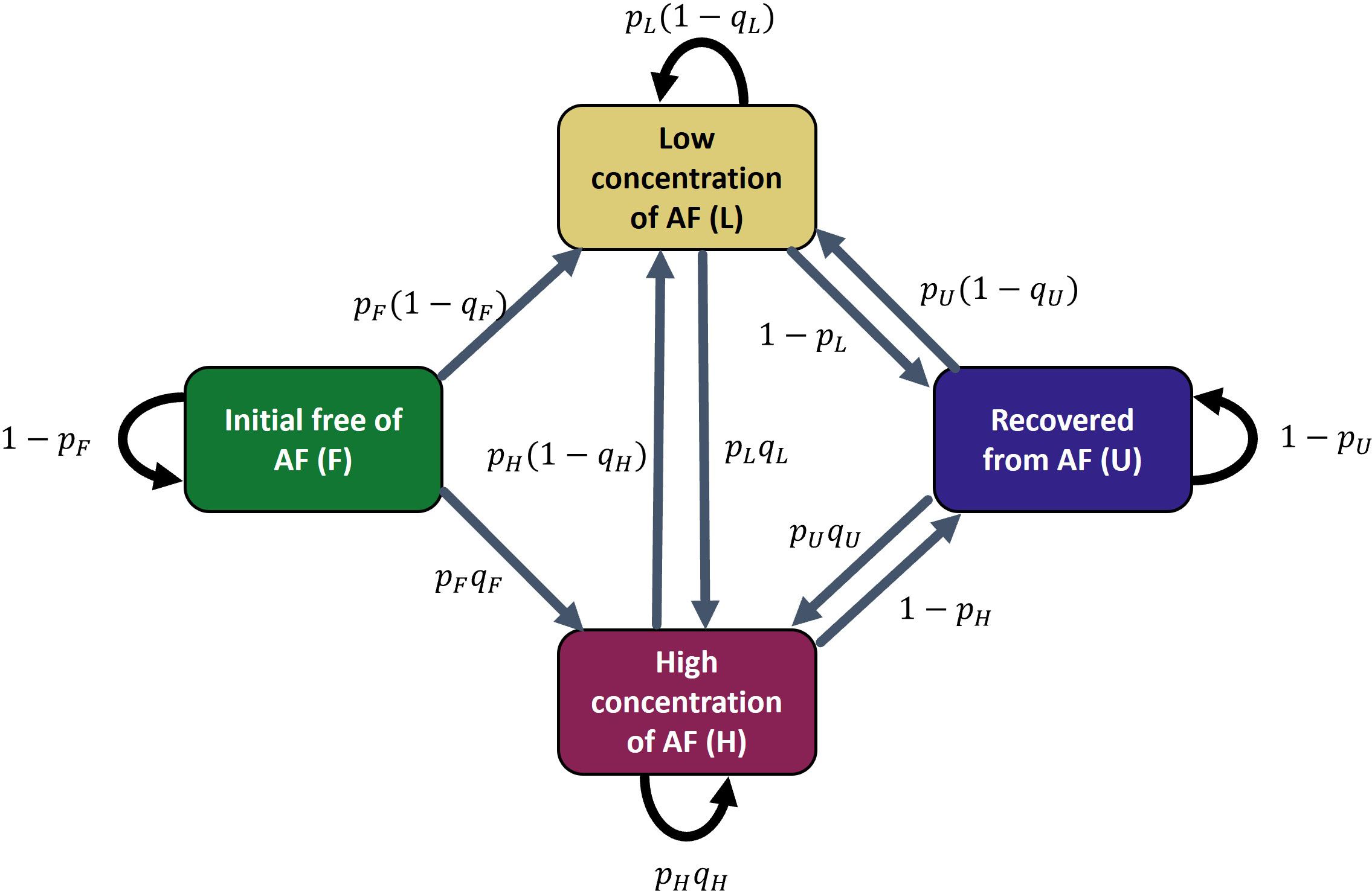
Figure 2. Markov chain model of infestation states. The model includes four infestation states (boxes) and 12 possible weekly state transitions (arrows). p_X = probability to move to an infestation state (L or H) given it is in the X state, and q_X = probability to move to the high infestation state given it is in the X state.

Transition probabilities were modeled as a function of the current infestation state and six time-dependent covariates: production cycle week, seaway distance-based exposure to neighboring farms, sea surface temperature, stocking week of the year, seasonal variation (modeled as a cosine function of week of the year), and treatment application (lagged by 1 week). Treatment effects, and related model parameters (aXv and bXv), were estimated conditional on infestation state (F, L, H, or U). This was required to account for potential confounding from infestation severity and was modeled as state-specific modifiers of infection probability (p) and severity (q), with aXv and bXv estimating the impact of treatment presence (see parameter definitions in the Supplementary Section). A penalization term was incorporated into the likelihood function to enforce biologically plausible constraints on treatment-related coefficients. Parameters controlling the effect of treatment on the infestation severity (bXv), specifically the transition to high infestation (H), were constrained to be negative (ensuring that treatment consistently reduces the probability of the H state).

Treatment effects and their corresponding model parameters (aXv and bXv, see Supplementary Tables S1 to 2 of the Supplementary Section) were estimated conditional on the infestation state (F, L, H, or U) to account for potential confounding by infestation probability and severity. A penalization term was added to the likelihood function to enforce biologically plausible constraints on treatment-related coefficients. In particular, parameters governing the effect of treatment on infestation severity (bXv), especially transitions to high infestation (H), were constrained to be negative, ensuring that treatment consistently reduces the likelihood of reaching the H state.

Effects were assumed to manifest 1 week after application, consistent with the model’s weekly temporal resolution. Model parameters were estimated by maximizing the likelihood of reproducing observed data, using a Markov chain approach to explore plausible stochastic transitions between observation times. Other potentially important covariates, such as fallow period, stocking density, stocking weight, and salmonid species, were not included due to a lack of available data during model development.

2.3.2 Assessment of model performance

The predictive performance of the stochastic, state-based model was evaluated by calculating the average probability of correctly predicting observed weekly transitions. The model was trained using the full dataset, and its predictive skill was assessed based on the total log-likelihood (LL) associated with the observed transitions. The average predictive probability was computed according to the following expression:

$$\exp (\frac{LL}{N})$$

where N denotes the total number of weekly transitions, with values closer to 1 corresponding to better performance.

To examine variation in model skill over time, the dataset was stratified into eight-time windows based on the number of weeks since stocking (i.e., 0–10, 10–20,…, 70–104 weeks). For each time window, the total log-likelihood and the number of transitions were computed, and the corresponding average predictive probability was estimated.

3 Results

3.1 Exploratory data analysis

3.1.1 Summary statistics

After data cleaning and preprocessing, the original dataset with more than 80k observations was reduced to 52,354 records, while the sea lice treatment dataset contained 25,868 observations (after aggregation from batch to cage level). Out of 57 farm sites (578 farm cages) in the sea lice monitoring database, 56 had treatment data (98.2%). A total of 1,365 fish farm cycles were recorded. By the end of the available survey records in December 2023, there were several farming cycles that were still ongoing. Ignoring these cases, the average length of the farming cycles was 99 weeks (1st quartile: 89 weeks; 3rd quartile: 109 weeks, max. 130 weeks). After imputation of missing values, the number of records doubled to 111,844.

Of the 111,844 records retained after data cleaning, preprocessing, and imputation, 59,490 (53.2%) were imputed—primarily as a low infestation (L, 25,401), followed by high infestation (H, 21,624). A smaller portion was imputed as free of adult females (F, 10,256), mostly at the beginning of the farming cycles (Figures 4A, B), and 2,209 as recovered (U). The remaining 52,354 records (46.8%) were original observations.

Stocking of cages was concentrated in spring and summer, while harvesting was distributed homogeneously throughout the year (Figures 3A, B, respectively). Sea lice treatments were concentrated in summer and fall, with few records during winter (Figure 3C). Sea lice treatments notably increased the weeks immediately after stocking, with a peak around week 10 of the farming cycle (Figure 3D).

Figure 3

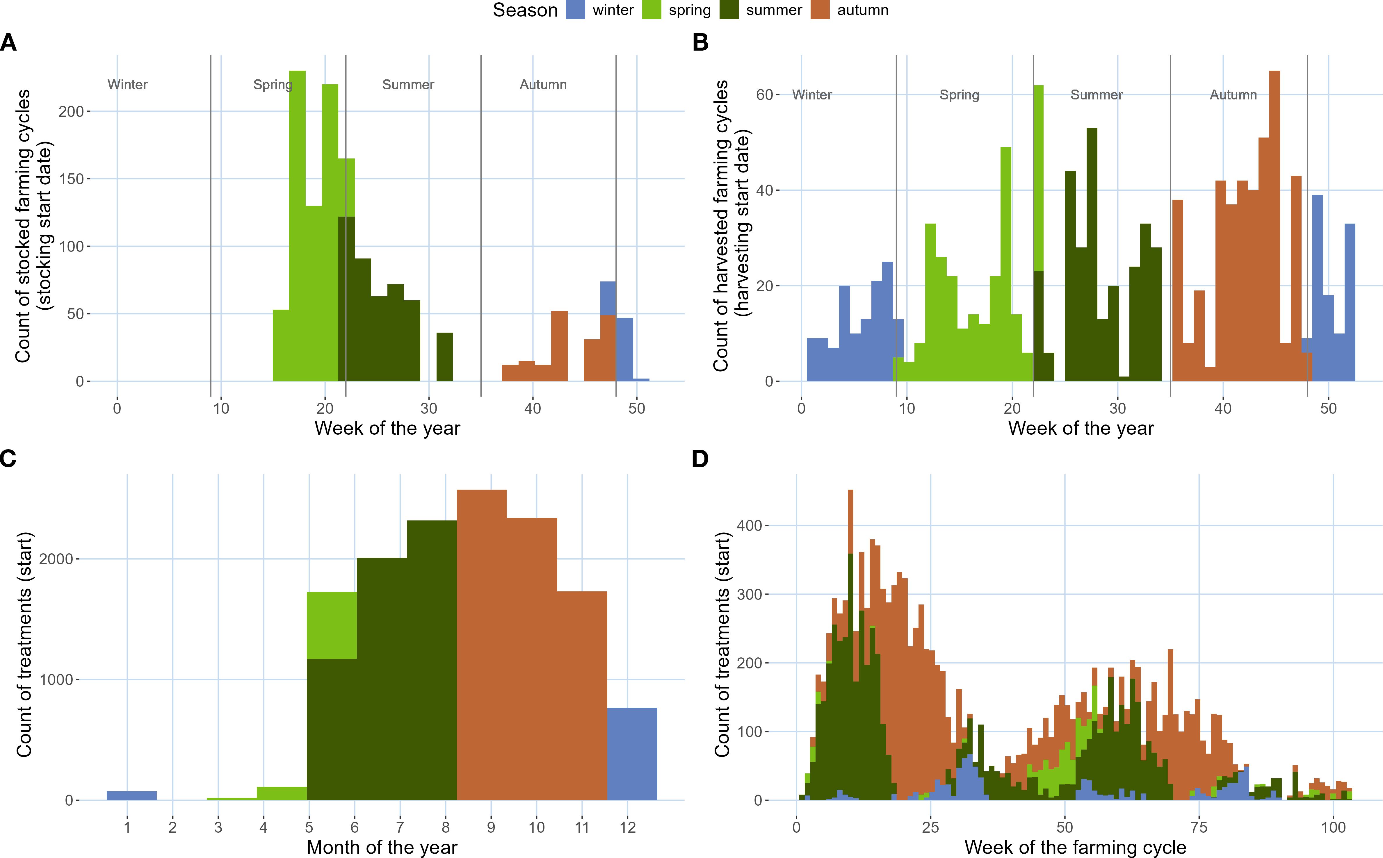
Figure 3. (A, B) Histograms of frequency of cage stocking (A) and cage harvesting (B) by week of the year and colored by season, based on Fish-iTrends data for New Brunswick farm sites (n = 57). (C, D) Histograms of the frequency of sea lice treatments by week of the farming cycle (C) and month of the year (D) and colored by season.

A high variability in the sea lice sampling efforts was evident in relation to both time of the year and week of the farming cycle. Sea lice surveys decayed both at the beginning and end of the farming cycles (Figure 4A), as well as in the wintertime (Figure 4B).

Figure 4

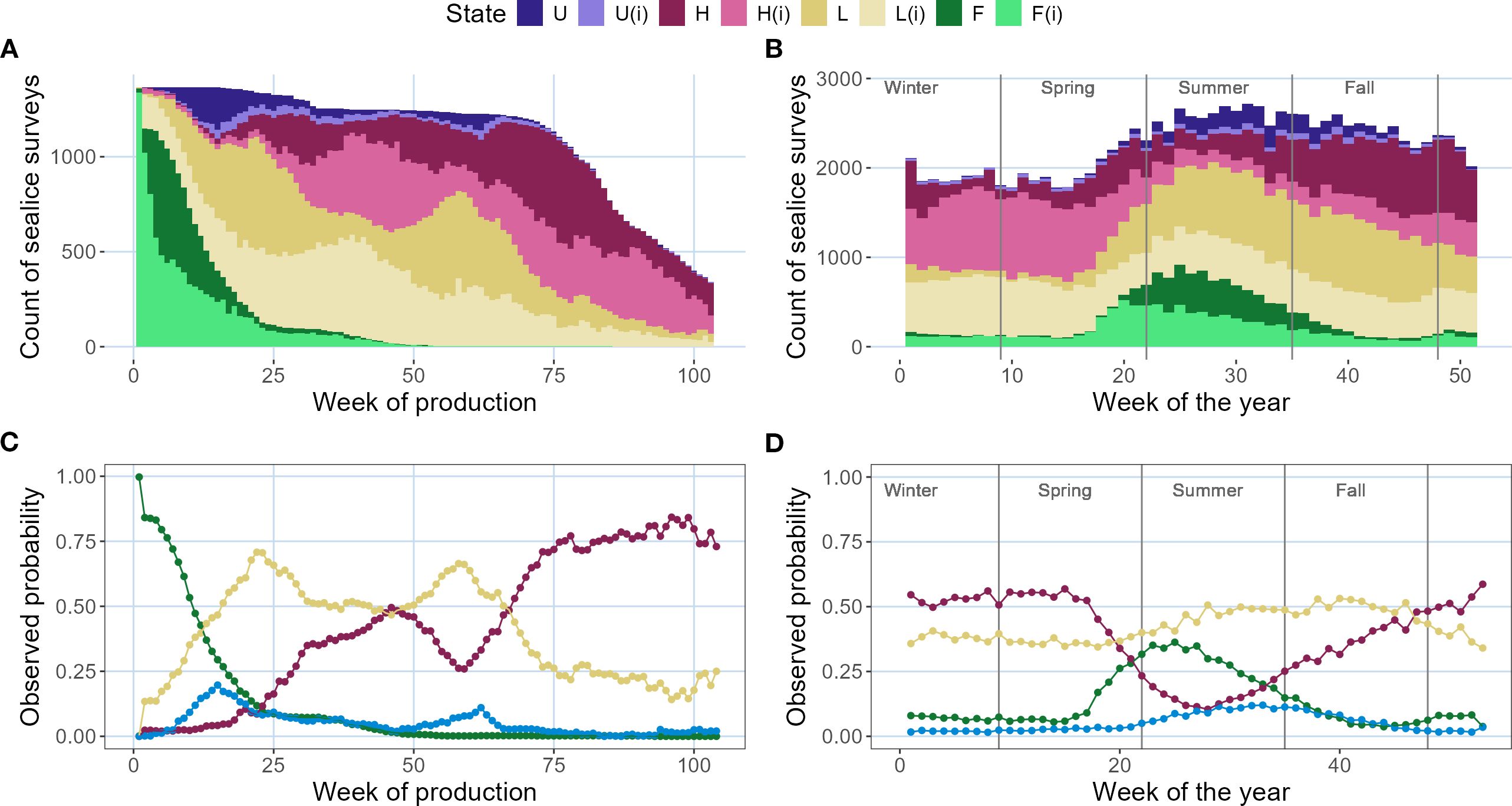
Figure 4. Histograms of sea lice survey counts by week of the farming cycle (A) and week of the year (B), including imputed (I) missing values shown in lighter colors, based on Fish-iTrends data for New Brunswick farm sites (n = 57). Observed probabilities (proportions) are displayed by week of the farming cycle (C) and week of the year (D). Colors indicate infestation states: F (free of adult females), H (high infestation), L (low), and U (recovered). The symbol i denotes imputed values.

3.1.2 Transition between the lice infestation states

The observed probabilities derived from empirical (frequency) data analysis are shown in Figures 4C, D. The observed probability of the initial free-of-adult-female (F) state, mostly observed in late spring and summer, remained above 75% until week ∼10 of the farming cycles. Nonetheless, after week ∼10, L became dominant in most of the fish farm cycles analyzed (Figure 4C). After week ∼60 of the farming cycle, the observed probability of H increased to over 50%, reaching values above 80% after week ∼75. Observed recovery (U) remained consistently low across all farming cycles and was nearly absent beyond week ∼75 of the farming cycle (Figure 4B). Some recovery was observed in summer and early fall (weeks ∼20 to ∼40 of the year), which coincided with the increased frequency of treatments in these seasons (Figure 3C). Equally noteworthy was the peak in the observed probability of high infestation (H) at week ∼45 of the farming cycle (red line, Figure 4C), which coincided with a decrease in treatments (Figure 3D). Treatments decrease especially in winter, as observed in Figure 3C.

As depicted in Figure S1 of the Supplementary Section, the probability of extremely high infestation events is much smaller compared to that of low concentration events, which are consistently observed within the dataset. That said, the objective of this modeling effort is not to predict extremely high infestation events but to focus on infestation levels that are known to endanger farmed fish, identified earlier as greater than or equal to 3 AF per fish.

3.1.3 Sea surface temperature

The mean sea surface temperature (MUR-SST) observed in the study area fluctuated annually between the coldest year in 2019 (7.90°C ± 4.03°C, observed range: 13.5°C, between 0.9°C and 14.4°C) and the warmest year in 2012 (9.61°C ± 3.89°C, observed range: 13.7°C, between 3.1°C and 16.8°C). The overall average temperature during this period was 8.60°C ± 3.89°C. Additionally, the range in year-round SST varied from 12.21°C in 2013 to 15.42°C in 2017 (Figure 5).

Figure 5

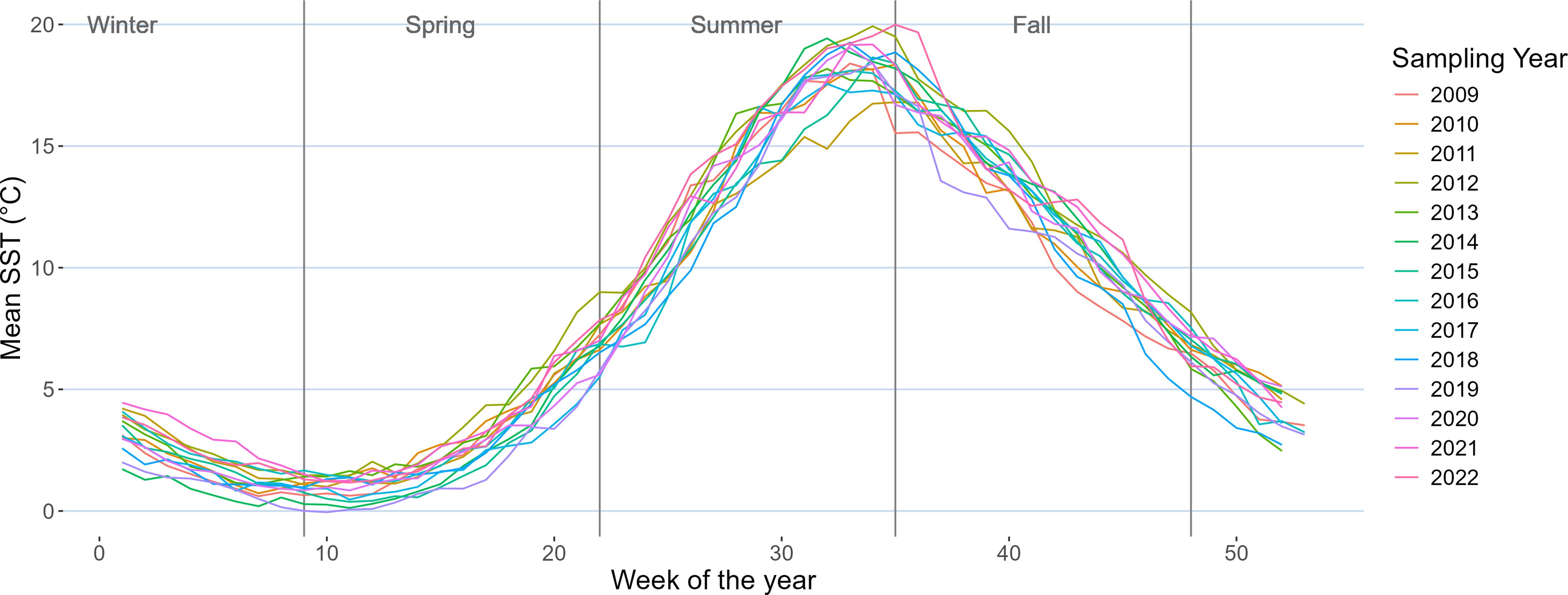
Figure 5. Time series of mean sea surface temperature (SST) from MUR-SST at 57 fish farm locations in the study area for the period 2009–2022.

3.1.4 Exposure to waterborne transmission of sea lice from surrounding farms

Exposure to waterborne transmission of sea lice from surrounding farms was estimated as a function of both the number of neighboring farms and their distance from each site. Farms with the highest potential exposure were primarily located in Passamaquoddy Bay, which showed elevated potential connectivity throughout the study area and time frame. On average, in NB, there were 41.2 fish farms within a 100-km radius, ranging from 11 to 56 farms.

3.1.5 Observed frequency of sea lice outbreaks and treatments

Between 2012 and 2023, a total of 8,596 sea lice outbreaks were recorded, defined as transitions to the high infestation state (H) from a preceding free (F), low (L), or recovered (U) state within individual farming cycles (see upper plot of Figure 6). Table 1 shows the differences in the proportions of sea lice outbreaks according to treatment exposure (treated or untreated) and the subsequent outcomes (recovery to state L or U) within 8 weeks after the outbreak was detected. The 2 × 2 contingency table presented in Table 1 shows that among the 8,596 sea lice outbreaks identified, 72.5% (n = 6,228) received treatment within the 8-week observation period, while the remaining 27.5% (n = 2,368) received no treatment during this period (but maybe after). Similarly, out of the total outbreaks, 76.0% (n = 6,531) transitioned from a high (H) state to either a low (L) or full recovery (U) within the same 8-week time frame, whereas 24.0% (n = 2,065) stayed in the high state throughout the entire 8-week observation period.

Figure 6

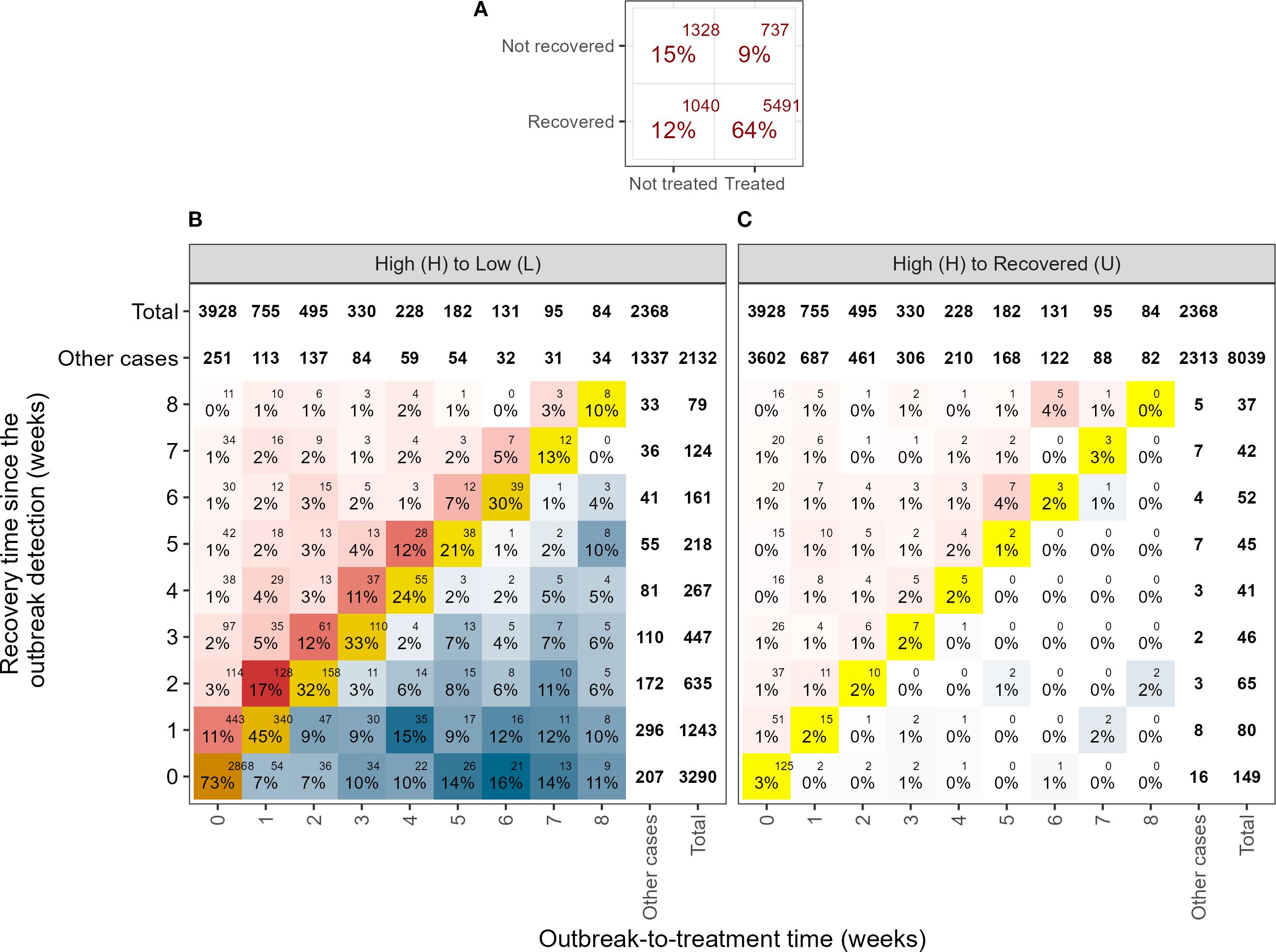
Figure 6. Number of detected outbreaks classified by recovery time, i.e. the total number of weeks it takes to transition from H to L state (panel B) or H to U state (panel C) and the outbreak-to-treatment duration, i.e. time elapsed since the outbreak detection to the administration of a sea lice treatment. The percentage values shown in each cell were computed relative to the total number of outbreaks with matching outbreak-to-treatment time (i.e. by column). No distinction was made between chemical, thermal or mechanical delousing. The “Other cases” category includes instances where recovery occurs after the observation period or corresponds to transitions shown in the complementary panel, i.e., recovery events of the other type (H to L or H to U), depending on the plot being viewed. Panel (A) shows a summary of treatment and recovery outcomes across all cases.

Table 1

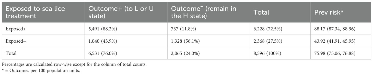
Table 1. Contingency table and summary measures of risk and a chi-squared test for differences in the observed proportions from count sea lice outbreaks by exposure to treatment and outcome (positive or negative).

Focusing on the 6,228 outbreaks that did receive treatment, 88.2% (n = 5,491) transitioned to either L or U states, while the remaining 11.8% (737 outbreaks) showed no change (Figure 6A). For the 2,368 untreated outbreaks, 43.9% (n = 1,040) transitioned to the L or U state within 8 weeks after the outbreak was detected, which is 44.3 percentage points lower than the treated group. The remaining 55.7% (1,328 outbreaks) did not recover within the 8-week observation period. Moreover, 75.2% (n = 4,683) of the outbreaks that were treated (n = 6,228) received a sea lice treatment within 2 weeks after recording an event of high concentration of AF.

The likelihood of recovery (from H to L or H to U) is 2.01 (with a confidence interval of 95% between 1.91 and 2.10) times higher in the outbreaks that received treatment (exposed group) compared to the outbreaks that did not receive treatment (unexposed group). A total of 89.5% of outcomes (either recovery or not) in the treated outbreaks were effectively attributed to sea lice treatments with a confidence interval of 95% between 88.9% to 90.2%), and the rest, 10.5%, were associated with other non-reported causes of recovery.

The database contains 6,677 records of sea lice concentrations measured the week before treatment. In 23.5% of the cases (1,567 records), the sea lice concentration was below the threshold of three lice per fish established in this study. In 73.4% (4,903 cases), the concentration was above that threshold before the treatment application. In only 3.1% of the cases, a sea lice concentration of zero was reported before sea lice treatment application.

The heat maps in Figure 6 display the number of detected outbreaks classified according to 1) the recovery time in the independent axis, which specifies the number of weeks elapsed from the outbreak (high infestation record) to the subsequent observation of either low (left panel) or complete recovery (right panel) independent of treatment administration, and 2) the outbreak-to-treatment time in the dependent axis, which specify the time elapsed since the outbreak detection to the administration of a sea lice treatment. The red and blue coloring of cells differentiates outbreaks where recovery was observed after (upper-left block of cells, red area) or before treatments (lower-right block of cells, blue area), respectively. Accordingly, the red-colored area represents recovery cases attributable to treatments or other causes, while the blue area indicates recovery not associated with the treatment. The diagonal cells, colored in yellow to orange, display the outbreaks in which treatment and recovery were reported the same week.

Transitions from high infestation to low infestation (Figure 6B) were notably more frequent than the transition from high infestation to full recovery (Figure 6C). In 54.4% (n = 4,762) of the outbreaks, the recovery to low or no infestation occurred within 2 weeks after detection of the outbreak, either due to treatment administration or other non-reported causes. In approximately 44% (n = 3,928) of the outbreak events, sea lice treatment was applied the same week of the outbreak, with a steady decline in the number of treatments applied in the weeks after, reaching a very small fraction by the eighth week.

When treatment was applied, the highest recovery was observed during the same week of application (as indicated by the diagonal cells in both panels of Figure 6). This immediate response is consistent with the rapid effect of mechanical or thermal delousing methods. In contrast, in-feed chemical treatments typically exhibit a delayed response, which may result in a more gradual decline in infestation levels over the weeks following treatment (Elghafghuf et al., 2020, 2018). However, this exploratory analysis and the model did not differentiate among treatment types, a limitation noted for future research.

The recovery rate seems to decrease as well when farms delay treatment in response to high infestations. For example, among the 3,928 outbreaks treated during the same week when a high concentration of AF lice was detected, 76% (n = 2,933) showed recovery from high (H) to low (L) or full recovery (U) within the same week, with an additional 12% (n = 502) recovering in the following week. In contrast, of the 755 outbreaks treated 1 week after detection, only 47% (n = 355) recovered during the week of treatment, and an additional 18% (n = 139) recovered the following week.

3.2 Model performance

As represented in Figure S3 in the Supplementary Section, the highest predictive accuracy was observed during the first 10 weeks post-stocking (74%), followed by a decrease and slight rebound later in the cycle. The overall average predictive accuracy across all transitions was 58.6% when considering only observed data and 57.5% when imputed data were included. Since data imputation did not improve model performance, only observed (non-imputed) records were used for model training and simulations.

3.3 Model simulations

3.3.1 Simulated time series

Figure 7 displays the simulated time series of multiple infestation states subject to different combinations of covariates and assuming treatment application the same week of detection of high infestation. Specifically, the simulation incorporates the exposure to waterborne transmission of sea lice among farms and the timing of fish farm stocking. Exposure to waterborne transmission of sea lice among farms was classified into four levels: low, medium–low, medium–high, and high, based on weekly quantiles (20th, 40th, 60th, and 80th percentiles) of the index of cumulative exposure to waterborne transmission of AF (C_exp,AF) calculated using Equation 1. This index was computed for each farm, year, and week of the year by summing the pairwise Gaussian distance weights between the focal farm and all neighboring farms classified as active (with fish on site) based on preidentified farming cycles. Weekly exposure values were then aggregated and averaged by farm site and week of the year to reflect temporal variability in infestation pressure. This method aims to capture both the spatial connectivity among farms and the variations of infestation risk due to fluctuating farm activity across time. Timing of fish farm stocking was input as week of the year, namely, mid-spring (week 15 of the year), mid-summer (week 28 of the year), and mid-fall (week 41 of the year). Stocking in mid-winter (approximately week 2 of the year) was not considered because they rarely happen based on the data available in this study. The simulation incorporated year-long time series of sea surface temperatures fitted to MUR-SST data (according to Equation 5) for a relatively cold (mean: 7.1°C, amplitude: 9.2°C), a warm (mean: 9.0°C, amplitude: 9.2°C), and an average condition (mean: 8.0°C, amplitude: 8.9°C).

Figure 7

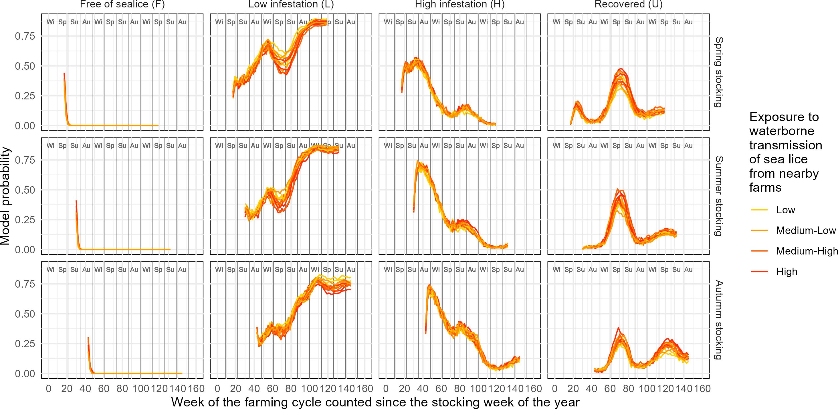
Figure 7. Simulated time series of multiple infestation states of AF subject to different combinations of covariates (stocking season, exposure to waterborne transmission of sea lice from surrounding farms and annual temperature regime.

Across all stocking seasons, farms initially remain in the F state only briefly, with rapid transitions to L or H occurring within the first 20 weeks. The timing and magnitude of these transitions vary with both stocking season and exposure level to sea lice transmission. For spring stocking, L states dominate much of the cycle, with H peaking between weeks 40 and 60, followed by a gradual rise in U, mediated by sea lice treatment. In summer stocking scenarios, H states rise earlier and more sharply, leading to earlier and more pronounced recovery (U). Autumn stocking delays the onset of infestation, but still results in a strong rise in H and U states around week 60. In all scenarios, higher exposure to sea lice from nearby farms consistently leads to elevated probabilities of H and U, underscoring the role of spatial transmission dynamics in infestation risk.

Exposure to waterborne transmission of sea lice influences both the speed and intensity of infestation buildup, although differences across scenarios are relatively modest. This may be due to the overall homogeneity in exposure levels across farms in the study area, with no cases of significantly isolated farms in the dataset. Under low or medium–low exposure, farms tend to remain in the F and L states for longer, with delayed or infrequent transitions to H and U. In contrast, under medium–high and high exposure, infestations escalate more rapidly, leading to earlier and more sustained occurrences of H and U states across all stocking seasons.

3.3.2 Integrated infestation probabilities across covariate scenarios

Figure 8 displays the integrated probabilities of the four infestation states, free (F), low (L), high (H), and fully recovered (U), over a 104-week salmon production cycle. These are not instantaneous or weekly probabilities of transitions or recovery but reflect the cumulative likelihood of each state across the entire farming cycle.

Figure 8

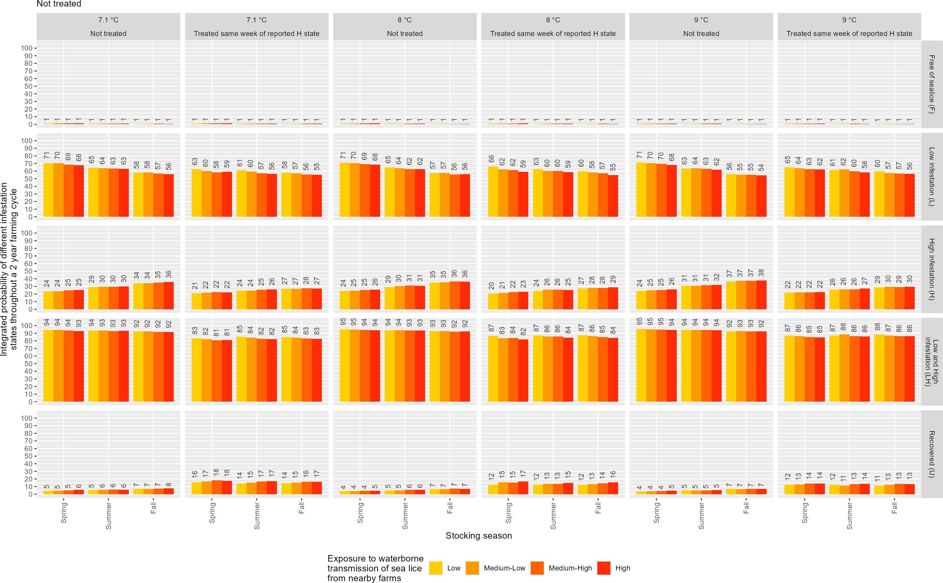
Figure 8. The integrated probability of various infestation states (F, L, H, and U) over a standard production cycle lasting 104 weeks (2 years), across multiple combinations of covariates: stocking season, exposure to waterborne transmission of sea lice, annual temperature regime, and sea surface temperature.

Simulations were conducted under varying conditions of treatment status (no treatment vs. treatment applied in the same week, high infestation was reported), mean sea surface temperature (7.1°C, 8.0°C, and 9.0°C), exposure to waterborne transmission (low, medium–low, medium–high, high), and stocking season (spring, summer, fall) as explained in the previous section.

The integrated probability of remaining free of adult female sea lice (F) was consistently low (<2%) across all scenarios. This indicates that even under favorable conditions, complete avoidance of infestation is unlikely in this study area, and this pattern showed minimal sensitivity to treatment, temperature, exposure level, or stocking season.

The probability of experiencing low infestation (L) over the full farming cycle varied across scenarios from ∼57% to ∼75%. In untreated cases, it ranged from approximately 61% (fall stocking, high exposure, 9.0°C) to 75% (spring stocking, low exposure, 7.1°C–9.0°C). With treatment, L increased modestly in most conditions, ranging from ∼57% to ∼73%. This suggests that timely treatment tends to reduce the likelihood of high infestation, while slightly increasing the probability of maintaining low infestation, particularly under warmer temperatures and higher exposure levels.

The probability of high infestation (H) was typically lower in treated scenarios. For instance, at 9.0°C and high exposure, fall stocking showed a decrease in H from 33% (untreated) to 28% (treated). The highest H probabilities were consistently associated with fall stocking and medium–high to high exposure levels, often exceeding 30% in untreated cases.

The combined probability of being in any infested state (L + H) surpassed 80% in nearly all spring and summer stocking scenarios, regardless of treatment. For example, at 8.0°C and medium–high exposure under spring stocking, the untreated groups showed a combined L + H probability of 95%.

Finally, the integrated probability of full recovery (U), defined as having zero observed adult female sea lice at any point during the production cycle, remained low overall across all scenarios. The probability of full recovery increased with sea lice treatment, especially under high exposure levels and in fall stocking scenarios, reaching up to 15%. In contrast, spring stocking consistently showed the lowest recovery probabilities, typically below 10%, regardless of treatment or exposure level. Summer stocking yielded intermediate results, with U ranging from ∼4% to 11%, depending on temperature and exposure.

4 Discussion

4.1 Key findings

4.1.1 Exploratory data insights

The exploratory analysis revealed that stocking events were predominantly concentrated in spring and summer, while harvesting activities were distributed more uniformly throughout the year. Farming cycles initiated in spring were significantly shorter than those starting in fall or summer, likely due to the accelerated growth rates associated with higher temperatures or earlier harvesting. For summer stocking, the earlier occurrence of high concentrations of AF lice may be attributable to elevated seawater temperatures, which are known to enhance lice development and survival (Johnson and Albright, 1991; Hamre et al., 2019), in combination with the increased number of active farms during this period, potentially elevating the risk of waterborne transmission of infective stages (Aldrin et al., 2013; Parent et al., 2021, 2024b) (see Figure S2 of the Supplementary Section). Future analyses could involve estimating degree-days to better explain variations in fish growth and the extent of farming cycles.

Elevated AF concentrations (≥3 lice per fish) were frequently found during winter months. This pattern is likely explained by the seasonal reduction in treatment activity due to logistical constraints imposed by weather (Westcott et al., 2004) and potentially by seasonal fluctuations in lice abundance (Fisheries and Oceans Canada, 2020; Rittenhouse et al., 2016). Seasonal cycles of sea lice abundance are well documented in Western Canada, where they are associated with wild salmon migrations that return to their spawning grounds in late summer (Fisheries and Oceans Canada, 2020). In Eastern Canada, in New Brunswick, fluctuations in sea lice abundance also correlate with changes in environmental conditions (Chang et al., 2011). Nearby, in Southern Newfoundland, the reproductive peak was found to be highly dependent on environmental conditions, particularly annual peaks in salinity levels (Rittenhouse et al., 2016).

Approximately 70% of outbreaks (i.e., transitions to the H state from a preceding F, L, or U state), received treatment within 2 months of detection. However, it is important to note that no mandatory treatment thresholds are established in the study area, and that due to data limitations, it was not possible to directly link treatment decisions to specific AF concentrations prior to treatments.

In most cases, the AF concentration at the time of treatment was at or above the 3 lice per fish threshold; however, in nearly one-quarter of the cases, treatments were administered when lice counts were below this threshold. This observation implies that sea lice treatments are not applied solely in response to high concentrations of AF, as defined in this study, but are determined most probably by a combination of logistic, economic, fish health factors, as well as treatment strategies within Bay Management Areas, that included product rotations and synchronized treatment (Atlantic Canada Fish Farmers Association (ACFFA), 2022).

Treatments were most often administered immediately following the detection of high AF concentrations (same week), with a sharp decline in treatment frequency thereafter. As a result, a greater proportion of outbreaks transitioned to low concentrations in the weeks immediately after detection. Treated outbreaks were notably more likely to transition to low or no infestation compared to untreated outbreaks, indicating the relative effectiveness of treatments. This is consistent with the findings from Gautam et al. (2017), who reported that post-treatment sea lice levels were lowest when counts were conducted 1 day after treatment, particularly in summer, suggesting a rapid and pronounced treatment response. However, they also observed that sea lice abundance increased again shortly after treatment during warmer months, indicating the short-lived nature of treatment effects and the potential for reinfestation. Consistent with this, the data available to this study show that approximately 33% of treatment events (by farming cycle, as defined in the Methods) were followed by a return to high infestation (H state) within 2 weeks, 39% within 3 weeks, and 43% within 4 weeks, indicating that nearly half of all post-treatment high infestations reoccurred relatively soon after intervention. Also interesting is the relatively high rate of recovery from high to low infestation observed in non-treated cases, which may be explained by natural declines or unreported contributing factors.

It is important to acknowledge the potential biases introduced by irregular sampling, as highlighted by Gautam et al. (2016) and Gautam et al. (2017). Infrequent sampling, particularly before and after treatment events, can affect estimates of infestation levels and treatment outcomes, thereby impacting epidemiological inferences. As a result, the findings presented here should be interpreted as approximations, with the understanding that unrecorded changes in infestation dynamics may have occurred between sampling points (e.g., sudden increases or declines in sea lice populations).

Finally, it is worth noting that extreme lice infestation events were infrequently represented in the training dataset (see Supplementary Figure 1). Although the modeling framework developed here was not specifically designed to predict such rare but impactful events, the integration of larger, multi-year datasets spanning additional farms in Atlantic Canada, along with complementary modeling approaches, may help improve predictive capacity for high-magnitude outbreaks in future research.

4.1.2 Model result insights

The complex dynamics arising from multiple covariates interacting simultaneously (seawater temperature, waterborne transmission, and stocking practices) were successfully reflected in changes in the weekly and integrated probabilities of various infestation states across a farming cycle.

Model infestation state transitions. High AF concentration, defined here as parasite loads equal to or exceeding 3 adult females per fish (AF), was influenced by high temperature, high exposure to waterborne transmission of sea lice from neighboring farms, stocking season (spring and summer), and sea lice treatment. These model patterns agreed with the studies in Norwegian marine salmon farms by Aldrin et al. (2013), where it was found that up to 28% of expected sea lice abundances were attributed to infection from neighboring farms, and the remaining cause was mostly attributed to infestation within farms. Infestation within farms was not assessed explicitly in this research, but implicitly because Markov chain models predict the future infestation state based on the current state. Alternatively, recovery was favored by sea lice treatments, particularly under decreased temperatures, as well as under reduced exposure to waterborne transmission of sea lice, and cage stocking during fall (and secondly late spring).

Effectiveness of sea lice treatments. The analysis of model outputs suggests that waterborne transmission of sea lice among farms may be reducing the effectiveness of treatments by facilitating persistent reinfection of treated populations. This effect is likely exacerbated by the high degree of spatial connectivity among farms in the study area. Exposure to waterborne transmission was estimated based on the number and proximity of neighboring farms, with no farms in the dataset classified as truly isolated. On average, farms in New Brunswick had 41.2 neighboring farms within a 100-km radius (ranging from 11 to 56). This limited variability in exposure restricts the model’s ability to explore treatment outcomes under more favorable conditions, such as those of spatially isolated farms with lower reinfection pressure. These findings underscore the importance of coordinated management within and beyond Bay Management Areas (BMAs) and highlight the need for advanced modeling tools that support robust scenario evaluation and improved decision-making (Guarracino et al., 2018; Stige et al., 2024).

4.2 Model assumptions and limitations

Recent global assessments have identified key limitations in modeling sea lice infection pressure, particularly related to transmission pathways, treatment efficacy, and environmental drivers, and introduced the concept of “knowledge strength” to emphasize the need for evaluating model reliability under uncertainty (Murphy et al., 2024; Moriarty et al., 2024; Murray et al., 2025). These insights highlight the importance of transparently stating model assumptions, several of which were required in this study and are outlined below to inform future research.

Homogeneous infestation-state of fish cohorts. It was assumed that all fish within a farm shared the same infestation state. While this simplification facilitates the formulation of the epidemiological model, it does not capture the internal infestation pressure, i.e., the potential transmission of sea lice within cage and between-cage. Furthermore, the internal infestation pressure (i.e., transmission within farms) is indirectly represented by conditioning a farm’s infestation state at each time step on its state in the previous week. Future model iterations should aim to incorporate finer-scale variability to more accurately reflect transmission dynamics.

Seaway distance as a proxy for waterborne transmission of sea lice among farms. In this Markov chain model, exposure to waterborne transmission from active neighboring farms is estimated using a kernel density approach based on seaway distances. Similarly, AF lice are used as a proxy for infestation pressure at source farms; nonetheless, it is their planktonic offspring, particularly the free-swimming copepodid stage, that are responsible for interfarm transmission. While seaway distance has been widely applied as a proxy for interfarm connectivity (Viljugrein et al., 2009; Stene et al., 2014; Bravo et al., 2020; Parent et al., 2024b) as it does not require the extensive computing processing power and time to run a hydrodynamic model, it may inadequately capture the biological and physical complexity of sea lice dispersal, which depends on larval behavior and hydrodynamic transport processes. To improve predictive performance, future efforts should prioritize the use of hydrodynamic (potential) connectivity rather than relying solely on seaway distance; however, these data are not available today in the study area. One step further, and in the context of real-time risk forecasting, model accuracy could be enhanced even more by incorporating realized connectivity, that is, hydrodynamic links filtered by the presence of active infestations at source farms capable of releasing eggs and motile larvae. Such refinements would provide a more realistic representation of transmission pathways and enable more accurate, targeted management interventions (Bravo et al., 2020; Asplin et al., 2020).

Seawater salinity. Seawater salinity was not available for this study at the farm level and for the entire period of analysis; therefore, it was not feasible to incorporate it into the model. Nonetheless, salinity levels are known to influence the viability of sea lice eggs (Brooker et al., 2018 and citations therein). Copepodids actively avoid salinity below 27 parts per thousand, expending energy for osmoregulation and maintaining position in seawater. Bricknell et al. (2006) have suggested that survival of free-swimming copepodids was found to be severely compromised at salinity levels below 29 parts per thousand (ppt), impairing their response to host cues. Planktonic stages are more susceptible to low salinity compared to parasitic stages that gain protection from close contact with the host and ingested host tissue (Brooker et al., 2018). Having access to salinity data from observation (in situ and remote) and modeling systems such as the Global Ocean Physics Analysis and Forecast system (available since November 2020 onward) could therefore meaningfully improve sea lice modeling.

Seawater temperature. The fluctuations in environmental conditions throughout the year significantly influence the dynamics of numerous disease systems as highlighted by Altizer et al. (2006), and more specifically for sea lice by Rittenhouse et al. (2016); Fast and Dalvin (2020), and Sandvik et al. (2021). In our study, MUR-SST time series were incorporated within the probabilistic model, allowing us to investigate its impact on probability of infestation and recovery. The probability of high concentration of AF increased for farms stocked in summer, coinciding with higher SST, while recovery was not particularly sensitive to SST. The integrated probabilities of infestation (combined L and H) does not change meaningfully with seasonal variations in SST between the coldest (mean: 7.90°C, amplitude: 13.5°C, derived from Equation 5) and warmest simulated condition (mean: 9.77°C, amplitude: 13.7°C, derived from Equation 5). Nonetheless, the effects of a warmer climate on salmon lice infection should not be disregarded as indicated by Sandvik et al. (2021). The correlation of SST with other factors such as fish biomass or host density per farm or farming area needs to be evaluated to differentiate between both effects. In this context, host density has been previously identified in the study area as a fundamental component of disease dynamics in coastal seas where salmon farming occurs (Frazer et al., 2012).

Fish growth. The lack of data on fish weight and/or size hindered the application of a growth model to the dataset. Such a model could have complemented the epidemiological framework by explicitly accounting for size-dependent differences in infestation risk and growth rates, including their dependence on temperature.

Other missing covariates. So far, we were able to incorporate as model covariates the exposure to waterborne transmission of sea lice from surrounding farms based on seaway distances, sea surface temperature from NASA PODAAC Multiscale Ultrahigh Resolution (MUR) Analyses, sea lice treatment, the stocking week of the year, and the week of the farming cycle. Although there was initial interest in including additional variables such as fish size at stocking, fish size at time of sea lice count, fish density (ind m⁻³, kg m⁻³, ton. cage⁻¹), relevant farming practices such as net cleaning, and seawater salinity, these factors could not be incorporated because the necessary data were not available for this study or were incomplete. Similar efforts of data integration for modeling have been done for other salmon diseases worldwide, demonstrating the potential benefits of such integration (Bravo et al., 2020; Aldrin et al., 2013; Ohlschuster et al., 2023; Steven et al., 2019). The imputation of missing values may have introduced bias into transition probability estimates, particularly for the “free” (F) state, the most frequently imputed category, specifically at the beginning of farming cycles. This could reduce the model’s sensitivity to environmental covariates and potentially mask early infestations that went undetected due to sparse monitoring.

Spatial gaps in data. Unfortunately, we were unable to include information from farms situated in the U.S. waters of Passamaquoddy Bay, as well as from other farms in the study region not owned by the collaborating company. The absence of these data could potentially compromise significantly the accuracy of our model, as it overlooks exposure to waterborne transmission of sea lice originating from those sites. Additionally, there may be other consequential impacts associated with the farming practices at these sites that are unknown and worth considering in future efforts of model development. The need to incorporate data at relevant spatial scales has also been highlighted in previous modeling studies within the study area (Elghafghuf et al., 2020, 2021). Furthermore, and related with sampling frequency, the data gap during the winter season and at the outset of production cycles may affect model training and performance. As a result, several decisions were made to impute missing values and to set the temporal resolution of the model (weekly).

Untangle the effects of seasonal environmental conditions from the effects of farming practices. SST varied throughout the year, but the number of active farms (which impacts the external infestation pressure) also varied seasonally, with most farms choosing to stock in spring, but harvesting more evenly across the year. In addition, environmental conditions and farming practices are not independent from each other, as certain environmental conditions can be an impediment (or an incentive) to certain practices or interventions, including sea lice surveys, treatment decisions, and stocking or harvesting (e.g., weather preventing sea lice counts and treatments during winter). Future work could try to ascertain if, for example, refining stocking schedules to promote staggered stocking dates of farms could help decrease external infestation pressure and support better fish health.

4.3 Implications for salmon farming in Eastern Canada

The sea lice model presented in this study has implications for the salmon farming industry in Eastern Canada. By offering a framework that integrates ecological insights and data-driven dynamics, the model may contribute to informed decision-making and the advancement of sustainable practices. Numerical models and applications, such as the one presented here, encapsulate institutional knowledge and experience accumulated over time. They offer advantages not just in aiding informed decision-making but also as a training tool for new employees or stakeholders within the aquaculture industry and regulatory agencies.

The model presented in this study, with further development, has the potential to support at least two types of farm decision-making in the future. The first are tactical decisions through short-term predictions of sea lice abundance and risk (days to weeks in advance) to support preventive measures, e.g., to protect the more vulnerable juvenile stages of salmon. To facilitate immediate decision-making, the model would require data transmission in real time, along with the processing (quality control) of captured data as it is acquired. The second benefit involves strategic decision-making pertaining to the stocking and harvesting of upcoming farming cycles and coordination beyond the farm’s limits, across BMAs or other management units. These decisions include anticipating the optimal stocking time, determining whether synchronized stocking impacts the overall performance of farms within the same management area or other spatial management units (e.g., a bay), assessing the significance of fallowing periods, and evaluating the effectiveness of treatments under varying environmental conditions and farming practices.

Data availability statement

The datasets analyzed in this study are part of the proprietary Fish-iTrend database and are not publicly available due to commercial confidentiality agreements. Access to these data may be requested directly from the data owner, subject to approval and data sharing conditions. Requests to access these datasets should be directed to KH, bGhhbW1lbGxAdXBlaS5jYQ==.

Ethics statement

This study involved the analysis of historical sea lice monitoring data collected from commercial salmon farms as part of routine health surveillance. No experimental procedures were performed on live animals for the purposes of this research. Therefore, ethical approval was not required in accordance with institutional and national guidelines.

Author contributions

FB: Writing – review & editing, Formal analysis, Writing – original draft, Visualization, Methodology, Validation, Data curation, Conceptualization, Software, Investigation. MO: Data curation, Investigation, Writing – review & editing, Software, Formal analysis, Methodology. MP: Data curation, Writing – review & editing, Methodology, Software, Investigation, Formal analysis. JK: Writing – review & editing, Investigation. TS: Writing – review & editing, Investigation. IG: Writing – review & editing. CW: Funding acquisition, Supervision, Project administration, Writing – review & editing, Investigation. RF: Investigation, Writing – review & editing, Funding acquisition, Supervision, Project administration. KH: Writing – review & editing, Validation, Data curation. AS: Writing – review & editing, Validation. LT: Investigation, Supervision, Project administration, Funding acquisition, Writing – review & editing. JG: Investigation, Writing – review & editing, Supervision, Funding acquisition, Project administration.

Funding

The author(s) declare financial support was received for the research and/or publication of this article. This work was supported by the Atlantic Fisheries Fund project “Big Data and Precision Fish Farming in Nova Scotia” (AFF-NS-1544).

Acknowledgments

We thank Matthew Sanford, programmer of the Fish-iTrends database, for his valuable insights.

Conflict of interest

AS is affiliated with Cooke Aquaculture Inc.

The remaining authors declare that the research was conducted in the absence of any commercial or financial relationships that could be construed as a potential conflict of interest.

Generative AI statement

The author(s) declare that Generative AI was used in the creation of this manuscript. Generative AI was used to support the preparation of this manuscript. It assisted with language editing, refine technical descriptions, and suggesting alternative phrasings during the revision process.

Any alternative text (alt text) provided alongside figures in this article has been generated by Frontiers with the support of artificial intelligence and reasonable efforts have been made to ensure accuracy, including review by the authors wherever possible. If you identify any issues, please contact us.

Publisher’s note

All claims expressed in this article are solely those of the authors and do not necessarily represent those of their affiliated organizations, or those of the publisher, the editors and the reviewers. Any product that may be evaluated in this article, or claim that may be made by its manufacturer, is not guaranteed or endorsed by the publisher.

Supplementary Material

The Supplementary Material for this article can be found onlineat: https://www.frontiersin.org/articles/10.3389/faquc.2025.1647026/full#supplementary-material

References

Abolofia J., Asche F., and Wilen J. E. (2017). The cost of lice: quantifying the impacts of parasitic sea lice on farmed salmon. Mar. Resource Econ 32, 329–349. doi: 10.1086/691981

Crossref Full Text | Google Scholar

Aldrin M., Storvik B., Kristoffersen A. B., and Jansen P. A. (2013). Space-time modelling of the spread of salmon lice between and within norwegian marine salmon farms. PloS One 8, e64039. doi: 10.1371/journal.pone.0064039

PubMed Abstract | Crossref Full Text | Google Scholar

Altizer S., Dobson A., Hosseini P., Hudson P., Pascual M., and Rohani P. (2006). Seasonality and the dynamics of infectious diseases. Ecol. Lett. 9, 467–484. doi: 10.1111/j.1461-0248.2005.00879.x

PubMed Abstract | Crossref Full Text | Google Scholar

Asplin L., Albretsen J., Johnsen I. A., and Sandvik A. D. (2020). The hydrodynamic foundation for salmon lice dispersion modeling along the norwegian coast. Ocean dynamics 70, 1151–1167. doi: 10.1007/s10236-020-01378-0

Crossref Full Text | Google Scholar

Atlantic Canada Fish Farmers Association (ACFFA) (2022). New Brunswick Annual Sea Lice Management Report 2022 (St. George, New Brunswick, Canada: Technical Report. Atlantic Canada Fish Farmers Association). Available online at: https://atlanticfishfarmers.com/wp-content/uploads/2024/06/ACFFA-2022-Sea-Lice-Mgt-Report.pdf.

Google Scholar

Bravo F., Sidhu J., Bernal P., Bustamante R., Condie S., Gorton B., et al. (2020). Hydrodynamic connectivity, water temperature, and salinity are major drivers of piscirickettsiosis prevalence and transmission among salmonid farms in Chile. Aquaculture Environ. Interact. 12, 263–279. doi: 10.3354/aei00368

Crossref Full Text | Google Scholar

Brewer-Dalton K., Page F. H., Chandler P., and Ratsimandresy A. (2014). may influence the biology and ecology of sea lice, lepeophtherius salmonis and caligus spp., and their control. DFO Can. Sci. Advis. Sec. Res. Doc. 2014/048. vi + 47 p. Available online at: https://publications.gc.ca/site/eng/9.801981/publication.html

Google Scholar

Bricknell I. R., Dalesman S. J., O’Shea B., Pert C. C., and Luntz A. J. M. (2006). Effect of environmental salinity on sea lice lepeophtheirus salmonis settlement success. Dis. Aquat. organisms 71, 201–212. doi: 10.3354/dao071201

PubMed Abstract | Crossref Full Text | Google Scholar

Brooker A., Skern-Mauritzen R., and Bron J. (2018). Production, mortality, and infectivity of planktonic larval sea lice, lepeophtheirus salmonis (krøyer 1837): current knowledge and implications for epidemiological modelling. ICES J. Mar. Sci. 75, 1214–1234. doi: 10.1093/icesjms/fsy015

Crossref Full Text | Google Scholar

Chang B. D., Page F. H., Beattie M. J., and Hill B. W. H. (2011). Sea louse abundance on farmed salmon in the southwestern new brunswick area of the bay of fundy. John Wiley Sons Ltd. chapter 3, 83–115. doi: 10.1002/9780470961568.ch3

Crossref Full Text | Google Scholar

Costello M. (2009). The global economic cost of sea lice to the salmonid farming industry. J. fish Dis. 32, 115. doi: 10.1111/j.1365-2761.2008.01011.x

PubMed Abstract | Crossref Full Text | Google Scholar

DMR (2025). Aquaculture map — department of marine resources. department of marine resources, state of maine, United States. Available online at: https://www.maine.gov/dmr/aquaculture/maine-aquaculture-leases-and-lpas/aquaculture-web-map (Accessed 2025-05-20).

Google Scholar

Elghafghuf A., Vanderstichel R., Hammell L., and Stryhn H. (2020). Estimating sea lice infestation pressure on salmon farms: Comparing different methods using multivariate state-space models. Epidemics 31, 100394. doi: 10.1016/j.epidem.2020.100394

PubMed Abstract | Crossref Full Text | Google Scholar

Elghafghuf A., Vanderstichel R., Hammell L., and Stryhn H. (2021). State-space modeling for intersite spread of sea lice with short-term population predictions. Ecol. Model. 452, 109602. doi: 10.1016/j.ecolmodel.2021.109602

Crossref Full Text | Google Scholar

Elghafghuf A., Vanderstichel R., St-Hilaire S., and Stryhn H. (2018). Using state-space models to predict the abundance of juvenile and adult sea lice on atlantic salmon. Epidemics 24, 76–87. doi: 10.1016/j.epidem.2018.04.002

PubMed Abstract | Crossref Full Text | Google Scholar

Elmoslemany A., Whyte S. K., Revie C. W., and Hammell K. L. (2013). Sea lice monitoring on a tlantic salmon farms in n ew b runswick, c anada: comparing audit and farm staff counts. J. Fish Dis. 36, 241–247. doi: 10.1111/jfd.12051

PubMed Abstract | Crossref Full Text | Google Scholar

Elzhov T. V., Mullen K. M., Spiess A. N., and Bolker B. (2023). minpack.lm: R Interface to the LevenbergMarquardt Nonlinear Least-Squares Algorithm Found in MINPACK, Plus Support for Bounds. Available online at: https://CRAN.R-project.org/package=minpack.lm.rpackage (Accessed January 15, 2024).

Google Scholar

Fast M. D. and Dalvin S. (2020). Lepeophtheirosis (lepeophtheirus salmonis)., in: Climate change and infectious fish diseases (Wallingford UK: CABI), 471–498. doi: 10.1079/9781789243277.0471

Crossref Full Text | Google Scholar

Fisheries and Oceans Canada (2020a). Sea lice management at bc salmon farms. Available online at: https://www.dfo-mpo.gc.ca/about-notre-sujet/publications/infographics-infographies/lice-pou-eng.html (Accessed May 22, 2025).

Google Scholar

Fisheries and Oceans Canada (2023b). Sea lice mitigation events graph. Available online at: https://www.pac.dfo-mpo.gc.ca/aquaculture/reporting-rapports/lice-mitigation-attenuation-poux/index-eng.html (Accessed May 22, 2025).

Google Scholar

Fisheries and Oceans Canada, 2023a Marine finfish aquaculture licence conditions – pacific region. Available online at: https://www.pac.dfo-mpo.gc.ca/aquaculture/licence-permis/docs/licence-cond-permis-mar/index-eng.html (Accessed May 22, 2025).

Google Scholar

Frazer L. N., Morton A., and Krkosek,ˇ M. (2012). Critical thresholds in sea lice epidemics: evidence, sensitivity and subcritical estimation. Proc. R. Soc. B: Biol. Sci. 279, 1950–1958. doi: 10.1098/rspb.2011.2210

PubMed Abstract | Crossref Full Text | Google Scholar

Gautam R., Boerlage A., Vanderstichel R., Revie C., and Hammell K. (2016). Variation in pre-treatment count lead time and its effect on baseline estimates of cage-level sea lice abundance. J. fish Dis. 39, 1297–1303. doi: 10.1111/jfd.12460

PubMed Abstract | Crossref Full Text | Google Scholar

Gautam R., Vanderstichel R., Boerlage A., Revie C., and Hammell K. (2017). Effect of timing of count events on estimates of sea lice abundance and interpretation of effectiveness following bath treatments. J. Fish Dis. 40, 367–375. doi: 10.1111/jfd.12519

PubMed Abstract | Crossref Full Text | Google Scholar

Government of Canada, S.C (2023). Table 32-10-0107–01 aquaculture, production and value. Available online at: https://www150.statcan.gc.ca/t1/tbl1/en/tv.action?pid=3210010701&pickMembers%5B0%5D=1.5&pickMembers%5B1%5D=2.3&cubeTimeFrame.startYear=2018&cubeTimeFrame.endYear=2022&referencePeriods=20180101%2C20220101 (Accessed May 13, 2025).

Google Scholar

Guarracino M., Qviller L., and Lillehaug A. (2018). Evaluation of aquaculture management zones as a control measure for salmon lice in Norway. Dis. Aquat. organisms 130, 1–9. doi: 10.3354/dao03254

PubMed Abstract | Crossref Full Text | Google Scholar

Guttu M., Gaasø M., Batnes A. S., and Olsen Y. (2024). The decline in sea lice numbers during freshwater treatments in salmon aquaculture. Aquaculture 579, 740131. doi: 10.1016/j.aquaculture.2023.740131

Crossref Full Text | Google Scholar

Hamre L. A., Bui S., Oppedal F., Skern-Mauritzen R., and Dalvin S. (2019). Development of the salmon louse lepeophtheirus salmonis parasitic stages in temperatures ranging from 3 to 24 c. Aquaculture Environ. Interact. 11, 429–443. doi: 10.3354/aei00320

Crossref Full Text | Google Scholar

Hamre L. A., Eichner C., Caipang C. M. A., Dalvin S. T., Bron J. E., Nilsen F., et al. (2013). The salmon louse lepeophtheirus salmonis (copepoda: Caligidae) life cycle has only two chalimus stages. PloS One 8, 1–9. doi: 10.1371/journal.pone.0073539

PubMed Abstract | Crossref Full Text | Google Scholar

Jevne L. S. (2020). Development and Dispersal of Salmon Lice (Lepeophtheirus salmonis Krøyer 1837) in Commercial Salmon Farming Localities. Norwegian University of Science and Technology (NTNU, Trondheim, Norway. Available online at: https://ntnuopen.ntnu.no/ntnu-xmlui/handle/11250/2670045. Phd thesis (Accessed May 22, 2025).

Google Scholar

Johnson S. and Albright L. (1991). Development, growth, and survival of lepeophtheirus salmonis (copepoda: Caligidae) under laboratory conditions. J. Mar. Biol. Assoc. United Kingdom 71, 425–436. doi: 10.1017/S0025315400051687

Crossref Full Text | Google Scholar

Kristoffersen A., Rees E., Stryhn H., Ibarra R., Campisto J. L., Revie C., et al. (2013). Understanding sources of sea lice for salmon farms in Chile. Prev. veterinary Med. 111, 165–175. doi: 10.1016/j.prevetmed.2013.03.015

PubMed Abstract | Crossref Full Text | Google Scholar

Ministry of Fisheries and Coastal Affairs (Norway) Regulation No. 1140 on control of salmon lice in aquaculture. Available online at: https://www.fao.org/faolex/results/details/en/c/LEX-FAOC118502/ (Accessed May 22, 2025).

Google Scholar

Moriarty M., Murphy J. M., Brooker A. J., Waites W., Revie C. W., Adams T. P., et al. (2024). A gap analysis on modelling of sea lice infection pressure from salmonid farms. i. a structured knowledge review. Aquaculture Environ. Interact. 16, 1–25. doi: 10.3354/aei00469

Crossref Full Text | Google Scholar

Mowi A. S. A. (2025). Integrated pest management (ipm) for sea lice control policy. Available online at: https://mowi.com/wp-content/uploads/2025/04/Mowi-Policy-on-Integrated-Pest-Management.pdf (Accessed 2025-05-22).

Google Scholar

Murphy J. M., Moriarty M., Brooker A. J., Waites W., Revie C. W., Adams T. P., et al. (2024). A gap analysis on modelling of sea lice infection pressure from salmonid farms. ii. identifying and ranking knowledge gaps: output of an international workshop. Aquaculture Environ. Interact. 16, 27–42. doi: 10.3354/aei00471

Crossref Full Text | Google Scholar

Murray A., Asplin L., a Nordi G., Erenbjerg S., Gallego A., Ives S. C., et al. (2025). knowledge strength”: maximising the reliability of evidence derived from environmental modelling in the face of uncertainty–the case of the salmon louse (lepeophtheirus salmonis). Socio-Environmental Syst. Model. 7, 18750–18750. doi: 10.18174/sesmo.18750

Crossref Full Text | Google Scholar

Ohlschuster M., Comiskey D., Kavanagh M., Kickinger F., Scaldaferri C., Sigler M., et al. (2023). On the prediction of sav transmission among norwegian aquaculture sites. Prev. Veterinary Med. 224, 106095. doi: 10.1016/j.prevetmed.2023.106095

PubMed Abstract | Crossref Full Text | Google Scholar

Parent M. I., Stryhn H., Hammell K. L., Fast M. D., Fast M. D., and Vanderstichel R. (2024a). Predicting the abundance of lepeophtheirus salmonis in the bay of fundy, new brunswick. J. Aquat. Anim. Health 36 (4), 355–373. doi: 10.1002/aah.10235

PubMed Abstract | Crossref Full Text | Google Scholar

Parent M. I., Stryhn H., Hammell K. L., Fast M. D., Grant J., and Vanderstichel R. (2021). Estimating the dispersal of lepeophtheirus salmonis sea lice within and among atlantic salmon sites of the bay of fundy, new brunswick. J. Fish Dis. 44, 1971–1984. doi: 10.1111/jfd.13511

PubMed Abstract | Crossref Full Text | Google Scholar

Parent M. I., Stryhn H., Hammell K. L., Grant J., and Vanderstichel R. (2024b). Estimation and comparison of connectivity measures for the dispersal of lepeophtheirus salmonis sea lice among atlantic salmon farms in new brunswick, Canada. J. Exp. Mar. Biol. Ecol. 572, 151992. doi: 10.1016/j.jembe.2024.151992

Crossref Full Text | Google Scholar

Rittenhouse M. A., Revie C. W., and Hurford A. (2016). A model for sea lice (lepeophtheirus salmonis) dynamics in a seasonally changing environment. Epidemics 16, 8–16. doi: 10.1016/j.epidem.2016.03.003

PubMed Abstract | Crossref Full Text | Google Scholar

Sandvik A. D., Dalvin S., Skern-Mauritzen R., and Skogen M. D. (2021). The effect of a warmer climate on the salmon lice infection pressure from norwegian aquaculture. ICES J. Mar. Sci. 78, 1849–1859. doi: 10.1093/icesjms/fsab069

Crossref Full Text | Google Scholar

SERNAPESCA (2014). Informe tecnico:´Nueva estrategia de programa de control de caligidosis. Valparaiso, Chile: National Fisheries and Aquaculture Service (SERNAPESCA).

Google Scholar

SERNAPESCA (2022). Res. ex. n° 60 - 02.02.2022 — aprueba programa sanitario espec´ıfico de vigilancia y control de la caligidosis (psevc-caligidosis). Valparaiso, Chile: National Fisheries and Aquaculture Service (SERNAPESCA).

Google Scholar

Stene A., Viljugrein H., Yndestad H., Tavornpanich S., and Skjerve E. (2014). Transmission dynamics of pancreas disease (pd) in a norwegian fjord: aspects of water transport, contact networks and infection pressure among salmon farms. J. fish Dis. 37, 123–134. doi: 10.1111/jfd.12090

PubMed Abstract | Crossref Full Text | Google Scholar

Steven A. D., Aryal S., Bernal P., Bravo F., Bustamante R. H., Condie S., et al. (2019). Sima austral: An operational information system for managing the Chilean aquaculture industry with international application. J. Operational Oceanography 12, S29–S46. doi: 10.1080/1755876X.2019.1636606

Crossref Full Text | Google Scholar

Stevenson M., Nunes T., Sanchez J., Thornton R., Reiczigel J., Robison-Cox J., et al. (2013). epir: An r package for the analysis of epidemiological data. r package version 0.9-48 (Vienna, Austria: R Foundation for Statistical Computing).

Google Scholar

Stien A., Bjørn P. A., Heuch P. A., and Elston D. A. (2005). Population dynamics of salmon lice lepeophtheirus salmonis on atlantic salmon and sea trout. Mar. Ecol. Prog. Ser. 290, 263–275. doi: 10.3354/meps290263

Crossref Full Text | Google Scholar

Stige L. C., Jansen P. A., and Helgesen K. O. (2024). Effects of regional coordination of salmon louse control in reducing negative impacts of salmonid aquaculture on wild salmonids. Int. J. Parasitol. 54 (8–9), 463–474. doi: 10.1016/j.ijpara.2024.04.003

PubMed Abstract | Crossref Full Text | Google Scholar

Viljugrein H., Staalstrøm A., Molvær J., Urke H., and Jansen P. (2009). Integration of hydrodynamics into a statistical model on the spread of pancreas disease (pd) in salmon farming. Dis. Aquat. organisms 88, 35–44. doi: 10.3354/dao02151

PubMed Abstract | Crossref Full Text | Google Scholar

Westcott J. D., Hammell K. L., and Burka J. F. (2004). Sea lice treatments, management practices and sea lice sampling methods on atlantic salmon farms in the bay of fundy, new brunswick, Canada. Aquaculture Res. 35, 784–792. doi: 10.1111/j.1365-2109.2004.01101.x

Crossref Full Text | Google Scholar

Wu Y., Chaffey J., Law B., Greenberg D. A., Drozdowski A., Page F., et al. (2014). A threedimensional hydrodynamic model for aquaculture: a case study in the bay of fundy. Aquaculture Environ. Interact. 5, 235–248. doi: 10.3354/aei00108

Crossref Full Text | Google Scholar