A Suite of Tools for Continuous Land Change Monitoring in Google Earth Engine

Introduction

Remote sensing of the land surface can contribute to our understanding of the climate system in a variety of ways. The land surface represents the boundary conditions for atmospheric circulation models, providing essential information on exchanges of mass, energy and momentum between the surface and the atmosphere (Sellers et al., 1997). The Global Climate Observing System (GCOS) has identified Essential Climate Variables (ECVs), which include a suite of land surface products related to the cryosphere, biosphere, and hydrosphere that are “needed to understand and predict the evolution of climate, to guide mitigation and adaptation measures, to assess risks and enable attribution of climate events to underlying causes, and to underpin climate services” (WMO, 2020). In this paper, we focus on one of these Climate ECVs, land cover, with particular attention to change in land cover as it has been a primary driver of increases in atmospheric CO₂. Historically, more than half of the CO₂ added to the atmosphere by humans can be attributed to land use and land cover change, which releases large amounts of carbon, often from burning of biomass (Houghton and Nassikas, 2017). Land use and land cover change remain as important sources of greenhouse gases, and for this reason the REDD+ program was created. By the time the REDD+ program started, ~12% of the annual carbon emissions were due to land use practices, including deforestation and forest degradation (Houghton et al., 2012; Goetz et al., 2015). The REDD+ Program, an abbreviation of Reducing emissions from deforestation and forest degradation and the role of conservation, sustainable management of forests and enhancement of forest carbon stocks in developing countries, was designed to reduce greenhouse gas emissions from the land sector by providing economic incentives. The program stipulates that developing countries will receive economic compensation for measuring, verifying, and reporting on reductions of greenhouse gas emissions from one or more of the five REDD+ activities: (1) deforestation, (2) forest degradation; (3) conservation, (4) sustainable management, and (5) enhancement of forest carbon stocks (GFOI, 2016). Thus, land cover change monitoring and reporting by participating countries is at the heart of the REDD+ Program.

Monitoring land surface change has been one of the primary uses of remote sensing over the past several decades. The most common approach has been to compare images from before and after the changes of interest to map the location, extent and kinds of change. This approach can be thought of as using satellite images as “endpoints” to monitor change. There are many examples in the literature, most of which have used data from the Landsat Program (Coppin and Bauer, 1996; Hansen and Loveland, 2012; Zhu, 2017). The Landsat Program has been collecting global data since 1972, and since 1982 a series of four satellites have collected data at 30 m spatial resolution, providing an archive of imagery valuable for monitoring land change over decades. Many other sensors have also been used for monitoring land change. The MODIS sensors on Terra and Aqua have been frequently used for monitoring change, particularly fires (Giglio et al., 2018). However, the relatively coarse spatial resolution of MODIS (250 m for the NIR and red bands and 500 m for the other “land bands”) has limited its utility for monitoring land use change, which often occurs over much smaller areas. More recently, the Copernicus Program has launched the Sentinel-1 (2014 and 2016) and Sentinel-2 (2016) series of satellites, which have begun collecting data suitable for monitoring land change. Sentinel-1 is a C-Band Synthetic Aperture Radar that has four operating modes, which collect data at spatial resolutions that range from 5 to 25 m. The Sentinel-2 satellites collect visible and near infrared data at 10 m spatial resolution and shortwave infrared and several specialized bands (e.g., red edge) at 20 m. There are also spectral bands at 60 m spatial resolution, that are primarily used for atmospheric characterization.

Since the advent of free data from the Landsat Program in 2008, new methodologies for mapping land cover change based on analysis of many observations (or time series) have emerged. Rather than rely on a pair of observations before and after to detect a change, algorithms can now be used to monitor land change in a more continuous fashion (Woodcock et al., 2020). The first time-series approaches used a single observation for each year, enabling the detection of changes on an annual basis (Huang et al., 2010; Kennedy et al., 2010; Hughes et al., 2017). These algorithms were usually based on a single spectral index and were designed to find specific types of change, often change in forests. Other methods that used MODIS data (usually NDVI, the Normalized Difference Vegetation Index) composited to 16 or 32 day time periods to look for land change were developed simultaneously (Verbesselt et al., 2010). Over time, more emphasis has been placed at Landsat resolutions on using more than annual observations to better understand the timing and dynamics of land change. One approach that attempts to use all good quality observations is CCDC [Continuous Change Detection and Classification (Zhu and Woodcock, 2014)], which is intended to be a general-purpose algorithm for finding many kinds of changes in a continuous manner and mapping the land cover before and after. Parallel efforts have attempted to study and characterize land surface phenology using the information contained in time series of remote sensing observations directly, rather than deriving land cover data from them. Some examples include the study of trends in spring onset and fall phenology (Schwartz et al., 2006; Dragoni and Rahman, 2012), crop yield forecasting (Bolton and Friedl, 2013), global phenology products and intercomparisons (Ganguly et al., 2010; Moon et al., 2019), among other applications (Morisette et al., 2009; Henebry and Beurs, 2013). Land surface phenology is an important but extensive research topic that is beyond the scope of this paper. For this reason, we will focus exclusively on land cover and land cover change mapping.

The relationship between REDD+ and Landsat is essential because Landsat is frequently the most viable data option for REDD+. For example, countries are required to establish a Forest Reference Level (FREL) against which more recent emissions can be compared, often requiring multiple decades of images to contribute to the establishment of FRELs and monitoring thereafter. For many of those countries, using Landsat data is the most plausible option due to its relatively high resolution, availability since the 1980's for many regions in the world, and consistent pre-processing and archival in collections that allow the delivery of high-quality surface reflectance products (Olander et al., 2008; USGS, 2018). Additionally, the Landsat Program has improved the processing and consistency of their datasets by including atmospheric correction, cloud and cloud shadow masking and improved multitemporal registration, while providing the data at no cost to the user (Zhu and Woodcock, 2014; Vermote et al., 2016). Furthermore, the development of algorithms to harmonize Landsat and Sentinel-2 surface reflectance products is expected to augment these collections with data of similar characteristics (Claverie et al., 2018). However, providing the necessary satellite data is just the first step – subsequent steps include determining the best use for the data to monitor REDD+ activities in ways compliant with the Intergovernmental Panel on Climate Change criteria and also useful for decision- and policy-making.

To achieve compliance, effective and comprehensive monitoring in countries where it is needed the most, capacity building efforts have been sponsored and organized by various organizations including SilvaCarbon, USAID, UN-FAO, NASA-SERVIR, and GOFC-GOLD. As direct and active participants in these efforts, we have witnessed a dramatic reduction in the technical steps required to obtain end products of land cover change of adequate quality. Initial training and capacity building workflows in support of REDD+ that involved teaching participants how to register images, remove clouds and cloud shadows from datasets, and correct images for atmospheric effects have been replaced by streamlined applications or preprocessing done by the Landsat Program. These developments, combined with the growing adoption of the Google Earth Engine (GEE; Gorelick et al., 2017), have alleviated much of the preprocessing and allowed the community to instead focus on increasing precision, accuracy and comprehensiveness of remote sensing studies.

A key advantage of GEE is the close connection between data and the algorithms, both of which can be accessed through an application programming interface (API). With the exception of BFAST (Verbesselt et al., 2010), all of the temporal segmentation algorithms mentioned previously have been natively implemented in GEE (But a recent user implementation of BFAST monitor in GEE has been made available by Appel, 2020). The CCDC algorithm, originally developed in MATLAB and later implemented as a Python package by USGS-EROS as part of the LCMAP initiative (Brown et al., 2020), has been recently implemented as a temporal segmentation algorithm in GEE by Noel Gorelick, Zhiqiang Yang, and the Earth Engine Team and will be formally described by their authors in an upcoming publication (Google, 2020). Therefore, the CCDC description included here is intended only as a quick overview of the algorithm to aid in the understanding of the concepts mentioned in this paper but does not constitute the official description of CCDC in GEE.

CCDC is an “online” time series algorithm, meaning it starts at the beginning of the time series and is updated as new observations become available. Thus, at the beginning, once there are sufficient observations a time series model is fit. If new observations added to the time series do not diverge widely from the model, the new observations are added to the time series and an updated model is fit. When the new observations no longer follow the expected values from the existing model, a “break” is inserted. The time between breaks (or the beginning of the time series and the first break) define “time segments.” The breaks indicate that the spectral/temporal behavior of a pixel is different than in the past, presumably due to a change in land cover or a change in condition. A break is detected when the residuals, normalized by the model root-mean-square error (RMSE), exceed a threshold for a number of consecutive observations. Parameters for defining the critical region and the number of observations to confirm a change can be tuned by the user to control the sensitivity of the change detection. The RMSE for a model is an indication of the typical variability of observations relative to that model. Details of the inner workings of CCDC are beyond the scope of this paper and can be found in Zhu and Woodcock (2014).

The CCDC algorithm is well-suited for the needs of REDD+, as it allows for continuous monitoring of change, enabling analysis of trends in land cover and even land use through time, such as changes in rates of deforestation (Arévalo et al., 2020). The time segments fit by the algorithm can be classified into land cover classes that are consistent over time, making them particularly useful for understanding land cover change. Additionally, the time segment coefficients can be used on their own to study land surface phenomena that exhibit variable trends and seasonality (Pasquarella et al., 2018). While the availability of the algorithm in GEE has removed the significant computational requirements that restricted the use of CCDC to academic environments, improving the ability of users to interact with the outputs of the algorithm is essential for a broader use of the algorithm, particularly by countries hoping to participate in REDD+.

The goal of this paper is to facilitate the use of CCDC even more by providing tools that will help users (countries in the case of REDD+) to get the benefits of processing the entire archive of Landsat data for studying land cover and change. We present a series of tools and educational materials designed to support all steps from training data to maps and area/accuracy estimates, without the need to preprocess data, write complex code or construct statistical estimators. The tools presented in this paper are designed to interact with the outputs of the Continuous Change Detection and Classification algorithm (CCDC) as implemented in GEE. We believe that the tools we have developed in the GEE platform will greatly facilitate the use of remote sensing data in support of climate change mitigation by enabling a comprehensive analysis of change on the surface of Earth while following the best practices in the field.

Methods

The tools and code repository presented here (Arévalo and Bullock, 2020) allow the users to interact with time series of Landsat observations and the outputs of the GEE implementation of the CCDC algorithm, as well as to create products from them. The tools were implemented as Earth Engine Apps when possible and are accompanied by an API built atop the GEE JavaScript API. The tools to display and interact with time series and CCDC results for a pixel were inspired by the legacy of the TSTools plugin for QGIS2 (Holden, 2017). Documentation for using the tools and API with access to a sample dataset, as well as up to date links to access them and the source code can be found at https://gee-ccdc-tools.readthedocs.io. A curated copy of the source code suitable for suggestions, comments and contributions is hosted at https://github.com/parevalo/gee-ccdc-tools. Exploratory tools that make use of the Earth Engine Apps platform can be used directly in an internet browser without requiring a GEE account. In order to use other tools, and access the API and its source code, users need to have an active GEE account, which can be created here: https://earthengine.google.com/signup/.

CCDC Algorithm

The current description of CCDC is intended to provide a general understanding of the algorithm, and primarily serves the purpose of helping users understand the tools presented in this paper. In this regard, the concepts of time segments and breaks are fundamental, as well as the coefficients for the various elements in the harmonic regression models: an intercept (similar to the mean); a slope (indicative of a trend); coefficients for the sines and cosines of the 12, 6, and 3-months harmonics. Figure 1 illustrates the use of multiple harmonics to fit a model to a time series of observations with no breaks. In turn, Figure 2 shows an example of CCDC results for a single pixel where multiple breaks have been detected. All the examples presented in this paper have been obtained from running the CCDC algorithm using these Landsat bands as inputs: blue, green, red, Near Infrared (NIR), Shortwave Infrared 1 and 2 (SWIR1, SWIR2), and thermal.

FIGURE 1

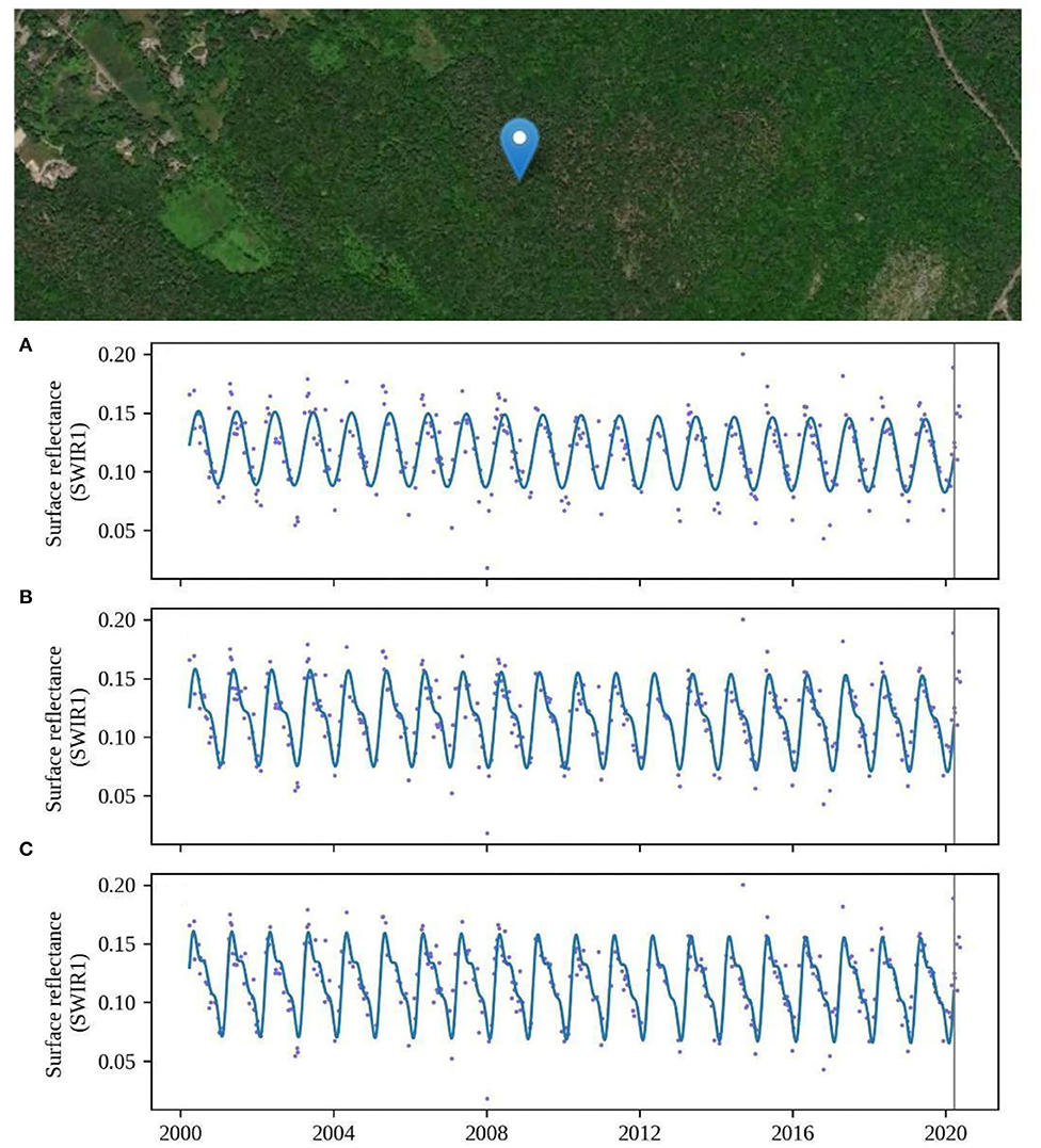
Figure 1. Landsat time series (dots) for the SWIR1 band, and the corresponding time segments detected by the CCDC algorithm, using different numbers of harmonics. (A) Time segment using only one harmonic (annual harmonic), (B) two harmonics (annual and six-month harmonics), and (C) three harmonics (annual, 6-, and 3-months harmonics). The pixel corresponds to a stable forest in the Blue Hills Reservation, in the commonwealth of Massachusetts, USA. Only a single spectral band is shown here, but CCDC fits harmonic models to all bands included in the analysis, which are specified by the user.

FIGURE 2

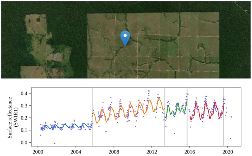
Figure 2. Time series for a pixel of Landsat observations (blue dots) for the SWIR1 band, and the corresponding time segments detected by the CCDC algorithm. Each shift of a time segment to the next depicts a detected change in the surface and can be characterized either as a change in land cover, land use, or land condition. This example from Rondônia, in Brazil, depicts a stable primary forest converted to agriculture circa 2006, and captures recurrent seasonal patterns of agricultural cycles that persist until today.

Another construct made possible through the use of CCDC results is a “synthetic image.” Once the harmonic regression models (i.e., time segments) have been fit by the CCDC algorithm, we can use them to estimate a value for a pixel at any time within the input data time range. This capability can be used for the creation of a “synthetic” image, which is simply the predicted value for all pixels for a given date (Zhu et al., 2015). For example, in Figure 2, an observation for a single pixel from a real Landsat image is represented by any of the blue dots, whereas the synthetic value for the same pixel would correspond to any value along the harmonic models, or their predicted value for the gaps between models. The use of synthetic images is discussed below in Section spatial data viewer.

The GEE implementation of the CCDC algorithm is data agnostic, meaning that in principle it can be applied to other multitemporal datasets other than Landsat, such as Sentinel-1 and -2. However, the algorithm was originally created to use Landsat observations, and most of the published research using CCDC has been applied to Landsat observations. For this reason, the applications shown here are demonstrated using Landsat-derived results and allow the user to interact with Collection 1 Landsat imagery and the products derived from the coefficients for the time segments fit by CCDC.

Graphical Interface Tools

The graphical interface tools we present here can be categorized in three groups:

1) Visualization and exploration tools.

2) Classification and mapping tools.

3) Area estimation and accuracy tools.

The tools were designed as standalone applications that can be used independently from each other, except for the Land cover tool, which requires the output of the Classification tool. Still, certain processes can be streamlined if all the apps are used together. For example, a user may be interested in generating a land cover map for a geographical area they are not familiar with. In this scenario the visualization tools could be used to explore the spatio-temporal land dynamics in that area. Once those are better understood, the user may collect training data and use it in the classification and mapping tool to produce maps of land cover change. Finally, the user may need to quantify the accuracy of such maps, or estimate areas of change with quantifiable uncertainty, for which they may use the last set of tools. However, considering that users may have different purposes for the tools that are not exclusively related to land cover mapping, only the core usage of each tool is described below, and independent case examples are presented in the results section.

Time Series Viewers

The time series viewers are simple interactive Earth Engine Apps that allow the user to explore series of Landsat observations for any pixel on the globe where such data are available. Cloudy or shadowed observations are filtered from the time series using the quality data flags contained in the Landsat collection images. The user can select the spectral band and time range to visualize and click on any point in the time series to load the corresponding image into the map viewer. The tools also show the time segments detected on-the-fly by the CCDC algorithm. Two versions of the tool are available. The first is the simple viewer (Figure 3), which can be found in this link: https://parevalo_bu.users.earthengine.app/view/quick-tstools. In this version, the options that the user can modify are minimal (i.e., time range and spectral band to visualize), as it was designed for use in mobile devices to facilitate the analysis of the landscape history directly in the field. The tool works on any mobile or desktop browser that is supported by Earth Engine Apps and runs CCDC using the default parameters. The second version of the tool is the “advanced” time series viewer (Figure 4), created for users who want to have more control on the parameters used for running CCDC and visualization. In addition to the capabilities described for the simple viewer, it is possible to modify the parameters to run the CCDC algorithm. The image visualization parameters or the range of spectral indices may also be modified. The tool also allows adding ancillary data stored as public assets to the map. The tool can be found here: https://parevalo_bu.users.earthengine.app/view/advanced-tstools.

FIGURE 3

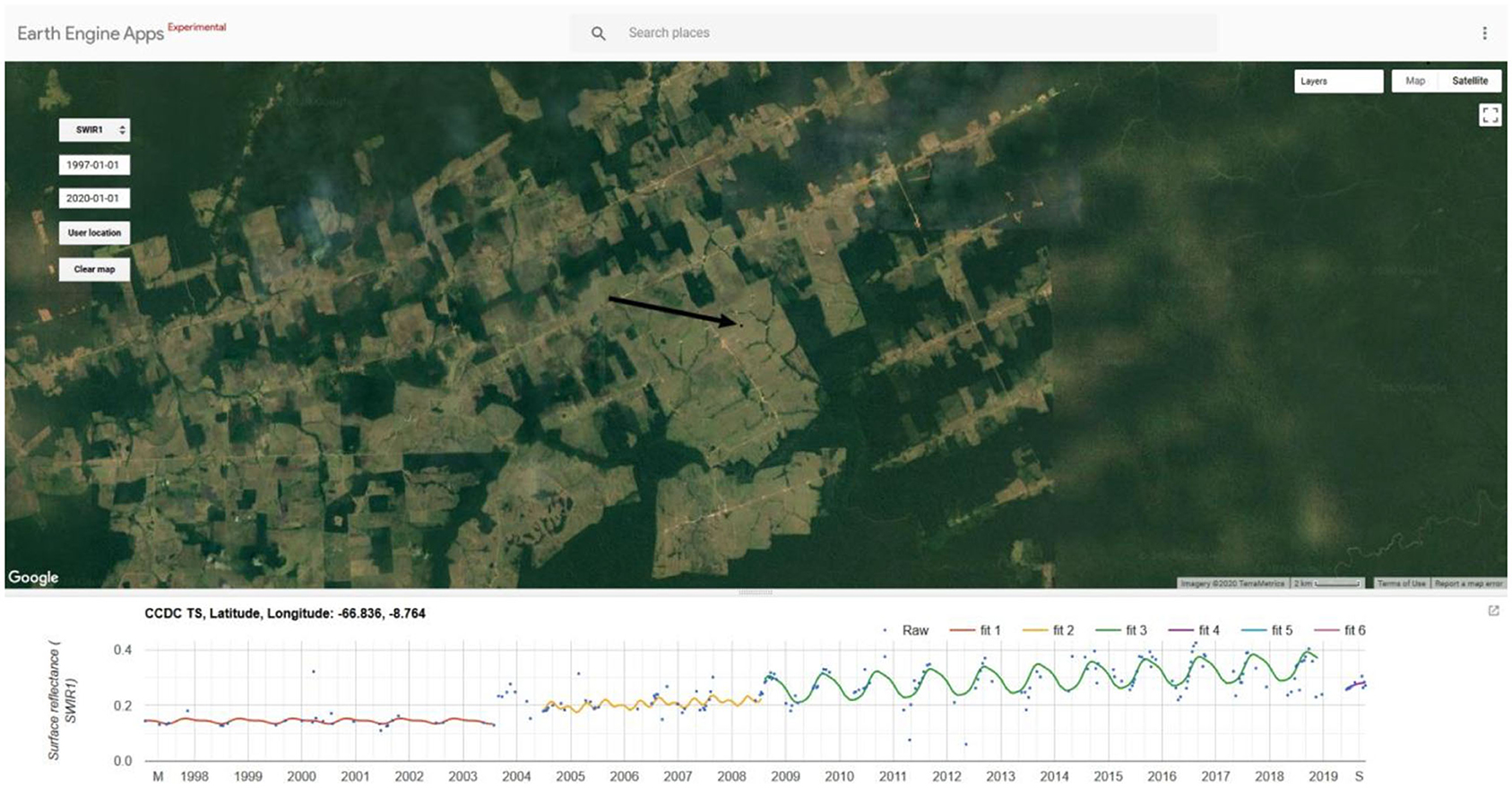
Figure 3. Screenshot of the Simple viewer tool displaying time series of Landsat observations (blue dots) for a given pixel (black arrow) and the associated time segments (“fit” lines) as detected by the CCDC algorithm. The time series captures a deforestation event in western Brazil in 2004 for that pixel and the surrounding areas, followed by the establishment of croplands.

FIGURE 4

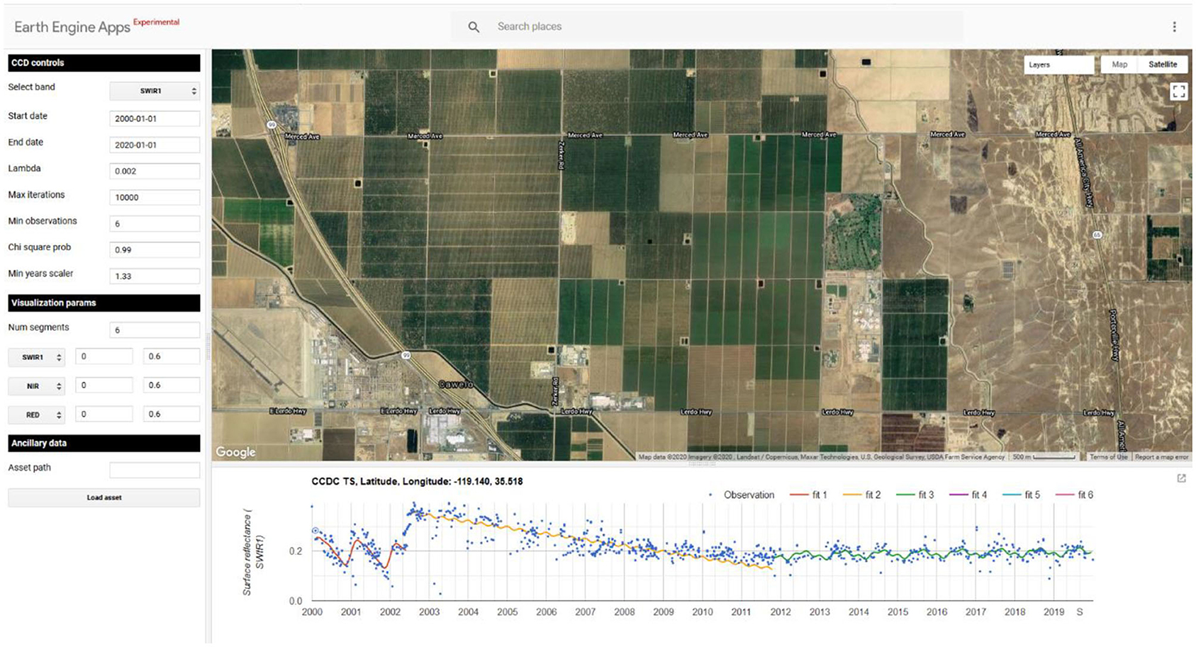
Figure 4. Screenshot of the Advanced time series tool showing the controls in the left panel. The time series of the clicked pixel represents long term agricultural cycles in California.

Spatial Data Viewer

The spatial data viewer tool (Figure 5) expands the capabilities of the time series viewers by allowing the user to spatially explore the coefficients of the time segments and the detected changes, as well as creating various Landsat derivatives. To use the core functionality of the tool, the user needs to specify the path to existing CCDC coefficients saved as GEE assets, either as the Earth Engine image that is created as the algorithm output, or as an Image Collection that contains one or more of those images. Once loaded, the tool enables the exploration of the following:

1) Model coefficients: as explained in Section CCDC algorithm, each time segment is defined by a set of coefficients: the intercept; the slope; and the harmonic terms of the regression model. These coefficients, as well as the RMSE, and the amplitude and phase of the harmonics, can be visualized using this tool. The user can add individual coefficients or color composites of coefficients to the map. Model coefficients, and quantities derived from them like the phase and amplitude of the harmonic models, can be used in a variety of ways. The most common use is in the classification step of CCDC where time segments are used as an input to the classification process. The classification process and the tool for its implementation are discussed below in Sections classification and spatial data viewer. However, coefficients and their derivatives have intrinsic value. For example, the amplitude of the harmonic regression is indicative of the magnitude of the changes in spectral bands seasonally, which could be related to deciduousness.

2) Synthetic images: the time segments can be used to predict the surface reflectance for any point in time within the time range of the input data. Imagery that is composed of predicted surface reflectance is referred to as “synthetic” imagery (Zhu et al., 2015), and can be generated using a color combination specified by the end user. Synthetic imagery can be generated for any day within the time range of the input data even in the absence of Landsat observations. These data represent a new kind of “derived” data product, as they are based on past Landsat observations, but are not themselves observations. They can be valuable and easy-to-use images as, by definition, they are free of the effects of clouds, cloud shadows, and snow. Additionally, they can capture the seasonality of locations when produced for multiple times of year, which can improve applications like image classification (Pasquarella et al., 2018).

3) Change information: for each pixel there is a variety of change information available. If changes (“breaks”) have been detected by the CCDC algorithm, there is information about the timing of the break, the magnitude of the break and the number of breaks. The magnitude of the break is calculated internally by the CCDC algorithm as the difference between the mean of the last five observations before the break and the mean of the first five observations after the break in any spectral band or index. The user can display the number of changes for a selected time period, the change with the largest magnitude (e.g., deforestation) and the time of the most recent or largest change.

FIGURE 5

Figure 5. Screenshot of the spatial data viewer interface, showing the amplitude of the temporal models for the SWIR1 band for the first day of 2001. Brighter values (yellow) represent locations with a more pronounced seasonality in the surface reflectance of the first Landsat SWIR band. At the bottom, the time series and fit temporal model for a clicked pixel in southeastern Australia. The right panel is used to load model coefficients, synthetic images or change layers. The left panel is used to change the parameters to run CCDC on-the-fly in a clicked pixel, and to control the visualization of Landsat images loaded by clicking on the time series chart.

The tool can be found at this link: https://parevalo_bu.users.earthengine.app/view/visualize-ccdc.

Classification

For classification, we provide two tools that can be used together for land cover and/or land use classification using the CCDC model parameters as predictor variables. The tools allow the creation of categorical maps, and the testing of input parameters without writing any code. The first tool, referred to here as the Classification Tool, allows users to classify the time segments created using the CCDC function in GEE. The user provides the path to the CCDC results (stored as Earth Engine Assets), training data (stored as an Earth Engine Feature Collection), and selects the machine learning classifier, predictor variables and study area to use. The user can select a country boundary to use as the study area or can draw the study area on the map. A list of the available predictor variables can be found in Table 1. The result is an N-band image corresponding to N time series segments. Since CCDC operates on the time series of every individual pixel, the start and end dates for the segments vary by pixel accordingly. Therefore, to extract a categorical map for a specific date, or change between multiple dates, a separate tool is required.

TABLE 1

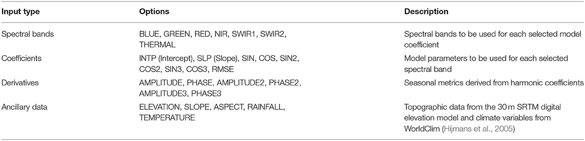
Table 1. List of currently available predictors for classification in the graphical user interface tool when all the Landsat bands are used.

The second tool, referred to here as the Land Cover Tool, allows users to create land cover or land use maps from the classified segments produced by the Classification Tool at any date in the study period. In addition, the Land Cover Tool allows users to specify a change layer, corresponding to conversion between one or multiple classes at a specific date to one or multiple other classes at a later date. The result is an N-band image corresponding to N-number of dates specified by the user, which can be visualized “on-the-fly” or exported as an image to an Earth Engine Asset, Google Cloud, or Google Drive (Figure 6). Unlike the tools described previously, the Classification and Land cover tools allow exporting the results as GEE assets. However, the Earth Engine App platform does not support exporting to GEE assets directly and therefore these tools cannot be distributed as “standalone” Earth Engine Apps but must be distributed as GEE scripts. For this reason, static links to the tools cannot be generated and need to be regenerated every time the code is updated. Up-to-date links to the tools can be found at https://gee-ccdc-tools.readthedocs.io.

FIGURE 6

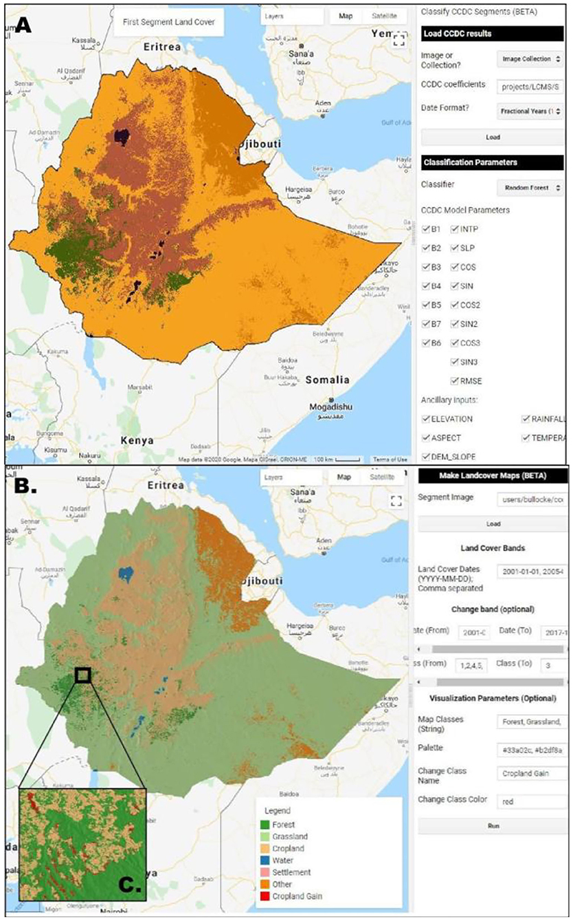
Figure 6. Screenshots of the Classification Tool used to classify CCDC segments for the country of Ethiopia (A), the Land Cover Tool which allows users to extract categorical maps, including maps of change, for any desired date or dates (B), and a subset of (B) that shows pixels classified as cropland gain due to displacement of forest (C).

AREA2: Area Estimation and Map Accuracy Assessment

Land cover and land change are important climate variables, and analyses of remote sensing data are often the only feasible way to determine the extent of these variables. Traditionally, maps constructed by classification of remote sensing data were used to quantify such variables by summing map units assigned to map classes (i.e., pixel counting). However, as emphasized in the literature, areas obtained in this way may be subject to bias due to classification errors (McRoberts, 2011; Olofsson et al., 2014; GFOI, 2016). Instead, a sample-based approach in which an unbiased estimator is applied to sample data for estimation of areas of interest is recommended. In this context, “unbiased” refers to a property of an estimator: the bias of an estimator $\widehat{\mu }$ of a population parameter μ is the difference between μ and the expected value of $\widehat{\mu }$ over all possible samples. Expressed mathematically, $\widehat{\mu }$ is unbiased if $Bias(\widehat{\mu })=E(\widehat{\mu })-\mu =0$ (Casella and Berger, 2002, p. 330).

Designing surveys, determining reference conditions on the land surface, and selecting, constructing and using appropriate estimators are all important but complex steps and decisions. To assist users navigating such choices, we have developed a toolkit titled AREA2 (ARea Estimation and Accuracy Assessment; “area two”). AREA2 (Bullock et al., 2020a) provides support for the three major components of an estimation protocol: sampling design, response design, and analysis (Stehman and Czaplewski, 1998).

The first component, sampling design, refers to the protocol for selecting a subset of population units (i.e., a sample) in the study area. AREA2 supports simple random (SRS) and systematic (SYS), stratified random (STR), and two-stage sampling. An important part of designing a survey is determining the sample size. With AREA2 we have implemented support for sample size determination using the variance estimators for SRS/SYS and STR designs [Equations 4.2 and 5.25 in Cochran (1977)] by specifying a target precision and then calculate the sample size required to achieve that precision.

Following the sampling design, the reference land surface condition needs recorded at each sample unit location by examining reference data. Good reference data have traditionally been commercial high-resolution data, aerial photos and field inventories but such data are costly and less than ideal for observing changes on the land surface through time. Reference data based on time series of observations have proven a powerful dataset for observing reference change conditions, especially when combined with high resolution imagery [e.g., Olofsson et al. (2016), Arévalo et al. (2020)]. Traditionally, compiling time series of Landsat data for sample locations was demanding as whole images in a series needed downloading and stacking before a time series could be extracted. Attempts were made to mitigate these issues, the best example being TimeSync which extracted annual “best image” chips of Landsat data at sample locations (Cohen et al., 2010). The viewer in AREA2 extracts time series of Landsat surface reflectance and various spectral indices from Google Earth Engine during a user specified time period (1982 at earliest). Clicking an observation in the series displays the associated Landsat image. The last step corresponds to the analysis, which includes protocols for estimating area, map accuracy and uncertainty (Olofsson et al., 2014). Central to the analysis is the estimator (preferably an unbiased estimator), which is a formula by which an estimate of a population parameter is calculated from the sample data (Cochran, 1977). Even though the estimator must correspond to the sampling design, there are usually more than one unbiased estimator to choose from and selecting the most efficient estimator in a given situation is often complex. Further, the implementation of the estimator (and the associated variance estimator) is not always straightforward, especially for complex designs such as two-stage sampling. AREA2 provides tutorials guiding users through the decisions, and supports the following estimators (the references provide the underlying mathematical frameworks and proof of unbiasedness):

• expansion estimators for simple random and systematic sampling (Cochran, 1977).

• stratified estimator for stratified random sampling (Cochran, 1977).

• post-stratified estimator for simple random and systematic sampling (Cochran, 1977).

• model-assisted regression estimator for stratified random sampling (Särndal et al., 2003).

• ratio estimator for stratified random sampling when the map classes that defined strata are different from the map classes in the final error matrix (Stehman, 2014).

• ratio estimator for use with two-stage sampling (Särndal et al., 2003).

AREA2 can be used with any categorical map, even if it was not created with the CCDC algorithm. For this reason it was created as a separate project, and the detailed documentation and tutorials are available at https://area2.readthedocs.io/.

Case Study for Land Cover Mapping and Area and Accuracy Estimation

We mapped land cover and land cover change due to expansion of built land in southeastern United States as a case study for using the classification tools and AREA2. We made use of previously developed training data from the NASA GLANCE project (http://sites.bu.edu/measures/) and reference data from LCMAP (Brown et al., 2020) to perform classification and assessment for the case study using the Classification tool. The study area consisted of the states of Florida, South Carolina, North Carolina, Louisiana, Mississippi, Georgia, Arkansas, Kentucky, and Alabama. The CCDC results used for this exercise correspond to preliminary CCDC outputs made available to us that are currently unavailable to the general public. However, a similar workflow can be carried out with any CCDC results run by a user, or by other publicly available or shared CCDC datasets. Following the steps of the Classification tool, we specified the path to the CCDC results and the training data, selected the features to be used in the classification (All of the inputs specified in Table 1), the classifier to use (a Random Forest classifier) and exported the resulting multi-band image containing a land cover class per time segment per pixel. These results were used as inputs to the Land Cover tool to map the expansion of the built class, referred to from now on as the “New Built” class. The change period selected for the creation of the change layer was 1999–2016, but any period between the original date range of the classification results can be studied.

After the change map finished loading “on-the-fly” in the tool map panel, we exported it as an asset to use in the AREA2 tool. Accuracy of the classification results were obtained using the reference sample, which was created independent on the training dataset. Since the reference sample was selected under a simple random sample design, it can be used to estimate map accuracy with AREA2 using the “direct estimator” available in the subfolder “3. Estimation” of the AREA2 repository.

Application Programming Interface

An API was built atop the GEE JavaScript API to facilitate custom operations with CCDC outputs and facilitate building the graphical tools presented here. The API currently contains the following modules:

1) Inputs: module to create Landsat, Sentinel 1 and 2 stacks for time series plotting, as well as the computation of indices derived from the optical sensors.

2) CCDC: module to manipulate the results from existing model runs done using Landsat observations, enabling the extraction of regression coefficients, the generation of synthetic images, and the extraction of time, magnitude and frequency of changes.

3) Classification: module to pre-process training data, classify CCDC coefficients and obtain land cover maps from them.

4) Dates: module to interact with dates in the formats required by the CCDC algorithm in Google Earth Engine.

5) Change: module to post-process the change results obtained from CCDC. Currently it contains functions to evaluate the presence of errors of omission and commission of change (Bullock et al., 2019).

Up to date links to access the API, the documentation, and a brief guide to use the core functions can be found in this link: https://gee-ccdc-tools.readthedocs.io.

Results

We illustrate the varied usage and multiple applications of the tools presented above with three examples. The time series viewers are demonstrated using a localized change example in Quincy, Massachusetts. The CCDC visualization tool is demonstrated using much larger fire events in northern Argentina. Finally, an example of land cover and land cover change mapping are shown for the Southeastern USA, followed by the estimation of accuracies and change areas. The different areas were selected to demonstrate how the tools can aid in the understanding of land change at different scales, and how they can be used in different geographical areas with varying levels of data coverage and drivers of change.

Time Series Viewers

The Simple Time Series Viewer has been used in university courses (at Boston University) to visualize the history of the landscape in situ through a mobile phone. On field trips, students were able to interact with Landsat time series plots, allowing them to address questions related to the landscape history at their immediate location. One of such locations was in Quincy, Massachusetts. Students accessed the tool through their mobile phones, located themselves in the map using the “User location” button, and clicked on the map to reveal the Landsat time series, as well as the time segments detected by CCDC on the fly. In the example shown in Figure 7, two temporal segments are detected by CCDC: one starting in 1997 and ending in 2004, and another starting in 2005 and ending in 2020. The first segment represents the forested area that was cleared to make space for housing, represented by the second segment. The time range between segments circa 2005 corresponds to the transition between these two land cover classes, when the CCDC algorithm waits for more stable observations to start fitting a new segment.

FIGURE 7

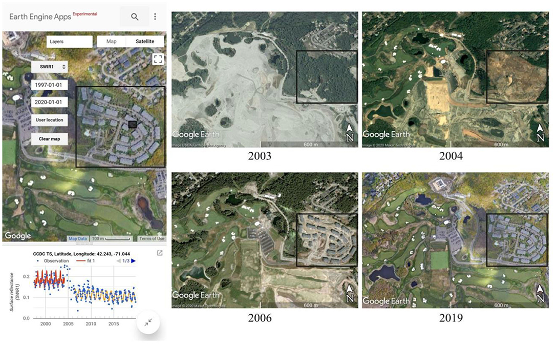
Figure 7. Left panel: interface of the Simple time series viewer as seen in a mobile phone. The smaller square shows the clicked location on the map, with the corresponding Landsat time series and CCDC segments show below. Right panels: Multi-temporal high-resolution images of the area shown for reference, highlighting the conversion from forested area to developed.

The ability to easily explore historical imagery on mobile phones in-situ to make sense of the land changes over time is a groundbreaking advancement made possible by Google Earth Engine and its Apps platform. More complex temporal dynamics are easier to investigate using the full time series viewer on a larger browser, such as a tablet of laptop. Using the same example presented before, the Advanced time series viewer can be used to investigate other changes in the area in more detail. Figure 8 shows the time series for a pixel located in the golf course visible in the western side of Figure 7. This area, formerly a covered landfill, was transformed into a golf course during the early 2000's using the material extracted from a mega-construction project in the Boston area (commonly referred to as the “Big Dig”). The time series in Figure 8 show three segments representing these land covers and transitions: grass vegetation (first segment), followed by a complete removal and the landscape transformation that took place between 1998 and 2006 (second segment), and then the establishment of permanent, irrigated grass for the golf course around 2007 (third segment).

FIGURE 8

Figure 8. Landsat time series showing the transformation from landfill to golf course. Hovering on the observations with the pointer shows their date and corresponding value. Clicking on them will load the corresponding Landsat image, using the visualization parameters for Red-Green-Blue (RGB) composite in the left panel.

Spatial Data Viewer

The spatial data viewer tool is demonstrated using an example from northern Argentina. CCDC results for the period between 1985 and 2000 are loaded in the tool, and the “Create synthetic image” section on the right panel is used to create a predicted image for the date 1996-01-01, to use as a snapshot of the landscape. Fire scars are evident in the image, showing non-geometric patterns of change compared to nearby agriculture and roads (Figure 9). After changing the band selection on the left panel to “NBR” (Normalized Burned Ratio) and clicking anywhere in the fire scar, the time series loaded in the bottom panel show negative values circa 1996 that suggest the occurrence of a fire event. To obtain a map that shows the approximate time of change for the entire area, the “Visualize section” on the right panel can be used to select a period centered in 1996 (e.g., 1994–1997), a spectral band to visualize the magnitude of the change detected by CCDC (i.e., SWIR1) and the desired change layer, in this case, the “Time of maximum magnitude of change.” The loaded image shows a clear fire even that happened circa 1994 for this fire scar, as well as the timing for other change events in the surrounding areas.

FIGURE 9

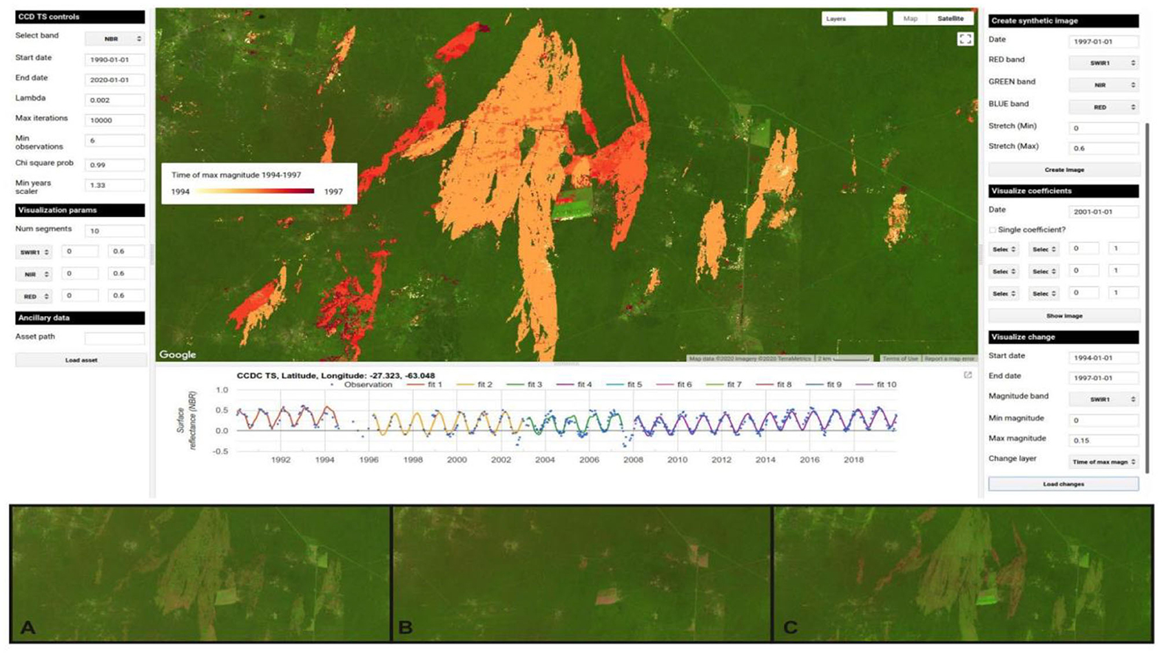
Figure 9. Interface of the spatial data viewer (upper panel) showing the time of maximum magnitude of change between 1994 and 1997 in this area, revealing the timing of fire events. The change layer was created using the “Visualize change” section on the bottom of the right panel. The time series in the bottom panel are displayed following the settings on the left panel. Insets below the screenshot show: (A) The synthetic image for the first day of 1997; (B) A surface reflectance Landsat image prior to the fire even (1994-02-07), loaded by clicking on the corresponding observation in the time series chart; (C) a surface reflectance Landsat image after the fire event (1996-03-16) loaded in the same way as the prior image. Images are shown in RGB color combination corresponding to the SWIR1, NIR, and Red bands, respectively, as set in the “Visualization params” section on the left panel.

Classification and Estimation of Area and Accuracy

The results consisted of: (1) Classified time segments between 2000 and 2016 for the study region, equivalent to land cover maps at 30 m resolution for any given date between that period, (2) a single land cover change map showing stable classes and the “New built” change class between 2000 and 206, and (3) estimates of area and accuracy with standard errors for the classes in the land cover change map. Figure 10 highlights the “New Built” class for two subsets in North Carolina and Tennessee. The results are displayed using a custom palette, defined manually in the Visualization Parameters of the Land Cover tool and represented in the map as a legend. The map contains seven stable classes (Water, Snow/Ice, Built, Bare, Forest, Shrub, and Herbaceous) and the change class of interest (New Built). It should be noted that the results in Figure 10 are shown as created “on-the-fly” in the Land cover tool but they must be exported as assets to be used in the AREA2 tools. The runtime to export the classified time segments as an Earth Engine asset from the Classification tool was 5 h, while the runtime to export the change map from the Land cover tool was 10 h, but these times will vary depending on several factors, including the area extent, pixel size, number of input features and time segments, and other factors inherent to GEE.

FIGURE 10

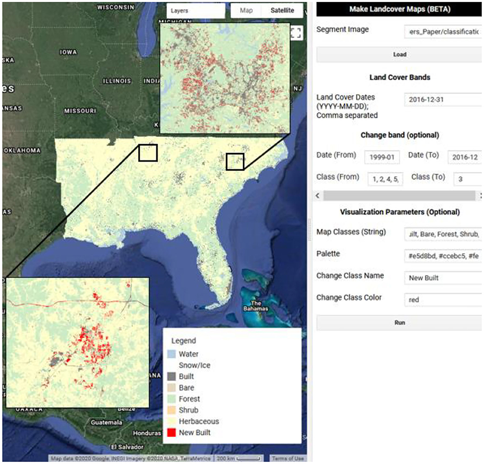
Figure 10. Screenshot of the Land Cover Tool used to display the land cover classification at the end of 2016 and conversion to Built land (“New Built”). Insets detailing some of the largest change areas were manually overlayed for display in this figure.

Area and accuracy estimates produced by AREA2 are shown in Tables 2, 3. The Overall accuracy of the map was 80% and the Producer's and User's accuracies of the “New Built” class were 40 and 15%, respectively. The sample-based estimates revealed 507,000 ha of conversion to Built during the study period. The predominant land cover class at the end of the study period in 2016 was the Tree class, representing 60% of the study area, or 71,142,000 ha.

TABLE 2

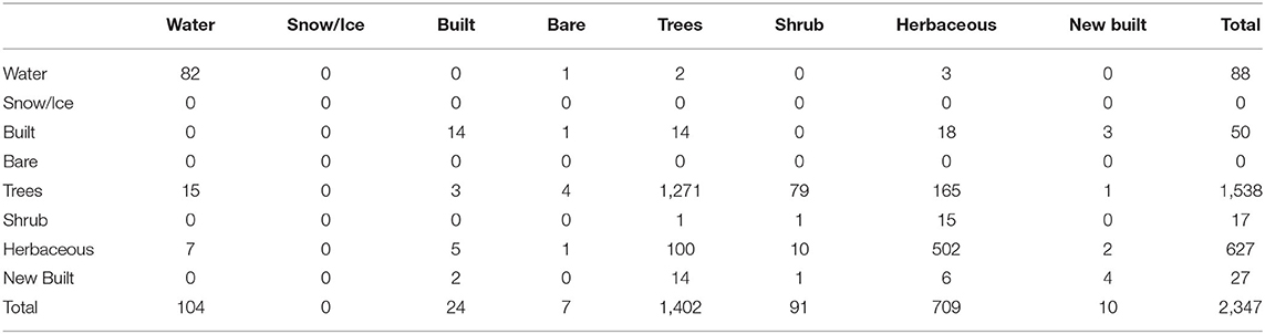
Table 2. Confusion matrix expressed as sample counts with reference observations in the columns and map values in rows.

TABLE 3

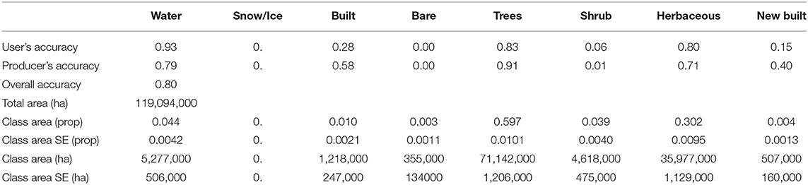
Table 3. Accuracies and estimated areas with standard errors (SE) as proportion of the total area (prop) and in units of ha.

Discussion

The functionality of the tools presented in this paper is intended to simplify user interaction with time series of Landsat data, and to provide a system to explore and extract valuable information from the data, such as multi-temporal metrics and long term landscape change through the use of the CCDC algorithm. The use of CCDC by the broader community has been historically hampered by storage and preprocessing demands, and computational complexity. With the emergence of cloud computing and public repositories of satellite data, we have an opportunity to expand user access to CCDC outputs. To achieve broader access, we have developed a set of tools with graphical interfaces that enable a range of workflows from simple exploratory analysis to production of more complex products In essence, the tools presented here provide a new way for the public to interact with time series of satellite data with minimal effort. Our hope is that these tools will lead to a broader understanding of the way Earth is changing as well as an appreciation of the value of sustained satellite measurements over long time periods.

The tools presented here facilitate the monitoring and estimation of land change and associated carbon emission by removing the challenges such as the processing of large volumes of Landsat imagery, screening of noise and cloud/cloud shadow, and demands on storage space and computational power. Graphical user interfaces and API functionality, coupled with tutorials and documentation, provide sufficient flexibility to accommodate national and local circumstances and suit users with different levels of technical expertise. For example, users with little or no experience with the CCDC algorithm can use the exploratory tools to get familiarized with the basic concepts surrounding its use, such as the “time segments.” Users that are more familiar with the outputs of the algorithm can visualize model coefficients or interact with them without having to process the CCDC results themselves. Similarly, countries without national maps of land cover change can start by exploring the time series data in their region to assess the suitability of the CCDC algorithm to capture change patterns of interest. Countries with higher image-processing capabilities can make use of the API to extract CCDC-derived products and process them with their own custom-made functionality. Furthermore, the availability of tools to create stratifications, assess the accuracy of map products, and estimate areas of change can benefit both new users creating preliminary maps, or experienced users with existing maps, even if created using different algorithms and tools.

An example that illustrates the use of CCDC outputs for monitoring, along with sample-based estimation, of multiple land cover transitions in support of REDD+ reporting was presented by Arévalo et al. (2020). The study was conducted before the availability of the CCDC algorithm in GEE, and required manual downloading and stacking of more than 5,000 Landsat images. Visualization of time series for a single pixel was possible only after the stacking process was complete, and the CCDC algorithm had to be run for each WRS-2 path and row scene separately; this translated into running the model at least 25 times to cover the Colombian Amazon. Once the time segments were classified, each Landsat footprint was mapped separately, resulting in the need to merge individual maps into a coherent, seamless mosaic. This cumbersome workflow could now be completely reproduced in GEE using the API and tools presented here, without the need for extensive pre- and post-processing. The gain in efficiency is illustrated in the example presented in Section classification and estimation of area and accuracy for the Southeastern USA. Even though the study area was larger than the area mapped in Arévalo et al. (2020), the process was completed in just 15 h. Furthermore, the ability to inspect time series and visualize classification results on-the-fly allows for time-efficient quality control that is likely to result in improved maps.

Another example illustrating how the presented tools can accelerate map creation, quality control, and assessment processes is provided by a recent capacity-building collaboration with the Government of Zambia via SilvaCarbon. In this collaboration, we assisted Zambia's forestry department in using a set of existing training datasets to create land cover change maps, and to assess and improve their accuracy. First, we used the tools for time series visualization to determine if the land cover changes of interest were readily captured by the CCDC algorithm. This step was accomplished using the function in the Advanced Spatial Data Viewer that allows visualization of the breaks found by CCDC. Second, we wanted to test which of the various training datasets produced the most accurate map. The use of the CCDC and Classification modules in the API tools enabled iterative production of temporally consistent maps of land cover and land cover change for the entire country using each of the training datasets (Figure 11). Finally, the accuracies of the newly created maps were estimated using AREA2 to determine which of the training datasets produced the most accurate map. An important aspect of the Zambia example is capacity building; all steps were completed in just a few days of work with us the authors, using the tools in the beginning of the workshop but after only a day or two, the participants from the Zambia Forestry Department were producing the maps, inspecting the results and estimating accuracy measures. The example illustrates the potential of the presented tools to enable local practitioners in tropical countries to use advanced environmental remote sensing in support of climate science, and ultimately climate mitigation.

FIGURE 11

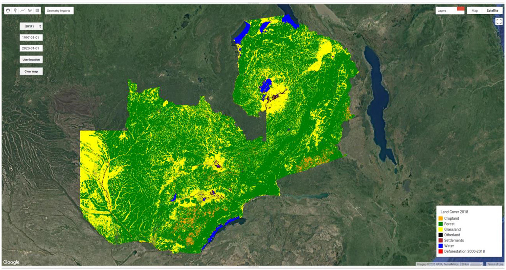
Figure 11. Screenshot of an example land cover and change map of the country of Zambia created iteratively with the tools and functions included in the API.

The tools and functionality available in the API are currently being used as part of the mapping and assessment procedures for the Global Land Cover mapping and Estimation (GLanCE) project, a NASA MEaSURES project at Boston University (http://sites.bu.edu/measures/). GLanCE will provide a data record of twenty-first century global land cover, land use and land cover change at 30 m resolution. The intent is to provide global maps of land cover and land cover change with estimates of area and map accuracy. A similar effort was carried out for the United States by the USGS developed a system for operational monitoring of land change as part of its LCMAP initiative. To implement CCDC at a national scale, they built the computing infrastructure necessary to process the entire Landsat archive for the United States using CCDC, as well as implement similar kinds of tools to those presented in this paper to convert CCDC results to a suite of 10 operational products related to land cover and land cover change (Brown et al., 2020). The resulting global maps produced by the GlanCE project are expected to provide baseline characterization of the ways the land surface is changing and will aid in the characterization of biophysical properties of the Earth's land surface. We also expect the resulting products to contribute to model-based investigations that require land cover and change information, such as carbon balance models. The deliverables are complex and can be thought of as a database of time segments with a set of attributes in space and time. This complexity poses a potential hurdle for users, but we envision that the presented tools will allow the creation of maps of land cover and land cover change for any region in the world where the required data is available.

Once maps have been created, guidance is needed for how to use maps in an inference framework to estimate areas and map accuracy. AREA2 was designed to guide users through the decisions involved in the estimation process and to relieve users of the burden of constructing estimators. The tools in AREA2 have been used for this purpose at capacity building workshops in Costa Rica, Peru, and other countries, and for sample interpretation and area estimation in Guatemala as part of efforts to estimate forest disturbance in Guatemala's protected areas (Bullock et al., 2020b). As it becomes easier to create maps with existing and new tools like the ones presented here, it is crucial to assess and report the accuracy of such products. For this reason, we envision AREA2 as an integrated part of a mapping workflow that uses advanced remote-sensing products, such as those derived from the CCDC algorithm.

Some considerations and limitations must be considered when using the tools and functions presented in this paper. First, they are provided free of charge “as-is” without any warranty or support, and they are subject to change at any time. We expect to continue improving and adding functionality to the tools, especially to the time series and classification tools, for at least another year or as long as it is feasible. The AREA2 repository will continue to be monitored for potential coding issues. Users are welcome to contribute to the development of new functionality or provide suggestions. Due to the current limitations for multi-user collaboration in a GEE repository, we have created a GitHub repository with a copy of the most recent and stable version of the API and tools and we will update it periodically to ensure the proper archival of new functionality. The repository is located at: https://github.com/parevalo/gee-ccdc-tools. Second, while the Google Earth Engine team has been supportive of the development of these tools, they are not produced or endorsed by Google. Similarly, this paper does not intend to serve as the official description of the GEE implementation of CCDC. Finally, the tools in their current iteration have not been designed or tested with CCDC results from sensors other than Landsat. However, our end goal is to provide a set of tools that are sensor agnostic. Web links to other tools designed to explore Sentinel data will be published on the website referenced previously as soon as they become available.

Finally, while a primary objective of the tools presented here is to aid in land cover mapping, various other applications of benefit to users interested in land surface dynamics and their effect on climate are possible. For example, the frequency and magnitude of change events detected by the algorithm could be used to determine the timing of forest loss events or agricultural cycles. The variability in the surface reflectance could be visualized via the RMSE of the time segments. Seasonality information contained in the amplitude and phase of the harmonic terms of the regression could be used to study vegetation phenology as well as mapping of deciduousness. Long- and short-term trends in land cover condition, as captured by the slopes of the time segments, could be analyzed to identify vegetation recovery. Cloud-free synthetic images could benefit studies of the land surface, particularly in areas with low data density or high cloud occurrence. Previously published studies and algorithms that make use of CCDC outputs could be implemented for larger study areas. For example, a carbon bookkeeping model recently implemented to operate at the Landsat pixel scale using CCDC results (Tang et al., 2020) could be implemented and applied to a larger geographical area, such as the pantropics, using the tools we present here. Furthermore, current efforts to use CCDC results and the presented API to improve the mapping of biomass density in the Amazon basin by using the information contained in the temporal and spatial domains are other examples of how the tools could enable the study of land processes and properties directly related to climate. We believe that the tools presented in this paper will make these and other types of analyses more accessible to a broader set of scientists.

Conclusion

We have created a set of tools that facilitate the exploration of time series of Landsat observations and the time segments identified by CCDC. We believe these tools will simplify the visualization of time series of Landsat observations, facilitate the exploration of CCDC coefficients and derivatives, and streamline the creation of land cover and land cover change maps, as well as the estimation of areas and accuracies. By removing some of the barriers that prevent users from tapping into the information contained in time series of Landsat observations, we expect that users will extract new useful information that can be directly applied to climate science. Updated documentation and current links to the tools and API are available at https://gee-ccdc-tools.readthedocs.io.

Data Availability Statement

The original contributions presented in the study are included in the article/supplementary materials, further inquiries can be directed to the corresponding author/s.

Author Contributions

PA and EB implemented the tools. All authors conceived and contributed to the text.

Funding

PO and PA were funded by support from the NASA Carbon Monitoring System, grant NNX16AP26G (PI: Pontus Olofsson). PA was also funded through NASA research grant 80NSSC18K0994 (PI: Mark Friedl). EB was funded through NASA research grant 80NSSC18K0994 (PI: Mark Friedl) and SERVIR Applied Science Team grant NNH16AD021 (PI: Sean Healey). CW was funded by support from the USGS/NASA Landsat Science Team. Parts of the code required to visualize the time series and time segments, as well as re-processing of CCDC outputs were provided by Noel Gorelick and Zhiqiang Yang.

Conflict of Interest

The authors declare that the research was conducted in the absence of any commercial or financial relationships that could be construed as a potential conflict of interest.

Acknowledgments

We thank the Google Earth Engine 2018 Summit hackathon participants for the valuable contributions to the AREA2 concept.

References

Appel, M. (2020). bfast2/geeMonitor. bfast2 Available online at: https://github.com/bfast2/geeMonitor (accessed September 15, 2020).

Arévalo, P., and Bullock, E. (2020). gee-ccdc-tools. Zenodo. doi: 10.5281/zenodo.4029548

CrossRef Full Text

Arévalo, P., Olofsson, P., and Woodcock, C. E. (2020). Continuous monitoring of land change activities and post-disturbance dynamics from Landsat time series: a test methodology for REDD+ reporting. Remote Sens. Environ. 238:111051. doi: 10.1016/j.rse.2019.01.013

CrossRef Full Text | Google Scholar

Bolton, D. K., and Friedl, M. A. (2013). Forecasting crop yield using remotely sensed vegetation indices and crop phenology metrics. Agricult. For. Meteorol. 173, 74–84. doi: 10.1016/j.agrformet.2013.01.007

CrossRef Full Text | Google Scholar

Brown, J. F., Tollerud, H. J., Barber, C. P., Zhou, Q., Dwyer, J. L., Vogelmann, J. E., et al. (2020). Lessons learned implementing an operational continuous United States national land change monitoring capability: the Land Change Monitoring, Assessment, and Projection (LCMAP) approach. Remote Sens. Environ. 238:111356. doi: 10.1016/j.rse.2019.111356

CrossRef Full Text | Google Scholar

Bullock, E., Arévalo, P., Olofsson, P., and Singh, D. (2020a). Area Estimation and Accuracy Assessment Toolbox (AREA2). doi: 10.5281/zenodo.3451451

CrossRef Full Text

Bullock, E. L., Nolte, C., Segovia, A. L. R., and Woodcock, C. E. (2020b). Ongoing forest disturbance in Guatemala's protected areas. Remote Sens. Ecol. Conserv. 6, 141–152. doi: 10.1002/rse2.130

PubMed Abstract | CrossRef Full Text | Google Scholar

Bullock, E. L., Woodcock, C. E., and Holden, C. E. (2019). Improved change monitoring using an ensemble of time series algorithms. Remote Sens. Environ. 238:111165. doi: 10.1016/j.rse.2019.04.018

CrossRef Full Text | Google Scholar

Casella, G., and Berger, R. L. (2002). Statistical Inference. 2nd Ed. Australia: Duxbury-Thomson Learning.

Google Scholar

Claverie, M., Ju, J., Masek, J. G., Dungan, J. L., Vermote, E. F., Roger, J.-C., et al. (2018). The harmonized landsat and sentinel-2 surface reflectance data set. Remote Sens. Environ. 219, 145–161. doi: 10.1016/j.rse.2018.09.002

CrossRef Full Text | Google Scholar

Cochran, W. G. (1977). Sampling Techniques. 3rd Ed. New York, NY: John Wiley & Sons

Google Scholar

Cohen, W. B., Yang, Z., and Kennedy, R. (2010). Detecting trends in forest disturbance and recovery using yearly Landsat time series: 2. TimeSync—tools for calibration and validation. Remote Sens. Environ. 114, 2911–2924. doi: 10.1016/j.rse.2010.07.010

CrossRef Full Text | Google Scholar

Coppin, P. R., and Bauer, M. E. (1996). Digital change detection in forest ecosystems with remote sensing imagery. Remote Sens. Rev. 13, 207–234. doi: 10.1080/02757259609532305

CrossRef Full Text | Google Scholar

Dragoni, D., and Rahman, A. F. (2012). Trends in fall phenology across the deciduous forests of the Eastern USA. Agricult. For. Meteorol. 157, 96–105. doi: 10.1016/j.agrformet.2012.01.019

CrossRef Full Text | Google Scholar

Ganguly, S., Friedl, M. A., Tan, B., Zhang, X., and Verma, M. (2010). Land surface phenology from MODIS: characterization of the Collection 5 global land cover dynamics product. Remote Sens. Environ. 114, 1805–1816. doi: 10.1016/j.rse.2010.04.005

CrossRef Full Text | Google Scholar

GFOI (2016). Integrating remote-sensing and ground-based observations for estimation of emissions and removals of greenhouse gases in forests: Methods and Guidance from the Global Forest Observations Initiative. 2nd Ed. Rome: Food and Agriculture Organization of the United Nations Available online at: https://www.reddcompass.org/documents/184/0/GFOI-MGD-2.0-english.pdf/8f744ee0-d387-4376-9c9b-91eccbd7f54a (accessed July 14, 2016).

Google Scholar

Giglio, L., Boschetti, L., Roy, D. P., Humber, M. L., and Justice, C. O. (2018). The collection 6 MODIS burned area mapping algorithm and product. Remote Sens. Environ. 217, 72–85. doi: 10.1016/j.rse.2018.08.005

PubMed Abstract | CrossRef Full Text | Google Scholar

Goetz, S. J., Hansen, M., Houghton, R. A., Walker, W., Laporte, N., and Busch, J. (2015). Measurement and monitoring needs, capabilities and potential for addressing reduced emissions from deforestation and forest degradation under REDD+. Environ. Res. Lett. 10:123001. doi: 10.1088/1748-9326/10/12/123001

CrossRef Full Text | Google Scholar

Google (2020). Google Earth Engine API Documentation: ee.Algorithms.TemporalSegmentation.Ccdc. Google Developers. Available online at: https://developers.google.com/earth-engine/apidocs/ee-algorithms-temporalsegmentation-ccdc (accessed August 14, 2020).

Gorelick, N., Hancher, M., Dixon, M., Ilyushchenko, S., Thau, D., and Moore, R. (2017). Google earth engine: planetary-scale geospatial analysis for everyone. Remote Sens. Environ. 202, 18–27. doi: 10.1016/j.rse.2017.06.031

CrossRef Full Text | Google Scholar

Hansen, M. C., and Loveland, T. R. (2012). A review of large area monitoring of land cover change using Landsat data. Remote Sens. Environ. 122, 66–74. doi: 10.1016/j.rse.2011.08.024

CrossRef Full Text | Google Scholar

Henebry, G. M., and Beurs, K. M. (2013). Remote sensing of land surface phenology: a prospectus. Phenology 385–411. doi: 10.1007/978-94-007-6925-0_21

CrossRef Full Text | Google Scholar

Hijmans, R. J., Cameron, S. E., Parra, J. L., Jones, P. G., and Jarvis, A. (2005). Very high resolution interpolated climate surfaces for global land areas. Int. J. Climatol. 25, 1965–1978. doi: 10.1002/joc.1276

CrossRef Full Text | Google Scholar

Holden, C. (2017). ceholden/TSTools: TSTools: v1.2.0. Zenodo. doi: 10.5281/zenodo.267110

CrossRef Full Text

Houghton, R. A., House, J. I., Pongratz, J., van der Werf, G. R., DeFries, R. S., Hansen, M. C., et al. (2012). Carbon emissions from land use and land-cover change. Biogeosciences 9, 5125–5142. doi: 10.5194/bg-9-5125-2012

CrossRef Full Text | Google Scholar

Houghton, R. A., and Nassikas, A. A. (2017). Global and regional fluxes of carbon from land use and land cover change 1850–2015. Glob. Biogeochem. Cycles 31, 456–472. doi: 10.1002/2016GB005546

CrossRef Full Text | Google Scholar

Huang, C., Goward, S. N., Masek, J. G., Thomas, N., Zhu, Z., and Vogelmann, J. E. (2010). An automated approach for reconstructing recent forest disturbance history using dense Landsat time series stacks. Remote Sens. Environ. 114, 183–198. doi: 10.1016/j.rse.2009.08.017

CrossRef Full Text | Google Scholar

Hughes, M. J., Kaylor, S. D., and Hayes, D. J. (2017). Patch-based forest change detection from landsat time series. Forests 8:166. doi: 10.3390/f8050166

CrossRef Full Text | Google Scholar

Kennedy, R. E., Yang, Z., and Cohen, W. B. (2010). Detecting trends in forest disturbance and recovery using yearly Landsat time series: 1. LandTrendr—temporal segmentation algorithms. Remote Sens. Environ. 114, 2897–2910. doi: 10.1016/j.rse.2010.07.008

CrossRef Full Text | Google Scholar

McRoberts, R. E. (2011). Satellite image-based maps: scientific inference or pretty pictures? Remote Sens. Environ. 115, 715–724. doi: 10.1016/j.rse.2010.10.013

CrossRef Full Text | Google Scholar

Moon, M., Zhang, X., Henebry, G. M., Liu, L., Gray, J. M., Melaas, E. K., et al. (2019). Long-term continuity in land surface phenology measurements: a comparative assessment of the MODIS land cover dynamics and VIIRS land surface phenology products. Remote Sens. Environ. 226, 74–92. doi: 10.1016/j.rse.2019.03.034

CrossRef Full Text | Google Scholar

Morisette, J. T., Richardson, A. D., Knapp, A. K., Fisher, J. I., Graham, E. A., Abatzoglou, J., et al. (2009). Tracking the rhythm of the seasons in the face of global change: phenological research in the 21st century. Front. Ecol. Environ. 7:217. doi: 10.1890/070217

CrossRef Full Text | Google Scholar

Olander, L. P., Gibbs, H. K., Steininger, M., Swenson, J. J., and Murray, B. C. (2008). Reference scenarios for deforestation and forest degradation in support of REDD: a review of data and methods. Environ. Res. Lett. 3:025011. doi: 10.1088/1748-9326/3/2/025011

CrossRef Full Text | Google Scholar

Olofsson, P., Foody, G. M., Herold, M., Stehman, S. V., Woodcock, C. E., and Wulder, M. A. (2014). Good practices for estimating area and assessing accuracy of land change. Remote Sens. Environ. 148, 42–57. doi: 10.1016/j.rse.2014.02.015

CrossRef Full Text | Google Scholar

Olofsson, P., Holden, C. E., Bullock, E. L., and Woodcock, C. E. (2016). Time series analysis of satellite data reveals continuous deforestation of New England since the 1980s. Environ. Res. Lett. 11:064002. doi: 10.1088/1748-9326/11/6/064002

CrossRef Full Text | Google Scholar

Pasquarella, V. J., Holden, C. E., and Woodcock, C. E. (2018). Improved mapping of forest type using spectral-temporal Landsat features. Remote Sens. Environ. 210, 193–207. doi: 10.1016/j.rse.2018.02.064

CrossRef Full Text | Google Scholar

Särndal, C.-E., Swensson, B., and Wretman, J. (2003). Model Assisted Survey Sampling. New York, NY; Berlin; Heidelberg: Springer Science & Business Media.

Google Scholar

Schwartz, M. D., Ahas, R., and Aasa, A. (2006). Onset of spring starting earlier across the Northern Hemisphere. Glob. Chang. Biol. 12, 343–351. doi: 10.1111/j.1365-2486.2005.01097.x

CrossRef Full Text | Google Scholar

Sellers, P. J., Dickinson, R. E., Randall, D. A., Betts, A. K., Hall, F. G., Berry, J. A., et al. (1997). Modeling the exchanges of energy, water, and carbon between continents and the atmosphere. Science 275, 502–509. doi: 10.1126/science.275.5299.502

PubMed Abstract | CrossRef Full Text | Google Scholar

Stehman, S. V. (2014). Estimating area and map accuracy for stratified random sampling when the strata are different from the map classes. Int. J. Remote Sens. 35, 4923–4939. doi: 10.1080/01431161.2014.930207

CrossRef Full Text | Google Scholar

Stehman, S. V., and Czaplewski, R. L. (1998). Design and analysis for thematic map accuracy assessment: fundamental principles. Remote Sens. Environ. 64, 331–344. doi: 10.1016/S0034-4257(98)00010-8

CrossRef Full Text | Google Scholar

Tang, X., Hutyra, L. R., Arévalo, P., Baccini, A., Woodcock, C. E., and Olofsson, P. (2020). Spatiotemporal tracking of carbon emissions and uptake using time series analysis of Landsat data: a spatially explicit carbon bookkeeping model. Sci. Total Environ. 720:137409. doi: 10.1016/j.scitotenv.2020.137409

PubMed Abstract | CrossRef Full Text | Google Scholar

USGS (2018). Landsat Collections. Reston, VA: US Geological Survey.

Verbesselt, J., Hyndman, R., Newnham, G., and Culvenor, D. (2010). Detecting trend and seasonal changes in satellite image time series. Remote Sens. Environ. 114, 106–115. doi: 10.1016/j.rse.2009.08.014

CrossRef Full Text | Google Scholar

Vermote, E., Justice, C., Claverie, M., and Franch, B. (2016). Preliminary analysis of the performance of the Landsat 8/OLI land surface reflectance product. Remote Sens. Environ. 185, 46–56. doi: 10.1016/j.rse.2016.04.008

PubMed Abstract | CrossRef Full Text | Google Scholar

WMO (2020). About Essential Climate Variables. Available online at: https://gcos.wmo.int/en/essential-climate-variables/about (accessed September 11, 2020).

Woodcock, C. E., Loveland, T. R., Herold, M., and Bauer, M. E. (2020). Transitioning from change detection to monitoring with remote sensing: a paradigm shift. Remote Sens. Environ. 238:111558. doi: 10.1016/j.rse.2019.111558

CrossRef Full Text | Google Scholar

Zhu, Z. (2017). Change detection using landsat time series: a review of frequencies, preprocessing, algorithms, and applications. ISPRS J. Photogr. Remote Sens. 130, 370–384. doi: 10.1016/j.isprsjprs.2017.06.013

CrossRef Full Text | Google Scholar

Zhu, Z., and Woodcock, C. E. (2014). Automated cloud, cloud shadow, and snow detection in multitemporal landsat data: an algorithm designed specifically for monitoring land cover change. Remote Sens. Environ. 152, 217–234. doi: 10.1016/j.rse.2014.06.012

CrossRef Full Text | Google Scholar

Zhu, Z., Woodcock, C. E., Holden, C., and Yang, Z. (2015). Generating synthetic Landsat images based on all available Landsat data: predicting Landsat surface reflectance at any given time. Remote Sens. Environ. 162, 67–83. doi: 10.1016/j.rse.2015.02.009

CrossRef Full Text | Google Scholar