Vegetation Monitoring Optimization With Normalized Difference Vegetation Index and Evapotranspiration Using Remote Sensing Measurements and Land Surface Models Over East Africa

Introduction

East Africa, with around 330 million inhabitants (Gebremeskel et al., 2019), is one of the chronically food insecure regions of the world. Most of the people, around 80%, live in rural areas and depend on subsistence agriculture and livestock for their livelihood (IGAD, 2020). The agro-pastoral system of the region heavily depends on the prevailing weather conditions, especially rainfall, and is highly vulnerable to extreme weather and climate events such as droughts (high climate variability). Agro-pastoral droughts are endemic to the region and are considered the main natural hazard that contributes to food insecurity (Gebremeskel et al., 2019; Qu et al., 2019). However, the onset of droughts is often slow, providing opportunities for interventions (Funk et al., 2019). Drought begins with rainfall deficit, which leads to soil moisture deficit, higher land surface temperature, and finally impacts to vegetation growth. Vegetation plays an important role in many Earth system processes. Its growth and productivity couple the land and atmosphere as they are active components of the water cycle, energy cycle, and other biogeochemical processes (Lanning et al., 2019). Furthermore, plants provide a wide range of important goods and services to humans, ranging from forest products and fodder to food production. Therefore, monitoring vegetation, among other variables, is essential to understanding drought's progression, potential effects on food security, and early warning and information needed for mitigation decisions. Remote sensing and land surface models are playing an increasingly important role in assisting large-scale land surface monitoring, by providing comprehensive information about the dynamics of Earth's physical, chemical, and biological processes (Biggs et al., 2015; Zhao and Li, 2015). The Normalized Difference Vegetation Index (NDVI), developed with the remote sensing measurements of Near-infrared and Red reflectance by sensors on board satellites, has been used extensively for vegetation monitoring and drought assessments. Earlier studies have utilized NDVI from spectral measurements from the Advanced Very High Resolution Radiometer (AVHRR) on board National Oceanic and Atmospheric Administration (NOAA) satellites in monitoring vegetation and food security assessments over Africa (Justice et al., 1986; Townshend and Justice, 1986; Sannier et al., 1998; Anyamba and Tucker, 2005). With the launch of the Moderate Resolution Imaging Spectroradiometer (MODIS) instrument on board National Aeronautics and Space Administration's (NASA) Terra and Aqua satellites, more recent studies have developed different methods utilizing MODIS-NDVI for monitoring vegetation dynamics, drought progression, and food security assessments (Brown, 2016; Klisch and Atzberger, 2016; Zewdie et al., 2017; Mbatha and Xulu, 2018). These studies take advantage of the higher spatial resolution and more accurate geolocation data provided by MODIS sensors over AVHRR (Townshend and Justice, 2002). Many other indices have also been developed based on relative changes in NDVI and land surface temperature such as Vegetation Condition Index (VCI), Vegetation Health Index (VHI), and Temperature Condition Index (TCI) for vegetation monitoring and drought assessment at large scales (Kogan, 1995; Du et al., 2013). It has been observed over East Africa that the start of growing period is advancing with an elongated growing season, while drought's impact on vegetation is enhancing with a concomitant decline in gross primary productivity (Workie and Debella, 2018; Robinson et al., 2019). Using MODIS-NDVI and its derivatives (VCI, TCI, VHI), Qu et al. (2019) observed significant long-term increases in temperature and decreases in crop health over the major growing period and associated them with the impacts of drought events over the greater horn of Africa. Using MODIS-NDVI, among other variables, Robinson et al. (2019) demonstrated the negative response of vegetation growth to the 2010–2011 drought in East Africa.

Land surface evapotranspiration (ET) is the sum of water surface evaporation, soil moisture evaporation, and plant transpiration from Earth's surface to the atmosphere (Biggs et al., 2015). ET has been used in monitoring vegetation and drought progression. Because of ET's dependence on land cover and soil moisture and its direct link with carbon dioxide assimilation in plants, ET becomes an important variable in monitoring and estimating crop yield and biomass for decision makers interested in food security assessments (Bastiaanssen et al., 2005). The changes in vegetation conditions have been successfully associated with changes in ET over the Nile basin by Alemu et al. (2014). Baruga et al. (2019) demonstrated a connection between agricultural droughts and high heatwaves in Uganda using ET. Vegetation water stress has been mapped using ET by Chirouze et al. (2013). Kimosop (2019) used ET to define onset, duration, severity, intensity, and frequency of agricultural drought in Kenya.

While ET can be measured directly using a variety of methods ranging from weighing lysimeter devices to eddy covariance and scintillometry, their applications are limited to field scale (Allen et al., 2007). But using remote sensing measurements, ET can be estimated both at field and regional scales. However, as ET is the sum of multiple processes that transfer liquid water from the surface to vapor phase into the atmosphere using heat energy, satellite sensors cannot measure ET directly. Rather, the spectral radiance measures they provide are used in models or retrieval algorithms to estimate ET. Most of the methods that use remote sensing data to estimate ET can be categorized into two groups: (a) vegetation-based methods and (b) surface energy balance methods. In vegetation-based methods, remotely sensed vegetation indices such as NDVI or Leaf Area Index (LAI) are used with surface resistance determined from meteorological data in Penman-Monteith (Mu et al., 2007) or Priestly-Taylor (Fisher et al., 2008) equations to project ground-estimated ET to a larger scale. The energy balance methods are based on the fact that ET is a change of state of water that uses energy for vaporization. The vaporization reduces the surface temperature, suggesting a tight coupling between water availability and surface temperature under water stress conditions (Biggs et al., 2015). This allows estimating ET by using remotely sensed surface temperature data in solving the energy balance by partitioning net radiation between sensible, latent, and soil heat flux. The methods of estimating ET from remote sensing inputs are well-documented in the literature (Glenn et al., 2007; Biggs et al., 2015); more specifically, Kalma et al. (2008) reviewed energy balance methods that utilize surface temperature to estimate ET. ET can also be estimated with land surface models (LSM) that are parameterized with remote sensing inputs. LSMs yield global estimates of the land surface states and fluxes by incorporating global-scale, ground-based, and/or remote sensing–derived soil moisture, vegetation, and atmospheric forcing data (Xu et al., 2019). The advantage of LSM ET over ET from remote sensing measurements is that it overcomes some of the shortcomings of remote sensing measurements of land surface temperature because of the low signal-to-noise ratio and signal saturation in an optical sensor (Senay et al., 2013).

Vegetation monitoring using NDVI emphasizes the vegetation conditions from a water provision perspective as it is a measurement of vegetation vigor driven primarily by land surface water availability, whereas the use of ET emphasizes the vegetation conditions from a water demand perspective as it incorporates surface and soil evaporation and plant transpiration driven primarily by atmospheric conditions (Meza, 2005; Van Beek et al., 2011). As the vegetation growth and productivity processes couple the land and atmosphere, monitoring of vegetation condition will require consideration of both water provision and demand over any region. While there is a consensus in using either NDVI or ET for vegetation monitoring, drought characterization, or food security assessments, a comprehensive assessment optimizing the use of NDVI and ET by location has not yet been done. Moreover, the three-way evaluation methods for understanding the relationships between NDVI, ET from remote sensing measurements, and ET from land surface models for vegetation monitoring are also limited. Taking these gaps into account, this research focused on developing a method for optimizing vegetation monitoring by using NDVI and ET from remote sensing and land surface models as well as exploring the relationships between them in a three-way format (between the three variables). The specific objectives are to (1) develop a process to estimate random errors in NDVI, ET from remote sensing, and ET from land surface models, (2) evaluate the spatial-temporal correlations between these variables, and (3) assess the performance of each of these variables in optimizing vegetation monitoring in East Africa. To achieve these objectives, we employed Triple Collocation (TC) analysis. We incorporated ET from two sources and NDVI into the TC analysis. We opted for TC analysis because in TC, random error structure of the variables can be determined independently without treating any as perfectly observed truth in a three-way format assuming errors in the variables are random and uncorrelated between each other (Gruber et al., 2016). We also used a traditional statistical measure of cross-correlation to evaluate agreements between these variables.

Materials and Methods

Study Area

Geographically, East Africa encompasses areas from both northern and southern hemispheres, including Sudan, South Sudan, Eritrea, Ethiopia, Djibouti, Somalia, Kenya, Uganda, Rwanda, Burundi, and Tanzania, and is located between the latitudes of 11°S and 23°N and longitudes of 21°E and 51°E. The climate and topography vary from wet highlands covering Ethiopian Highlands and parts of Kenya and Tanzania to arid lowlands of eastern Ethiopia, Djibouti, and Somalia (Dinku et al., 2011). Agriculture is the primary source of livelihood complemented by crop production and livestock rearing. The agro-pastoral system primarily responds to rainfall. The rainfall regime varies from north to south. The annual mean rainfall ranges from 800 to 1,200 mm, with higher rainfall over the Ethiopian Highlands and lower rainfall over northeastern Kenya and Somalia (Fenta et al., 2017). Figure 1 shows the map of the study area along with the monthly Climate Hazards Infrared Precipitation with Stations (CHIRPS) mean rainfall computed over the period 2000–2018 over three different administrative boundaries in the region. A map of CHIRPS mean annual rainfall over the East Africa region can also be found in Figure 2A of Fenta et al. (2017). CHIRPS is an infrared-based rainfall product, bias corrected with climatology and gauge station observed rainfall records. Details on the CHIRPS rainfall are provided in Funk et al. (2015). The rainfall distribution near the equator is typically bimodal over Kenya with the main rainy season (long rains) between March and June followed by the second season (short rains) in October to December. The rainy season over 5° north and south of the equator is typically unimodal, and most of the rain occurs between May and October in the north (over Sudan and South Sudan) and between November and April of the following year in the south (Tanzania). In this study, while compiling rainfall, NDVI, and ET time series over the wetter half of the year, we considered two regimes: May to October for Sudan, South Sudan, Ethiopia, Eritrea, Djibouti, and Somalia, Kenya, and Uganda; and November to April for Kenya, Uganda, Rwanda, Burundi, and Tanzania.

FIGURE 1

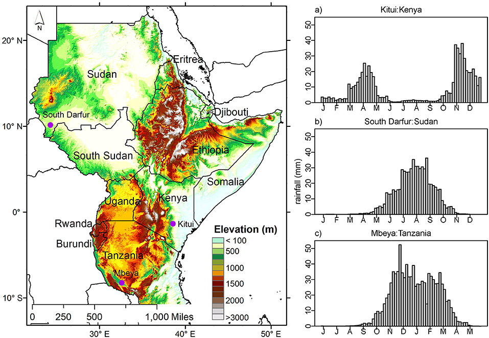
Figure 1. Geographical location of East Africa and average (2000–2018) rainfall over three level 1 administrative districts, (A) Kitui in Kenya, (B) South Darfur in Sudan, and (C) Mbeya in Tanzania. Rainfall source: Climate Hazards Infrared Precipitation with Stations.

NDVI and ET From Remote Sensing Measurements

Since 2003, NDVI and actual ET data have been produced by the U.S. Geological Survey (USGS) Famine Early Warning Systems Network (FEWS NET) using the operational simplified surface energy balance (SSEBop) model (Senay et al., 2013). SSEBop is one of many energy balance–based approaches for estimating ET using remote sensing measurements. The SSEBop setup is based on the Simplified Surface Energy Balance (SSEB) approach (Senay et al., 2013) with a unique parameterization for operational applications. It combines ET fractions generated from remotely sensed MODIS thermal imagery, acquired every 10 days at 1 × 1 km spatial resolution, with reference ET using a thermal index approach. The unique feature of the SSEBop parameterization is that it uses pre-defined, seasonally dynamic, boundary conditions that are unique to each pixel for the “hot/dry” and “cold/wet” reference points (FEWSNET, 2019). The original formulation of SSEB is based on the hot and cold pixel principles of SEBAL (Bastiaanssen et al., 1998) and METRIC (Allen et al., 2007) models. While there are many NDVI and ET products from remote sensing measurements available, the use of MODIS NDVI (Jenkerson et al., 2010) and SSEBop ET in this research is primarily determined by the consistency in their method and production and their long history of readily available data. Furthermore, SSEBop ET estimates were found to be in good agreement with observed FLUXNET ET (Velpuri et al., 2013).

ET From Land Surface Models

Utilizing NASA's state-of-the-art Land Information System (LIS) (Kumar et al., 2008) framework, FEWS NET Land Data Assimilation System (FLDAS) incorporates multiple LSM and produces multi-forcing estimates of land surface states and fluxes such as ET and soil moisture. The output variables are driven by the CHIRPS rainfall product that performs well over data sparse regions. CHIRPS is available over a long historical record, and complements other remote sensing products used by FEWS NET for vegetation, drought, and food security monitoring (McNally et al., 2017). We included ET from three LSMs to better understand their usefulness in monitoring vegetation and drought over East Africa. The ET from the LSMs used in this study include Noah, Variable Infiltration Capacity (VIC), and Catchment Land Surface Model (CLSM). The meteorological forcing data for the LSMs come from NASA's Modern Era Reanalysis for Research and Applications, version 2 (MERRA 2) (Bosilovich et al., 2015). Other parameters include GTOPO 30 elevation, MODIS International Global Biosphere Project (IGBP) land cover for Noah, University of Maryland (UMD) land cover for VIC (Hansen et al., 2000; Friedl et al., 2010), National Centers for Environmental Prediction (NCEP) monthly greenness fraction, albedo (Gutman and Ignatov, 1998; Csiszar and Gutman, 1999), and STATSGO/FAO soil texture. These LSMs use monthly climatology of greenness fraction or leaf area index (LAI) derived from composites of NDVI dataset (Myneni et al., 1997; Gutman and Ignatov, 1998; Dirmeyer et al., 2006) to parameterize vegetation presence. They do not require time series of vegetation information (e.g., NDVI, LAI).

Noah

The Noah LSM (Chen et al., 1996) employs a single column soil-vegetation-atmosphere transfer scheme, discretized using finite difference methods and split-hybrid (water and energy balance) temporal integration. We adopted model version 3.3, which runs at a 15-min timestep and produces ET at 0.1° spatial and daily temporal resolutions. ET in Noah 3.3 includes three components: wet canopy evaporation, transpiration, and evaporation from bare soil. The transpiration is defined using Penman-Monteith formulation with stomatal resistance and constrains using water storage terms that are dependent upon precipitation instead of vapor pressure. The bare soil evaporation is parametrized with soil moisture and the wet canopy evaporation and transpiration are functions of the intercepted canopy water content, which is a residual of water balance. ET is the sum of these three components.

VIC

The VIC model is a semi-distributed macroscale hydrologic model (Liang et al., 1994) in which ET includes similar components as in Noah. The computation of wet canopy evaporation and transpiration is similar to Noah, but unlike Noah the maximum intercepted canopy water content is a function of LAI climatology in VIC. The soil component of VIC employs an area integration to define the soil moisture constraint on transpiration defined using Penman-Monteith with zero stomatal resistance. VIC runs at a 1-h timestep in energy and water balance mode and produces ET at 0.25° spatial resolution.

CLSM

CLSM (Koster et al., 2000) was developed by the NASA Global Modeling and Assimilation Office and is the land-surface component of the Goddard Earth Observing System model version 5 general circulation model. It simulates water and energy balances on irregular topographically derived catchments. ET is calculated from three water balance prognostic variables, surface excess, root zone excess, and catchment deficit, for the dynamically changing saturated, non-saturated, and below wilting areas within the catchment. The primary soil moisture prognostic variable is the catchment deficit, defined as the average amount of water that would have to be added to bring the catchment to saturation. The root zone excess and surface excess describe average amounts of water that are out of equilibrium within the root zone and surface across the catchment. CLSM runs at a 15-min timestep and produces ET at 0.1° spatial and daily temporal resolutions.

Data Processing

Prior to performing the analyses, all the data were collocated in both space and time. The spatial resolution of LSM ET is 0.1°, SSEBop is 1 km, and NDVI is 250 m. Therefore, all the datasets were resampled to 5 km spatial resolution. The three datasets are also available at different temporal scales; LSM ET is daily, NDVI is a 10-days composite, and SSEBop ET is dekadal (10-days equivalent), thus all the respective datasets were temporally aggregated to a monthly timescale. Additionally, the NDVI time series was smoothed using the weighted least-squares approach to remove artifacts caused by unexpected distortions (e.g., clouds, missing data). Prior to the computation, we masked out the areas that receive <200 mm of rainfall annually as desert regions of East Africa (Nicholson, 1996). Studies show anomalies rather than actual values are better indicators for vegetation conditions (Tadesse et al., 2015), therefore, we used anomalies in the analyses. ET anomalies for any given 10-days period were calculated by subtracting the 10-days period value from its historical median (2003–2016). Similarly, NDVI anomalies were calculated by subtracting the 10-days value from its historical median (2003–2016). After computing the mean μ and standard deviation σ, the LSM ET and NDVI anomalies were linearly scaled to the data space of SSEBop ET using Equations (1, 2). We also standardized anomalies for ET and NDVI to bring them under the same scale. These composites allow qualitative comparison of how similarly each of the datasets represents vegetation conditions for different hydrologic regimes over the study area. However, they do not provide direct information with respect to interannual comparisons between the datasets.

$\begin{array}{ll}{E^{\prime }}_{LSM}={\mu }_{SSEBop}+(E_{LSM}-{\mu }_{LSM})\frac{{\sigma }_{SSEBop}}{{\sigma }_{LSM}}& (1)\end{array}$

$\begin{array}{ll}{E^{\prime }}_{NDVI}={\mu }_{SSEBop}+(E_{NDVI}-{\mu }_{NDVI})\frac{{\sigma }_{SSEBop}}{{\sigma }_{NDVI}}& (2)\end{array}$

where E and E′ are the actual and scaled anomalies.

The annual maximum vegetation fraction derived from 12 years of Collection 5 MODIS NDVI data (MOD13A2) (Broxton et al., 2014) and IGBP land cover map were processed to use them in the relationship and error analyses between ET and NDVI by vegetation fractions and land cover types. The descriptions of the IGBP land cover classes are provided in Table 1.

TABLE 1

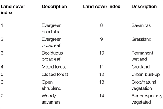
Table 1. International Geosphere Biosphere Program (IGBP) land cover classes.

Triple Collocation Analysis

Triple Collocation (TC) (Stoffelen, 1998) is a statistical method for characterizing consensus and discrepancies across multiple independent datasets. TC analysis has been used to estimate the random errors in NDVI and ET variables. TC analysis is particularly valuable in regions that lack in situ observations for evaluations, as consensus anomaly estimates derived from multiple independent datasets can be interpreted as a measure of confidence in the absence of adequate in situ evaluation data (van der Schalie et al., 2018). TC uses a set of three or more linearly related and collocated variables with independent error structures. It produces root mean square error (RMSE) of the random error component of the individual variable, in the absence of a variable that can be used as the absolute truth (van der Schalie et al., 2018). We employed TC analysis to quantify random errors in LSM ET, SSEBop ET, and NDVI where two of the variables were measuring hydrologic flux and the third one was measuring vegetation vigor. The variables depict reasonable cross-correlations across most of the study area, indicating linear relationships between them at monthly scale. Therefore, they are suitable for TC analysis framework. As stated before, the objective is not to validate any one variable against a different one, but rather to evaluate the skill of these products relative to one another and how the variables can be used together in optimizing vegetation monitoring in East Africa. The TC analysis is performed with the assumption that errors in the datasets are uncorrelated between each other and are independent (Gruber et al., 2016). The LSMs are forced with CHIRPS and MERRA2 inputs, whereas the primary forcing for SSEBop is MODIS radiometric temperature data, and NDVI is derived from MODIS surface reflectance data. In addition, there are substantial differences in underlying modeling approaches between LSM ET and SSEBop ET. Therefore, it is fair to assume that errors in these datasets are independent and uncorrelated.

In this study, we have taken an ensemble mean of the Noah, VIC, and CLSM ET anomaly time series because of the similarities between them and designated the ensemble mean as “LSM ET” in successive analyses. Table 2 shows the correlations between Noah, VIC, and CLSM ET by country. As required, we designated SSEBop ET as the reference variable, which by no means assumes that the SSEBop is perfect, but rather we assume errors in the SSEBop ET are effectively independent from those impacting errors in LSM ET and NDVI. Finally, the TC errors were computed for the May–October and November–April composites for each of the datasets, using the following equations:

$\begin{array}{ll}{\epsilon }_{LSM}=\langle (E_{LSM}^{\prime }-E_{SSEBop})(E_{LSM}^{\prime }-E_{NDVI}^{\prime })\rangle & (3)\end{array}$

$\begin{array}{ll}{\epsilon }_{NDVI}=\langle (E_{NDVI}^{\prime }-E_{SSEBop})(E_{NDVI}^{\prime }-E_{LSM}^{\prime })\rangle & (4)\end{array}$

$\begin{array}{ll}{\epsilon }_{SSEBop}=\langle (E_{SSEBop}-E_{LSM}^{\prime })(E_{SSEBop}-E_{NDVI}^{\prime })\rangle & (5)\end{array}$

where ε is the TC error for each dataset, E and E′ are the actual data scaled data, respectively, and 〈−〉 is the corresponding average over the period. TC produces the random error metric, where numbers closer to zero indicate better performance and vice versa.

TABLE 2

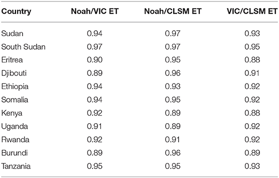
Table 2. Average correlation coefficient by country for between Noah, VIC, and CLSM ET.

Statistical Measure

Spatially distributed statistical measures, including long-term annual mean, standardized monthly anomalies (spatial, temporal), and Pearson's correlation coefficient r, are used to compare these variables during the wetter half of the year.

$\begin{array}{ll}r=\frac{{\displaystyle {\sum }_i^n}(E_i-\overline{E})(S_i-\overline{S})}{\sqrt{{\displaystyle {\sum }_i^n}{(E_i-\overline{E})}^2{\displaystyle {\sum }_i^n}{(S_i-\overline{S})}^2}},-1\le r\le 1& (6)\end{array}$

where E_i represents the LSM ET or NDVI monthly anomaly, S_i represents monthly SSEBop ET anomaly, $\overline{E}$ and $\overline{S}$are the respective mean, n is the total number of data records in the time series, and the subscript i denotes the ith number of samples. As suggested in Hain et al. (2011), we used anomalies instead of actual values for correlation to minimize impacts of differences in mean and standard deviation values between SSEBop ET, LSM ET, and NDVI variables due to differences in input data and modeling approaches.

Results

Annual ET

The annual total ET (in mm) that reflects the period 2003–2016 is shown in Figure 2 for the LSMs and for SSEBop ET. The annual total ET values over the land surface (top row in Figure 2) are generally highest across the Inter-Tropical Convergence Zone (ITCZ) and over the Ethiopian Highlands. In contrast, low ET can be seen over Somalia. The spatial distribution of annual ET resembles the annual rainfall gradient in the region, which is mostly determined by surface heating and confluence of the tropical easterlies (Novella and Thiaw, 2013). A CHIRPS-based rainfall gradient map over East Africa is available in Figure 2A of Fenta et al. (2017).

FIGURE 2

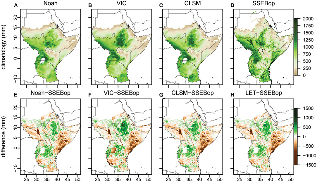
Figure 2. Annual total evapotranspiration (ET; in mm) for the period 2003–2016 from (A) Noah, (B) VIC, (C) CLSM, (D) SSEBop. The bottom row shows the difference in ET climatology between (E) Noah minus SSEBop, (F) VIC minus SSEBop, (G) CLSM minus SSEBop, and (H) ensemble mean of Noah, VIC, and CLSM minus SSEBop.

Over the region, high annual ET values of over 1,400 mm are found in the southern part of the Ethiopian Highlands. High ET of around 1,000 mm per year is also found in southwestern South Sudan and adjacent areas of Lake Victoria in Uganda and Kenya. Besides the desert areas, parts of southern Sudan, the leeward side of the Ethiopian Highlands, eastern Somalia, and Kenya produce ET below 200 mm per year. The spatial distributions of annual total ET for the three models are similar. The correlation coefficient between Noah, VIC, and CLSM ET are greater than 0.8 with P < 0.1 across the study area. At country level, the average correlation coefficient is even greater (Table 2) between these LSM ET. The similar spatial resemblance of Noah, VIC, and CLSM ET further justifies use of their ensemble mean. A difference map between the LSM ensemble mean ET and SSEBop ET is shown in Figure 2H along with differences between SSEBop ET and individual LSM (Noah, VIC, CLSM) ET in Figures 2E–G.

Spatial Anomaly Comparison

Bearing in mind the predominantly arid conditions of the study region, we evaluated the performances of these variables in identifying vegetation conditions during different hydrologic regimes. To do so, we mapped the standardized seasonal anomaly composites of ET and NDVI over the wetter half of the year for the last 12 years from the time series (2004/05 to 2015/16). We used standardized anomalies because of the differences in units for ET and NDVI. The seasonal anomaly maps are presented in Figure 3 for the 2004/2005 to 2009/2010 seasons and in Figure 4 for the 2010/2011 to 2015/2016 seasons. The seasonal anomalies were computed over May to October over Sudan, South Sudan, Ethiopia, Eritrea, Djibouti, and Somalia; and over November to April over Kenya, Uganda, Rwanda, Burundi, and Tanzania.

FIGURE 3

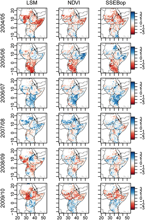
Figure 3. Standardized anomaly composites of LSM ET, NDVI, and SSEBop ET over the wetter half of the year for the period 2004–2010. May–October for Sudan, South Sudan, Ethiopia, Eritrea, Djibouti, Uganda, and Somalia, and November–April for Kenya, Uganda, Rwanda, Burundi, and Tanzania.

FIGURE 4

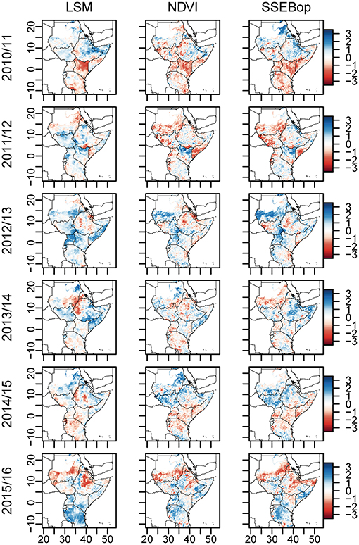
Figure 4. Standardized anomaly composites of LSM ET, NDVI, and SSEBop ET over the wetter half of the year for the period 2011–2016. May–October for Sudan, South Sudan, Ethiopia, Eritrea, Djibouti, and Somalia, and November–April for Kenya, Uganda, Rwanda, Burundi, and Tanzania.

The droughts of 2004/2005 and 2009/2010 due to failed rainfall (McNally et al., 2016) have been well-captured in LSM ET, SSEBop ET, and NDVI. The extreme severity of the 2004 drought over eastern Ethiopia, Somalia and the 2009/2010 drought over South Sudan have been particularly well-depicted by LSM ET (Gebremeskel et al., 2019), while the 2010/2011 drought over Somalia and Kenya (Robinson et al., 2019) has been well-portrayed by all three variables. Conversely, healthy to average vegetation condition of 2006/2007 due to the wettest rainfall season since 1982 across the region has been better reflected in all three variables.

More recently, the 2015/2016 El Niño caused a dramatic decrease in rainfall, especially over Ethiopia and Sudan, resulting in severe drought (Qu et al., 2019), which has been well-identified in LSM ET. While a coherent condition is portrayed by LSM ET, NDVI, and SSEBop ET during the anomalously dry or wet years, they tend to differ slightly during some hydrologically average years. For example, during 2008/2009 LSM ET differs from NDVI and SSEBop ET over South Sudan by showing below average conditions, and in 2011/2012 LSM ET shows above average conditions over the same area while NDVI and SSEBop ET show below average conditions.

Temporal Anomaly Correlation

Figure 5 shows the temporal cross-correlation between the anomalies of the variables (between LSM ET and SSEBop ET in Figure 5A, between LSM ET and NDVI in Figure 5B, and between SSEBop and NDVI in Figure 5C) using monthly composites during the wetter half of the year for the period 2003–2016. This provides information about the temporal correlation between two datasets and yields a measure of skill for either LSM ET, SSEBop, or NDVI relative to each other. Only the pixels that have a statistically significant correlation coefficient at 90% confidence interval (P < 0.1) are shown on the maps in Figure 5. In general, LSM shows good temporal agreement with SSEBop or NDVI over Ethiopian Highlands, Kenya, Uganda, and central Tanzania, but poor performance over South Sudan and southern Somalia. In contrast, SSEBop ET is strongly correlated with NDVI across much of the area. LSM exhibits statistically significant r values over 67% of the pixels, while NDVI shows statistically significant correlation over 77% of the pixels with SSEBop. LSM also exhibits statistically significant correlation with NDVI over 72% of the pixels. Although SSEBop shows better correlation with NDVI than LSM ET, portions of the study area are associated with statistically significant negative correlation between SSEBop and NDVI. These results relate with findings of Joiner et al. (2018) based on weekly climatology composites of fraction of potential ET and NDVI over East Africa. The same study also suggests up to 2 weeks of time lag in NDVI response. However, we have observed, when NDVI is summarized to monthly scale, the lag becomes less evident for the relationships between NDVI and ET over East Africa.

FIGURE 5

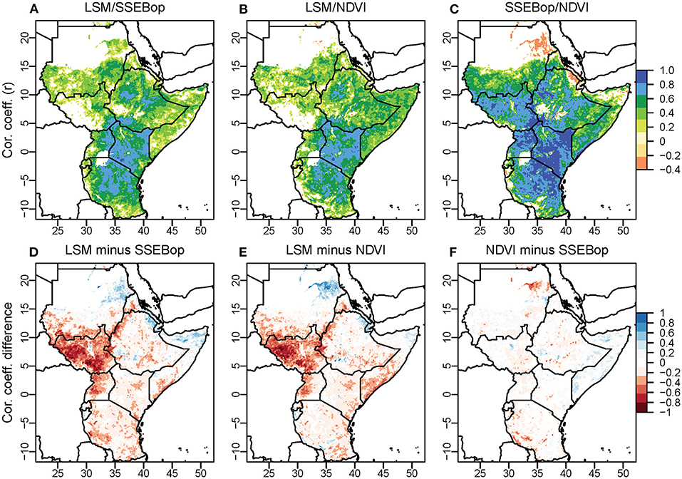
Figure 5. Time series anomaly cross-correlation coefficient calculated over the wetter half of the year for 2003–2016 for (A) LSM ET/SSEBop ET, (B) LSM ET/NDVI, and (C) SSEBop ET/NDVI. (D) The difference in anomaly cross-correlation where blue (red) shading indicates LSM ET/NDVI correlation is greater (less) than NDVI/SSEBop ET correlation. (E) The difference in anomaly cross-correlation where blue (red) shading indicates LSM ET/SSEBop ET correlation is greater (less) than NDVI/SSEBop ET correlation. Only pixels that exhibit a statistically significant correlation at 90% confidence interval are shown (p < 0.1). (F) The difference in anomaly cross-correlation where blue (red) shading indicates LSM ET/SSEBop ET correlation is greater (less) than LSM ET/NDVI correlation.

Figures 5D–F shows differences in temporal cross-correlation between the variables, comparing correlation computed between them. Figure 5D shows the difference in correlation between LSM/NDVI and SSEBop/NDVI. Blue shading denotes pixels where LSM is more strongly correlated and red shading denotes pixels where SSEBop is more strongly correlated with NDVI, highlighting regions where each variable shows relative advantages and disadvantages. Similarly, in Figure 5E, blue shading shows pixels where LSM ET is more strongly correlated with SSEBop ET and red shading indicates pixels where NDVI is more strongly correlated with SSEBop ET. It can be inferred that LSM ET is not a good indicator of vegetation conditions over South Sudan.

TC Analysis

The spatial distributions of relative error estimates computed using Equations (3–5) for LSM ET, NDVI, and SSEBop ET are shown in Figure 6. The TC error values are relative to SSEBop ET and are shown in millimeters as the LSM ET and NDVI have been linearly scaled to SSEBop ET as required by the TC computation. The domain-averaged relative TC errors are observed to be 130 mm for the LSM ET and 93 mm for SSEBop ET.

FIGURE 6

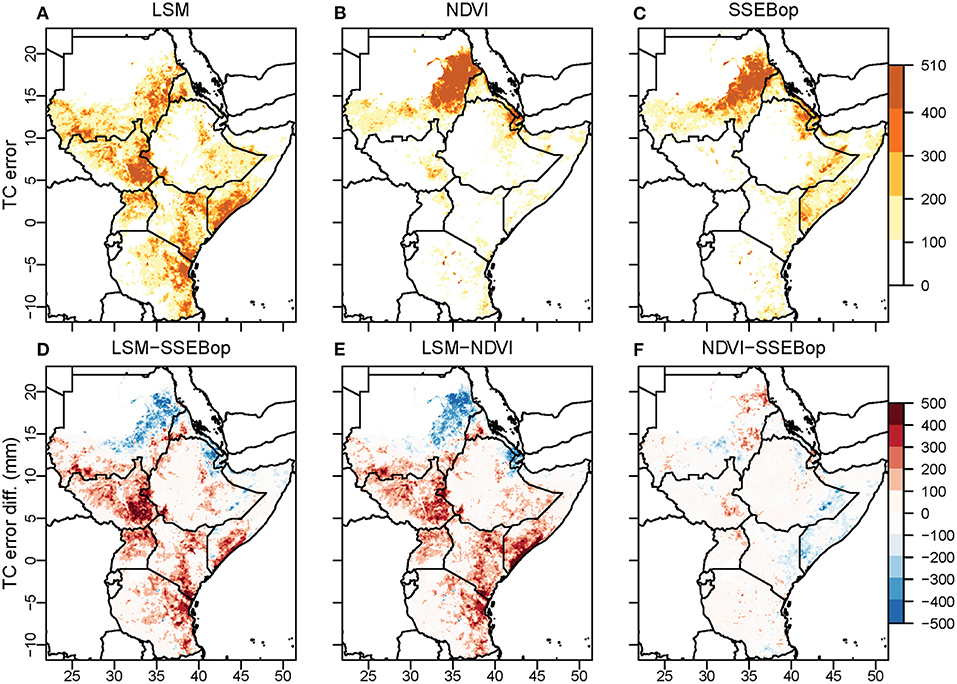
Figure 6. Triple Collocation (TC) error estimates (in mm) over the 2003–2016 for (A) LSM ET, (B) NDVI, and (C) SSEBop ET. LSM ET and NDVI have been rescaled to SSEBop ET. The difference in TC error between (D) LSM ET and SSEBop ET, (E) LSM ET and NDVI, (F) SSEBop ET and NDVI.

Although the domain-averaged TC errors are relatively low, there are substantial differences in spatial distribution of the errors within the study area. LSM ET shows high TC error over South Sudan, southern Somalia, and eastern Tanzania; NDVI shows high TC error over eastern Sudan; and SSEBop shows high TC error over eastern Sudan and the border region between Kenya and Somalia. Figures 6D–F shows the difference in TC errors between LSM, NDVI, and SSEBop to highlight areas of high and low TC errors by each variable. The red shaded pixels in Figures 6D,E denote where LSM has higher TC error and the blue shaded pixels where LSM has lower TC errors compared to TC errors in SSEBop and NDVI. It also becomes clear that the areas of positive LSM TC errors are similar to the areas where LSM did not correlate well with SSEBop or NDVI and vice versa (Figures 5D,E). These similarities indicate that both TC error and cross-correlation techniques are providing qualitatively similar information. Similar findings are also reported by Hain et al. (2011) while comparing three different soil moisture datasets in the U.S.

Discussion

Both LSM ET and SSEBop ET show similar spatial patterns in annual total ET distribution but are not identical in magnitude. The high LSM or SSEBop ET along the ITCZ and Ethiopian Highlands can be attributed to the intense surface heating and high precipitation amounts over the Ethiopian Highlands. All the models agree well with very low ET over the arid regions of eastern Ethiopia and Somalia. Precipitation is very low over these regions because of the cool air ventilated from the western Indian Ocean where sea surface temperatures are low along with cool ocean currents adjacent to the East Africa land area (Yang et al., 2015), rendering as poor vegetative growth. ET from VIC tends to show higher estimates than SSEBop and the other two models, especially over the Ethiopian Highlands. Over southern Somalia, encompassing the catchments of the Juba and Shabelle Rivers and central South Sudan, all the LSMs tend to underestimate ET. SSEBop ET obtains its measurement based on radiometric temperature differences between theoretical hot and cold pixels. The radiometric temperatures vary depending on the amount of vegetation present. Typically, the higher the vegetation presence, the lower the surface temperature over well-watered locations because of the cooling effect of ET. Therefore, the performance in ET computation is expected to increase with increasing vegetation cover as the processes integrate both the effects of surface evaporation and plant transpiration. Thus, SSEBop ET could be more responsive to changes in the presence of vegetation cover than the LSM ET. The spatial resolution difference between LSM ET and SSEBop ET could also have played a role in resolving energy balance while estimating ET.

It can be inferred from Figures 3, 4 that ET from both LSM and remote sensing measurements could be better indicators of vegetation conditions during extreme drought events (e.g., in the years 2004/2005, 2009/2010, and the El Niño year of 2015/2016). Because they are mostly driven by surface energy balance, they are more sensitive to higher atmospheric demand due to higher temperatures and lower soil moisture, which relates to lack of rainfall during extreme drought events. Conversely, NDVI could be a better indicator of vegetation conditions during wetter than normal conditions because it is more sensitive to availability of water due to higher than normal rainfall conditions (e.g., the year of 2006/2007).

While LSM ET correlates positively with SSEBop ET and NDVI over a majority of the study area, some areas had negative correlation between SSEBop and NDVI. These areas of negative correlation collocate with both dense and sparsely vegetated areas (Figure 5C). This can be attributed to the issues in NDVI due to signal saturation over densely vegetated areas and high noise-to-signal ratio over areas where the presence of vegetation is very low (Huete, 1988). To investigate these further, we plotted the average correlation as a function of vegetation fraction and type in Figures 7, 8, respectively. The cross-correlation does not vary between LSM ET and SSEBop ET with the increase of vegetation presence, but it increases between SSEBop ET and NDVI. This means that SSEBop ET and NDVI are more influenced by vegetation cover than it is for LSM ET (Figure 7B). On the other hand, the correlation between LSM ET and SSEBop ET is better over vegetation fraction <18% (Figure 7C). NDVI suffers from high noise-to-signal ratio over areas with high albedo (low vegetation cover) and SSEBop ET utilizes a correction factor to adjust surface temperature while computing ET fraction over high albedo areas (Senay et al., 2013). The correction process might have helped correlate SSEBop ET better with LSM ET than with NDVI over sparsely vegetated areas. The average correlation by land cover types also confirms that neither SSEBop ET nor NDVI performs well over evergreen and deciduous broadleaf as well as barren/sparsely vegetated land cover types (Figure 8C). This implies that LSM ET could be a better indicator for vegetation condition over sparsely vegetated areas. Over moderately vegetative areas (vegetation fraction of > 20%), a consistent correlation (r > 0.5) can be observed between ET and NDVI at the monthly time scale, which implies that any of these variables could be a good indicator of vegetation condition over moderately vegetated areas. A similar pattern of correlation between ET and NDVI is also reported by Mbatha and Xulu (2018) during 2002–2016 over southern Africa.

FIGURE 7

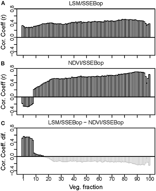
Figure 7. The cross-correlation coefficient for the 2003–2016 as a function of vegetation fraction for (A) LSM ET/SSEBop ET, (B) NDVI/SSEBop ET, and (C) the difference in correlation between LSM ET/SSEBop ET and NDVI/SSEBop ET.

FIGURE 8

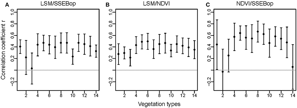
Figure 8. The average correlation for the 2003–2016 by IGBP land cover types for (A) LSM ET/SSEBop ET, (B) LSM ET/NDVI, and (C) NDVI/SSEBop ET.

As with the cross-correlations between the variables, the spatial variability of the random error values during the rainy season for each variable has been evaluated as a function of the vegetation fraction (Figure 9). The plots show that the random errors in LSM ET are lower than the random errors in SSEBop ET over low-density vegetated areas (vegetation fraction of 40% or less). When the vegetation fraction increases, the error in LSM gradually increases, but again decreases for the very high end of the vegetation fraction (95% or more) (Figure 9A). As a remotely sensed surface temperature–based estimation of SSEBop ET, it is expected that the accuracy of the estimate would decrease over areas of dense vegetation mostly due to inaccuracies in remotely sensed surface temperature data over high densely vegetated areas. Compared to NDVI errors, LSM ET errors are lower over the low (20% or lower) end of the vegetation fraction and the errors start to decrease for LSM ET as the vegetation fraction increases toward full coverage (95% or higher). Figure 9C shows that NDVI might have the most error over the low and high ends of the vegetation fraction areas and therefore may not be a good variable for vegetation monitoring over these areas. Over these areas, LSM ET is most likely to provide better information for vegetation monitoring. These results are also consistent with correlation analysis (Figure 7), which indicates that LSM ET shows better correlations compared to other two data sources over the low-density vegetated areas.

FIGURE 9

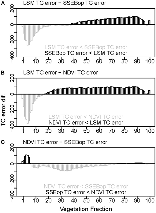
Figure 9. Average TC error difference as a function of vegetation fraction for (A) LSM ET TC error minus SSEBop ET TC error, (B) LSM ET TC error minus NDVI TC error, and (C) NDVI TC error minus SSEBop ET TC error.

To further investigate the random errors by vegetation type, we plotted average TC error for each variable as a function of vegetation type in Figure 10. Only a few pixels belong to evergreen needleleaf forest (type 1), permanent wetland (type 10), and urban built-up (type 12) areas in the study area; therefore, they may not be a true representation of the TC errors. Among other land cover types, LSM ET has lower TC error over cropland and barren/sparsely vegetated areas compared to TC error in SSEBop ET and NDVI. For the remaining land cover types, TC errors in LSM ET are higher than those in SSEBop ET or NDVI. More specifically, LSM ET TC errors are higher over the savanna and woody savanna land cover types collocated in South Sudan. This could be due to vegetation parameterization differences in LSM ET.

FIGURE 10

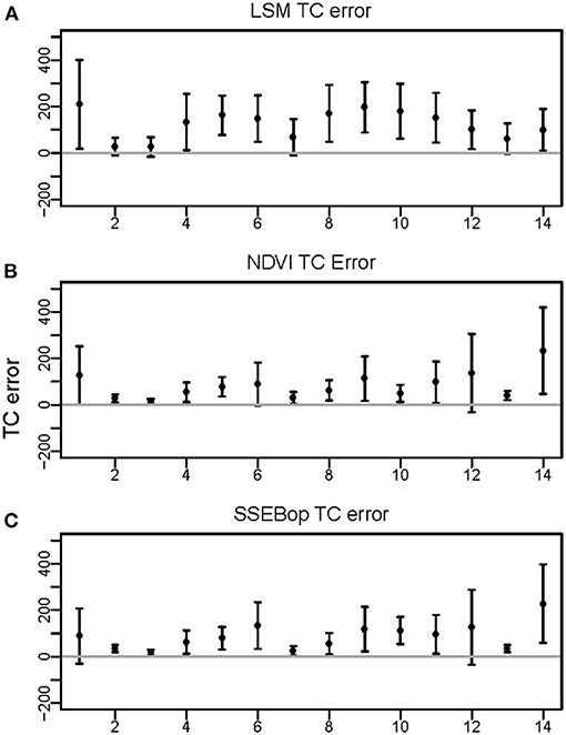
Figure 10. Average TC error by land cover type for (A) LSM ET TC error, (B) NDVI TC error, and (C) SSEBop ET TC error. The corresponding vegetation type for the numbers along the x-axis are shown in Table 1.

Finally, we compiled the TC errors for each pixel to identify the variable with the lowest random error. The map in Figure 11 shows the lowest TC error by variable for each pixel. Based on this map, NDVI would provide better information for vegetation monitoring over 41% of the study area, mostly covering parts of Ethiopia, Somalia, and eastern Kenya. SSEBop would provide better information over 40% of the study area, covering the Ethiopian Highlands, South Sudan, western Kenya, Uganda, and Tanzania, and LSM ET would provide better information for monitoring vegetation condition over 19% of the study area, mostly covering areas in Sudan, parts of Somalia, Eritrea, and Ethiopia. This map can be used as a guide along with other ancillary socio-economic information by analysts to optimize vegetation monitoring using both ET and NDVI for drought and food security assessments.

FIGURE 11

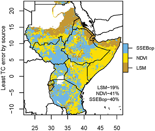
Figure 11. Map of lowest TC error for LSM ET, SSEBop ET, and NDVI for the 2003–2016 period.

Conclusions

We performed cross-correlation and triple collocation analyses to characterize relationships between ET from remotely sensed measurements (SSEBop) and from LSMs (Noah, VIC, and CLSM) and a biophysical variable directly computed from surface reflectance measured by satellite sensors, NDVI. In general, SSEBop ET and LSM ET show good spatial agreement in annual total ET distribution following the annual precipitation gradient in East Africa. However, there are differences in magnitude between them. LSM ET and SSEBop ET were found to be better indicators for vegetation monitoring during the extreme drought events, while NDVI could provide better information for vegetation conditions during wetter than normal conditions. Spatially, LSM ET correlates reasonably well with NDVI and SSEBop ET over most of the study area except over South Sudan and southern Somalia, whereas SSEBop ET and NDVI show relatively better agreement over southern Somalia. Correlations between the variables suggest that LSM ET could be a better indicator for vegetation condition over sparsely vegetated areas, while any of these variables could be a good indicator of vegetation condition over moderately vegetated areas. The TC error estimation technique estimated relative random error in LSM ET, SSEBop ET, and NDVI. The errors of these variables suggest that NDVI might have the most error over the low and high ends of the vegetation fraction areas and therefore may not be a good variable for vegetation monitoring over these areas. Over these areas, LSM ET is most likely to provide important information for vegetation monitoring. Finally, a map was produced by compiling the lowest random error by variable that can be used in optimizing vegetation monitoring by using LSM ET, SSEBop ET, and NDVI over the areas where they perform the best. The map would be useful especially over the extremely dry landscapes of Djibouti and parts of arid and semi-arid lands of Somalia, Ethiopia, and northern and eastern Kenya where very high reflectance of sandy soils poses critical challenges in comprehensive monitoring of vegetation conditions. As NDVI emphasizes vegetation conditions from water supply perspective and ET emphasizes vegetation conditions from water demand, perhaps a ratio of NDVI and ET could also be explored for comprehensive vegetation monitoring. While this study provides a framework for optimizing vegetation monitoring for drought and food security assessments over East Africa, the framework can be adopted to optimize vegetation monitoring over any other drought and food insecure regions of the world.

Data Availability Statement

Publicly available datasets were analyzed in this study. This data can be found at: https://earlywarning.usgs.gov; http://disc.sci.gsfc.nasa.gov/uui/datasets?keywords=FLDAS; https://earthdata.nasa.gov/search?q=igbp+land+cover.

Author Contributions

SP and AM conceptualized the research. SP defined the methods, analyzed the findings, composed the figures, and drafted the manuscript. KA drafted and provided CLSM data. AM, KA, and MB provided additional analysis. All authors revised and improved the manuscript.

Funding

This research was supported by the U.S. Agency for International Development (USAID) Famine Early Warning Systems Network Interagency agreement with the U.S. Geological Survey, USAID Interagency Agreement with NASA Goddard and NASA Harvest.

Conflict of Interest

AM and KA were employed by the company, Science Application International Corporation.

The remaining authors declare that the research was conducted in the absence of any commercial or financial relationships that could be construed as a potential conflict of interest.

Acknowledgments

Work performed under USGS contract 140G0119C0001.We sincerely thank Dr. Gabriel Senay and Stefanie Kagone for providing SSEBop ET data and suggestions made throughout the research. We greatly appreciate the astute comments made by the reviewers and technical comments and edits provided by USGS reviewers that helped us to improve the manuscript. Any use of trade, firm, or product names is for descriptive purposes only and does not imply endorsement by the U.S. Government. All the data sources used in this study are publicly available with links in the cited references respectively.

References

Alemu, H., Senay, G. B., Kaptue, A. T., and Kovalskyy, V. (2014). Evapotranspiration variability and its association with vegetation dynamics in the Nile Basin, 2002–2011. Remote Sensing 6, 5885–5908. doi: 10.3390/rs6075885

CrossRef Full Text | Google Scholar

Allen, R. G., Tasumi, M., and Trezza, R. (2007). Satellite-based energy balance for mapping evapotranspiration with internalized calibration (METRIC)—model. J. Irrigat. Drainage Eng. 133, 380–394. doi: 10.1061/(ASCE)0733-9437(2007)133:4(380)

CrossRef Full Text | Google Scholar

Anyamba, A., and Tucker, C. J. (2005). Analysis of Sahelian vegetation dynamics using NOAA-AVHRR NDVI data from 1981–2003. J. Arid Environ. 63, 596–614. doi: 10.1016/j.jaridenv.2005.03.007

CrossRef Full Text | Google Scholar

Baruga, C. K., Kim, D., and Choi, M. (2019). A national-scale drought assessment in Uganda based on evapotranspiration deficits from the Bouchet hypothesis. J. Hydrol. 580:124348. doi: 10.1016/j.jhydrol.2019.124348

CrossRef Full Text | Google Scholar

Bastiaanssen, W., Noordman, E., Pelgrum, H., Davids, G., Thoreson, B., and Allen, R. (2005). SEBAL model with remotely sensed data to improve water-resources management under actual field conditions. J. Irrigat. Drainage Eng. 131, 85–93. doi: 10.1061/(ASCE)0733-9437(2005)131:1(85)

CrossRef Full Text | Google Scholar

Bastiaanssen, W. G., Menenti, M., Feddes, R., and Holtslag, A. (1998). A remote sensing surface energy balance algorithm for land (SEBAL). 1. Formulation. J. Hydrol. 212, 198–212. doi: 10.1016/S0022-1694(98)00253-4

CrossRef Full Text | Google Scholar

Biggs, T., Petropoulos, G., Velpuri, N., Marshall, M. H., Glenn, E., Nagler, P., et al. (2015). “Remote sensing of actual evapotranspiration from croplands,” in Remote Sensing of Water Resources, Disasters, and Urban Studies, ed P. S. Thenkabail (Boca Raton, FL: Taylor & Francis), 59–100.

Google Scholar

Bosilovich, M. G., Akella, S., Coy, L., Cullather, R., Draper, C., Gelaro, R., et al (2015). MERRA-2: Initial Evaluation of the Climate. Vol. 43. NASA Technical Report. Series on Global Modeling and Data Assimilation, NASA/TM–2015-104606. Available online at: https://gmao.gsfc.nasa.gov/pubs/docs/Bosilovich803.pdf (accessed November 10, 2019).

Google Scholar

Brown, M. E. (2016). Remote sensing technology and land use analysis in food security assessment. J. Land Use Sci. 11, 623–641. doi: 10.1080/1747423X.2016.1195455

CrossRef Full Text | Google Scholar

Broxton, P. D., Zeng, X., Scheftic, W., and Troch, P. A. (2014). A MODIS-based global 1-km maximum green vegetation fraction data set. J. Appl. Meteorol. Climatol. 53, 1996–2004. doi: 10.1175/JAMC-D-13-0356.1

CrossRef Full Text | Google Scholar

Chen, F., Mitchell, K., Schaake, J., Xue, Y., Pan, H. L., Koren, V., et al. (1996). Modeling of land surface evaporation by four schemes and comparison with FIFE observations. J. Geophys. Res. Atmos. 101, 7251–7268. doi: 10.1029/95JD02165

CrossRef Full Text | Google Scholar

Chirouze, J., Boulet, G., Jarlan, L., Fieuzal, R., Rodriguez, J., Ezzahar, J., et al. (2013). Inter-comparison of four remote sensing based surface energy balance methods to retrieve surface evapotranspiration and water stress of irrigated fields in semi-arid climate. Hydrol. Earth Syst. Sci. Disc. 18, 1165–1188. doi: 10.5194/hessd-10-895-2013

CrossRef Full Text | Google Scholar

Csiszar, I., and Gutman, G. (1999). Mapping global land surface albedo from NOAA AVHRR. J. Geophys. Res. Atmos. 104, 6215–6228. doi: 10.1029/1998JD200090

CrossRef Full Text | Google Scholar

Dinku, T., Ceccato, P., and Connor, S. J. (2011). Challenges of satellite rainfall estimation over mountainous and arid parts of east Africa. Int. J. Remote Sensing 32, 5965–5979. doi: 10.1080/01431161.2010.499381

CrossRef Full Text | Google Scholar

Dirmeyer, P. A., Gao, X., Zhao, M., Guo, Z., Oki, T., and Hanasaki, N. (2006). GSWP-2: Multimodel analysis and implications for our perception of the land surface. Bullet. Am. Meteorol. Soc. 87, 1381–1398. doi: 10.1175/BAMS-87-10-1381

CrossRef Full Text | Google Scholar

Du, L., Tian, Q., Yu, T., Meng, Q., Jancso, T., Udvardy, P., et al. (2013). A comprehensive drought monitoring method integrating MODIS and TRMM data. Int. J. Appl. Earth Observ. Geoinform. 23, 245–253. doi: 10.1016/j.jag.2012.09.010

CrossRef Full Text | Google Scholar

Fenta, A. A., Yasuda, H., Shimizu, K., Haregeweyn, N., Kawai, T., Sultan, D., et al. (2017). Spatial distribution and temporal trends of rainfall and erosivity in the Eastern Africa region. Hydrol. Process. 31, 4555–4567. doi: 10.1002/hyp.11378

CrossRef Full Text | Google Scholar

FEWSNET (2019). Famine Early Warning Systems Network. FEWS NET. Available online at: https://earlywarning.usgs.gov/fews/product/134 (accessed June 6, 2019).

Google Scholar

Fisher, J. B., Tu, K. P., and Baldocchi, D. D. (2008). Global estimates of the land–atmosphere water flux based on monthly AVHRR and ISLSCP-II data, validated at 16 FLUXNET sites. Remote Sensing Environ. 112, 901–919. doi: 10.1016/j.rse.2007.06.025

CrossRef Full Text | Google Scholar

Friedl, M. A., Sulla-Menashe, D., Tan, B., Schneider, A., Ramankutty, N., Sibley, A., et al. (2010). MODIS Collection 5 global land cover: algorithm refinements and characterization of new data sets. Remote Sensing Environ. 114, 168–182. doi: 10.1016/j.rse.2009.08.016

CrossRef Full Text | Google Scholar

Funk, C., Peterson, P., Landsfeld, M., Pedreros, D., Verdin, J., Shukla, S., et al. (2015). The climate hazards infrared precipitation with stations—a new environmental record for monitoring extremes. Sci. Data 2:150066. doi: 10.1038/sdata.2015.66

PubMed Abstract | CrossRef Full Text | Google Scholar

Funk, C., Shukla, S., Thiaw, W. M., Rowland, J., Hoell, A., McNally, A., et al. (2019). Recognizing the Famine Early Warning Systems Network (FEWS NET): over 30 years of drought early warning science advances and partnerships promoting global food security. Bullet. Am. Meteorol. Soc. 100, 1011–1027. doi: 10.1175/BAMS-D-17-0233.1

CrossRef Full Text | Google Scholar

Gebremeskel, G., Tang, Q., Sun, S., Huang, Z., Zhang, X., and Liu, X. (2019). Droughts in East Africa: causes, impacts and resilience. Earth Sci. Rev. 193, 146–161. doi: 10.1016/j.earscirev.2019.04.015

CrossRef Full Text | Google Scholar

Glenn, E. P., Huete, A. R., Nagler, P. L., Hirschboeck, K. K., and Brown, P. (2007). Integrating remote sensing and ground methods to estimate evapotranspiration. Crit. Rev. Plant Sci. 26, 139–168. doi: 10.1080/07352680701402503

CrossRef Full Text | Google Scholar

Gruber, A., Su, C.-H., Zwieback, S., Crow, W., Dorigo, W., and Wagner, W. (2016). Recent advances in (soil moisture) triple collocation analysis. Int. J. Appl. Earth Observ. Geoinform. 45, 200–211. doi: 10.1016/j.jag.2015.09.002

CrossRef Full Text | Google Scholar

Gutman, G., and Ignatov, A. (1998). The derivation of the green vegetation fraction from NOAA/AVHRR data for use in numerical weather prediction models. Int. J. Remote Sensing 19, 1533–1543. doi: 10.1080/014311698215333

CrossRef Full Text | Google Scholar

Hain, C. R., Crow, W. T., Mecikalski, J. R., Anderson, M. C., and Holmes, T. (2011). An intercomparison of available soil moisture estimates from thermal infrared and passive microwave remote sensing and land surface modeling. J. Geophys. Res. Atmos. 116:JD015633. doi: 10.1029/2011JD015633

CrossRef Full Text | Google Scholar

Hansen, M., DeFries, R., Townshend, J. R., and Sohlberg, R. (2000). Global land cover classification at 1 km spatial resolution using a classification tree approach. Int. J. Remote Sensing 21, 1331–1364. doi: 10.1080/014311600210209

CrossRef Full Text | Google Scholar

Huete, A. R. (1988). A soil-adjusted vegetation index (SAVI). Remote Sensing Environ. 25, 295–309. doi: 10.1016/0034-4257(88)90106-X

CrossRef Full Text | Google Scholar

IGAD (2020). About the Agriculture and Environment Devision. Intergovermental Authority for Development. Available online at: https://igad.int/about-igad/49-about-us/95-about-the-agriculture-and-environment-devision (accessed June 15, 2020).

Google Scholar

Jenkerson, C. B., Maiersperger, T., and Schmidt, G. (2010). eMODIS: A user-friendly data source: U.S. Geological Survey Open-File Report 2010–1055. 10 p. doi: 10.3133/ofr20101055

CrossRef Full Text | Google Scholar

Joiner, J., Yoshida, Y., Anderson, M., Holmes, T., Hain, C., Reichle, R., et al. (2018). Global relationships among traditional reflectance vegetation indices (NDVI and NDII), evapotranspiration (ET), and soil moisture variability on weekly timescales. Remote Sensing Environ. 219, 339–352. doi: 10.1016/j.rse.2018.10.020

PubMed Abstract | CrossRef Full Text | Google Scholar

Justice, C., Holben, B., and Gwynne, M. (1986). Monitoring East African vegetation using AVHRR data. Int. J. Remote Sensing 7, 1453–1474. doi: 10.1080/01431168608948948

CrossRef Full Text | Google Scholar

Kalma, J. D., McVicar, T. R., and McCabe, M. F. (2008). Estimating land surface evaporation: a review of methods using remotely sensed surface temperature data. Surveys Geophys. 29, 421–469. doi: 10.1007/s10712-008-9037-z

CrossRef Full Text | Google Scholar

Kimosop, P. (2019). Characterization of drought in the Kerio Valley Basin, Kenya using the Standardized Precipitation Evapotranspiration Index: 1960– 2016. Singapore J. Trop. Geogr. 40, 239–256. doi: 10.1111/sjtg.12270

CrossRef Full Text | Google Scholar

Klisch, A., and Atzberger, C. (2016). Operational drought monitoring in Kenya using MODIS NDVI time series. Remote Sensing 8:267. doi: 10.3390/rs8040267

CrossRef Full Text | Google Scholar

Kogan, F. N. (1995). Application of vegetation index and brightness temperature for drought detection. Adv. Space Res. 15, 91–100. doi: 10.1016/0273-1177(95)00079-T

CrossRef Full Text | Google Scholar

Koster, R. D., Suarez, M. J., Ducharne, A., Stieglitz, M., and Kumar, P. (2000). A catchment-based approach to modeling land surface processes in a general circulation model: 1. Model structure. J. Geophys. Res. Atmos. 105, 24809–24822. doi: 10.1029/2000JD900327

CrossRef Full Text | Google Scholar

Kumar, S. V., Reichle, R. H., Peters-Lidard, C. D., Koster, R. D., Zhan, X., Crow, W. T., et al. (2008). A land surface data assimilation framework using the land information system: description and applications. Adv. Water Resourc. 31, 1419–1432. doi: 10.1016/j.advwatres.2008.01.013

CrossRef Full Text | Google Scholar

Lanning, M., Wang, L., Scanlon, T. M., Vadeboncoeur, M. A., Adams, M. B., Epstein, H. E., et al. (2019). Intensified vegetation water use under acid deposition. Sci. Adv. 5:eaav5168. doi: 10.1126/sciadv.aav5168

PubMed Abstract | CrossRef Full Text | Google Scholar

Liang, X., Lettenmaier, D. P., Wood, E. F., and Burges, S. J. (1994). A simple hydrologically based model of land surface water and energy fluxes for general circulation models. J. Geophys. Res. Atmos. 99, 14415–14428. doi: 10.1029/94JD00483

CrossRef Full Text | Google Scholar

Mbatha, N., and Xulu, S. (2018). Time series analysis of MODIS-derived NDVI for the Hluhluwe-Imfolozi Park, South Africa: impact of recent intense drought. Climate 6:95. doi: 10.3390/cli6040095

CrossRef Full Text | Google Scholar

McNally, A., Arsenault, K., Kumar, S., Shukla, S., Peterson, P., Wang, S., et al. (2017). A land data assimilation system for sub-Saharan Africa food and water security applications. Sci. Data 4:170012. doi: 10.1038/sdata.2017.12

PubMed Abstract | CrossRef Full Text | Google Scholar

McNally, A., Shukla, S., Arsenault, K. R., Wang, S., Peters-Lidard, C. D., and Verdin, J. P. (2016). Evaluating ESA CCI soil moisture in East Africa. Int. J. Appl. Earth Observ. Geoinform. 48, 96–109. doi: 10.1016/j.jag.2016.01.001

PubMed Abstract | CrossRef Full Text | Google Scholar

Meza, F. J. (2005). Variability of reference evapotranspiration and water demands. Association to ENSO in the Maipo river basin, Chile. Glob. Planetary Change 47, 212–220. doi: 10.1016/j.gloplacha.2004.10.013

CrossRef Full Text | Google Scholar

Mu, Q., Heinsch, F. A., Zhao, M., and Running, S. W. (2007). Development of a global evapotranspiration algorithm based on MODIS and global meteorology data. Remote Sensing Environ. 111, 519–536. doi: 10.1016/j.rse.2007.04.015

CrossRef Full Text | Google Scholar

Myneni, R. B., Ramakrishna, R., Nemani, R., and Running, S. W. (1997). Estimation of global leaf area index and absorbed PAR using radiative transfer models. IEEE Trans. Geosci. Remote Sensing 35, 1380–1393. doi: 10.1109/36.649788

CrossRef Full Text | Google Scholar

Nicholson, S. E. (1996). A review of climate dynamics and climate variability in Eastern Africa. Limnol. Climatol. Paleoclimatol. East African Lakes 2, 25–56. doi: 10.1201/9780203748978-2

CrossRef Full Text | Google Scholar

Novella, N. S., and Thiaw, W. M. (2013). African rainfall climatology version 2 for famine early warning systems. J. Appl. Meteorol. Climatol. 52, 588–606. doi: 10.1175/JAMC-D-11-0238.1

CrossRef Full Text | Google Scholar

Qu, C., Hao, X., and Qu, J. J. (2019). Monitoring extreme agricultural drought over the Horn of Africa (HOA) using remote sensing measurements. Remote Sensing 11:902. doi: 10.3390/rs11080902

CrossRef Full Text | Google Scholar

Robinson, E. S., Yang, X., and Lee, J.-E. (2019). Ecosystem productivity and water stress in tropical East Africa: a case study of the 2010–2011 drought. Land 8:52. doi: 10.3390/land8030052

CrossRef Full Text | Google Scholar

Sannier, C. A. D., Taylor, J. C., Du Plessis, W., and Campbell, K. (1998). Real-time vegetation monitoring with NOAA-AVHRR in Southern Africa for wildlife management and food security assessment. Int. J. Remote Sensing 19, 621–639. doi: 10.1080/014311698215892

CrossRef Full Text | Google Scholar

Senay, G. B., Bohms, S., Singh, R. K., Gowda, P. H., Velpuri, N. M., Alemu, H., et al. (2013). Operational evapotranspiration mapping using remote sensing and weather data sets: a new parameterization for the SSEB approach. JAWRA 49, 577–591. doi: 10.1111/jawr.12057

CrossRef Full Text | Google Scholar

Stoffelen, A. (1998). Toward the true near-surface wind speed: error modeling and calibration using triple collocation. J. Geophys. Res. Oceans 103, 7755–7766. doi: 10.1029/97JC03180

CrossRef Full Text | Google Scholar

Tadesse, T., Senay, G. B., Berhan, G., Regassa, T., and Beyene, S. (2015). Evaluating a satellite-based seasonal evapotranspiration product and identifying its relationship with other satellite-derived products and crop yield: a case study for Ethiopia. Int. J. Appl. Earth Observ. Geoinform. 40, 39–54. doi: 10.1016/j.jag.2015.03.006

CrossRef Full Text | Google Scholar

Townshend, J. R., and Justice, C. O. (2002). Towards operational monitoring of terrestrial systems by moderate-resolution remote sensing. Remote Sensing Environ. 83, 351–359. doi: 10.1016/S0034-4257(02)00082-2

CrossRef Full Text | Google Scholar

Townshend, J. R. G., and Justice, C. O. (1986). Analysis of the dynamics of African vegetation using the normalized difference vegetation index. Int. J. Remote Sensing 7, 1435–1445. doi: 10.1080/01431168608948946

CrossRef Full Text | Google Scholar

Van Beek, L., Wada, Y., and Bierkens, M. F. (2011). Global monthly water stress: 1. Water balance and water availability. Water Resourc. Res. 47:WR009791. doi: 10.1029/2010WR009791

CrossRef Full Text | Google Scholar

van der Schalie, R., De Jeu, R., Parinussa, R., Rodríguez-Fernández, N., Kerr, Y., Al-Yaari, A., et al. (2018). The effect of three different data fusion approaches on the quality of soil moisture retrievals from multiple passive microwave sensors. Remote Sensing 10:107. doi: 10.3390/rs10010107

CrossRef Full Text | Google Scholar

Velpuri, N. M., Senay, G. B., Singh, R. K., Bohms, S., and Verdin, J. P. (2013). A comprehensive evaluation of two MODIS evapotranspiration products over the conterminous United States: using point and gridded FLUXNET and water balance ET. Remote Sensing Environ. 139, 35–49. doi: 10.1016/j.rse.2013.07.013

CrossRef Full Text | Google Scholar

Workie, T. G., and Debella, H. J. (2018). Climate change and its effects on vegetation phenology across ecoregions of Ethiopia. Glob. Ecol. Conserv. 13:e00366. doi: 10.1016/j.gecco.2017.e00366

CrossRef Full Text | Google Scholar

Xu, T., Guo, Z., Xia, Y., Ferreira, V. G., Liu, S., Wang, K., et al. (2019). Evaluation of twelve evapotranspiration products from machine learning, remote sensing and land surface models over conterminous United States. J. Hydrol. 578:124105. doi: 10.1016/j.jhydrol.2019.124105

CrossRef Full Text | Google Scholar

Yang, W., Seager, R., Cane, M. A., and Lyon, B. (2015). The annual cycle of East African precipitation. J. Climate 28, 2385–2404. doi: 10.1175/JCLI-D-14-00484.1

CrossRef Full Text | Google Scholar

Zewdie, W., Csaplovics, E., and Inostroza, L. (2017). Monitoring ecosystem dynamics in northwestern Ethiopia using NDVI and climate variables to assess long term trends in dryland vegetation variability. Appl. Geogr. 79, 167–178. doi: 10.1016/j.apgeog.2016.12.019

CrossRef Full Text | Google Scholar

Zhao, W., and Li, A. (2015). A review on land surface processes modelling over complex terrain. Adv. Meteorol. 2015:607181. doi: 10.1155/2015/607181

CrossRef Full Text | Google Scholar