Correlation and Causation Analysis Between COVID-19 and Environmental Factors in China

Introduction

In human history, global pandemics are not uncommon. In 2009, H1N1 influenza broke out in 213 countries and regions and millions of people were infected, which seriously endangered public health and the social economy (https://www.who.int/). Only 10 years later, a global pandemic has struck human society once again. Starting at the end of 2019, the coronavirus disease 2019 (COVID-19) took <3 months to escalate from a local outbreak to a global pandemic. By December 25, 2020, there were more than 60 million confirmed cases and more than 1.4 million deaths worldwide. A recent study pointed out that in the absence of specific drugs or vaccines, long-term or intermittent social isolation may need to last until 2022, and a new COVID-19 outbreak could be expected in 2024 (Kissler et al., 2020).

Analysis of the environmental factors of infectious diseases is indispensable to fully understand the patterns and mechanisms of the spread of infectious diseases (Carlson et al., 2004). Humans have long been aware that some respiratory diseases have obvious seasonal characteristics. The outbreak of the severe acute respiratory syndrome (SARS) in 2003 also depended on specific temperature and humidity (Drosten et al., 2003). However, the causes of this dependence remain controversial because the differences in seasonality between regions with four distinct seasons and tropical regions cannot be explained by a unified theory (Tellier, 2009; Dalziel et al., 2018). Liu Q. et al. (2020) found that rapid weather changes can significantly reduce the immune function of the population, thereby increasing the infection rate of influenza in winter. Ambient temperature may affect the spread and survival of SARS-CoV-2, the causative virus of COVID-19. Based on the data of many cities in China, Xie and Zhu (2020) found that when the daily average air temperature was <3°C, the confirmed cases linearly increased as air temperature increased, and when the daily average air temperature was above 3°C, the number of confirmed cases was flat. Ma et al. (2020) and Wang et al. (2020) have shown that temperature changes and humidity may be important factors affecting the spread of COVID-19 and mortality in COVID-19 patients. Recently, Huang et al. (2020) pointed out that optimal air temperature for COVID-19 transmission is 5~15°C in many countries and regions in the world, and they considered the impacts of meteorological factors in the epidemic model and developed the world's first global prediction model for COVID-19 (http://covid-19.lzu.edu.cn/). However, some studies suggested that the spread of COVID-19 did not show signs of weakening under warm and humid conditions (Luo et al., 2020). There is evidence that ambient air pollution might affect the incidence of respiratory diseases (Ma et al., 2018). For example, SARS-CoV-2 can adhere to aerosol particles (Liu Y. et al., 2020). Understanding the possible impact of meteorological and environmental conditions on the spread of COVID-19 can guide pandemic prevention and control measures.

Previous studies on the correlation between COVID-19 and meteorological elements are mostly based on the correlation analysis of a few urban samples, while geographical and climatic differences and impacts of air pollution factors are rarely taken into account. In addition, some research conclusions are still controversial (Luo et al., 2020; Ma et al., 2020; Xie and Zhu, 2020). In this paper, based on daily confirmed cases of COVID-19 and meteorological and air pollution data during the same period in major cities of China, linear correlation coefficients and Spearman rank correlation coefficients between COVID-19 cases and meteorological and environmental factors were calculated. Then, these correlations, as well as their differences in different geographical and climatic regions, were analyzed and discussed. Furthermore, Granger causality test was used to explore the possible causal relationship between them. This study will help the public to further understand relevant scientific issues and provide useful reference for preventing the spread of COVID-19.

Data

The daily data concerning COVID-19 confirmed cases were from the Chinese Center for Disease Control and Prevention (http://www.chinacdc.cn/) and the provincial Centers for Disease Control and Prevention. The meteorological data, including daily maximum air temperature (T_max), daily minimum air temperature (T_min), daily average air temperature (T_avg), daily air temperature range (DTR; DTR = T_max−T_min), wind speed, and absolute humidity, were from the China National Meteorological Information Center (http://www.nmic.cn/). There are many observation indexes to characterize air quality, among which the air quality index (AQI) is a comprehensive index to measure the degree of air pollution and significantly correlated with most air pollution indicators. In addition, PM_2.5 is the primary pollutant in Chinese cities (Zheng et al., 2018). So, the AQI and PM_2.5 concentration are selected to explore the correlations with COVID-19 confirmed cases in this study. The AQI and PM_2.5 concentration data were from the data center of the Ministry of Ecology and Environment of China (http://datacenter.mee.gov.cn). The study period was from December 20, 2019, to March 10, 2020.

Methods

Generally, the correlation coefficient refers to the linear correlation coefficient between two variables, which is only used to describe the degree of linear correlation between two variables. In order to reflect other correlations, it is necessary to calculate the rank correlation coefficient (such as Spearman coefficient or Kendall coefficient) to describe the degree of monotonic correlation. If the rank correlation coefficient does not reach the significance standard, the two factors are independent (Li et al., 2004; Wu and Zhang, 2012).

In recent years, the detection and attribution techniques developed from mathematical principles mainly include two categories, multivariate linear analysis and Bayesian inference, and both can effectively deal with the correlations of complex data (Houghton et al., 2001). When using attribution analysis, the autocorrelation of the data series will affect the cross-correlation between different variables, so the obtained detection and attribution results often cause controversy (Joliffe, 1983; Barnett et al., 2000). Therefore, when examining whether there is correlation in a series, the changes in both the series itself and other factors should also be examined; otherwise, it may cause pseudocorrelations between variables (Granger, 1980).

The Granger causality test was first proposed by Clive W. J. Granger, a Nobel Prize–winning economist. It says that the correlation between two variables does not necessarily indicate a certain causal relationship, and there may exist other factors to cause the trend of coordinated changes. Therefore, these factors need to be tested. As an attribution analysis method, the Granger causality test was gradually introduced into the fields outside economics in the 1990s. Triacca (2001) was the first to use this test to study the impact of human activities on climate. Wang et al. (2004) studied the relationship between North Atlantic oscillation (NAO) and sea-surface temperature (SST) and pointed out that the Granger causality test yielded more rigorous and reliable results than simple lagged correlation analysis did. Mosedale et al. (2006) used the Granger causality test to quantitatively diagnose the feedback effect of daily SST. Later, the Granger causality test was further applied to the fields of extreme climate change, environmental ecology, carbon emissions, and pollutant transport (Yu et al., 2016; Zheng et al., 2018; He et al., 2020).

The Granger causality test is usually based on linear correlations between variables. The process of Granger causality test is carried out through the following steps.

Stationarity Test

Testing the stationarity of a time series is the prerequisite of the Granger causality test. If the Granger causality test is performed without the stationarity test, pseudoregression might be obtained. The augmented Dickey–Fuller (ADF) test is a commonly used method to investigate the stationarity of a time series. It is performed based on the regression equation

$\begin{array}{ll}\Delta x_t=\alpha +{\beta }_t+\rho x_{t-1}+{\displaystyle \sum _{j=1}^P}{\lambda }_j\Delta x_{t-j}+u_t& (1)\end{array}$

where x_t is the original time series, x_t-1 is the time series with lag = 1, Δx_t is a first-order difference time series, Δx_t-j is a first-order difference time series with lag = j, α is a constant term, β_t and λ_j are trend terms, P is the lag order, and u_t is the residual term. The null hypothesis of the ADF test, ρ = 0, indicates that the time series contains one unit root, i.e., the time series is non-stationary.

In step 1, the test is performed according to Equation (1); in step 2, the test is performed after removing the trend terms; and in step 3, the test is performed after removing the constant term and trend terms. If the test result rejects the null hypothesis at any step, it means that the time series is stationary, and the test can be stopped. Otherwise, the test should continue to the third step. For the time series whose test results are non-stationary, generally, the stationary time series can be obtained through several differential transformations.

Granger Causality Test

Statistical causality can be expressed as a probability or distribution function. Under the condition that all other events are fixed, if the occurrence or non-occurrence of one event A has an impact on the occurrence probability of another event B, and these two events are in chronological order (A first, B second), it can be concluded that A is the cause of B. The basic principle of the Granger causality test is as follows: to determine whether x_t causes the changes in y_t, firstly, to what extent the current values of y_t can be explained by the past values of y_t should be examined, and then whether adding lagged values of x_t can improve the degree of explanation should be examined. If adding lagged values of x_t can improve the degree of explanation on y_t, then the x_t is deemed the Granger cause of y_t. The Granger causality test constructs the following regression model:

$\begin{array}{ll}{x}_t={\displaystyle \sum _{i=1}^n}{\lambda }_i{x}_{t-i}+{\displaystyle \sum _{j=1}^n}{\mu }_j{y}_{t-j}+u_{1t}& (2)\end{array}$

$\begin{array}{ll}{y}_t={\displaystyle \sum _{i=1}^m}{\alpha }_i{y}_{t-i}+{\displaystyle \sum _{j=1}^m}{\beta }_j{x}_{t-j}+u_{2t}& (3)\end{array}$

In Equations (2, 3), x_t and y_t represent the time series; λ_i, μ_j, α_i, and β_j are the regression coefficients; u_1t and u_2t are residual terms and assumed not related to each other; and m and n represent the maximum lag order. The null hypotheses of Equations (2, 3) are β₁ = β₂ = … = β_m = 0 and μ₁ = μ₂ = … = μ_n = 0, respectively. If most β_j are significantly non-zero, while most μ_j are equal to 0, then one-way causality from x_t to y_t exists, that is, x_t is the cause of changes in y_t. Likewise, one-way causality fromy_t to x_t would mean that y_t is the cause of changes in x_t. If most β_j and μ_j are significantly non-zero, then two-way causality between y_t and x_t exists.

Results

Correlation Between COVID-19 and Meteorological Elements

In late December 2019, COVID-19 cases were successively discovered in Wuhan, Hubei Province, China, and COVID-19 then spread to other provinces and cities. The governments adopted a variety of prevention and control measures against COVID-19. At the beginning of March 2020, the COVID-19 epidemic in China had basically ended except in Hubei Province. As of March 10, 2020, a total of 81,939 cases of COVID-19 had been confirmed in China, including 68,930 cases in Hubei Province, accounting for 84.1% of the confirmed COVID-19 cases in China. As the epicenter of COVID-19, Wuhan had 49,995 cases, accounting for 61.0% of the confirmed COVID-19 cases in China. Figure 1 shows the spatial distribution of the confirmed cases in 265 cities in China. The epidemic spread with Wuhan as the center and cities close to Wuhan (in and around Hubei Province) and economically developed cities with high population mobility (Beijing, Shanghai, Guangzhou, etc.) had more infected people. There were few confirmed cases in northwestern China or the Qinghai-Tibet Plateau (TP). Since the diagnostic criteria for COVID-19 during the epidemic (February 12) used by cities in Hubei Province were changed, the data of daily new confirmed cases in these cities changed greatly and were not suitable for direct use. The analysis in this paper did not include data from Hubei Province, which will be properly processed and discussed elsewhere.

FIGURE 1

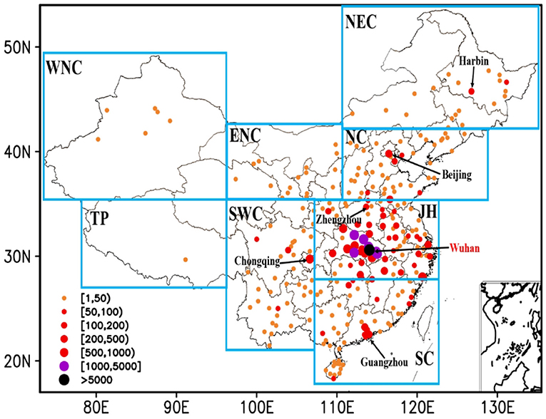
Figure 1. Distribution of confirmed cases in China as of February 25, 2020. The lower right corner is the South China Sea islands. The eight subregions are Northeast China (NEC, 42.25°N−54.75°N, 110.25°E−135.25°E), North China (NC, 35.25°N−42.25°N, 110.25°E−129.75°E), Jianghuai (JH, 27.25°N−35.25°N, 107.25°E−122.75°E), South China (SC, 15.75°N−27.25°N, 107.25°E−122.75°E), Southwest China (SWC, 21.75°N−35.25°N, 97.25°E−107.25°E), Tibetan Plateau (TP, 26.75°N−35.25°N, 97.25°E−107.25°E), West of Northwest China (WNC, 35.25°N−49.75°N, 7.25°E−97.25°E), and East of Northwest China (ENC, 35.25°N−42.75°N, 97.25°E−110.25°E), respectively.

China has a vast territory and can be divided into eight regions based on climate characteristics and geographical location: Northeast China (NEC), North China (NC), the eastern part of Northwest China (ENC), the western part of Northwest China (WNC), the middle and lower reaches of the Yangtze River (JH), South China (SC), Southwest China (SWC), and TP (You et al., 2017). Figure 2 shows the distribution of the daily confirmed cases in the representative provinces and cities of all eight climate regions in China. Similar to Figure 1, there were more confirmed cases in NEC, NC, JH, SC, and SWC and fewer cases in ENC, WNC, and TP. The temporal distributions of the confirmed cases in different provinces and cities were consistent. The confirmed cases began to gradually increase in mid-January, with peaks occurring from the end of January to the beginning of February. Under the strong prevention and control measures taken by governments, the epidemic gradually weakened and basically ended in early March.

FIGURE 2

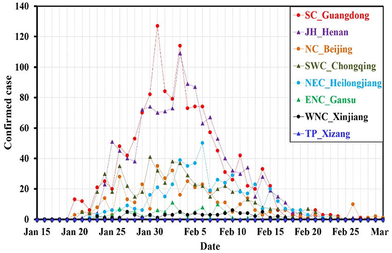
Figure 2. The time series of confirmed cases in typical provinces of different climatic regions in China.

Table 1 lists the linear correlation coefficient (LCC) and Spearman coefficient of rank correlation (SCRC) between the total number of confirmed COVID-19 cases in 30 provincial capitals in China and major meteorological and environmental factors (effective sample size 896). COVID-19 showed linear positive correlations with various air temperature indices and specific humidity and a linear negative correlation with daily average wind speed. Although these correlation coefficients all reached the confidence level of 0.05 or even 0.01, the correlations were not strong (maximum correlation coefficient of 0.164). The linear correlation between COVID-19 and AQI was only 0.051, which was not significant.

TABLE 1

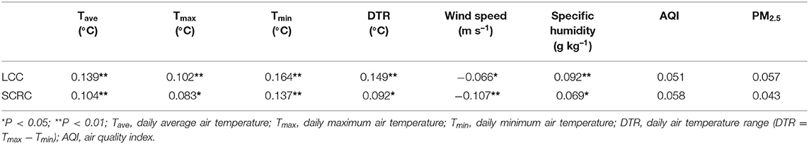
Table 1. The Linear correlations coefficient (LCC) and Spearman coefficient of rank correlation (SCRC) between confirmed cases and meteorological and environmental factors.

Table 1 also provides the Spearman rank correlation coefficients between COVID-19 cases and these factors. According to the test results, Spearman rank correlation coefficient is basically consistent with linear correlation coefficient, which indicates that there are mainly linear correlations between COVID-19 and meteorological factors in China's samples. There were no significant correlations between COVID-19 and AQI and PM_2.5 concentration. For this reason, this paper only discusses linear correlation features in the following analysis. Figure 3A shows the frequency of daily average air temperature and confirmed cases, with a step of 5°C. When the air temperature was lower than 0°C or higher than 15°C, the frequency of an increase in confirmed cases was lower than that of a rise in daily average air temperature; when the air temperature was 0~15°C, the frequency of an increase in confirmed cases was higher than that of a rise in daily average air temperature. This indicates that air temperature of 0~15°C in China favors the spread of COVID-19. In particular, the air temperature data in the range of 5~10°C only accounted for 27.29% of the total air temperature data, but the confirmed cases in this air temperature range accounted for 40.15% of the total COVID-19 cases. Figure 3B shows the scatter plot of the confirmed cases and the daily average air temperature. It can be seen that in different air temperature ranges, the number of confirmed cases had different correlations with air temperature. When the daily average air temperature was lower than −5°C, the number of confirmed cases showed a significant negative correlation with the air temperature, with a correlation coefficient of −0.539. When the daily average air temperature was between −5 and 7°C, the number of confirmed cases was significantly positively correlated with air temperature, with a correlation coefficient of 0.278. When the daily average air temperature was higher than 7°C, the number of confirmed cases was significantly negatively correlated with air temperature, with a correlation coefficient of −0.189. All correlations were higher than the confidence level of 0.01. Therefore, it was not appropriate to use a fixed model to describe the correlations between the number of confirmed cases and air temperature.

FIGURE 3

Figure 3. Frequency distribution (A) and linear correlation (B) between daily average air temperature (T_avg) and confirmed cases in different air temperature ranges.

Similarly, the correlations between the number of confirmed cases and the daily average specific humidity and wind speed in China were statistically analyzed (Figure 4). Under different humidities and wind speeds, the number of confirmed cases was very different. In Figure 4A, when the specific humidity was lower than 3 g kg⁻¹, the frequency of an increase in confirmed cases was lower than that of a rise in specific humidity, so this humidity range was not conducive to the spread of COVID-19. When the specific humidity was >3 g kg⁻¹, the frequency of an increase in confirmed cases was higher than that of a rise in specific humidity. The specific humidity data in the range of 3–5 g kg⁻¹ only accounted for 24.78% of the total data of specific humidity, but the confirmed cases in this range accounted for 40.39% of the total COVID-19 cases, indicating that such humidity conditions are highly favorable for the spread of COVID-19. Data with a specific humidity >11 g kg⁻¹ were mainly collected on the days with precipitation, and these conditions were not conducive to the spread of COVID-19. When the specific humidity was lower than 4 g kg⁻¹, the number of confirmed cases was significantly positively correlated with the atmospheric humidity (r = 0.31). When the specific humidity was >4 g kg⁻¹, there was a significant negative correlation (r = −0.19) between these two.

FIGURE 4

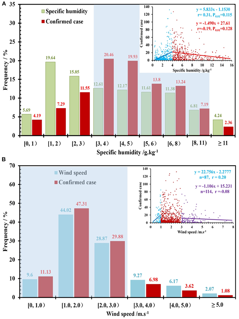
Figure 4. Frequency distribution and linear correlation (inset) between confirmed cases and (A) specific humidity and (B) wind speed.

The distribution of the number of confirmed cases with wind speed is presented in Figure 4B. The data with wind speed <3 m s⁻¹ accounted for 82.49% of the data for daily average wind speed, while the confirmed cases in this wind speed interval accounted for 88.32% of the COVID-19 cases. When the wind speed was > 3 m s⁻¹, the opposite was observed, as the frequency of confirmed cases was lower than that of wind speed data. This means that small wind speed is conducive to the spread of COVID-19. Specifically, when the wind speed was lower than 1 m s⁻¹, the number of confirmed cases was positively correlated with the wind speed (r = 0.20). When the wind speed was >3 m s⁻¹, there was a negative correlation between them (r = −0.08), though it was weak and not significant. When the wind speed was in the range of 1~3 m s⁻¹, there was no definite relationship between the number of confirmed cases and wind speed.

There are great geographical and climatic differences across China (You et al., 2017). Figure 2 shows that the COVID-19 outbreak process in each region has a similar pattern, but it is not clear whether it also has a similar response pattern with meteorological and environmental factors. In this study, a representative city in each climate region (NEC: Harbin; NC: Beijing; JH: Zhengzhou; SC: Guangzhou; SWC: Chongqing; Figure 1) with good data was selected for analysis. Table 2 shows that air temperature was the most significant factor affecting COVID-19. Whether in the cold and dry northern cities of Beijing and Harbin, or the relatively warm southern cities of Guangzhou and Chongqing, or the central city of Zhengzhou, where the climate conditions are somewhere in between, the number of confirmed cases was stably correlated with daily average air temperature and daily minimum air temperature (P < 0.05). Among them, the correlation between the number of confirmed cases and daily maximum air temperature in Beijing and Harbin, the northern cities, was relatively high (P < 0.05). This may be because air temperature was a relatively stable variable. During the relatively short period of the epidemic, the air temperature variations in these cities rarely exceeded the threshold (Figure 3). However, the number of confirmed cases was not well-correlated with changes in air temperature and daily air temperature range, which means that a long period with appropriate air temperature could have a greater impact on COVID-19 than a period with sudden temperature changes. The number of confirmed cases was weakly and non-significantly correlated with wind speed and specific humidity, which might be related to the relatively large variations in these meteorological factors during this period. The statistical results showed that the correlations between the number of confirmed cases and wind speed and specific humidity were not consistent across different ranges (Figure 4). In addition, the correlation between the AQI and COVID-19 remained weak.

TABLE 2

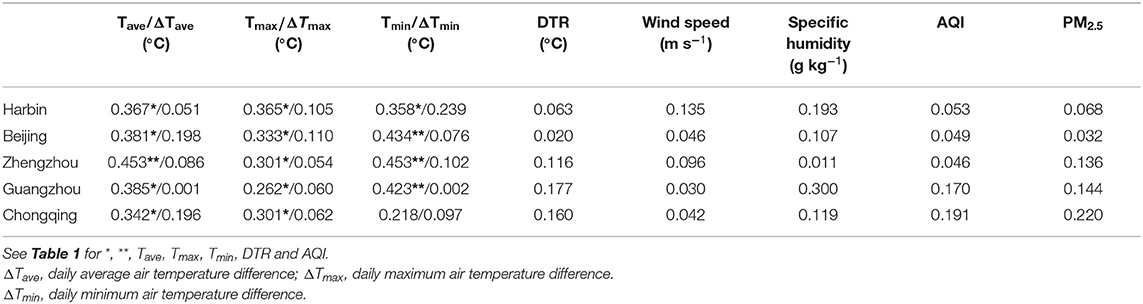
Table 2. The Linear correlations between confirmed cases and meteorological and environmental factors.

Causality Test

As a hypothesis testing scheme, the Granger causality test is generally used to test two groups of variables with good correlation, so as to further judge whether there is causal correlation between them. Given that only the correlation between the number of confirmed cases and the air temperature in the representative cities reached significance standard, the Granger causality test was used to determine whether there was a causal relationship between them. The Granger causality test was performed by EViews 6.0.

The ADF test (Table 3) showed that both daily average air temperature and confirmed cases were all stationary series in these cities (P < 0.01), so the Granger causality test could be directly performed. Table 4 shows that when Lag took k = 1, for the northern cities of Harbin and Beijing and the southern city of Guangzhou, the F statistics were 1.290, 1.647, and 1.098, and P-values were 0.026, 0.020, and 0.030, respectively. That is, the null hypothesis was rejected with the probability of P < 0.05, and the test conclusion was that daily average air temperature was the Granger cause of the number of confirmed cases; moreover, it shows that the air temperature in these cities not only highly correlated with the number of confirmed cases that day but also has a strong indication of the number of confirmed cases the next day. For the central city of Zhengzhou and southwestern city of Chongqing, when the probability of P < 0.05 or P < 0.1, the test results showed that daily average air temperature was not the Granger cause of the number of confirmed cases. It indicated that although the air temperature in these cities had a high correlation with the number of confirmed cases on the same day, it was not indicative of the number of confirmed cases the next day.

TABLE 3

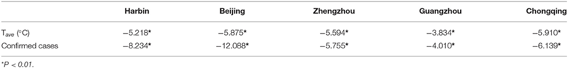
Table 3. Augmented Dickey-Fuller test results for daily average air temperature (T_ave) and confirmed cases in 5 cities.

TABLE 4

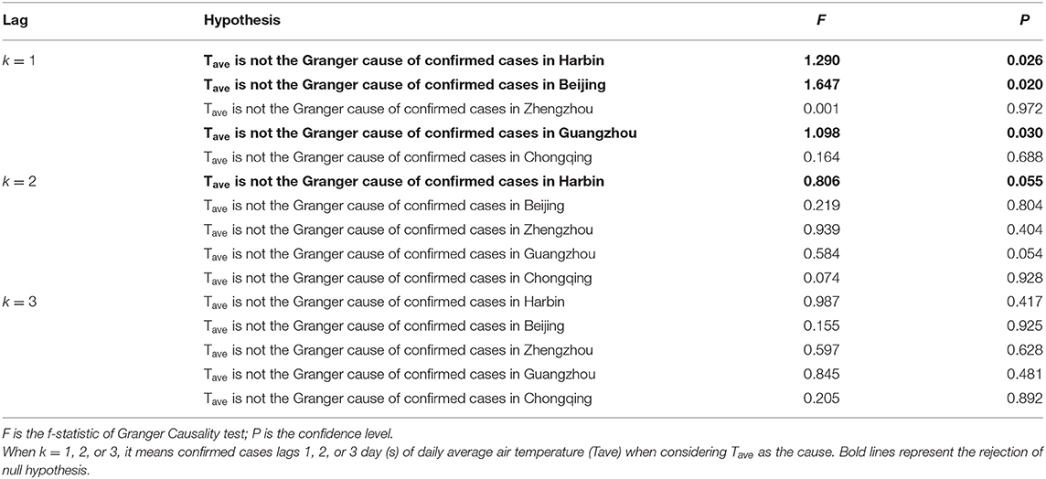
Table 4. Granger causality test results.

When Lag took k = 2, only the test for Harbin could reject the null hypothesis with a probability of P < 0.1, which suggested that air temperature still affected the number of confirmed cases every other day, but the indication significance became weaker. On the other hand, tests for other cities could not reject the null hypothesis. When Lag took k = 3, no causality can be tested in all cities.

Conclusion and Discussion

The impact of meteorological conditions on COVID-19 is a controversial issue. The analysis of this paper found that the correlations between COVID-19 and air temperature, humidity, and wind speed in major cities in China were significantly different in different climate backgrounds. Therefore, it is inappropriate to use a fixed model to describe the relationships between COVID-19 and meteorological factors. Generally, high humidity, low wind speed, and relatively low air temperature were conducive to the spread of COVID-19.

Affected by sample size and geographical location, some research results seem inconsistent. For example, Xie and Zhu (2020) based on data from 122 cities in China found that COVID-19 confirmed cases increased approximately linearly when the daily average air temperature <3°C, and it tended to be flat when daily average air temperature was above 3°C. Luo et al. (2020) reported that COVID-19 can still spread under warm and humid conditions. All this information can be considered as a subset of Figure 3B in this paper, indicating that more samples are needed to obtain a more comprehensive understanding. Recently, Huang et al. (2020) pointed out that the optimal temperature for COVID-19 spread was 5~15°C, and 70% of confirmed cases worldwide occurred between 5 and ~15°C, which is similar to this paper. In addition to Hubei Province, China still has 58.2% of cases in this temperature range, but only 43.2% of the temperature data (Figure 3A). This indicates that although human prevention and control measures play an important role in the spread of the virus, signals of climate impact can still be detected on a global scale, and capturing these signals will help us better respond to the COVID-19 epidemic.

This paper also applied the Granger causality test to detect any causal connection between COVID-19 and air temperature in five representative cities. The results show that with a confidence level of 0.05, there is a causal relationship between the daily average air temperature and the number of confirmed cases on the next day in some cities, such as Harbin, Beijing, and Guangzhou. With a confidence of 0.1, the air temperature in Harbin was still indicative of the number of confirmed cases on every other day. However, this phenomenon was not universal due to geographical differences. During the epidemic period, the air temperatures in Harbin, Beijing, and Guangzhou were −25~10, −6~6, and 8~20°C, respectively, and the number of COVID-19 confirmed cases increased or decreased monotonically with temperature in these temperature ranges (Figure 3B). In Zhengzhou and Chongqing, there was no similar correspondence, which suggested that only relying on the correlation coefficient may mislead some incorrect conclusions.

Due to the active and effective prevention and control measures taken by the Chinese government, the epidemic period of COVID-19 in China is relatively short (Figure 2). In order to ensure there were sufficient statistical samples in cities of different geographical climate regions, this study analyzes the correlations between COVID-19 and meteorological and environmental factors during the entire epidemic period in China. Are these correlations consistent at different stages of an epidemic? Further research is required. Although a previous study has reported that ambient air pollution has a significant impact on respiratory diseases (Ma et al., 2018), statistics in this study show that the linear correlation coefficient and Spearman rank correlation coefficient between the AQI (PM_2.5) and COVID-19 are weak on both national and regional scales. Perhaps, there is some unknown and complex connection between COVID-19 and aerosols, and its mechanism still needs further study.

Data Availability Statement

The original contributions presented in the study are included in the article/supplementary materials, further inquiries can be directed to the corresponding author/s.

Author Contributions

ZZ performed the data analysis, data interpretation, and wrote the paper. JD contributed to data analysis, interpretation, and paper writing. CC and HG contributed to the collection and quality control of the data. All authors contributed to improving the paper.

Funding

This study was supported by Beijing Natural Science Foundation (8202022) and the National Natural Science Foundation of China (41575010).

Conflict of Interest

The authors declare that the research was conducted in the absence of any commercial or financial relationships that could be construed as a potential conflict of interest.

References

Barnett, T. P., Hegerl, G. C., Knutson, T., and Tett, S. (2000). Uncertainty levels in predicted patterns of anthropogenic climate change. J. Geophys. Res. Atmos. 105, 15525–15542. doi: 10.1029/2000JD900162

CrossRef Full Text | Google Scholar

Carlson, C. S., Eberle, M. A., Kruglyak, L., and Nickerson, D. A. (2004). Mapping complex disease loci in whole-genome association studies. Nature 429, 446–452. doi: 10.1038/nature02623

PubMed Abstract | CrossRef Full Text | Google Scholar

Dalziel, B. D., Kissler, S., Gog, J. R., Viboud, C., Bjørnstad, O. N., Metcalf, C. J., et al. (2018). Urbanization and humidity shape the intensity of influenza epidemics in US cities. Science 362, 75–79. doi: 10.1126/science.aat6030

CrossRef Full Text | Google Scholar

Drosten, C., Günther, S., Preiser, W., Werf, S., Brodt, H. R., Becker, S., et al. (2003). Identification of a novel coronavirus in patients with severe acute respiratory syndrome. N. Engl. J. Med, 348, 1967–1976. doi: 10.1056/NEJMoa030747

PubMed Abstract | CrossRef Full Text | Google Scholar

Granger, C. W. J. (1980). Testing for causality: a personal view point. J. Econ. Dyn. Control 2, 329–352. doi: 10.1016/0165-1889(80)90069-X

CrossRef Full Text | Google Scholar

He, Z. C., Xiao, L. S., Guo, Q. H., Liu, Y., Mao, Q. Z., and Kareiva, P. (2020). Evidence of causality between economic growth and vegetation dynamics and implications for sustainability policy in Chinese cities. J. Clean. Prod. 251:119550. doi: 10.1016/j.jclepro.2019.119550

CrossRef Full Text | Google Scholar

Houghton, J. T., Ding, Y., and Griggs, D. G. (2001). Climate Change 2001: The Scientific Basis. Contribution of Working Group I to the Third Assessment Report of the IPCC. Cambridge: Cambridge University Press.

Google Scholar

Huang, Z. W., Huang, J. P., Gu, Q. Q., Du, P. G., Liang, H. B., and Dong, Q. (2020). Optimal Temperature Zone for the Dispersal of COVID-19. Science of the Total Environment. doi: 10.1016/j.scitotenv.2020.139487

PubMed Abstract | CrossRef Full Text | Google Scholar

Joliffe, I. T. (1983). Why do we get spurious correlation in climatology: some explanations. Int. Meet. Stat. Climatol. 16, 1–6.

Kissler, S. M., Tedijanto, C., Goldstein, E., Grad, Y. H., and Lipsitch, M. (2020). Projecting the transmission dynamics of SARS-CoV-2 through the post pandemic period. Science 368, 860–868. doi: 10.1126/science.abb5793

CrossRef Full Text | Google Scholar

Li, S. P., Wang, H. L., and Feng, J. F. (2004). Analysis of Non-linear correlation of the concentration of harmful algal with environmental factor in Bohai Bay. Ocean Technol. 23, 82–84.

Liu, Q., Tan, Z. M., Sun, J., Hou, Y. Y., Fu, C. B., and Wu, Z. H. (2020). Changing rapid weather variability increases influenza epidemic risk in a warming climate. Environ. Res. Lett. 15:044004. doi: 10.1088/1748-9326/ab70bc

CrossRef Full Text | Google Scholar

Liu, Y., Ning, Z., Chen, Y., Guo, M., Liu, Y. L., Gali, N. K., et al. (2020). Aerodynamic Analysis of SARS-CoV-2 in two Wuhan Hospitals. Nature 582, 557–560. doi: 10.1038/s41586-020-2271-3

PubMed Abstract | CrossRef Full Text | Google Scholar

Luo, C., Yao, L., Zhang, L., Yao, M. C., Chen, X. F., Wang, Q. L., et al. (2020). Possible Transmission of Severe Acute Respiratory Syndrome Coronavirus 2. (SARS-CoV-2) in a Public Bath Center in Huai'an, Jiangsu Province, China. JAMA Netw. Open 3:e204583. doi: 10.1001/jamanetworkopen.2020.4583

PubMed Abstract | CrossRef Full Text | Google Scholar

Ma, Y. L., Zhao, Y. D., Liu, J. T., He, X. T., Wang, B., Fu, S. H., et al. (2020). Effects of Temperature Variation and Humidity on the Mortality of COVID-19 in Wuhan. MedRxiv [Preprint]. doi: 10.1101/2020.03.15.20036426

CrossRef Full Text | Google Scholar

Ma, Y. X., Yang, S. X., Zhou, J. D., Yu, Z. A., and Zhou, J. (2018). Effect of ambient air pollution on emergency room admissions for respiratory diseases in Beijing, China. Atmos. Environ. 191, 320–327. doi: 10.1016/j.atmosenv.2018.08.027

CrossRef Full Text | Google Scholar

Mosedale, T. J., Stephenson, D. B., and Collins, M. (2006). Granger causality of coupled climate processes: Ocean feedback on the North Atlantic oscillation. J. Clim. 19, 1182–1194. doi: 10.1175/JCLI3653.1

CrossRef Full Text | Google Scholar

Tellier, J. R. (2009). Aerosol transmission of influenza a virus: a review of new studies. J. R. Soc. Interf. 6, S783–S790. doi: 10.1098/rsif.2009.0302.focus

PubMed Abstract | CrossRef Full Text | Google Scholar

Triacca, U. (2001). On the use of Granger causality to investigate the human influence on climate. Theor. Appl. Climatol. 69, 137–138. doi: 10.1007/s007040170019

CrossRef Full Text | Google Scholar

Wang, J. Y., Tang, K., Feng, K., and Lv, W. F. (2020). High temperature and high humidity reduce the transmission of COVID-19. SSRN [Preprint]. doi: 10.2139/ssrn.3551767

PubMed Abstract | CrossRef Full Text | Google Scholar

Wang, W., Anderson, B. T., Kaufmann, R. K., and Myneni, R. B. (2004). The relation between the North Atlantic Oscillation and SSTs in the North Atlantic Basin. J. Clim. 17, 4752–4759. doi: 10.1175/JCLI-3186.1

CrossRef Full Text | Google Scholar

Wu, G. P., and Zhang, D. Y. (2012). Nonlinear dependence of anomalous resistivity on the reconnecting electric field in the Earth's magnetotail. Chin. Sci. Bull. 57, 1449–1454. doi: 10.1007/s11434-011-4902-4

CrossRef Full Text | Google Scholar

Xie, J. G., and Zhu, Y. J. (2020). Association between ambient temperature and COVID-19 infection in 122 cities from China. Sci. Total Environ. 724:138201. doi: 10.1016/j.scitotenv.2020.138201

PubMed Abstract | CrossRef Full Text | Google Scholar

You, Q. L., Jiang, Z. H., Kong, L., Wu, Z. W., Bao, Y. T., Kang, S. C., et al. (2017). A comparison of heat wave climatologies and trends in China based on multiple definitions. Clim. Dyn. 48, 3975–3989. doi: 10.1007/s00382-016-3315-0

CrossRef Full Text | Google Scholar

Yu, Q. W., Liu, Q. H., Feng, Z. X., Deng, X. J., Mai, B. R., Li, F., et al. (2016). Exploring granger causality of global carbon dioxide concentration and the urbanization effect for temperature trends in Hong Kong over the period 1886-2012. J. Trop. Meteorol. 32, 855–863. doi: 10.16032/j.issn.1004-4965.2016.06.007

CrossRef Full Text | Google Scholar

Zheng, Z. F., Xu, G. R., Yang, Y. J., Wang, Y. T., and Li, Q. C. (2018). Statistical characteristics and the urban Spillover effect of haze pollution in the circum-Beijing region. Atmos. Pollut. Res. 9, 1062–1071. doi: 10.1016/j.apr.2018.04.004

CrossRef Full Text | Google Scholar