A Physics-Aware Neural Network Approach for Flow Data Reconstruction From Satellite Observations

1. Introduction

The formation of observable mesoscale vortex patterns on satellite imagery is driven by atmospheric processes. Certain structures, such as Karman vortex streets forming in the stratocumulus-topped wake of a mountainous islands, bear resemblance to patterns observable in laboratory flows. Such flow structures have been studied based on satellite measurements since the 1960s (Hubert and Krueger, 1962; Chopra and Hubert, 1965; Young and Zawislak, 2006). Recent advances in remote sensing (Geerts et al., 2018) enabled the retrieval of high-resolution wind fields at kilometer-scale (Horváth et al., 2017, 2020), which is a necessary requirement for the analysis of atmospheric processes in turbulent environments. While operational wind products based on the Advanced Baseline Imager (ABI) onboard the Geostationary Operational Enrivonmental Satellite-R (GEOS-R) (Schmit et al., 2017) provide a 7.5 km resolution, Horváth et al. (2020) utilized the internal wind vectors at 2.5 km resolution in their study of vortex patterns in the wake of Guadalupe Island off Baja California on 9 May 2018, which were combined with MODIS-GEOS wind products offering stereo cloud-top heights and semi-independent wind validation data (Carr et al., 2019). Utilizing such high resolutions is necessary for the analysis of small-scale structures, but comes at the price of an increased level of measurement noise, which is accompanied by general uncertainty in regions without or with only few clouds. Disambiguation of possible flow configurations based on imperfect measurement data is thereby challenging. At present, such spaceborne measurements have been cleaned with median filters, smoothing, and thresholding of unreasonably large velocity components (Horváth et al., 2020). Thus, current approaches to reconstruct missing or uncertain information are based on assumptions about the signal smoothness, and do not yet incorporate that the wind fields are the result of fluid dynamical processes. Such physical regularizations, however, are more difficult to model.

Data-driven regularization and data recovery with neural networks offer great potential for data completion tasks. A main challenge is to include physics knowledge in the network design, such that the reconstruction follows the solution of the fluid dynamic equations. Cloud satellite imagery may contain large areas of missing or uncertain data, and high noise levels. Further, the fluid dynamics are affected by the topography. Therefore, the data inference must be powerful enough to generate accurate results even in such challenging settings. Neural networks have excellent properties for data completion: they are universal approximators, and are able to efficiently combine data-driven and physics-based regularizations. Data reconstructed with neural networks, however, typically lack details due to the convolution operations, which manifests as degraded and smoothed flow details. In this paper, we present a novel neural network architecture for 2-D velocity fields extracted from satellite imagery. Our method uses physically-inspired regularization, leveraging surrogate simulations that are generated in the full three dimensional space, which enables a more precise approximation of the transport phenomena. The inference time of our approach is fast, offering new applications for predicting large scale flows in meteorological settings.

Deep learning approaches are currently studied with great interest in climate science in a number of different topics, including convection (O'Gorman and Dwyer, 2018), forecasting (Weyn et al., 2019), microphysics (Seifert and Rasp, 2020), empirical-statistical downscaling (Baño-Medina et al., 2020), and radiative transfer (Min et al., 2020). Estimating missing flow field data has many similarities with the image inpainting task commonly studied in computer vision, as it is essentially a scene completion process using partial observations. The recent success of learning-based image inpainting algorithms demonstrates the capability of deep neural networks to complete large missing regions in natural images in a plausible fashion. Pathak et al. (2016) used Context Encoders as one of the first attempts for filling missing image data with a deep convolutional neural network (CNN). CNN-based methods are attractive due to their ability to reconstruct complex functions with only few sparse samples while being highly efficient. The follow-up work by Iizuka et al. (2017) proposed a fully convolutional network to complete rectangular missing data regions. The approach, however, still relied on Poisson image blending as a post-processing step. Yu et al. (2018) introduced contextual attention layers to model long-range dependencies in images and a refinement network for post-processing, enabling end-to-end training. Zeng et al. (2019) extended previous work by extracting context attention maps in different layers of the encoder and skip connect attention maps to the decoder. These approaches all include adversarial losses computed from a discriminator (Goodfellow et al., 2014) in order to better reconstruct visually appealing high frequency details. However, high frequency details from adversarial losses can result in mismatches from ground truth data (Huang et al., 2017), which can potentially predict missing data that diverge from physical laws. Liu et al. (2018) designed partial convolution operations for image inpainting, so that the prediction of the missing pixels is only conditioned on the valid pixels in the original image. The operation enables high quality inpainting results without adversarial loss. Inpainting approaches have also been successfully used for scene completion and view path planning using data from sparse input views. Song et al. (2017) used an end-to-end network SSCNet for scene completion and Guo and Tong (2018) a view-volume CNN that extracts geometric features from 2D depth images. Zhang and Funkhouser (2018) presented an end-to-end architecture for depth inpainting, and Han et al. (2019) used multi-view depth completion to predict point cloud representations. A 3D recurrent network has been used to integrate information from only a few input views (Choy et al., 2016), and Xu et al. (2016) used spatial and temporal structure of sequential observations to predict a view sequence. We base our method on previous deep learning architectures for image inpainting, namely a U-Net (Ronneberger et al., 2015) with partial convolutions (Liu et al., 2018). Utilizing that we are dealing with velocity fields instead of images, we further include a physically-inspired loss function to better regularize the predicted flow data. Neural networks have also recently been applied to fluid simulations. Applications include prediction of the entire dynamics (Wiewel et al., 2019), reconstruction of simulations from a set of input parameters (Kim et al., 2019b), interactive shape design (Umetani and Bickel, 2018), inferring hidden physics quantities (Raissi et al., 2018), and artistic control for visual effects (Kim et al., 2019a). A comprehensive overview of machine learning for fluid dynamics can be found in Brunton et al. (2020).

2. Method

In this paper, we demonstrate that the reconstruction of high-quality wind fields from noisy, uncertain and incomplete satellite-based wind retrievals based on GEOS-R measurements (Schmit et al., 2017) can be learned by a neural network from numerical simulations of realizable fluid flows. The training and evaluation of such a supervised approach is, however, challenging due to the lack of ground truth data. Thus, in a first step we numerically simulate fluid flows, which we synthetically modify to account for uncertainty and lack of measurements. The flow configurations must thereby be chosen carefully to sample the space of possible fluid configurations uniformly. Simply using off-the-shelf reanalysis simulations (Hersbach et al., 2020) would bias the network to perform best on very common fluid flow configurations, leading to poor results in the exceptional situations that are most interesting to study. For this reason, we generate fluid flow configurations in a controlled manner suitable for supervised machine learning. Afterwards, we analyze the performance of our model on satellite wind retrievals in the wake of Guadalupe island by Horváth et al. (2020) and compare those with linear reconstructions obtained via least-squares minimization. Our neural network has similarities with image inpainting approaches, mainly stemming from both sharing a scene completion process using partial observations. The major difference between flow field and image inpainting is that flow field data inherently follows the solution of the fluid dynamic equations. Hence, existing image inpainting algorithms can easily fail in physics-aware completion tasks as they never aim to capture the underlying physical laws. The presented flow inpainting method therefore considers the mathematical equations that model the fluid phenomena in the design of the network architecture and loss functions. The network is designed such that large areas of missing data with and without obstacles can be inferred. In the next sections, we are going to detail how we designed our network architecture, along with challenges and necessary modifications that were made to support fluid flow data.

2.1. Network Architecture

Our goal is to train a network that can fill empty regions of velocity fields. The input scheme is similar to standard image inpainting tasks. For a given 2D velocity field ${\overrightarrow{u}}_{in}$ with missing fluid regions represented by a binary mask M (0 for empty and 1 for known regions), the network predicts the inpainted velocity field $\widehat{\overrightarrow{u}}$. Existing consistency checks, such as wind speeds not exceeding 8 m/s can be incorporated directly by the mask. The network for fluid data completion consists of three main parts: an encoder, dense blocks, and a decoder. The encoder-decoder pair follows a U-Net structure (Ronneberger et al., 2015) shown in Figure 1. It first encodes the original velocity field by reducing the spatial resolution progressively, later decoding it by increasing the resolution until it matches the original size. This way, features are extracted on all scales. The U-Net includes skip connections that forward these scale-dependent features from the encoding phase to the decoding phase in order retain the locality of high-frequent information. To improve the quality of the results obtained by the U-Net further, we add Dense Blocks (Huang et al., 2017) at the bottleneck to enrich the feature representation.

FIGURE 1

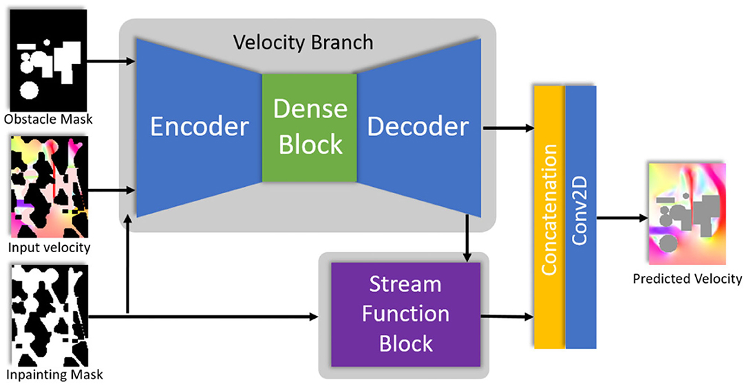
Figure 1. Our network architecture uses a U-Net with Dense Blocks to predict velocity fields. A stream function block implemented through another Dense Block can be added for incompressible flow data. Our synthetic data experiments use the stream function block, while the results of the Guadalupe island do not, since they are slices of 3-D incompressible flows, and thus, not divergent free.

Each layer of the network is implemented by replacing the standard convolution operations with modified partial convolutions (Liu et al., 2018). The modified partial convolution at every location is defined as

$\begin{array}{l}{x}^{\prime }=\{\begin{array}{ll}{\text{C}}^T(\text{X }·\text{ M})\frac{sum(1)}{sum(\text{M})}+b,& \text{if }sum(\text{M})>1\\ 0,& \text{otherwise}\end{array}\\ m^{\prime }=\{\begin{array}{cc}1,& \text{if }sum(\text{M})>1\\ 0,& \text{otherwise}\end{array}& (1)\end{array}$

where x′ and m′ are the layer output and updated mask, respectively. C represents the convolution filter weights and b refers to its corresponding bias. X are the feature values for the current input window. M is the corresponding binary mask. X·M is an element-wise multiplication, and 1 has the same shape as M with all the elements equal to 1. The key difference between partial convolution and normal convolution is to multiply X and M element-wisely. In this way, the output only depends on the unmasked input values. A scaling factor $\frac{sum(1)}{sum(\text{M})}$ adjusts for varying amount of unmasked input values, leading to sharper velocity profiles in the reconstructed field. For incompressible flow fields we can add a stream function block as shown in Figure 1. The resulting velocity field can then be reconstructed from the predicted stream function field Ψ(x, y) by u = ∇ × Ψ. We refer to the Appendix for more detailed information about the network architecture and the training setup.

2.2. Loss Functions

It is important to define a new set of supervised loss functions to model physical properties and constraints for fluid flow data. Let $\widehat{\text{u}}$ be the predicted velocities and u be the ground truth velocities. We keep the L¹ reconstruction loss as it can efficiently reconstruct low-frequency information:

$\begin{array}{ll}{L}_{vel}=\left|\right|(\widehat{\text{u}}-\text{u})·\text{M}|{|}_1+{\alpha }_{vel}||(\widehat{\text{u}}-\text{u})·(1-\text{M})|{|}_1,& (2)\end{array}$

where α_vel is a scale factor that weights between empty and known regions. We use α_vel > 1 to emphasize better reconstructions on regions where the flow information is missing. Inspired by Kim et al. (2019b), we additionally minimize the difference of the velocity field Jacobian between ground truth and predicted velocity fields. With a sufficiently smooth flow field data set, high-frequency features of the CNN are potentially on the null space of the L¹ distance minimization (Kim et al., 2019b). Thus, matching the Jacobians helps the network to recover high-frequency spectral information, while it also regularizes the reconstructed velocity to match ground truth derivatives. The velocity Jacobian J(u) is defined in 2D as

$\begin{array}{ll}J(\text{u})=\left(\begin{array}{cc}\frac{\partial {\text{u}}_x}{\partial x}& \frac{\partial {\text{u}}_x}{\partial y}\\ \frac{\partial {\text{u}}_y}{\partial x}& \frac{\partial {\text{u}}_y}{\partial y}\end{array}\right),& (3)\end{array}$

and the corresponding loss function is simply given as the L¹ of vectorized Jacobian between predicted and ground truth velocities:

$\begin{array}{ll}{L}_{jac}=\left|\right|(J(\widehat{\text{u}})-J(\text{u}))·\text{M}|{|}_1+{\alpha }_{jac}||(J(\widehat{\text{u}})-J(\text{u}))·(1-\text{M})|{|}_1.& (4)\end{array}$

Additionally, we compute a loss function that matches the vorticity of predicted and ground truth velocities. The vorticity field describes the local spinning motion of the velocity field. Similarly to the Jacobian loss, our vorticity loss acts as a directional high-frequency filter that helps to match shearing derivatives of the original data, enhancing the capability of the model to properly match the underlying fluid dynamics. The vorticity loss is defined as:

$\begin{array}{ll}{L}_{vort}=\left|\right|(\nabla \times \widehat{\text{u}}-\nabla \times \text{u})·\text{M}|{|}_1+{\alpha }_{vort}||(\nabla \times \widehat{\text{u}}-\nabla \times \text{u})·(1-\text{M})|{|}_1.& (5)\end{array}$

Incompressible flows should have zero divergence, but numerical simulations often produce results that are not strictly divergence-free due to discretization errors. As we inpaint missing fluid regions, we aim to minimize the divergence on the predicted fields by

$\begin{array}{ll}\begin{array}{c}{L}_{div}=\left|\right|\nabla ·\widehat{\text{u}}|{|}_1.\end{array}& (6)\end{array}$

Lastly, all losses modeled by the network are based on the L₁ distance function. Distance-based loss functions are known for undershooting magnitude values, creating results that are visibly smoother. This is especially visible for the inpainting task when we substitute original measured values back into the velocity field $\widehat{\overrightarrow{u}}$ reconstructed by the network. Therefore, we employed a magnitude of the gradient as our last loss function to produce inpainted results that have less discrepancies when using original measured values for known regions:

$\begin{array}{ll}{L}_{mag}=\left|\right|(\nabla \left|\right|\widehat{\text{u}}·(1-M)+\text{u}·M|{|}_2)·{\text{W}}_{mag}|{|}_1.& (7)\end{array}$

The magnitude of the gradient loss needs a special weighting function W_mag that depends on the mask interface, since if used indistinguishably it can also quickly degenerate the convergence of the network. This weighting function is computed based on the morphological gradient of the mask, which is the difference between the mask dilation and its erosion, which yields a 1-ring mask boundary. We expand the mask boundary continuously by dilation, in order to fill the regions of missing information. As the mask is expanded internal weights are assigned based on the iteration of the dilation–initial iterations have higher values that decay as iterations progress. This is similar to compute a level-set distance function from a missing region to the mask boundary, however our implementation is computationally more effective. The mask is bounded from [1, 3], with higher values closer to the mask boundary.

Notice that all our loss functions, excluding the divergence-free one, employ weights to known and unknown regions. This is a common strategy in inpainting works, and we empirically found that for our data sets α_vel = α_jac = α_vort = 6 to yield the best results. Other loss functions, such as perceptual loss and style loss (Liu et al., 2018) are not suited for completing flow field data, since they match pre-learned filters from image classification architectures.

2.3. Encoding Obstacles

The interaction between fluid and solid obstacles is crucial for fluid dynamics applications, as the interaction creates shear layers that drive the formation of vortices. To incorporate solid obstacle information as prior knowledge to the network, we concatenate a binary mask O indicating whether a solid obstacle occupies a cell (1) or not (0) as an extra input channel. In order to properly propagate the obstacle information to all network layers, O is concatenated to previous layers' output as input to the current layer. To account for resolution change between network layers, we downsample and upsample the obstacle map O using average pooling.

3. Results

We show that the learning-based reconstruction is especially powerful in handling large areas of missing or occluded data, outperforming traditional models for data recovery. We evaluate our method on numerically-simulated flows, and additionally apply it to the Guadalupe Island case study.

3.1. Inpainting of Synthetic Data

Due to the lack of publicly available flow data sets captured from real-world experiments, we trained our model on synthetic data. We generated fluid velocity fields with a numerical incompressible flow solver [Mantaflow (Thuerey and Pfaff, 2018)] and used the stream function block in the training. Each data sample consists of a 2-dimensional ground truth vector field $\overrightarrow{u}$, as well as the empty regions and obstacles masks M and O. To use the data sample in both training and testing, we apply empty regions mask M on both velocity component through element-wise multiplication to obtain the input velocity to the model ${\overrightarrow{u}}_{in}=\overrightarrow{u}·\text{M}$. The model concatenates the input velocity ${\overrightarrow{u}}_{in}$, empty regions mask M and obstacle mask O as input, and outputs the predicted velocity field $\widehat{\overrightarrow{u}}$. Our synthetic flow data set for this task completion is computed on a grid resolution of 128 × 96. The wind tunnel data set implements a scene with transient turbulent flow around obstacles. We define inflow velocities at bottom and top regions of the domain, while the remaining two sides (left and right) are set as free flow (open) boundary conditions. The inflow speed is set to random values, and 12 obstacles varying between spheres, rectangles and ellipses are randomly positioned, yielding a total of 25,500 unique simulation frames. Examples of velocity fields generated by this simulation setup can be seen in Figure 2. We split the whole data set into training (78%), validation (10%), and test (12%) data sets. Each split of the data set comes from a different set of simulation runs. Models are trained on the training set and are compared on the validation set. Later, we report visual results on the test set.

FIGURE 2

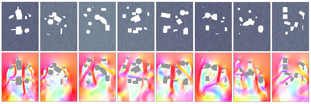
Figure 2. Several simulation examples for generating the wind tunnel data set. The images above show the line integral convolution (LIC) plots, while images below show HSV color coded velocity fields.

During training, different types of empty region masks are generated on the fly with empty to filled area region ratios that vary randomly between 10 and 99%. The gradient magnitude mask W_mag is also automatically generated for all masks used in the training phase. We model three different types of masks for this task: uniform random noise masks mimic possible sampling noise from real-world velocity measurements; scan path masks simulate paths of a velocity probing; and large region masks model large occluded areas that are not reachable by probes or measurement devices. Illustrations of these types of masks can be seen in Figures 3, 4.

FIGURE 3

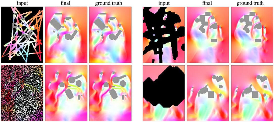
Figure 3. Examples of predictions using the wind tunnel data set. From left to right of each example: masked velocity input, output of our network, ground truth velocity.

FIGURE 4

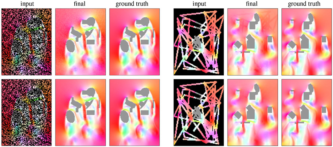
Figure 4. Results without (top) and with (bottom) the magnitude of the gradient loss (Equation 7). The latter removes visible artifacts at mask boundaries.

Results of our approach can be seen in Figures 3, 4 bottom. The results are generated by taking simulations from the test data set, applying an input mask and feeding as the input of the network, along with the obstacle boundary mask. Our results demonstrate that our deep learning approach is able to plausibly reconstruct flows even in regions with large occlusions. In our evaluations we found that the use of the Dense Block and the combination of the proposed losses yield best results in terms of Mean Absolute Error. The effect of the magnitude of the gradient loss (Equation 7) is particularly interesting as it enforces smooth magnitude transitions in the output and hence reduces artifacts. This is demonstrated visually in Figure 4, where the top and bottom rows were computed without and with magnitude of the gradient loss, respectively. Without using this loss, there are noticeable differences in the magnitude of the recovered values, and the masks can be seen in the final reconstruction.

3.2. Inpainting of Velocity Measurements Obtained by Optical Flow

We further evaluate the model on a real-world data set consisting of reconstructed velocity fields from satellite imagery of the atmospheric vortex street behind Guadalupe Island (Horváth et al., 2020). Figure 5 shows the satellite imagery on 9 May 2018 with the vortex generating structure behind the island. Based on 2.5 km GEOS-R observations, patches of 5 × 5 were tracked over time to reconstruct temporal correspondences, resulting in a sequence of 96 time steps with spatial resolution of 6.3 km and 5 min. The reconstructed velocity fields are noisy and lack information outside of the satellite's field of view as well as in areas where the cloud tracking algorithm fails to produce valid results. We show that our model is capable of reconstructing and preserving the vortex generating structure behind Guadalupe Island, whereas conventional methods fail to reconstruct these structures at such detail. The noise of the real-world data set is successfully removed by the network, generating smooth flow predictions. We demonstrate that physical quantities, such as the vorticity is more accurately captured by our model, especially directly in the wake of the island.

FIGURE 5

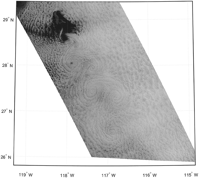
Figure 5. Radiance map of Guadalupe island on 9 May 2018 at 14:37 UTC.

For this task, we generated a three dimensional flow with a voxelized representation of the Guadalupe island geometry immersed in the domain. This setup allows a more realistic flow over the Guadalupe island boundaries, in which the flow can go above and around the island. Since the velocity fields reconstructed from satellite observations are 2-D, we only use the velocity components u and v from the simulated data set at about 800 m above sea level. We also omitted the stream function block of the network and the divergence loss term, since we are evaluating 2-D slices of a 3-D velocity field, which are not guaranteed to be incompressible on the sliced plane. For the scene boundaries, we set the left and bottom with inflow velocities, right and top with outflow conditions. The other two boundaries (above and below) are modeled with free-slip boundary conditions.

The masks used for completing this data set are obtained from evaluating noise patterns that emerge in cloud remote sensing. In Figure 6, left, we show how those patterns appear due to errors in the cloud tracking algorithm. We extract many of these samples to generate masks that are similar to the ones that are going to be used to complete the velocity field. This is done by two filtering steps for removing velocities exceeding 8 m/s and noise (Figure 6, center and right).

FIGURE 6

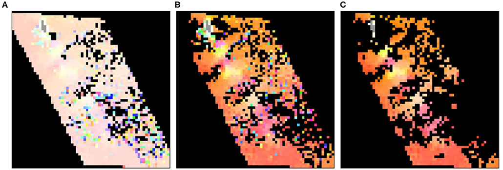
Figure 6. A real-world data sample: Original data (A), filtered data to remove velocities exceeding 8 m/s (B), and removal of local noise (C).

A real-world sample reconstructed with our method is shown in Figure 7. The reconstructed vector field is smooth and completes the real-world sample plausibly. We compare our model with a least-squares approximation, minimizing:

$\begin{array}{ll}\begin{array}{c}E={\displaystyle {\int }_{{M}}}\left|\right|\widehat{\text{u}}-\text{u}|{|}^2\text{d}\text{x}+\lambda {\displaystyle {\int }_{{D}}}|\left|\widehat{{\text{u}}^{\prime }}\right|{|}^2\text{d}\text{x}\to \text{min},\end{array}& (8)\end{array}$

where u is the noisy incomplete data, $\widehat{\text{u}}$ is the least-square result, and $\widehat{{\text{u}}^{\prime }}$ is the gradient of the result. λ = 0.2 is an empirically chosen weighting term. The first term enforces the preservation of the known data, where the data mask is 1 (${M}$), while the second term enforces a spatially and temporally smooth solution everywhere in the domain (${D}$). Note that u and $\widehat{\text{u}}$ are 3D data with x, y, and time axes, therefore the least squares method can utilize the temporal dependency between the samples, while our model cannot.

FIGURE 7

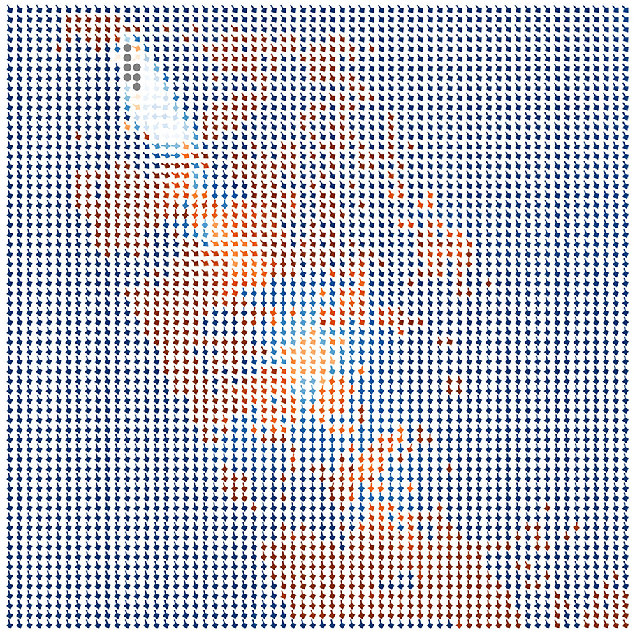
Figure 7. Reconstructed real-world sample. The red arrows indicate the known data points, the blue arrows show the reconstructed data points, and the brightness of the arrows encodes the magnitudes.

Figure 8 shows the result of our model (center) and the result of the least squares (right) for the same example in Figure 7. The curvy pattern of the vortex street is visible in both results, but unlike the least squares method, our model is also capable of reconstructing the turbulent vortex-generating structure in close vicinity to the island. To evaluate whether the vortices are preserved by our model and the least squares method, we examine the vorticity of the results in Figure 9, while showing satellite observations of the clouds in the background to provide context. While there is, unfortunately, no ground truth velocity field available for such observational data, an agreement of vortex structures with the underlying cloud patterns gives a strong indication for correctness, since the reconstructed flow is able to explain the fluid dynamical processes leading to the observable patterns (Horváth et al., 2020). From left to right we show the vorticity of the original data, our reconstruction with the neural network, and the least squares result. It can be seen that our model gives superior results, preserving the position and size of the different vortices. The visualization of the flow magnitudes in Figure 10 underlines this, showing that our model (center) results in a more reliable reconstruction of the flow structure than the least squares solution (right).

FIGURE 8

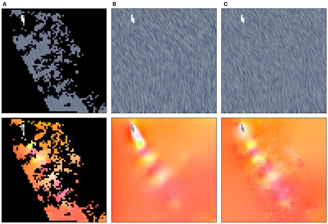
Figure 8. LIC and HSV visualization of the results obtained by reconstructing a real-world data sample (A) with our model (B) and with a least squares method (C).

FIGURE 9

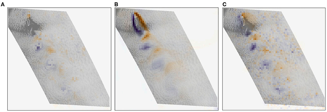
Figure 9. Vorticity visualization of the smoothed real-world data sample (A), the reconstruction with our neural method (B), and the least squares method (C).

FIGURE 10

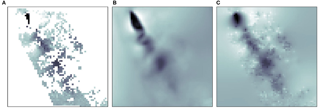
Figure 10. Magnitude visualization of the smoothed real-world data sample (A), our reconstruction (B), and the least squares solution (C).

4. Conclusions

Satellite-based wind retrieval enables a high-resolution view onto atmospheric air flows. This data, however, is intrinsically noisy, which is usually addressed through median filters or spatial smoothing. In this paper, we regularized the reconstruction from partial and noisy data in a data-driven approach using a U-Net based convolutional neural network. Based on model simulations, we generated training data to teach a neural network to disambiguate the partial observations based on physically-realizable flow configurations that have been observed during training. Our results on the synthetic flow data sets demonstrate that the use of neural networks can be successfully applied to flow data recovery tasks. Our case study on the Guadalupe Island data set demonstrates the practical impact of this physics-aware neural network on data post-processing, evaluation, and prediction in atmospheric modeling. The proposed neural-based method is especially powerful in high-occlusion applications, where the least squares method fails to provide reliable results. We further found that dilated convolution increases the number of data points used by the model to predict larger areas of missing data. This leads to better high-resolution results and prevents poor predictions – it can even be helpful in medium-resolution data sets without obstacles.

A neural network can only handle what it has seen during training. For extreme events, such as storms or floods, our currently trained model is likely to fail. The next step would be to study from observational or long-term reanalysis data the different boundary conditions that would occur in extreme events, and to then sample those conditions to initialize our ground truth simulations. It will then be important to create a training data set that is evenly balanced in its different flow configurations, such that extreme events are not too rare in the training data.

For the Guadalupe flow, unfortunately, no ground truth vector field is available, since this is a measured vector field. Instead, plausibility is usually tested by considering the spatial coherence of wind vectors (cf. Horváth et al., 2020). Additionally, Horváth et al. (2020) derived vortex measures assuming that a good agreement of vortex locations and visible cloud patterns is an indicator for a reasonable wind vector field that can explain the fluid dynamical processes that are visible in observations, which is also the approach we took in this manuscript. Determining additional validation heuristics is an interesting avenue in itself, which is beyond the scope of this paper.

Considering subsequent data points in time could potentially improve our model and allow for spatio-temporal reconstructions of flow structures. We found that when reconstructing each frame of the Guadalupe island sequence individually, the neural network prediction is smooth in most areas except the one in close vicinity to the island. This is because turbulent flow structures emerge in those regions, which cannot be captured coherently in time by a single-frame reconstruction technique.

Our model could also be used to determine the data points that give our model the least information (the best data points to mask) by calculating the gradient for the mask and not for the input. It could further inspire new techniques for compressing meteorological data and hence reducing data storage. Beyond meteorological applications, the method could impact related fields as well, such as finding optimal guiding procedures for human-based flow scanning systems, or improved workflows for digital prototyping where quick flow previews are particularly useful.

When surface altimetry data is available, for example from SWOT (surface water and ocean topography) missions, it could be added as additional channel to the network, allowing the network to pick up information that helps to disambiguate the partial observations further. Studying its effect would be another interesting avenue for future research.

Data Availability Statement

The raw data supporting the conclusions of this article will be made available by the authors, without undue reservation.

Author Contributions

LS, SF, and VA carried out the implementation and performed the calculations. LS, SF, JT, VA, TG, and BS developed the theoretical formalism and wrote the manuscript. JT, VA, TG, and BS supervised the project and conceived the original idea. All authors contributed to the article and approved the submitted version.

Funding

This work was supported by the Swiss National Science Foundation under Grant number CRSK-2_190296.

Conflict of Interest

The authors declare that the research was conducted in the absence of any commercial or financial relationships that could be construed as a potential conflict of interest.

References

Baño-Medina, J. L., García Manzanas, R., and Gutiérrez Llorente, J. M. (2020). Configuration and intercomparison of deep learning neural models for statistical downscaling. Geosci. Model Dev. 13, 2109–2124. doi: 10.5194/gmd-2019-278

CrossRef Full Text | Google Scholar

Brunton, S. L., Noack, B. R., and Koumoutsakos, P. (2020). Machine learning for fluid mechanics. Annua. Rev. Fluid Mech. 52, 477–508. doi: 10.1146/annurev-fluid-010719-060214

CrossRef Full Text | Google Scholar

Carr, J. L., Wu, D. L., Wolfe, R. E., Madani, H., Lin, G. G., and Tan, B. (2019). Joint 3D-wind retrievals with stereoscopic views from MODIS and GOES. Rem. Sens. 11:2100. doi: 10.3390/rs11182100

CrossRef Full Text | Google Scholar

Chopra, K. P., and Hubert, L. F. (1965). Mesoscale eddies in wake of islands. J. Atmos. Sci. 22, 652–657. doi: 10.1175/1520-0469(1965)022<0652:MEIWOI>2.0.CO;2

CrossRef Full Text | Google Scholar

Choy, C. B., Xu, D., Gwak, J., Chen, K., and Savarese, S. (2016). “3D-R2N2: a unified approach for single and multi-view 3D object reconstruction,” in Computer Vision–ECCV 2016 (Amsterdam), 628–644. doi: 10.1007/978-3-319-46484-8_38

CrossRef Full Text | Google Scholar

Geerts, B., Raymond, D. J., Grubisic, V., Davis, C. A., Barth, M. C., Detwiler, A., et al. (2018). Recommendations for in situ and remote sensing capabilities in atmospheric convection and turbulence. Bull. Am. Meteorol. Soc. 99, 2463–2470. doi: 10.1175/BAMS-D-17-0310.1

CrossRef Full Text | Google Scholar

Goodfellow, I., Pouget-Abadie, J., Mirza, M., Xu, B., Warde-Farley, D., Ozair, S., et al. (2014). “Generative adversarial nets,” in Advances in Neural Information Processing Systems, eds Z. Ghahramani, M. Welling, C. Cortes, N. Lawrence, and K. Q. Weinberger (Montreal, QC: Curran Associates, Inc.), 2672–2680.

Google Scholar

Guo, Y., and Tong, X. (2018). “View-volume network for semantic scene completion from a single depth image,” in IJCAI'18: Proceedings of the 27th International Joint Conference on Artificial Intelligence (Stockholm), 726–732. doi: 10.24963/ijcai.2018/101

CrossRef Full Text | Google Scholar

Han, X., Zhang, Z., Du, D., Yang, M., Yu, J., Pan, P., et al. (2019). “Deep reinforcement learning of volume-guided progressive view inpainting for 3D point scene completion from a single depth image,” in 2019 IEEE/CVF Conference on Computer Vision and Pattern Recognition (CVPR) (Long Beach, CA). doi: 10.1109/CVPR.2019.00032

CrossRef Full Text | Google Scholar

Hersbach, H., Bell, B., Berrisford, P., Hirahara, S., Horányi, A., Muñoz-Sabater, J., et al. (2020). The ERA5 global reanalysis. Q. J. R. Meteorol. Soc. 146, 1999–2049. doi: 10.1002/qj.3803

CrossRef Full Text | Google Scholar

Horváth, Á., Bresky, W., Daniels, J., Vogelzang, J., Stoffelen, A., Carr, J. L., et al. (2020). Evolution of an atmospheric Kármán vortex street from high-resolution satellite winds: Guadalupe island case study. J. Geophys. Res. Atmos. 125:e2019JD032121. doi: 10.1029/2019JD032121

CrossRef Full Text | Google Scholar

Horváth, Á., Hautecoeur, O., Borde, R., Deneke, H., and Buehler, S. A. (2017). Evaluation of the eumetsat global avhrr wind product. J. Appl. Meteorol. Climatol. 56, 2353–2376. doi: 10.1175/JAMC-D-17-0059.1

CrossRef Full Text | Google Scholar

Huang, G., Liu, Z., Van Der Maaten, L., and Weinberger, K. Q. (2017). “Densely connected convolutional networks,” in Proceedings–30th IEEE Conference on Computer Vision and Pattern Recognition, CVPR 2017 (Honolulu), 2261–2269. doi: 10.1109/CVPR.2017.243

CrossRef Full Text

Hubert, L. F., and Krueger, A. F. (1962). Satellite pictures of mesoscale eddies. Mon. Weather Rev. 90, 457–463. doi: 10.1175/1520-0493(1962)090<0457:SPOME>2.0.CO;2

CrossRef Full Text | Google Scholar

Iizuka, S., Simo-Serra, E., and Ishikawa, H. (2017). Globally and locally consistent image completion. ACM Trans. Graph. 36:107. doi: 10.1145/3072959.3073659

CrossRef Full Text | Google Scholar

Kim, B., Azevedo, V., Gross, M., and Solenthaler, B. (2019a). Transport-based neural style transfer for smoke simulations. ACM Trans. Graph. 38, 188:1–188:11. doi: 10.1145/3355089.3356560

CrossRef Full Text | Google Scholar

Kim, B., Azevedo, V. C., Thuerey, N., Kim, T., Gross, M., and Solenthaler, B. (2019b). Deep fluids: a generative network for parameterized fluid simulations. Comput. Graph. Forum 38, 59–70. doi: 10.1111/cgf.13619

CrossRef Full Text | Google Scholar

Liu, G., Reda, F. A., Shih, K. J., Wang, T. C., Tao, A., and Catanzaro, B. (2018). Image inpainting for irregular holes using partial convolutions. Lect. Notes Comput. Sci. 11215, 89–105. doi: 10.1007/978-3-030-01252-6_6

CrossRef Full Text | Google Scholar

Min, M., Li, J., Wang, F., Liu, Z., and Menzel, W. P. (2020). Retrieval of cloud top properties from advanced geostationary satellite imager measurements based on machine learning algorithms. Rem. Sens. Environ. 239:111616. doi: 10.1016/j.rse.2019.111616

CrossRef Full Text | Google Scholar

O'Gorman, P. A., and Dwyer, J. G. (2018). Using machine learning to parameterize moist convection: potential for modeling of climate, climate change, and extreme events. J. Adv. Model. Earth Syst. 10, 2548–2563. doi: 10.1029/2018MS001351

CrossRef Full Text | Google Scholar

Pathak, D., Krahenbuhl, P., Donahue, J., Darrell, T., and Efros, A. A. (2016). “Context encoders: feature learning by inpainting,” in Proceedings of the IEEE Computer Society Conference on Computer Vision and Pattern Recognition (Las Vegas, NV), 2536–2544. doi: 10.1109/CVPR.2016.278

CrossRef Full Text | Google Scholar

Raissi, M., Yazdani, A., and Karniadakis, G. E. (2018). Hidden fluid mechanics: a navier-stokes informed deep learning framework for assimilating flow visualization data. arXiv [Preprint]. arXiv:1808.04327.

Google Scholar

Ronneberger, O., Fischer, P., and Brox, T. (2015). U-net: convolutional networks for biomedical image segmentation. Lect. Notes Comput. Sci. 9351, 234–241. doi: 10.1007/978-3-319-24574-4_28

CrossRef Full Text | Google Scholar

Schmit, T. J., Griffith, P., Gunshor, M. M., Daniels, J. M., Goodman, S. J., and Lebair, W. J. (2017). A closer look at the abi on the goes-R series. Bull. Am. Meteorol. Soc. 98, 681–698. doi: 10.1175/BAMS-D-15-00230.1

CrossRef Full Text | Google Scholar

Seifert, A., and Rasp, S. (2020). Potential and limitations of machine learning for modeling warm-rain cloud microphysical processes. J. Adv. Model. Earth Syst. 12:e2020MS002301. doi: 10.1029/2020MS002301

CrossRef Full Text | Google Scholar

Song, S., Yu, F., Zeng, A., Chang, A., Savva, M., and Funkhouser, T. (2017). “Semantic scene completion from a single depth image,” in 2017 IEEE Conference on Computer Vision and Pattern Recognition (CVPR) (Honolulu) 190–198. doi: 10.1109/CVPR.2017.28

CrossRef Full Text | Google Scholar

Thuerey, N., and Pfaff, T. (2018). MantaFlow. Available online at: http://mantaflow.com

Umetani, N., and Bickel, B. (2018). Learning three-dimensional flow for interactive aerodynamic design. ACM Trans. Graph. 37, 89:1–89:10. doi: 10.1145/3197517.3201325

CrossRef Full Text | Google Scholar

Weyn, J. A., Durran, D. R., and Caruana, R. (2019). Can machines learn to predict weather? Using deep learning to predict gridded 500-HPA geopotential height from historical weather data. J. Adv. Model. Earth Syst. 11, 2680–2693. doi: 10.1029/2019MS001705

CrossRef Full Text | Google Scholar

Wiewel, S., Becher, M., and Thuerey, N. (2019). Latent-space physics: towards learning the temporal evolution of fluid flow. Comput. Graph. Forum 38, 71–82. doi: 10.1111/cgf.13620

CrossRef Full Text | Google Scholar

Xu, K., Shi, Y., Zheng, L., Zhang, J., Liu, M., Huang, H., et al. (2016). 3D attention-driven depth acquisition for object identification. ACM Trans. Graph. 35, 238:1–238:14. doi: 10.1145/2980179.2980224

CrossRef Full Text | Google Scholar

Young, G. S., and Zawislak, J. (2006). An observational study of vortex spacing in island wake vortex streets. Mon. Weather Rev. 134, 2285–2294. doi: 10.1175/MWR3186.1

CrossRef Full Text | Google Scholar

Yu, J., Lin, Z., Yang, J., Shen, X., Lu, X., and Huang, T. S. (2018). “Free-form image inpainting with gated convolution,” in IEEE/CVF International Conference on Computer Vision (ICCV) (Istanbul), 4470–4479. doi: 10.1109/ICCV.2019.00457

CrossRef Full Text | Google Scholar

Zeng, Y., Fu, J., Chao, H., and Guo, B. (2019). “Learning pyramid-context encoder network for high-quality image inpainting,” in 2019 IEEE/CVF Conference on Computer Vision and Pattern Recognition (CVPR) (Long Beach, CA), 1486–1494. doi: 10.1109/CVPR.2019.00158

CrossRef Full Text | Google Scholar

Zhang, Y., and Funkhouser, T. A. (2018). “Deep depth completion of a single RGB-D image,” in IEEE Conference on Computer Vision and Pattern Recognition (Salt Lake City, UT), 175–185. doi: 10.1109/CVPR.2018.00026

CrossRef Full Text | Google Scholar

Appendix

Network Architectures

We specify the network architectures in Tables A1–A4. All layers in the encoder, dense block and decoder are Partial Convolution layers described in Equation (1). The layers in the stream function branch are normal convolutional layers. Batch normalization is used for all layers except the output layer and layers in the stream function branch. We use ReLU activation functions for layers in the encoder and dense block, LeakyReLU activation function for layers in the decoder and Swish activation function for the stream function branch. The output of the stream function branch is used to compute the velocity field: ${\widehat{\overrightarrow{u}}}_{\psi }=(\frac{\partial \psi }{\partial y},-\frac{\partial \psi }{\partial x})$. Then, ${\widehat{\overrightarrow{u}}}_{\psi }$ is concatenated with the output from the velocity branch and goes through a normal convolutional layer to produce the final velocity prediction $\widehat{\overrightarrow{u}}$.

TABLE A1

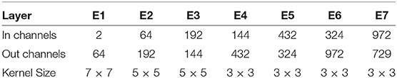
Table A1. Network layer configurations of the encoder part.

TABLE A2

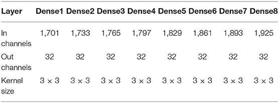
Table A2. Network layer configurations of the DenseBlock part.

TABLE A3

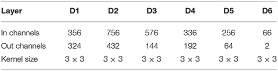
Table A3. Network layer configurations of the decoder part.

TABLE A4

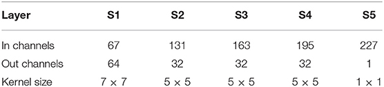
Table A4. Network layer configurations of the stream function branch.

Training Details

All models were trained with Adam optimizer with β₁ = 0.9 and β₂ = 0.999, and the learning rate was set to 10⁻⁵. We used a batch size of 8 and train all models for 50 epochs.