Week 3–4 Prediction of Wintertime CONUS Temperature Using Machine Learning Techniques

1. Introduction

This paper concerns predictions out to weeks 3–4. Such predictions differ from weather forecasts (i.e., predicting individual days) in that they forecast the mean over a 2-week period instead of individual days. In this sense, week 3–4 forecasts are similar to seasonal forecasts in that both involve predicting the mean weather over an interval longer than a week.

Several predictors have been identified as having the potential to be a source of predictability in a week 3–4 forecast. A dominant source of predictability (especially in winter) are the ocean-atmosphere interactions, especially the effects of ENSO and the Madden-Julian oscillation (MJO) (e.g., Shukla and Kinter, 2006). These tropical phenomena are associated with anomalous convective heating in the atmosphere, which excites Rossby waves that can influence weather over North America. Alternatively, in the winter sudden stratospheric warming events can cause anomalous temperatures throughout the atmosphere that last for weeks. At the surface, this temperature signal can persist for up to a month (Baldwin et al., 2021). Snow cover and the top meter of soil moisture last for weeks after precipitation events and can be a source of influence for temperature and precipitation over those weeks (e.g., Sobolowski et al., 2007; Guo et al., 2011). Individual high impact events such as volcanic eruptions, while much rarer, can also provide a source of long lasting predictability (National Research Council, 2010). Not all of these variables will necessarily be able to be used in all places or at all times, but many of them might be able to be a source of predictability on week 2–8 time scales.

The Climate Prediction Center (CPC) currently issues an operational week 3–4 temperature forecast over the Contiguous United States (CONUS). This forecast is made from several sources, including forecasts made by SubX dynamical models (Pegion et al., 2019), forecaster experience, and a statistical model which is based in part on the phase of ENSO, the phase of the MJO, and the multi-decadal trend—all of which are calculated from 30 years of reanalysis data (Johnson et al., 2014).

By far the strongest source of sub-seasonal predictability over North America comes from Pacific sea surface temperatures (SSTs), particularly those associated with El Niño. In the 1970s and 1980s, SST indices (called Nino 1–4) were established to represent the state of El Niño. These indices were chosen at least in part by convenience—these areas corresponded with common ship routes and arrays of observational buoys such as the TAO array (McPhaden et al., 2010) where SST data was readily available. In the late 1990s, the Nino3.4 index was identified as being the most representative of ENSO as a whole (Barnston et al., 1997). While regression predictions based on the Nino3.4 index can make skillful subseasonal forecasts over CONUS, this is not necessarily the index that optimizes these forecasts.

Recently, NOAA partnered with the Bureau of Reclamation to run public forecast competitions in 2016 and again in 2019 (see https://www.usbr.gov/research/challenges/forecastrodeo.html). The winner of the 2016 competition (Hwang et al., 2019) used machine learning with predictors taken from observations of a number of variables as well as long range forecasts made by the North American Multi-Model Ensemble.

The goal of this paper is to see if there is another source of week 3–4 predictability from SSTs or a better tropical Pacific index which can optimally capture subseasonal predictability. We will be using only SST data as predictors, so we expect to find the largest signal to be from ENSO. However, because we are not limiting our prediction to the ENSO indices, we hope to be able to find more than what the ENSO indices alone can tell us.

To identify better predictors, we used machine learning techniques called lasso and ridge regression. Ridge regression was originally designed to solve the problem of singular matrices caused by nearly collinear predictors. On the other hand, lasso was derived by Tibshirani (1996) to combine two features. The first is prediction accuracy. Lasso shrinks the predictors and sets some of them to exactly zero. Shrinkage is known to increase the skill of a prediction made with many predictors by reducing the variance of the prediction (Copas, 1983). The second feature is interpretation. Since lasso sets some predictors to exactly zero, that gives us the chance to interpret the remaining predictors.

In making a forecast for observations, we trained lasso and ridge regression on observational data and were able to make a prediction with some skill (see section 4). However, there is always the risk of overfitting and artificially increasing the skill of the prediction when training and predicting the same data set. An alternative approach that avoids this risk is to train on dynamical model data and then test on independent observations. This gives us a larger sample size and also allows us to test if dynamical models can capture predictive relations. The dynamical models that were used come from the Coupled Model Intercomparison Project Phase 5 (CMIP5) PreIndustrial Control runs. These runs are simulations where the external forcing (e.g., CO₂ levels, aerosols, or land use) is prescribed to be what they were in 1850 and persist for each year after that. PreIndustrial Control data is used both because of the abundance of models which produce this kind of control data and to avoid confounding trends produced by external forcing. Ridge regression and lasso would pick up on externally forced trends to make a prediction, but we are trying to make a prediction based on internal dynamics. While forecasting based on external forcing may be an interesting topic to explore, this paper is focusing on using only internal dynamics to make forecasts. Despite PreIndustrial Control runs being forced with the external forcing from 1850, it has been shown that changes 2 m temperature teleconnections due to external forcing are small (DelSole et al., 2014).

2. Data

2.1. Laplacian Eigenvectors

As discussed earlier, SST influences sub-seasonal temperature over CONUS primarily through Rossby wave teleconnection mechanisms. Such waves are well-established in midlatitudes after about 15 days of tropical heating (Jin and Hoskins, 1995). Furthermore, the structure of the midlatitude response is largely insensitive to the longitudinal position of the heating anomaly (Geisler et al., 1985). As a result, the predictable relation between SST and midlatitude temperature is anticipated to be characterized by only a few large-scale patterns. Therefore, instead of individual grid points, we predict large-scale spatial structures of CONUS 2 m temperature. A convenient set of large-scale patterns are provided by the eigenvectors of the Laplace operator, called Laplacians in this paper. Laplacians are an orthogonal set of patterns ordered by spatial length scale. On a sphere, Laplacians are merely the well-known spherical harmonics. For the CONUS domain, we use the algorithm of DelSole and Tippett (2015) to derive the Laplacians. The first few Laplacians over CONUS is shown in Figure 1. Because the predictable space is anticipated to be low-dimensional, not all of the Laplacian eigenvectors are anticipated to be predictable. We predicted each of the Laplacians separately and found that only the third CONUS Laplacian could be predicted skillfully. This result is consistent with the fact that this Laplacian projects strongly onto the ENSO signal over CONUS (e.g., Higgins et al., 2004) and looks like the most predictable pattern in the dynamical model CFSv2, which is shown in Figure 8 of DelSole et al. (2017). For these reasons, the 3rd Laplacian eigenfunction is referred to as the “ENSO-forced temperature pattern,” and the projection of 2 m temperature on this pattern is the predictand in this study. The ENSO-forced temperature pattern represents 12.4% of the variance of the 2-week mean 2 m Temperature anomalies over CONUS. Although the Laplacians are large scale, individual patterns are not necessarily associated with definite climate signals. Incidentally, it is entirely possible that using predictors other than SSTs could lead to a different Laplacian being predictable, or multiple predictable Laplacians.

FIGURE 1

Figure 1. Laplacian eigenvectors 2–7 over CONUS. The first Laplacian eigenvector is not shown as that is simply the spatial average over the domain.

2.2. Data

The observational data used in this study is daily 2 m temperature as well as observed daily SSTs produced by the CPC for the period 1981 to 2018. Both data sets are provided by the Earth Systems Research Laboratory Physical Sciences Division (ESRL PSD), Boulder, Colorado, USA and are available on their website (https://www.esrl.noaa.gov/psd/). The domain of interest for 2 m temperature is land points within 25° to 50°N and 125° to 67°W, which, although not exactly CONUS, is referred to as CONUS in the remainder of this paper. Two SST domains were considered for this study—the Tropical Pacific (25°S to 25°N and 125°E to 60°W) and the Atlantic plus Pacific (30°S to 60°N and 125°E to 8°W).

We also used SSTs from 18 CMIP5 models with PreIndustrial Control forcing to train the machine learning algorithms. We included a model only if it had at least 100 years of daily data output. See Table 1 for the list of the models used as well as the length of each model run.

TABLE 1

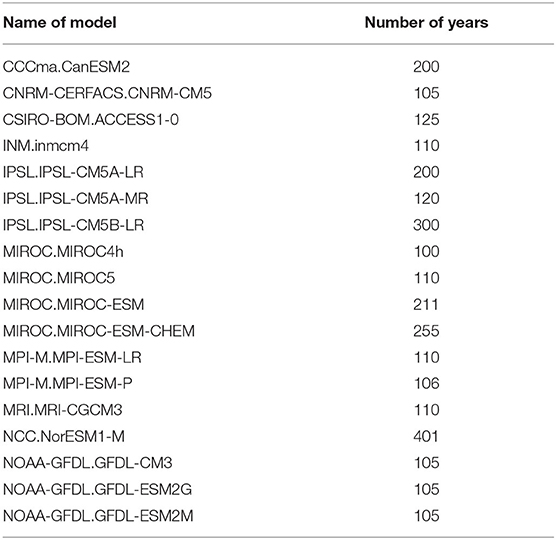
Table 1. List of the CMIP5 models used and the corresponding length of the daily dataset, in years.

Since our goal is to find a better predictor than the Nino3.4 index, we choose a region much larger than the Nino3.4 region and let the optimization algorithm choose the best predictors. If the chosen domain is “too large” and a more localized domain is better, then lasso/ridge regression has the flexibility to choose grid points in just that domain.

2.3. Pre-processing

The 2 m Temperature data was interpolated onto a 2.5 × 2.5 degree grid and projected onto the third CONUS Laplacian (see section 2.1) and the SST data onto a 4 × 4 degree grid. In order to account for the seasonal cycle, the first three annual harmonics of daily means were regressed out of each data set. To account for any trends, a third-degree polynomial was regressed out of each data set. Finally, the predictors (SSTs) were normalized such that the sum of the variance of all of the predictors equals 1 and the CONUS predictand was normalized to unit variance in time. This was done in order to minimize the effect of amplitude errors across dynamical models when making a prediction. Observations and CMIP5 dynamical model data were processed the same way.

2.4. Time Definitions

The predictand in this study is a 2 week mean of 2 m temperature anomalies over CONUS. The predictor is a 1 week mean of sea surface temperature anomalies (SST), which ends 2 weeks before the 2 week period we want to predict begins. To put another way, if today is day 0, the SSTs were averaged from day −7 to day 0 to construct the initial condition, and then we predict the average of day 14 through day 28 CONUS temperature. SSTs evolve on a much slower time scale than the atmosphere, so there is almost no difference between a 1-week and 2-week average. Also, our target is 2-week means, so averaging longer than 2 weeks would prevent us from capturing predictability that varies between 2-week means. The time period examined is boreal winter, defined as predictions made in December, January, and February (DJF).

2.5. Nino3.4 Index

The Nino3.4 index is defined as the average of the region bounded by 5°N to 5°S, and from 170 to 120°W. The annual cycle and trends were removed from the Nino3.4 index in the same way as the rest of the data, described in section 2.3, and averaging in time described in section 2.4. To calculate the regression coefficient for the Nino3.4 index we used leave 1 year out ordinary least squares. That is, one winter of data was left out, and from the remaining data the regression coefficient for that year was calculated using ordinary least squares.

2.6. Dynamical Model Data - CFSv2

The question arises of how our machine learning method compares to a dynamical model. To answer this question we compared the skill of machine learning models to the skill of a fully coupled dynamical model. The model we chose was the NCEP CFSv2 model, an operational forecast model and a contributing member of the SubX dataset (Pegion et al., 2019). The SubX data is freely available on their website (http://iridl.ldeo.columbia.edu/SOURCES/.Models/.SubX/). The hindcast is available from January 1, 1999 to December 31, 2015. The hindcast is initialized daily, and each initialization is run for 45 days. Anomalies of the hindcast are precomputed, with the climatology calculated as a function of lead time and initialization date, as described in Appendix B of Pegion et al. (2019). To calculate the skill of this model, we projected the forecasts of 2 m temperature onto the Laplacians (described in section 2.1), averaged over weeks 3–4 for each prediction made in DJF, corrected amplitude errors by using leave 1 year out ordinary least squares, and calculated the Mean Squared Error (described in section 3.2) and correlation skill relative to the observations (described in section 2.2).

3. Methods

3.1. Machine Learning Technique - Lasso and Ridge Regression

Our prediction equation is

$\begin{array}{ll}{ŷ}_f={\displaystyle \sum _{p=1}^P}{x}_{fp}{\beta }_p+{\beta }_0,\text{ for}\mathrm{ f}=1,2,\dots F& (1)\end{array}$

where ŷ_f is the forecasted (anomalous) time series of the ENSO-forced temperature pattern (i.e., the 3rd Laplacian eigenvector over CONUS) at the f^th forecast, x_fp is the time series of the p^th SST grid point at the f^th forecast, β_p is a weighting coefficient connecting the p^th SST grid point's time series to the ENSO-forced temperature pattern, and β₀ is the intercept term. The set of β_p is referred to as “beta coefficients” in the remainder of this paper.

To estimate β in Equation (1), we used machine learning algorithms called lasso and ridge regression. For an excellent description of lasso and ridge regression and their differences, we recommend the textbook by Hastie et al. (2009). Lasso minimizes the equation

$\begin{array}{ll}{\displaystyle \sum _{f=1}^F}{(y_f-{ŷ}_f)}^2+\lambda {\displaystyle \sum _{p=1}^P}|{\beta }_p|.& (2)\end{array}$

Similarly, ridge regression minimizes the equation

$\begin{array}{ll}{\displaystyle \sum _{f=1}^F}{(y_f-{ŷ}_f)}^2+\lambda {\displaystyle \sum _{p=1}^P}{\beta }_p{}^2.& (3)\end{array}$

In both cases the variables are the same as Equation (1), F is the number of forecasts, P is the number of predictors, y_f is the true time series of the ENSO-forced temperature pattern at the f^th forecast and λ is an adjustable parameter. β_p is embedded in ŷ_f. β₀ is not included in the summation in the second term of Equations (2) and (3).

The result of using either technique is a set of βs as a function of λ. There is a question of model selection—which λ do we choose? A standard method of choosing λ will be presented; however this standard method is not optimal in this study and we adjusted the method slightly to better fit with the rest of our method. This will be presented in section 3.5.

One of lasso's properties that we hope will be useful for interpretation is that at sufficiently large λ all of the βs will be exactly zero, while at sufficiently small λ β will converge to the Ordinary Least Squares solution for β. In between, some of the βs will be exactly zero. One way to interpret this is that those predictors associated with the zero βs are not as important as the other predictors when making a prediction. So we might be able to “pick out” the most important 3 or 4 predictors for our prediction. One caveat is that if several predictors are strongly correlated, lasso will only pick a few predictors and will set the coefficients of the remaining predictors to zero. This could lead to a strong sample dependence in the selection of predictors.

Ridge regression, unlike lasso, does not set the coefficients of any predictors to zero—all predictors are included. If several predictors are strongly correlated with each other, all of those predictors are selected but with a smaller amplitude than the amplitude of the one predictor that would be selected by lasso. This can make interpretation much more difficult for Ridge regression.

3.2. Measure of Skill - Normalized Mean Squared Error

To measure the skill in predicting the ENSO-forced temperature pattern, the Normalized Mean Squared Error (NMSE) is calculated as

$\begin{array}{ll}NMSE(\lambda )=\frac{{\displaystyle {\sum }_{f=1}^F{\left(y_f-{\widehat{y}}_f\right)}^2}}{{\displaystyle {\sum }_{f=1}^F{\left(y_f-\overline{y}\right)}^2}},& (4)\end{array}$

where the variables are the same as in Equations (1)–(3) and ȳ is the climatological mean temperature over the period in question. A Normalized Mean Squared Error of less than 1 means that the statistical model is a better prediction than the climatological mean, while a Normalized Mean Squared Error of greater than 1 means that it is worse than a prediction based on the climatological mean. Normalizing by the climatological mean offers a standard model-independent measure of comparison. Because the βs are a function of λ the NMSE is likewise evaluated over that range of λ. Since NMSE penalizes amplitude errors, we consider an alternative skill measure based on the anomaly correlation (also called the cosine-similarity):

$\begin{array}{ll}cor(\lambda )=\frac{{\displaystyle {\sum }_{f=1}^F(y_f-\overline{y})({\widehat{y}}_f-\overline{\widehat{y}})}}{\sqrt{{\displaystyle {\sum }_{f=1}^F{(y_f-\overline{y})}^2}}\sqrt{{\displaystyle {\sum }_{f=1}^F{({\widehat{y}}_f-\overline{\widehat{y}})}^2}}},& (5)\end{array}$

where all variables are the same as in Equation (4) and $\overline{ŷ}$ is the mean predicted temperature.

Not only are we are trying to make predictions which are better than climatology, we are trying to improve on the current state of subseasonal predictions. Although the details differ somewhat, the Climate Prediction Center uses the Nino3.4 index as part of their statistical guidance when making a week 3–4 or week 5–6 forecast (Johnson et al., 2014). We are trying to see if there is a better index for making predictions of CONUS compared to the standard Nino3.4 index. To find the skill of the Nino3.4 index, we calculated its NMSE following Equation (4), where x is the observed time series of the index and β was calculated using leave 1 year out ordinary least squares.

3.3. NMSE Confidence Intervals - Bootstrap Test

To test whether the NMSE from a particular prediction model is significantly different from a prediction based on climatology (which has a NMSE of 1) we used the bootstrap test. To perform this test, we randomly sampled the errors of the 37 winters with replacements. We do this 10,000 times to estimate the distribution of the errors. The 5th and 95th percentiles of the distribution are the confidence intervals at the 5% level. If these confidence intervals do not include 1, then the prediction is significantly different from a prediction based on climatology. Because predictions made by ridge and lasso are potentially very different, each prediction is tested individually.

3.4. Cross Model and Multi-Model Comparison

Because the SST grid is the same across all regression models, the βs calculated from one data set can be used to make a prediction in another. In particular, because we are interested in predicting observations, we can use the βs estimated from the CMIP5 models to predict observations. Rewriting Equation (4) to reflect this gives a Normalized Mean Squared Error equation of:

$\begin{array}{ll}NMSE(\lambda )=\frac{{\displaystyle {\sum }_{f=1}^F\left(y_{f,obs}-{\displaystyle {\sum }_{p=1}^P\left(x_{fp,obs}{\beta }_{p,model}\right)}\right)}}{{\displaystyle {\sum }_{f=1}^F{\left(y_{f,obs}-{\overline{y}}_{obs}\right)}^2}},& (6)\end{array}$

where the variables are as in Equation (4) except that the βs are now calculated from the dynamical models instead of from observations. Subscripts indicate that x and y are the observed SSTs and CONUS temperatures, respectively.

Doing this allows us to make a prediction without worrying about overfitting because the prediction is made on a data set which is completely independent from observations. If a prediction was trained on observations and then also validated in observations, there would be some worry about overfitting due to using the data twice.

Given the success of ensembles in forecasting (e.g., Slater et al., 2019) and the number of different dynamical models that we used, we might want to consider a way to use all of the model data at once. There are several ways to do this, but we simply concatenated the time series of each of the dynamical models and let lasso find the βs of that time series. Then the Normalized Mean Squared Error is calculated as in Equation (6), where β_{p, model} refers to the βs calculated in this way. In the rest of the paper, a prediction made in this way is referred to as the multi-model prediction.

3.5. Choosing λ

Because the NMSE is a function of λ, we need a criterion for choosing λ. The standard method of choosing the λ is to perform a 10-fold cross-validation on the whole data set which produced β (Hastie et al., 2009). This is designed to give an estimate of the out-of-sample error. In our case, the data set that produced β (model data) is completely independent from the data set that we want to evaluate (observations). However, the machine learning models trained on climate model simulations are completely independent of observations, so a different selection criterion is needed. Here, we simply leave 1 year out, calculate NMSE as a function of lambda, and then select the lambda for that year using the “one standard error rule” discussed in section 7 of Hastie et al. (2009). After the lambda is selected for each year, a prediction is made based on that corresponding betas and the NMSE is computed over the 37-year predictions. This means that each year could have a different λ selected. Practically, however, there is little difference in the λ from year to year, so the prediction models for each year are almost identical.

Both the machine learning predictions and the Nino3.4 index involve a parameter that is estimated by leaving out the same data (that is, both the machine learning λ and the Nino3.4 regression coefficient for each winter were estimated by leaving out that winter and using the rest of the data for the calculation). Because of this, comparing the machine learning prediction to the Nino3.4 prediction will be as fair as possible—if there is an extreme anomaly in 1 year neither prediction method should have an advantage based on their coefficient selection.

3.6. Measure of Skill - Random Walk Test

We are interested in improving predictions, but comparisons based on NMSE or correlations have low statistical power, as discussed in DelSole and Tippett (2014). This low power means that it will be very difficult to identify statistically better forecasts merely by comparing NMSE or correlation. Accordingly, we apply a more powerful test. Specifically, we use the Random Walk test of DelSole and Tippett (2016). To do this test, we simply have to count the number of times our selected model has smaller squared error than a forecast based on the Nino3.4 index. To avoid serial correlations, we count only those forecasts starting on the same calendar day, so each forecast included in the count are separated by at least 1 year. For example, of the 37 forecasts made on January 1, we count how many of our forecasts had a smaller NMSE than the forecasts from the Nino3.4 index made on January 1, likewise for January 2 and so on. The resulting percentages are then plotted as a function of the calendar day of the initial condition. The 95% confidence intervals for each point are based on the binomial distribution and are exact for each particular date.

Looking at all 90 points at once might give us an idea of when in the winter the machine learning can make a better forecast than the Nino3.4 index. Although the forecasts that are made on a particular date are independent, the 37 forecasts made on January 1, for example, will be highly correlated with the 37 forecasts made on January 2. Due to this serial correlation the 95% confidence intervals will underestimate the uncertainty of this analysis. However, it may still give us a good idea of when the machine learning model is able to improve upon the Nino3.4 index and when it cannot.

4. Results

4.1. Tropical Pacific, Grid Point Predictors

The Nino3.4 index has a NMSE of 0.889 when predicting the third Laplacian of CONUS 2 m temperature. While we do define skillful to be better than climatology, since the Nino3.4 index has lower error than climatology, our real bar is Nino3.4.

The skill of predicting the ENSO-forced temperature pattern at weeks 3–4 using various regression models is shown in Figure 2A. As can be seen, ordinary regression based on the Nino3.4 index outperforms the machine learning techniques trained on observations. In fact, predictions made when observations are used to train the machine learning are not even significantly better than a prediction based on climatology. Training the machine learning techniques on long CMIP5 model simulations is significantly better than a prediction based on climatology, which suggests that while machine learning techniques can produce skillful predictions, the short sample size of the observations strongly limits their skill. Training on the CMIP5 model simulations has a slightly lower error than the prediction based on the Nino3.4 index. Whether this difference is statistically significant will be investigated shortly.

FIGURE 2

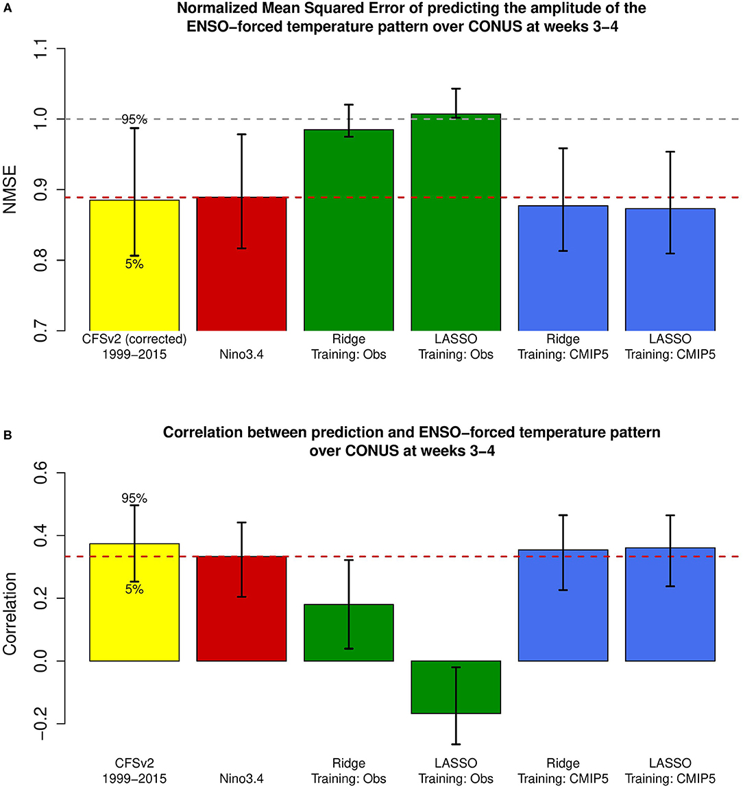
Figure 2. (A) Cross-validated normalized mean squared errors of predictions of the ENSO-forced temperature pattern, and (B) the associated correlation skills for the following models (from left to right): CFSv2 hindcast; ordinary least squares based on the Nino3.4 index; ridge regression trained on observed SST; lasso regression trained on observed SST; ridge regression trained on CMIP5 model simulations; lasso regression trained on CMIP5 model simulations. The validation time period for the CFSv2 hindcast is 1999–2015. The validation time period for the empirical models (right 5 bars) is 1981–2018. The empirical models only use tropical Pacific SST grid points as predictors. Error bars show the 5% and the 95% levels, calculated using a bootstrap method.

It is instructive to also compare the skill of the predictions made by machine learning with the skill of a fully coupled dynamical model. The NMSE of the CFSv2 dynamical model, presented as the first bar in Figure 2A, is actually slightly less skillful than the predictions made by the machine learning algorithms. This is likely due to amplitude errors, as the CFSv2 prediction has the largest correlation with the ENSO-forced temperature pattern (shown in Figure 2B), albeit by a relatively small margin.

To assess significance of differences in skill, we apply the random walk test described in section 3.6. Some representative results are shown in Figure 3. Some predictions are no better than a Nino3.4 index (Figure 4C), while others are significantly better than those based on Nino3.4 index, but only for short periods (Figures 4A,B). No prediction is significantly better than Nino3.4 for every calendar day. Accordingly, we say that some of the ML predictions are “modestly” better than predictions based on the Nino3.4 index.

FIGURE 3

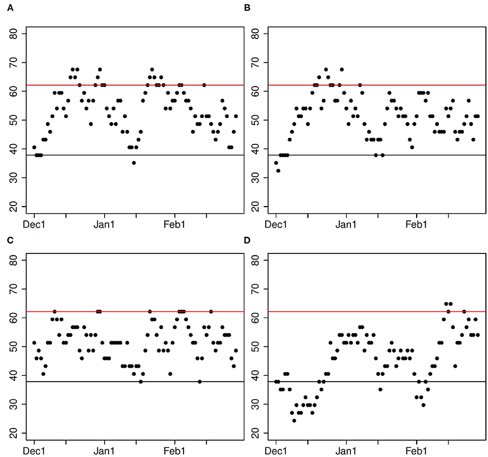
Figure 3. Percentage of times ML predictions are closer to observations than predictions using the Nino3.4 index. The percentage is plotted as a function of the calendar day of the initial condition. Only predictions starting on the same calendar day are used to calculate percentages. For each calendar day, there are 37 predictions, one for each of the 37 years. The different panels show results for the following predictions: (A) Tropical Pacific Laplacians using lasso, (B) Tropical Pacific grid points using ridge, (C) Tropical Pacific grid points using lasso, (D) Atlantic plus Pacific Laplacians using lasso. Points above the red line indicate initial conditions when a prediction made with machine learning is significantly better (at the 5% level) than a prediction made with the Nino3.4 index. Points below the black line indicate initial conditions when predictions made with the Nino3.4 index are significantly better than predictions from ML. Panels (A,B) are both moderate improvements on the Nino3.4 index, (C) is statistically indistinguishable from the Nino3.4 index, and (D) is significantly worse than the Nino3.4 index.

FIGURE 4

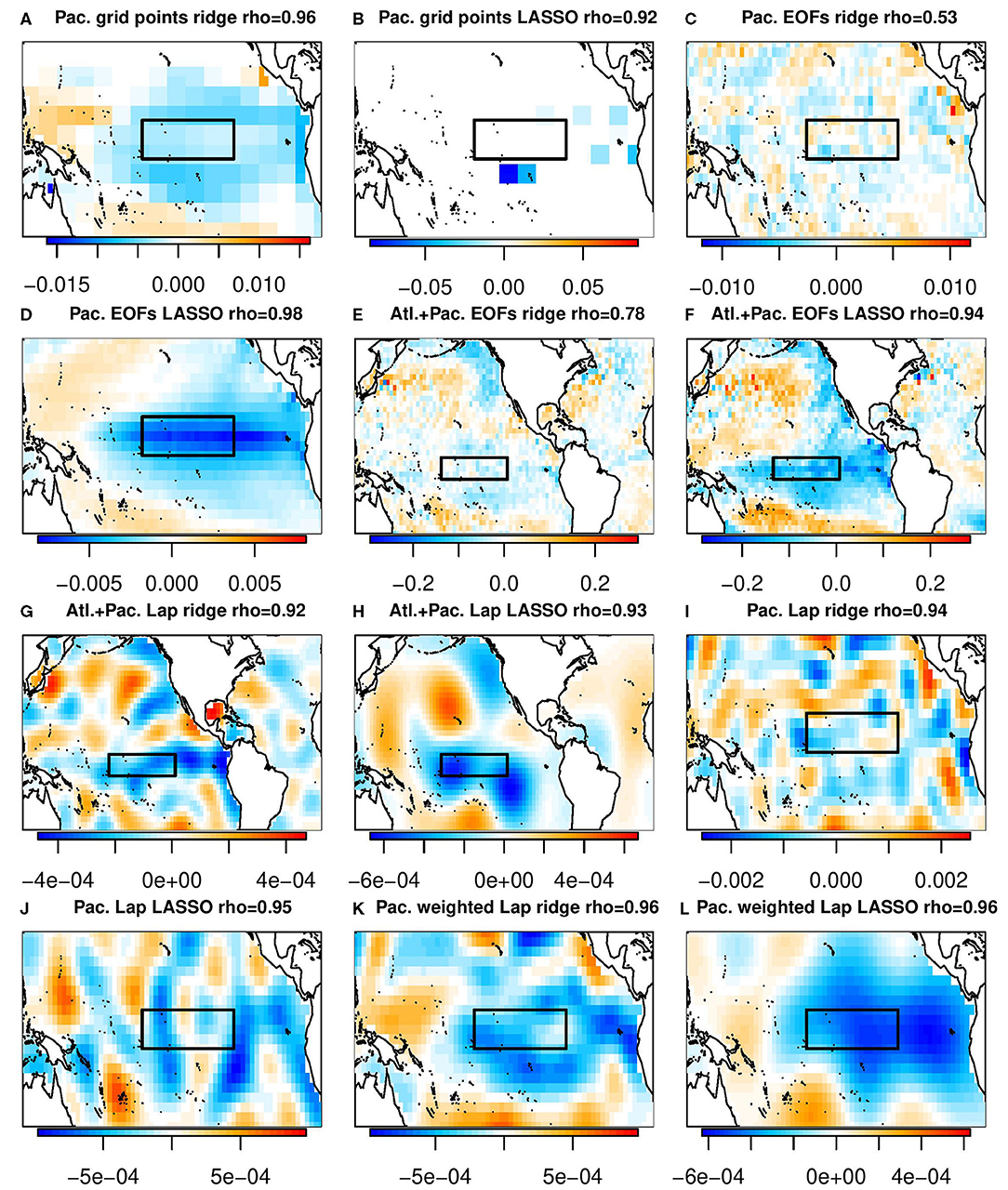
Figure 4. The β coefficients selected by various machine learning algorithms. Titles of the individual panels indicate the domain, basis set, machine learning algorithm used, and the correlation between the resulting prediction and the Nino3.4 index. The black boxes indicates the Nino3.4 index. (A) Pac. grid points ridge rho = 0.96. (B) Pac. grid points LASSO rho = 0.92. (C) Pac. EOFs ridge rho = 0.53. (D) Pac. EOFs LASSO rho = 0.98. (E) Alt+Pac. EOFs ridge rho = 0.78. (F) Alt+Pac. EOFs LASSO rho = 0.94. (G) Alt+Pac. Lap ridge rho = 0.92. (H) Alt+Pac. Lap LASSO rho = 0.93. (I) Pac. Lap ridge rho = 0.94. (J) Pac. Lap LASSO rho = 0.95. (K) Pac. weighted Lap ridge rho = 0.96. (L) Pac. weighted Lap LASSO rho = 0.96.

Figure 4 shows the β coefficients associated with the ridge regression prediction and the lasso prediction, respectively. As can be seen, the spatial maps can differ greatly. Nevertheless, they yield very similar predictions (e.g, the correlation with the Nino3.4 index exceeds 0.9 in most cases). This illustrates a problem with physically interpreting the β coefficients: very different maps of β coefficients can produce virtually identical predictions. One reason for this is that highly correlated predictors (e.g., SST grid point values) can be summed in different ways to produce nearly the same prediction. Another reason is that the variance of different spatial structures can differ by orders of magnitude, so a relatively large β coefficient can be multiplied by a low-variance structure and have negligible impact on the final prediction. An extreme example of this is contrived in section 4.2. Both factors imply that the final β coefficients obtained by lasso or ridge regression can be highly dependent on the training data, yet still produce nearly the same prediction. Given this, we believe physical interpretation of the β coefficients alone can be very misleading.

It is interesting to note that for the same training data (i.e., the same CMIP5 model), the grid points selected by lasso tend to be near local extrema of the β coefficients from ridge regression. Figures 5, 6 show the β patterns associated with lasso and ridge regression, respectively, for each of the 18 contributing models as well as the final multi-model used for the prediction. To make these figures, the lambda in each case was set to the multi-model value of lambda. Comparing Figure 5 and Figure 6, in general the grid points which ridge regression has assigned the largest amplitude are also the grid points which lasso selected. For example, panel a of Figure 5 shows the spatial pattern of the prediction for the CanESM model when lasso was used. In this plot, the selected grid points are to the northeast and to the south of the Nino3.4 index, as well as two points in the Nino3.4 region. Similarly, panel a of Figure 6 shows the spatial pattern of the CanESM prediction using ridge regression. Although every grid point has a non-zero amplitude using ridge regression, the amplitude of the same locations selected by lasso is relatively large. Each model's correlation with the Nino3.4 index is also similar between the two machine learning algorithms. From a physics perspective, the patterns chosen by ridge regression would be considered more physically realistic since it is the large scale processes that are able to set up teleconnections. This is one situation where ridge regression may actually be more interpretable than lasso.

FIGURE 5

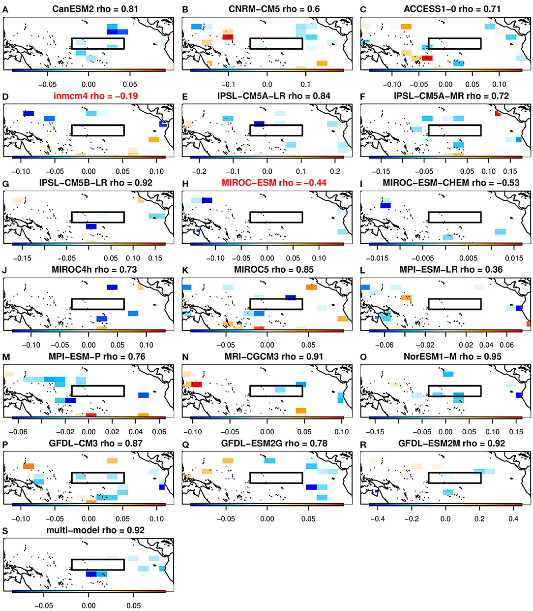
Figure 5. The β coefficients selected by lasso for predicting week 3–4 ENSO-forced temperature pattern using grid points in the Tropical Pacific. The black boxes indicates the Nino3.4 index. Red model names indicate the models that individually had a minimum NMSE greater than 1. (A) CanESM2 rho= 0.81. (B) CNRM-CM5 rho = 0.6. (C) ACCESS1-0 rho = 0.71. (D) inmcm4 rho = −0.19. (E) IPSL-CM5A-LR rho = 0.84. (F) IPSL-CM5A-MR rho = 0.72. (G) IPSL-CM5B-LR rho =0.92. (H) MIROC-ESM rho = −0.44. (I) MIROC-ESM-CHEM rho = −0.53. (J) MIROC4h rho = 0.73. (K) MIROC5 rho = 0.85. (L) MPI-ESM-LR rho = 0.36. (M) MPI-ESM-P rho = 0.76. (N) MRI-CGCM3 rho = 0.91. (O) NorESM1-M rho = 0.95. (P) GFDL-CM3 rho = 0.87. (Q) GFDL-ESM2G rho = 0.78. (R) GFDL-ESM2M rho = 0.92. (S) Multi-model rho = 0.92.

FIGURE 6

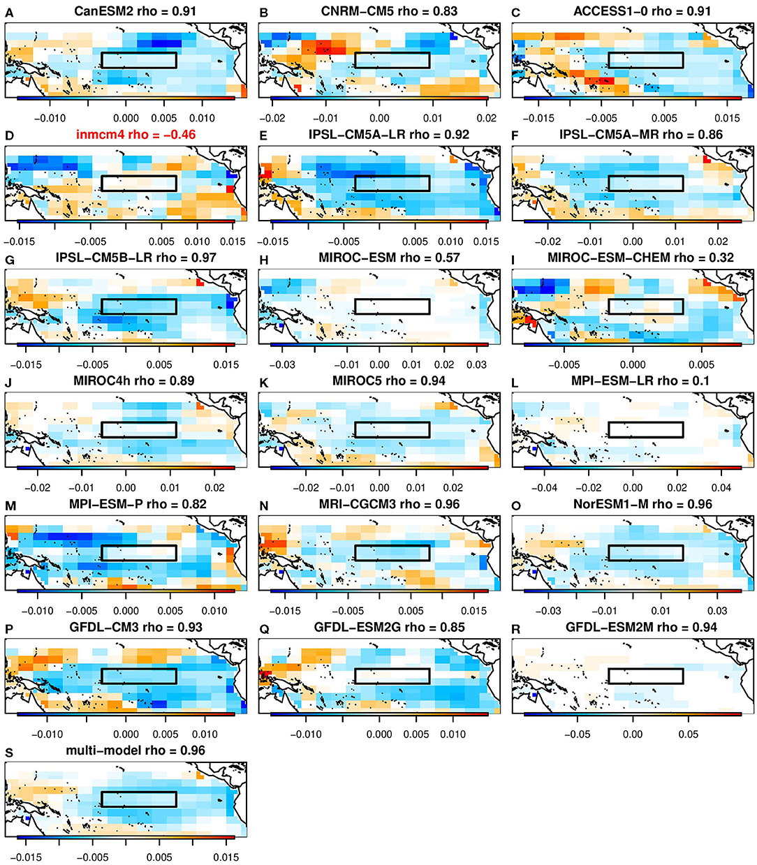
Figure 6. The β coefficients selected by ridge regression for predicting week 3–4 ENSO-forced temperature pattern using grid points in the Tropical Pacific. The black boxes indicates the Nino3.4 index. Red model names indicate the models that individually had a minimum NMSE greater than 1. (A) CanESM2 rho= 0.91. (B) CNRM-CM5 rho = 0.83. (C) ACCESS1-0 rho = 0.91. (D) inmcm4 rho = −0.46. (E) IPSL-CM5A-LR rho = 0.92. (F) IPSL-CM5A-MR rho = 0.86. (G) IPSL-CM5B-LR rho =0.97. (H) MIROC-ESM rho = 0.57. (I) MIROC-ESM-CHEM rho = 0.32. (J) MIROC4h rho = 0.89. (K) MIROC5 rho = 0.94. (L) MPI-ESM-LR rho = 0.1. (M) MPI-ESM-P rho = 0.82. (N) MRI-CGCM3 rho = 0.96. (O) NorESM1-M rho = 0.96. (P) GFDL-CM3 rho = 0.93. (Q) GFDL-ESM2G rho = 0.85. (R) GFDL-ESM2M rho = 0.94. (S) Multi-model rho = 0.96.

In these figures, there are models that are unable to produce a statistical model with a NMSE less than 1 for any λ—that is, using lasso or ridge regression they are unable to make a better week 3–4 prediction in observations compared to observed climatology. Those models also have a negative correlation with the Nino3.4 index. Using lasso, this applies to the inmcm4 and MIROC-ESM models (Figures 5 D,H). Using ridge regression, this applies to the inmcm4 model (Figure 6D).

The analysis presented here could, with further refinement, be used as a new kind of diagnostic for model output. For instance, we found that machine learning models trained on inmcm4 and MIROC-ESM had no skill in predicting the ENSO-forced pattern for any choice of λ, in contrast to other CMIP5 models. In the model description of its climatology for each of the two models [see Volodin et al. (2010) for the inmcm4 model and Watanabe et al. (2011) for the MIROC-ESM model], the authors point out that their simulated annual SSTs are similar to other climate models. Additionally, a statistical analysis of the variance and correlation of individual CMIP5 models' El Niño teleconnections done by Weare (2013) indicates that these models performed comparably to other CMIP5 models. Ordinarily, the lack of sub-seasonal forecasts from dynamical models would make validation impossible, but here we use model output as training data for subseasonal predictions, which yields a kind of proxy for subseasonal forecasts that can be validated against observations without explicitly creating initialized subseasonal forecasts from these dynamical models.

4.2. Tropical Pacific, EOF Predictors

Since the above forecasts are only modestly better than the Nino3.4 index, we explore alternative predictors, particularly EOFs. The first EOF has a correlation of 0.98 with the Nino3.4 index, so in theory the regression model should be able to use the other EOFs to make a better prediction than the Nino3.4 index alone.

Using the Tropical Pacific EOFs to make a prediction, lasso's prediction is just the first EOF. It has a NMSE of 0.894 and its random walk test is not shown but is like Figure 3C (indistinguishable from a prediction made with the Nino3.4 index). Ridge regression does select a larger amplitude for the first EOF but includes all of the rest as well. The result of this is a low correlation with the Nino3.4 index (ρ = 0.53), a NMSE of 0.936 (worse than the Nino3.4 index's NMSE) and a random walk test like Figure 3D (a worse prediction than the Nino3.4 index for the entire month of December).

Although ridge regression's β spatial pattern (Figure 4C) looks nothing like the Nino3.4 index and its correlation confirms the dissimilarity, we cannot conclude just by visual inspection that this will be a poor predictor. To illustrate the problem with visual inspection of beta coefficients, we artifically construct a pattern made up of two EOFs, the first EOF with an amplitude of −1 and the 100th EOF with an amplitude of 0.3. The result, shown in Figure 7, reveals a β spatial pattern that has a correlation of 0.95 with the Nino3.4 index, despite looking completely random. This example exploits the fact that the variance of the leading and trailing EOFs differ by several orders of magnitude, so a relatively large β can be attached to the trailing EOF but still produce a prediction dominated by the leading EOF.

FIGURE 7

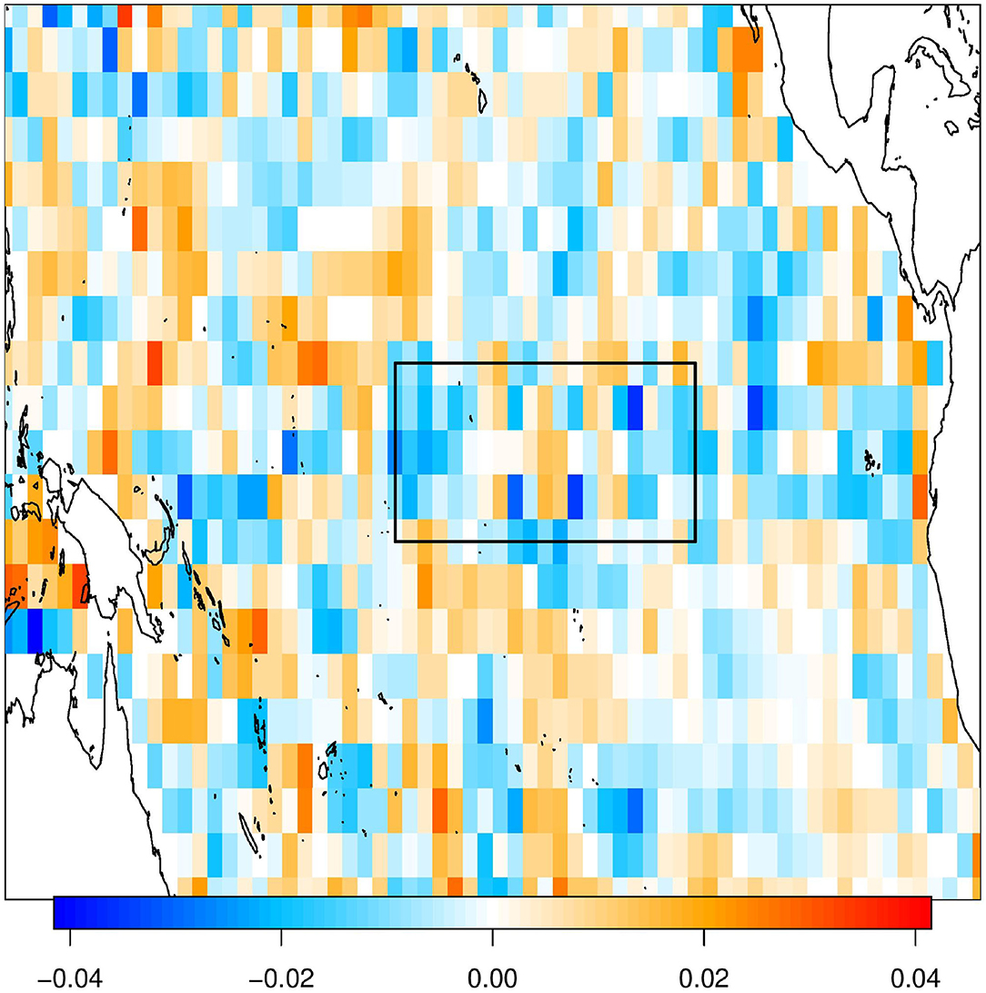
Figure 7. A contrived example of β coefficients that yield predictions with a high correlation with the Nino3.4 index (0.95) while bearing little similarity to the leading EOF of SST.

4.3. Atlantic Plus Pacific, EOF Predictors

It is possible that expanding the domain to include the Pacific extratropics and the Atlantic could improve our prediction skill. Using EOFs in this domain, the first EOF has a correlation of 0.97 with the Nino3.4 index, so like the previous section, by giving lasso and ridge additional predictors they might be able to make a better prediction than the Nino3.4 index alone.

With the domain expanded to the Atlantic plus Pacific, predictions are somewhat improved compared to the tropical Pacific alone. Ridge regression especially sees an improvement with a NMSE of 0.879 and a random walk test that is like Figure 3C (indistinguishable from the Nino3.4 index). Curiously, its correlation with the Nino3.4 index is relatively low (only 0.78) although its NMSE is similar to that of the Nino3.4 index. Despite its moderate correlation with the Nino3.4 index, ridge regression's β associated with the first EOF has a very small amplitude.

Lasso puts a large emphasis on the first EOF, although 7 other EOFs are included in the prediction. Lasso's prediction has a NMSE of 0.886 and a correlation of 0.94 with the Nino3.4 index. It's random walk test is also like Figure 3C.

4.4. Both Domains, Laplacian Predictors

Physically, teleconnections are set up by large scale structures. We can define Laplacian eigenvectors for the tropical Pacific domain as well as for the Atlantic plus Pacific domains. The first few Laplacians for each domain is shown in Figure 8. Truncating at 100 Laplacians gives us sufficient resolution without being computationally overwhelming. The SST represented by 100 Laplacians is

$\begin{array}{ll}S=X{E}^T& (7)\end{array}$

where S (time × space) is the time series of the SST field represented by a linear combination of 100 Laplacians, X (time × 100) is the time series of the 100 SST Laplacians, and E (space × 100) is the spatial patterns of the 100 Laplacians.

FIGURE 8

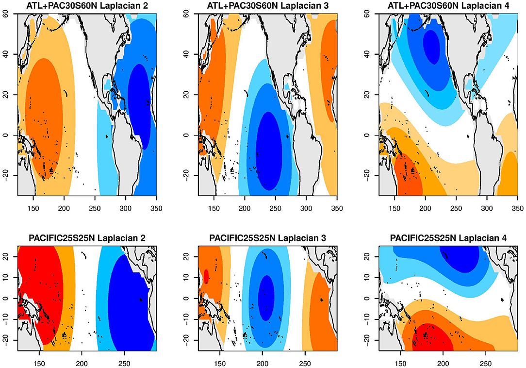
Figure 8. Laplacian eigenvectors 2–4 for the Atlantic plus Pacific (top), and for the tropical Pacific (bottom) domains. The first pattern for each basin is the spatial average over the domain and is not shown.

When applying the Laplacians as a basis set over the Atlantic plus Pacific, both algorithms' predictions get much worse. Lasso has a NMSE of 0.918 and ridge regression has a NMSE of 0.914. Both of their random walk tests are like Figure 3D (worse than the Nino3.4 index). What makes this case notable is that both predictions have a large correlation with the Nino3.4 index (0.92 for ridge and 0.93 for lasso) but are dramatically outperformed by the Nino3.4 index.

When making a prediction from the Tropical Pacific using SST Laplacians as the predictors, lasso gives a NMSE of 0.864 and ridge regression gives a NMSE of 0.871. The results of the random walk test are very similar for both lasso and ridge regression and is shown in Figure 3A (better than the Nino3.4 index in late January and possibly also in mid-December).

4.5. Weighted Tropical Pacific, Laplacians Predictors

When using Laplacians in the Tropical Pacific, the structure of the βs selected is dominated by small-scale noise, which is not physically realistic. It is possible to modify LASSO so that large-scale structures are preferentially selected. There are any number of ways to do this. It turns out that the variance of the Laplacian time series drops almost monotonically as the spatial scale of the Laplacian decreases (i.e., the Laplacian number increases). Knowing this, we chose to weight the choice of β by the inverse of the variance, so that the βs associated with the large-scale Laplacians (which have more variance) would have a larger amplitude. The resulting β patterns (Figures 4K,L) are larger scale and therefore we would consider them more physically realistic. These larger scale structures seem like they would be able to better represent the Nino3.4 signal than the smaller scale structures we get when we don't weight the predictors, but the correlation with the Nino3.4 index is almost the same as without the weighting.

Both the lasso and the ridge regression predictions have a NMSE of 0.870, which are also almost the same as without the weighting. The random walk tests are similar for both and are represented by Figure 3C (indistinguishable from the Nino3.4 index). Besides the more physically realistic β patterns, we found no advantage to using this alternative weighting scheme for selecting the beta coefficients.

5. Conclusions

This paper shows that skillful predictions of the “ENSO-forced” pattern of week 3–4 2 m temperatures over CONUS can be made based on the Nino3.4 index alone. To identify better prediction models, various machine learning models using sea surface temperatures as predictors were developed. In addition, machine learning models were trained on observations and on long control simulations. We find the machine learning models trained on climate model simulations are more skillful than machine learning models trained on observations. Presumably, the reason for this is that the training sample from climate model simulations is orders of magnitude larger than training sample available from observations. Initialized predictions from a dynamical model, namely the CFSv2 model, also were examined. With amplitude correction, the skill of CFSv2 hindcasts of this pattern were comparable to the skill of predictions from Nino3.4 and machine learning models.

The skills of machine learning models and a simple prediction based on the Nino3.4 index are very close to each other. To ascertain if one is better than the other, we performed a careful statistical assessment of whether the machine learning predictions were better than predictions based on the Nino3.4 index alone. To avoid serial correlation, the test was performed for each initial start date separately. We found that the best machine learning predictions were significantly more skillful for only about 10% of the cases, while for most other start dates the hypothesis of equally skillful predictions could not be rejected. Our general conclusion is that although the best predictions of the ENSO-forced pattern come from machine learning models trained on long climate simulations, the skill is only “modestly” better than predictions based on the Nino3.4 index alone.

Various attempts were made to interpret the source of predictability in the machine learning predictions. Lasso is usually promoted as being better for interpretation due to its ability to set the amplitude of some predictors to zero. However, when the predictors are correlated grid points, lasso selects isolated grid points whereas ridge regression yields smooth, large-scale patterns, making the latter more physically realistic. When selecting uncorrelated predictors such as EOFs, lasso retains its interpretability advantage. Nevertheless, interpretation of the regression weights can be very misleading. Specifically, very different maps of β-coefficients can produce virtually the same prediction. To illustrate this, we generated an artificial set of beta coefficients in Figure 7 that yields a high correlation with the Nino3.4 index (ρ = 0.95) but whose appearance is very different from the canonical ENSO pattern. Another factor is that if the predictors are correlated, then the predictors selected by lasso can be very sensitive to the training sample. Despite this, it is worth noting that in contrast to the β-coefficients, the regression patterns between the machine learning predictions and model SSTs are very robust and all emphasize the tropical Pacific ENSO pattern (Figure 9).

FIGURE 9

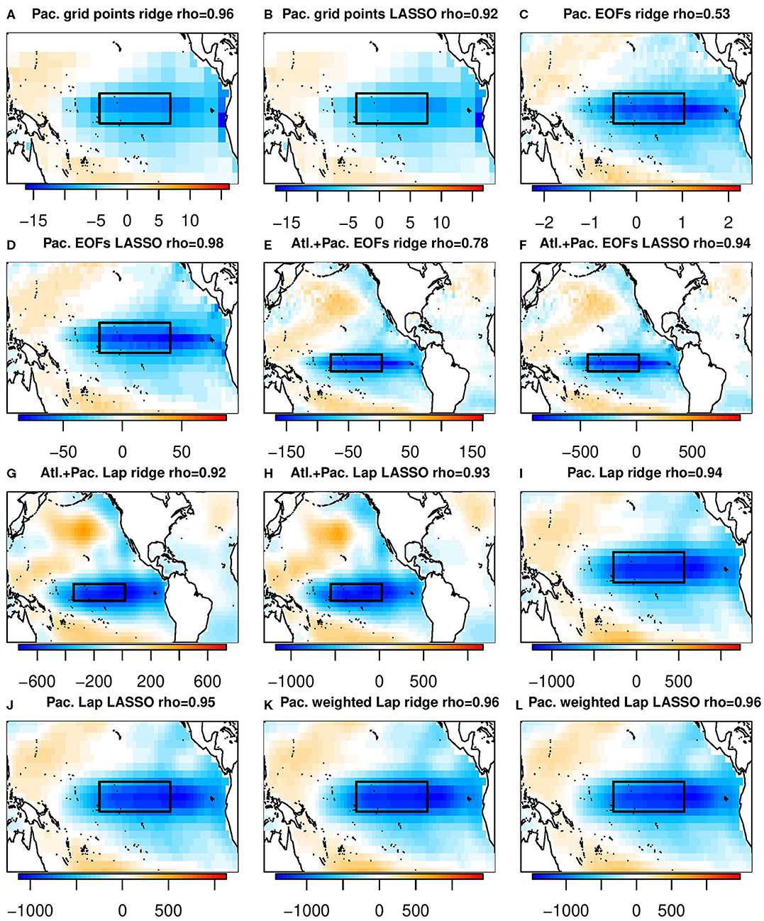
Figure 9. The regression coefficient between each machine learning prediction and the local SST, calculated by regressing the prediction against observed SST. As in Figure 4, titles of the individual panels indicate the domain, basis set, machine learning algorithm used, and the correlation between the resulting prediction and the Nino3.4 index. (A) Pac. grid points ridge rho = 0.96. (B) Pac. grid points LASSO rho = 0.92. (C) Pac. EOFs ridge rho = 0.53. (D) Pac. EOFs LASSO rho = 0.98. (E) Alt+Pac. EOFs ridge rho = 0.78. (F) Alt+Pac. EOFs LASSO rho = 0.94. (G) Alt+Pac. Lap ridge rho = 0.92. (H) Alt+Pac. Lap LASSO rho = 0.93. (I) Pac. Lap ridge rho = 0.94. (J) Pac. Lap LASSO rho = 0.95. (K) Pac. weighted Lap ridge rho = 0.96. (L) Pac. weighted Lap LASSO rho = 0.96.

This machine learning framework is extremely versatile—there is no essential reason why it could not be used to predict other variables, use other variables as predictors, or make predictions at different time scales. As an example, a subseasonal prediction of temperature could be attempted using snow cover anomalies as well as SST anomalies in the winter. A major caveat to this framework as a whole is that dynamical models are not perfect—if there is no signal for the machine learning to train upon then it will never be able to predict observations using that predictor. This could also be a new way to validate dynamical models—some models used in this study were not skillful at making subseasonal predictions of observations.

Data Availability Statement

The original contributions presented in the study are included in the article/supplementary material, further inquiries can be directed to the corresponding author/s.

Author Contributions

PB performed the computations. PB and TD contributed equally to the writing of this manuscript. Both authors provided critical feedback and helped shape the research, analysis, and manuscript.

Funding

This research was supported primarily by the National Science Foundation (AGS-1822221). Additional support was provided from National Science Foundation (AGS-1338427), National Aeronautics and Space Administration (NNX14AM19G), the National Oceanic and Atmospheric Administration (NA14OAR4310160). The views expressed herein do not necessarily reflect the views of these agencies.

Conflict of Interest

The authors declare that the research was conducted in the absence of any commercial or financial relationships that could be construed as a potential conflict of interest.

Publisher's Note

All claims expressed in this article are solely those of the authors and do not necessarily represent those of their affiliated organizations, or those of the publisher, the editors and the reviewers. Any product that may be evaluated in this article, or claim that may be made by its manufacturer, is not guaranteed or endorsed by the publisher.

Acknowledgments

We acknowledge the World Climate Research Programme's Working Group on Coupled Modeling, which is responsible for CMIP, and we thank the climate modeling groups (listed in Table 1 of this paper) for producing and making available their model output. For CMIP the U.S. Department of Energy's Program for Climate Model Diagnosis and Intercomparison provides coordinating support and led development of software infrastructure in partnership with the Global Organization for Earth System Science Portals.

We acknowledge the agencies that support the SubX system, and we thank the climate modeling groups (Environment Canada, NASA, NOAA/NCEP, NRL, and University of Miami) for producing and making available their model output. NOAA/MAPP, ONR, NASA, NOAA/NWS jointly provided coordinating support and led development of the SubX system.

We would like to acknowledge Sebastian Sippel for his insights into the interpretability of ridge regression vs. lasso. We would like to acknowledge Michael Tippett for his helpful comments throughout the course of this research. We would like to thank two reviewers whose comments significantly improved this manuscript.

References

Baldwin, M. P., Ayarzagüena, B., Birner, T., Butchart, N., Butler, A. H., Charlton-Perez, A. J., et al. (2021). Sudden stratospheric warmings. Rev. Geophys. 59:e2020RG000708. doi: 10.1029/2020RG000708

CrossRef Full Text | Google Scholar

Barnston, A. G., Chelliah, M., and Goldenberg, S. B. (1997). Documentation of a highly enso-related SST region in the equatorial pacific: research note. Atmos. Ocean 35, 367–383. doi: 10.1080/07055900.1997.9649597

CrossRef Full Text | Google Scholar

Copas, J. B. (1983). Regression, prediction and shrinkage. J. R. Stat. Soc. Ser. B 45, 311–354. doi: 10.1111/j.2517-6161.1983.tb01258.x

CrossRef Full Text | Google Scholar

DelSole, T., and Tippett, M. K. (2014). Comparing forecast skill. Mnthly Weather Rev. 142, 4658–4678. doi: 10.1175/MWR-D-14-00045.1

CrossRef Full Text | Google Scholar

DelSole, T., and Tippett, M. K. (2015). Laplacian eigenfunctions for climate analysis. J. Clim. 28, 7420–7436. doi: 10.1175/JCLI-D-15-0049.1

CrossRef Full Text | Google Scholar

DelSole, T., and Tippett, M. K. (2016). Forecast comparison based on random walks. Mnthly Weather Rev. 144, 615–626. doi: 10.1175/MWR-D-15-0218.1

CrossRef Full Text | Google Scholar

DelSole, T., Trenary, L., Tippett, M. K., and Pegion, K. (2017). Predictability of week-3-4 average temperature and precipitation over the contiguous United States. J. Clim. 30, 3499–3512. doi: 10.1175/JCLI-D-16-0567.1

CrossRef Full Text | Google Scholar

DelSole, T., Yan, X., Dirmeyer, P. A., Fennessy, M., and Altshuler, E. (2014). Changes in seasonal predictability due to global warming. J. Clim. 27, 300–311. doi: 10.1175/JCLI-D-13-00026.1

CrossRef Full Text | Google Scholar

Geisler, J. E., Blackmon, M. L., Bates, G. T., and Muñoz, S. (1985). Sensitivity of january climate response to the magnitude and position of equatorial pacific sea surface temperature anomalies. J. Atmos. Sci. 42, 1037–1049. doi: 10.1175/1520-0469(1985)042<1037:SOJCRT>2.0.CO;2

CrossRef Full Text | Google Scholar

Guo, Z., Dirmeyer, P. A., and DelSole, T. (2011). Land surface impacts on subseasonal and seasonal predictability. Geophys. Res. Lett. 38:L24812. doi: 10.1029/2011GL049945

CrossRef Full Text | Google Scholar

Hastie, T., Tibshirani, R., and Friedman, J. H. (2009). The Elements of Statistical Learning: Data Mining, Inference, and Prediction, 2nd Edn. New York, NY: Springer. doi: 10.1007/978-0-387-84858-7

CrossRef Full Text | Google Scholar

Higgins, R. W., Kim, H.-K., and Unger, D. (2004). Long-lead seasonal temperature and precipitation prediction using tropical pacific sst consolidation forecasts. J. Climate 17, 3398–3414. doi: 10.1175/1520-0442(2004)017<3398:LSTAPP>2.0.CO;2

CrossRef Full Text | Google Scholar

Hwang, J., Orenstein, P., Cohen, J., Pfeiffer, K., and Mackey, L. (2019). Improving subseasonal forecasting in the western U.S. with machine learning, in Proceedings of the 25th ACM SIGKDD International Conference on Knowledge Discovery &Data Mining, KDD '19 (New York, NY: Association for Computing Machinery), 2325–2335. doi: 10.1145/3292500.3330674

CrossRef Full Text | Google Scholar

Jin, F., and Hoskins, B. J. (1995). The direct response to tropical heating in a baroclinic atmosphere. J. Atmos. Sci. 52, 307–319. doi: 10.1175/1520-0469(1995)052<0307:TDRTTH>2.0.CO;2

CrossRef Full Text | Google Scholar

Johnson, N. C., Collins, D. C., Feldstein, S. B., L'Heureux, M. L., and Riddle, E. E. (2014). Skillful wintertime north American temperature forecasts out to 4 weeks based on the state of ENSO and the MJO. Weather Forecast. 29, 23–38. doi: 10.1175/WAF-D-13-00102.1

CrossRef Full Text | Google Scholar

McPhaden, M. J., Busalacchi, A. J., and Anderson, D. L. (2010). A toga retrospective. Oceanography 23, 86–103. doi: 10.5670/oceanog.2010.26

CrossRef Full Text | Google Scholar

National Research Council (2010). Assessment of Intraseasonal to Interannual Climate Prediction and Predictability. The National Academies Press, Washington, DC.

Google Scholar

Pegion, K., Kirtman, B. P., Becker, E., Collins, D. C., LaJoie, E., Burgman, R., et al. (2019). The subseasonal experiment (subx): a multimodel subseasonal prediction experiment. Bull. Am. Meteorol. Soc. 100, 2043–2060. doi: 10.1175/BAMS-D-18-0270.1

CrossRef Full Text | Google Scholar

Shukla, J., and Kinter, J. L. (2006). Predictability of seasonal climate variations: a pedagogical review, in Predictability of Weather and Climate, eds T. Palmer and R. Hagedorn (Cambridge: Cambridge University Press), 306–341. doi: 10.1017/CBO9780511617652.013

CrossRef Full Text | Google Scholar

Slater, L. J., Villarini, G., and Bradley, A. A. (2019). Evaluation of the skill of north-American multi-model ensemble (NMME) global climate models in predicting average and extreme precipitation and temperature over the continental USA. Clim. Dyn. 53, 7381–7396. doi: 10.1007/s00382-016-3286-1

CrossRef Full Text | Google Scholar

Sobolowski, S., Gong, G., and Ting, M. (2007). Northern hemisphere winter climate variability: response to north American snow cover anomalies and orography. Geophys. Res. Lett. 34:L16825. doi: 10.1029/2007GL030573

CrossRef Full Text | Google Scholar

Tibshirani, R. (1996). Regression shrinkage and selection via the lasso. J. R. Stat. Soc. Ser. B 58, 267–288. doi: 10.1111/j.2517-6161.1996.tb02080.x

CrossRef Full Text | Google Scholar

Volodin, E. M., Dianskii, N. A., and Gusev, A. V. (2010). Simulating present-day climate with the INMCM4.0 coupled model of the atmospheric and oceanic general circulations. Izvestiya Atmos. Ocean. Phys. 46, 414–431. doi: 10.1134/S000143381004002X

CrossRef Full Text | Google Scholar

Watanabe, S., Hajima, T., Sudo, K., Nagashima, T., Takemura, T., Okajima, H., et al. (2011). MIROC-ESM 2010: model description and basic results of cmip5-20c3m experiments. Geosci. Model Dev. 4, 845–872. doi: 10.5194/gmd-4-845-2011

CrossRef Full Text | Google Scholar

Weare, B. C. (2013). El niño teleconnections in CMIP5 models. Clim. Dyn. 41, 2165–2177. doi: 10.1007/s00382-012-1537-3

CrossRef Full Text | Google Scholar