Emerging Skill in Multi-Year Prediction of the Indian Ocean Dipole

Introduction

The Indian Ocean Dipole (IOD) is an inter-annual coupled ocean–atmosphere phenomenon in the tropical Indian Ocean that peaks during the boreal fall season (September to November; SON). Positive IODs are associated with anomalously warmer western Indian Ocean and anomalously cooler eastern Indian Ocean. Negative IOD events are associated with opposite anomalous sea surface temperatures (SSTs) across the Indian Ocean (Saji et al., 1999; Webster et al., 1999; Murtugudde et al., 2000). The IOD is a well-known driver of global climate (Saji and Yamagata, 2003). In addition to affecting the neighboring Maritime Continent to the east and East Africa to the west (Behera et al., 2005), the positive IOD events, for example, have been associated with reduced rainfall over western and southern Australia (Ashok et al., 2003; Ashok and Saji, 2007; Cai et al., 2011), enhanced seasonal Indian summer monsoon (ISM) rainfall (Ashok et al., 2001; Ashok and Saji, 2007), and climates of even distant regions of South America (Chan et al., 2008) and Europe (Hardiman et al., 2020). In addition to its own coupled dynamics (Gualdi et al., 2003; Yamagata et al., 2004; Behera et al., 2006; Ha et al., 2017; Tanizaki et al., 2017; Saji, 2018; Marathe et al., 2021), the IOD is suggested to be triggered by other inter-annual processes such as the El Niño–Southern Oscillation (ENSO), the dominant climate driver from the tropics.

Attempts to predict the IOD on a seasonal scale have been on-going for about two decades (Iizuka et al., 2000; Shinoda et al., 2004; Luo et al., 2007; Doi et al., 2016) and have met with relatively shorter lead time skills, the highest being of 4 months. This is in contrast to the 12–17 months of lead prediction skill for the ENSO as shown in recent studies (Barnston et al., 2012; Park et al., 2018; Tang et al., 2018). Several papers claim that prediction skills for the IOD and ENSO are linked and intertwined (Wajsowicz, 2005; Izumo et al., 2010; Luo et al., 2010).

The emerging discipline of decadal prediction, i.e., prediction of climate information for the near future, shows great promise for societal needs and economic policymakers. Decadal prediction lies between weather prediction and climate projection. Therefore, decadal prediction has to resolve initial value problems like in weather prediction and seasonal to inter-annual forecasts and climate variability and trends effective from boundary conditions, including slow varying oceanic processes, snow cover, and anticipated changes in anthropogenic greenhouse gases and aerosols (Meehl et al., 2009, 2014; Smith et al., 2013; Boer et al., 2016). Interestingly, the inter-annual ENSO and the IOD can also be modulated by decadal processes (Ashok et al., 2004; Tozuka et al., 2007). Such processes should enhance the decadal prediction skill of these inter-annual events.

Given the limited lead skill of the IOD on seasonal scales, its prediction at multi-year lead times is exceptionally challenging. Remarkably, in this study, we show that two model hindcasts from the CMIP5 (Coupled Model Intercomparison Project—Phase 5) decadal prediction datasets are found to show successful prediction skill for IOD events. These sets give us an opportunity to track the lead prediction skill of an event at a lead of up to 2 years.

Data and Methods

Data

We have mainly used a sub-set of the decadal hindcast outputs from the CMIP5 decadal runs (Meehl et al., 2009, 2014; Taylor et al., 2012; Smith et al., 2013; Boer et al., 2016). These runs have anthropogenic and natural forcing in them, and comprise several independent decade-long ensemble-runs by each model. For example, the four members of the first ensemble are initialized in 1960 and run up to 1970 (Figure 1). Such runs are available with initial conditions from 1960 to 2011. Together, we have 51 ensemble members of decadal hindcasts for each model, each differing from the other in the initialization year (from 1960 to 2011). For each model, we average multiple ensembles with same initialization dates. These averages are referred to as the model hindcasts for the initial conditions of that particular year. The models, whose hindcasts we consider, are the CanCM4 (Merryfield et al., 2013), MIROC5 (Watanabe et al., 2010), BCC-CSM (Wu et al., 2013), and the GFDL (Delworth et al., 2006; Zhang et al., 2007) models. The output data from all the models are divided into 10 groups depending on the year after initialization (Figure 1). Yr1, yr2, yr3… indicate 1, 2, 3 … year(s) after initialization.

FIGURE 1

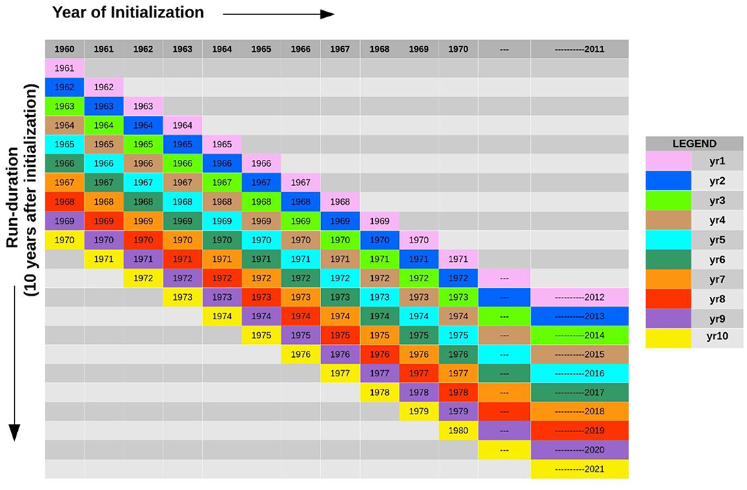
Figure 1. The output data from all the models are divided into 10 groups depending on the year after initialization. Yr1, yr2, yr3… indicates 1, 2, 3 … year(s) after initialization, which is represented by individual colors.

We used Hadley Center Sea Ice and Sea Surface Temperature (HadISST; Rayner et al., 2003) and Ocean Reanalysis data from the European Center for Medium-Range Weather Forecasts (ORAS4; Balmaseda et al., 2013) for ocean temperatures. As for ENSO indices, we calculate the NINO3 and NINO4 indices as anomalies of SSTs in area averaged over the boxes 150–90°W, 5°S−5°N and 160°E−150°W, 5°S−5°N, respectively. We calculate the Indian Ocean Dipole Mode Index (IODMI) as the SST gradient between the western equatorial Indian Ocean (50–70°E and 10°S−10°N) and the south-eastern equatorial Indian Ocean (90–110°E and 10°S−0°). We take into consideration the IODMI only during the months of September to November as the IOD peaks during this season.

Statistical Methods

We have carried out correlation and regression analysis. We have used the two-tailed Student's t-test to determine the significance of the correlation coefficients. We ascertained the robustness of the skills by applying a boot-strapping test for 1,000 simulations (using NCL) and found our results to be significant at 90% for up to 4 years. For verifying the skill of persistence for both the models and observations, we use the auto-correlation (Supplementary Figure 1). To illustrate briefly, say in the case of CanCM4, we correlate the predicted IODMI at lead 1 with that at lead 2 to get the persistence skill at lead 1. Similarly, the persistence skill at lead 2 is obtained by correlating the predicted IODMI at lead 0 with that at lead 2, and so on. We have used the Empirical Orthogonal Function (EOF) analysis technique (von Storch and Zwiers, 1999) to determine the dominant patterns of spatio-temporal variability in the equatorial Indian Ocean, as an additional analysis to compare the simulated IODs with the observations. The EOF analysis is a multivariate statistical technique to calculate the eigenvalues and eigenvectors of a spatially weighted anomaly covariance matrix. The corresponding eigenvalues quantify the variance percent explained by each pattern, which is, by definition, orthogonal to the other patterns.

To have an estimate of the inter-annual variability of IOD that could be attributed to the Southern Ocean (20°W:50°E; 60°S:40°S), we projected the IODMI on to the corresponding area-averaged subsurface temperatures (vertically averaged over 300–800 m depth), i.e., through a regression analysis, and measured the goodness-of-fit (figure not shown).

Results

Lead Prediction Skills for ENSO and IOD

ENSO events peak during the boreal winter (through December), while the IOD events peak during boreal fall (September–November). Our analysis shows that the hindcasts analyzed in this study (Figure 2A) predict the peak NINO3 index (Trenberth, 1997) significantly at leads up to 12–13 months, in agreement with earlier studies (Sun et al., 2018; Pal et al., 2020).

FIGURE 2

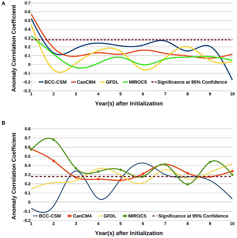
Figure 2. (A) Anomaly correlations between observed NINO3 index with the corresponding predicted NINO3 index at different lead years for various models, shown in different colors. The significant correlation value at 95% confidence level is 0.27 and is shown by dashed lines. Details of how the correlations at different leads were obtained, from the sets of ~51 year-long decadal prediction runs with different initial years, are available from section Statistical Methods and Figure 1. (B) Same as (A) but for the IODMI. The lines with circles in (B) are the two models of interest for this study.

Surprisingly, the hindcasts from the MIROC5 and CanCM4 predict the IODMI during the fall season with significant lead prediction skill for at least 2–3 years (Figure 2B). The skill levels for most of the lead times are not only statistically significant at the 95% confidence level from a two-tailed Student's t-test but also are better than persistence (Supplementary Figure 1). While the lead prediction skills of the IODMI from the CanCM4 fall below 95% confidence level at 4–5-year leads, these skill levels are still significant at a 90% confidence level. The MIROC5 also shows a weak skill for the eighth year, still significant at 80% confidence level.

It is noteworthy that this skill is present despite the maximum lead predictability of only 1 year for the NINO3 index in all the models. We also ascertain that the maximum lead time skill for the NINO4 is similar to those for the NINO3 index. The ISM rainfall is an ocean–atmosphere coupled phenomenon occurring every year from June to September bringing copious amount of rainfall over the Indian subcontinent. ISM is strongly influenced by ENSO and IOD, along with other factors. Our study shows that ISM has no predictability in the analyzed models, presumably due to model inadequacies in representing monsoon processes (figure not shown). Nevertheless, rainfall predictions could be improved by exploiting known statistical relationships between ENSO-ISM or IOD-ISM (Jourdain et al., 2013; Swapna et al., 2015; Dutta and Maity, 2018).

Fidelity of the Simulated IOD

To further ascertain whether the IODMI computed from the two hindcast datasets represents some of the observed features of the IOD (Yamagata et al., 2003), we compare the second leading simulated EOF modes of the SST from the hindcasts of MIROC5 and CanCM4 with that from the corresponding observations. Figure 3, derived from the EOF analysis at 1-year lead, shows that the models indeed capture the observed dominant IOD variance pattern associated with the EOF2 in terms of the location of the two centers of action. The simulated variance explained by this statistical mode from the MIROC5 is 12.2%, comparable with the corresponding observed value of 12% (Saji et al., 1999; Ashok et al., 2004). EOF2 of CanCM4 is 27.4%, which is higher than the expected value as the dipole-like structure shows more spread in the eastern Indian Ocean (Figure 3). The simulated EOF1, associated with Indian Ocean Basin mode, and the corresponding variance explained are also realistic.

FIGURE 3

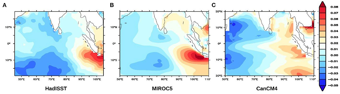
Figure 3. The second mode from the EOF analysis of the tropical Indian Ocean SST, from (A) HadISST (1961–2011 period). (B,C) are the same as that of (A) but derived from MIROC5 and CanCM4 hindcasts for the same period (also see Supplementary Figure 2).

Source of the IOD Prediction Skill

A question arises as to what processes are responsible for the IOD predictability. Earlier studies have shown that the key component of improved decadal prediction lies in ocean physical processes, which internally generate decadal climate variability (Meehl et al., 2014; Farneti, 2017). Thus, the memory of the upper ocean (~800 m) provides an improved predictability of SST variability in models on decadal timescales (Yeager et al., 2012; Wang et al., 2014). Motivated by these, we looked for a source of predictability of IOD at several levels in the subsurface temperature (every 50 m). We found the maximum signal in the Southern Ocean at 300 to 800 m depth 7–10 years before the occurrence of the IOD event. From an analysis of the ORAS4 and SODA3 reanalysis datasets, we find a signal for the IODMI in the Southern Ocean. This is evidenced by significant correlations between depth-averaged 300–800 m temperatures in the Southern Ocean, which lead the IODMI by 10–6 years, respectively (Figure 4). The significant positive correlations in the Southern Ocean indicate that a positive temperature anomaly in the Southern Ocean leads to a positive IOD event after 8–10 years, whereas a similar lead negative correlation coefficient in the Southern Ocean indicates a negative IOD event after such a time period. The signal leading the IODMI first appears in the sub-surface temperatures of the Southern Ocean just south-west of Africa between the depths of 300–800 m, 10 years before the occurrence of the IOD event. This signal is seen to propagate toward the east along the Antarctic Circumpolar Current (ACC, or West wind drift) to about 50–60°E about 6 years prior to the IOD event. From here, the signal in the heat content further propagates north, along the east of Madagascar, all the way to the Somali coast in a pathway that is coincident with the East Madagascar undercurrent (EMUC)—an intermediate undercurrent at the depth of thermocline and below. The period of the propagation is in agreement with the EMUC as described by Nauw et al. (2008). The EMUC transports about 2.8 ± 1.4 Sv of intermediate water equatorward. The signal upwells to the surface near Somalia (Somali upwelling) along with its propagation north (Figure 5).

FIGURE 4

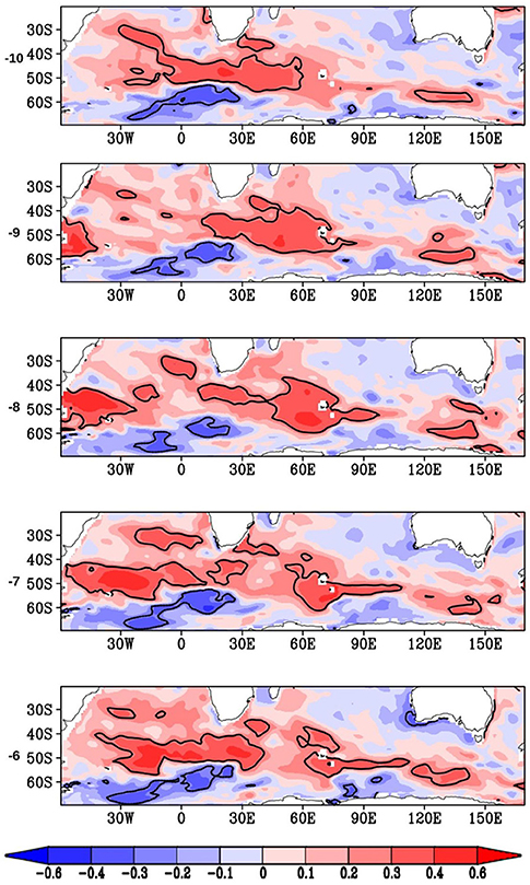
Figure 4. Spatial distribution of the anomaly correlation of HadISST derived IODMI with vertically averaged subsurface temperatures from ORAS4 (over 300–800 m depth) from previous years averaged annually. The “lag number” is the years over which the IOD lags the Southern Ocean signal. In all panels, significant correlations at 95% confidence are shown as contour lines (value at 0.27).

FIGURE 5

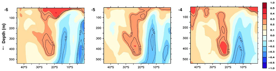
Figure 5. Vertical distribution of anomaly correlation of IODMI with previous years' subsurface temperatures, averaged annually over longitudes 50–100°E. Significant correlations at 90% confidence (0.23) and at 95% confidence (0.27) are contoured.

The propagation of the signal from the deeper layers in the extra-tropics to the surface layers in the equatorial region can be explained by the Indian Ocean Meridional Overturning Circulation (IOMOC; Wang et al., 2014). The time period of the propagation is in agreement with the IOMOC. From the Somali coast, the lead heat content signal is seen to move east, reaching the central equatorial Indian Ocean 3 years before the IOD event. The signal remains in the equatorial Indian Ocean for the last 2–3 years before the occurrence of the IOD event (Figure 6). Furthermore, our correlation in Figure 6 suggests an anomalous SST structure of opposite polarity in the equatorial Indian Ocean about a year before the occurrence of an IOD event. This is in conformation with Saji et al. (1999), who not only note a tight coupling between the intensity of the SST dipole anomaly and zonal wind anomaly but emphasize on a biennial tendency. The biennial tendency of the IOD is also noted by Meehl and Arblaster (2001), Ashok et al. (2003), etc. It is intriguing why the signal from the sub-surface at the equator does not manifest as an IOD event immediately. There are several studies that suggest potential drivers that can force an IOD such as the Indian summer monsoon, ENSO, and can account for the lead signals associated with the IOD with 1–2-year lead (Ashok et al., 2001; Ashok and Saji, 2007). As the current models do not show any lead skills of the Indian summer monsoon beyond a season, we can rule out that the long lead skills for the IODMI in the models come from the lead skills of monsoon or those related to ENSO (see Figure 2A). This might be explained by the fact that some IOD events are triggered by an atmospheric signal substantial enough to trigger the coupled evolution of the IOD (Shinoda et al., 2004; Saji, 2018) and hence this delay of 2–3 years.

FIGURE 6

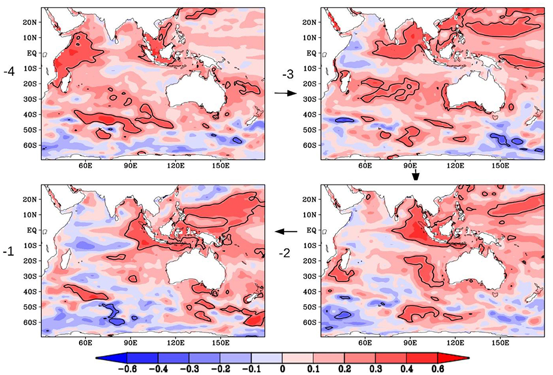
Figure 6. Same as Figure 4 but vertically averaged annually over surface to 100 m depth for the last 4 years leading up to an IOD event. Significant correlations at 95% confidence are shown as contour lines (value at 0.27).

A linear regression analysis carried out using HadISST and ORAS4 ocean temperature datasets (slope value = 0.46) indicates that the Southern Ocean signals at decadal lead explain about 18% of the inter-annual variability of IOD as suggested by a goodness-of-fit measure. To put it in perspective, ENSO, known as the most prominent driver of the Indian summer monsoon interannual variability, explains about 30% of the latter.

The source of decadal predictability for IOD in the MIROC5 and CanCM4 also apparently comes from the Southern Ocean (Supplementary Figure 3). We find statistically significant anomaly correlations between the depth averaged from surface until ~800 m hindcast heat content with the IODMI with the heat content leading at 10–5 years, conforming to our results from the reanalysis. The source of signal is the Southern Ocean for both the models, but the simulated signal path from here to the equatorial Indian Ocean are, however, weaker and remain unclear specifically in the MIROC5 model. However, the signals re-emerge finally 2–3 years before the occurrence of the simulated IOD. The models also do not capture the biennial tendency of the IOD as in observations. Further understanding of other possible factors affecting IOD variability on decadal scales is needed.

Discussion

Our analysis of the CMIP5 decadal retrospective prediction products for the 1960–2011 period shows that two CMIP5 decadal prediction systems exhibit multi-year skill in predicting the IODMI, higher than the 17-month lead skills for the ENSO, a leading climate driver. The physical processes responsible for the skill levels seems to originate in the Southern Ocean up to a decade before emerging in the Indian Ocean, suggesting that this multi-year skill could be extended even further. To our knowledge, this is the first study to show decadal skill in predicting the IOD.

Skill levels for surface fields and, in particular, rainfall, are not statistically indistinguishable from zero. This is in common with long-term predictions of other climate phenomena (Scaife and Smith, 2018) and indicates the relative immaturity of this form of forecasting. It remains a challenge to both improve models and to fully exploit decadal prediction skill. Nevertheless, the potential for long-term planning in both public and private sector organizations that could be facilitated by such skillful predictions is great.

Data Availability Statement

The original contributions presented in the study are included in the article/Supplementary Material, further inquiries can be directed to the corresponding authors.

Author Contributions

FF, KA, and MC formulated the hypothesis and co-wrote the manuscript. FF conducted the analyses. All authors reviewed the final version of the manuscript.

Funding

FF thanks MC and NERC/MoES SAPRISE project (NE/I022841/1) for the travel grant to visit MetOffice, UK. FF acknowledges CSIR for the JRF & SRF fellowship. FF also thanks C T Tejavath for assistance in data processing.

Conflict of Interest

The authors declare that the research was conducted in the absence of any commercial or financial relationships that could be construed as a potential conflict of interest.

Publisher's Note

All claims expressed in this article are solely those of the authors and do not necessarily represent those of their affiliated organizations, or those of the publisher, the editors and the reviewers. Any product that may be evaluated in this article, or claim that may be made by its manufacturer, is not guaranteed or endorsed by the publisher.

Supplementary Material

The Supplementary Material for this article can be found online at: https://www.frontiersin.org/articles/10.3389/fclim.2021.736759/full#supplementary-material

References

Ashok, K., Chan, W.-L., Motoi, T., and Yamagata, T. (2004). Decadal variability of the Indian Ocean dipole. Geophys. Res. Lett. 31:L24207. doi: 10.1029/2004GL021345

CrossRef Full Text | Google Scholar

Ashok, K., Guan, Z., and Yamagata, T. (2003). Influence of the Indian Ocean Dipole on the Australian winter rainfall. Geophys. Res. Lett. 30:1821. doi: 10.1029/2003GL017926

CrossRef Full Text | Google Scholar

Ashok, K., Guan, Z. Y., and Yamagata, T. (2001). Impact of the Indian Ocean Dipole on the relationship between the Indian monsoon rainfall and ENSO. Geophys. Res. Lett. 28, 4499–4450. doi: 10.1029/2001GL013294

CrossRef Full Text | Google Scholar

Ashok, K., and Saji, N. H. (2007). On the impacts of ENSO and Indian Ocean dipole events on sub-regional Indian summer monsoon rainfall. Nat. Hazards. 42, 273–285. doi: 10.1007/s11069-006-9091-0

CrossRef Full Text | Google Scholar

Balmaseda, M. A., Mogensen, K., and Weaver, A. T. (2013). Evaluation of the ECMWF ocean reanalysis system ORAS4. QJR Meteorol. Soc. 139, 1132–1161. doi: 10.1002/qj.2063

CrossRef Full Text | Google Scholar

Barnston, A. G., Tippett, M. K., L'Heureux, M. L., Shuhua, L., and DeWitt, D. G. (2012). Skill of real-time seasonal ENSO model predictions during 2002-11: is our capability increasing? Bull. Amer. Meteor. Soc. 93, 631–651. doi: 10.1175/BAMS-D-11-00111.1

CrossRef Full Text | Google Scholar

Behera, S., Luo, J., and Masson, S. (2005). Paramount impact of the Indian Ocean dipole on the East African short rains: a CGCM study. J. Clim. 18, 4514–4530. doi: 10.1175/JCLI3541.1

CrossRef Full Text | Google Scholar

Behera, S. K., Luo, J. J., Masson, S., Rao, S. A., Sakuma, H., and Yamagata, T. (2006). A CGCM study on the interaction between IOD and ENSO. J. Clim. 19, 1608–1705. doi: 10.1175/JCLI3797.1

CrossRef Full Text | Google Scholar

Boer, G. J., Smith, D., Cassou, C., Doblas-Reyes, F., Danbasoglu, G., Kirtman, B., et al. (2016). The decadal climate prediction project (DCPP) contribution to CMIP6. Geosci. Model. Dev. 9, 3751–3777. doi: 10.5194/gmd-9-3751-2016

CrossRef Full Text | Google Scholar

Cai, W. J., van Rensch, P., Cowan, T., and Hendon, H. H. (2011). Teleconnection pathways of ENSO and the IOD and the mechanisms for impacts on Australian rainfall. J. Climate. 24, 3910–3923. doi: 10.1175/2011JCLI4129.1

CrossRef Full Text | Google Scholar

Chan, S., Behera, S., and Yamagata, T. (2008). Indian Ocean dipole influence on South American rainfall. Geophys. Res. Lett. 35:L14SL12 doi: 10.1029/2008GL034204

CrossRef Full Text | Google Scholar

Delworth, T. L., Broccoli, A. J., Rosati, A., Stouffer, R. J., Balaji, V., Beesley, J. A., et al. (2006). GFDL's CM2 global coupled climate models. Part I: formulation and simulation characteristics. J. Climate. 19, 643–74. doi: 10.1175/JCLI3629.1

CrossRef Full Text | Google Scholar

Doi, T., Behera, S. K., and Yamagata, T. (2016). Improved seasonal prediction using the SINTEX-F2 coupled model. J. Adv. Model. Earth Syst, 8, 1847–1867. doi: 10.1002/2016MS000744

CrossRef Full Text | Google Scholar

Dutta, R., and Maity, R. (2018). Temporal evolution of hydroclimatic teleconnection and long-lead prediction of Indian summer monsoon rainfall using time varying model. Sci. Rep. 8:10778. doi: 10.1038/s41598-018-28972-z

PubMed Abstract | CrossRef Full Text | Google Scholar

Farneti, R. (2017). Modelling interdecadal climate variability and the role of the ocean. Wiley Interdiscip. Rev. Climate Change. 8:e441. doi: 10.1002/wcc.441

CrossRef Full Text | Google Scholar

Gualdi, S., Navarra, A., Guilyardi, E., and Delecluse, P. (2003). Assessment of the tropical Indo-Pacific climate in the SINTEX CGCM. Ann. Geophys. 46, 1–26 doi: 10.4401/ag-3385

CrossRef Full Text | Google Scholar

Ha, K.-J., Chu, J.-E., Lee, J.-Y., and Yun, K.-S. (2017). Interbasin coupling between the tropical Indian and Pacific Ocean on inter annual timescale: observation and CMIP5 reproduction. Clim. Dyn. 48, 459–475. doi: 10.1007/s00382-016-3087-6

CrossRef Full Text | Google Scholar

Hardiman, S. S., Dunstone, N. J., Scaife, A., Smith, D. M., Knight, J. R., Davies, P., et al. (2020). Predictability of European winter 2019/20: Indian Ocean dipole impacts on the NAO. Atmos. Sci. Lett. 21:e1005. doi: 10.1002/asl.1005

CrossRef Full Text | Google Scholar

Iizuka, S., Matsuura, T., and Yamagata, T. (2000). The Indian Ocean SST dipole simulated in a coupled general circulation model. Geophys. Res. Lett. 27, 3369–3372. doi: 10.1029/2000GL011484

CrossRef Full Text | Google Scholar

Izumo, T., Vialard, J., Lengaigne, M., de Boyer Montégut, C., Behera, S., Luo, J. J., et al. (2010). Influence of the state of the Indian Ocean dipole on following year's El Niño. Nat. Geosci. 3, 168–172. doi: 10.1038/ngeo760

CrossRef Full Text | Google Scholar

Jourdain, N. C., Sen Gupta, A., Taschetto, A. S., Ummenhofer, C. C., Moise, A. F., and Ashok, K. (2013). The Indo-Australian monsoon and its relationship to ENSO and IOD in reanalysis data and the CMIP3/CMIP5 simulations. Clim. Dynam. 41, 3073–3102. doi: 10.1007/s00382-013-1676-1

CrossRef Full Text | Google Scholar

Luo, J.-J., Masson, S., Behera, S., and Yamagata, T. (2007). Experimental forecasts of the Indian Ocean dipole using a coupled OAGCM. J. Clim. 20, 2178–2190, doi: 10.1175/JCLI4132.1

CrossRef Full Text | Google Scholar

Luo, J.-J., Zhang, R., Behera, S. K., Masumoto, Y., Jin, F.-F., Lukas, R., et al. (2010). Interaction between El Niño and extreme Indian Ocean dipole. J. Clim. 23, 726–742. doi: 10.1175/2009JCLI3104.1

CrossRef Full Text | Google Scholar

Marathe, S., Terray, P., and Karumuri, A. (2021). Tropical Indian Ocean and ENSO relationships in a changed climate. Clim. Dynam. 56, 3255–3276. doi: 10.1007/s00382-021-05641-y

CrossRef Full Text | Google Scholar

Meehl, G., and Arblaster, J. (2001). The tropospheric biennial oscillation and Indian monsoon rainfall. Geophys Res Lett. 28, 1731–1734. doi: 10.1029/2000GL012283

CrossRef Full Text | Google Scholar

Meehl, G. A., Goddard, L., Boer, G., Burgman, R., Branstator, G., Cassou, C., et al. (2014). Decadal climate prediction an update from the trenches. Bull. Am. Meteorol. Soc. 95, 243–267. doi: 10.1175/BAMS-D-12-00241.1

CrossRef Full Text | Google Scholar

Meehl, G. A., Goddard, L., Murphy, J., Boer, G., Danabasoglu, G., Dixon, K. W., et al. (2009). Can It Be Skillful? Bull. Am. Meteorol. Soc. 90, 1467–1486. doi: 10.1175/2009BAMS2778.1

CrossRef Full Text | Google Scholar

Merryfield, W. J., Lee, W.-S., Boer, G. J., Kharin, V. V., Scinocca, J. F., Flato, G. M., et al. (2013). The Canadian Seasonal to interannual prediction system. Part I: models and initialization. Mon. Wea. Rev. 141, 2910–2945. doi: 10.1175/MWR-D-12-00216.1

CrossRef Full Text | Google Scholar

Murtugudde, R., McCreary, J. P., and Busalacchi, A. J. (2000). Oceanic processes associated with anomalous events in the Indian Ocean with relevance to 1997-98. J. Geophys. Res. 105, 3295–3306. doi: 10.1029/1999JC900294

CrossRef Full Text | Google Scholar

Nauw, J. J., van Aken, H. M., Webb, A., Lutjeharms, J. R. E., and de Ruijter, W. P. M. (2008). Observations of the southern East Madagascar Current and undercurrent and countercurrent system. J. Geophys. Res. 113:C08006. doi: 10.1029/2007JC004639

CrossRef Full Text | Google Scholar

Pal, M., Maity, R., Ratnam, J. V., Nonaka, M., and Behera, S. K. (2020). Long-lead prediction of ENSO modoki index using machine learning algorithms. Sci. Rep. 10:365. doi: 10.1038/s41598-019-57183-3

PubMed Abstract | CrossRef Full Text

Park, J. H., Kug, J. S., Li, T., and Behera, S. K. (2018). Predicting El Niño beyond 1-year lead: effect of western hemisphere warm pool. Sci. Rep. 8:14957. doi: 10.1038/s41598-018-33191-7

PubMed Abstract | CrossRef Full Text

Rayner, N. A., Parker, D. E., Horton, E. B., Folland, C. K., Alexander, L. V., Rowell, D. P., et al. (2003). Global analyses of sea surface temperature, sea ice, and night marine air temperature since the late nineteenth century. J. Geophys. Res. Atmosp. 108:4407. doi: 10.1029/2002JD002670

CrossRef Full Text | Google Scholar

Saji, N. H. (2018). “The Indian Ocean Dipole,” in Oxford Research Encyclopedia of Climate Science, ed H. von Storch (Oxford: Oxford University Press).

Saji, N. H., Goswami, B. N., Vinayachandran, P. N., and Yamagata, T. (1999). A dipole mode in the tropical Indian Ocean. Nature 401, 360–363. doi: 10.1038/43854

PubMed Abstract | CrossRef Full Text | Google Scholar

Saji, N. H., and Yamagata, T. (2003). Possible impacts 209 of Indian Ocean dipole mode events on global climate. Clim. Res. 25:151–169. doi: 10.3354/cr025151

CrossRef Full Text

Scaife, A. A., and Smith, D. (2018). A signal-to-noise paradox in climate science. NPJ Clim. Atmos. Sci. 1:28. doi: 10.1038/s41612-018-0038-4

CrossRef Full Text | Google Scholar

Shinoda, H., Hendon, H., and Alexander, M. A. (2004). Surface and subsurface dipole variability in the Indian Ocean and its relation with ENSO. Deep-Sea Res. 51, 619–635. doi: 10.1016/j.dsr.2004.01.005

CrossRef Full Text | Google Scholar

Smith, D. M., Scaife, A. A., Boer, G. J., Caian, M., Guemas, V., Hawkins, E., et al. (2013). Real-time multi-model decadal climate predictions. Clim. Dyn. 41, 2875–2888. doi: 10.1007/s00382-012-1600-0

CrossRef Full Text | Google Scholar

Sun, Q., Bo, W. U., Zhou, T. J., and Yan, Z. X. (2018). ENSO hindcast skill of the IAP-DecPreS near term climate prediction system: comparison of full field and anomaly initialization. Atmos. Oceanic Sci. Lett. 11, 54–62, doi: 10.1080/16742834.2018.1411753

CrossRef Full Text | Google Scholar

Swapna, P., Roxy, M. K., Aparna, K., Kulkarni, K., Prajeesh, A. G., Ashok, K., et al. (2015). The IITM earth system model: transformation of a seasonal prediction model to a long term climate model. Bull. Am. Meteorol. Soc. 96, 1351–1368. doi: 10.1175/BAMS-D-13-00276.1

CrossRef Full Text | Google Scholar

Tang, Y., Rong-Hua, Z., Ting, L., Wansuo, D., Dejian, Y., Fei, Z., et al. (2018). Progress in ENSO prediction and predictability study. Natl. Sci. Rev. 5, 826–839. doi: 10.1093/nsr/nwy105

CrossRef Full Text | Google Scholar

Tanizaki, C., Tozuka, T., Doi, T., and Yamagata, T. (2017). Relative importance of the processes contributing to the development of SST anomalies in the eastern pole of the Indian Ocean Dipole and its implication for predictability. Clim. Dyn. 49, 1289–1304. doi: 10.1007/s00382-016-3382-2

CrossRef Full Text | Google Scholar

Taylor, K. E., Stouffer, R. J., and Meehl, G. A. (2012). An overview of CMIP5 and the experiment design. Bull. Amer. Meteor. Soc. 93, 485–498. doi: 10.1175/BAMS-D-11-00094.1

CrossRef Full Text | Google Scholar

Tozuka, T., Luo, J. J., Masson, S., and Yamagata, T. (2007). Decadal modulations of the Indian Ocean Dipole in the SINTEX-F1coupled GCM. J. Clim. 20, 2881–2894. doi: 10.1175/JCLI4168.1

CrossRef Full Text | Google Scholar

Trenberth, K. E. (1997). The definition of El Niño. Bull. Am. Met. Soc. 78, 2771–2778. doi: 10.1175/1520-0477(1997)078<2771:TDOENO>2.0.CO;2

CrossRef Full Text | Google Scholar

von Storch, H., and Zwiers, F. W. (1999). Statistical Analysis in Climate Research (Cambridge: Cambridge University Press), 484.

Google Scholar

Wajsowicz, R. C. (2005). Potential predictability of tropical Indian Ocean SST anomalies. Geophys. Res. Lett. 32:L24702. doi: 10.1029/2005GL024169

CrossRef Full Text | Google Scholar

Wang, W., Zhu, X., Wang, C., and Köhl, A. (2014). Deep meridional overturning circulation in the Indian Ocean and its relation to Indian Ocean Dipole. J. Clim. 27, 4508–4520. doi: 10.1175/JCLI-D-13-00472.1

CrossRef Full Text | Google Scholar

Watanabe, M., Suzuki, T., O'ishi, R., Komuro, Y., Watanabe, S., Emori, S., et al. (2010). Improved climate simulation by MIROC5: mean states, variability, and climate sensitivity. J. Clim. 23, 6312–6335. doi: 10.1175/2010JCLI3679.1

CrossRef Full Text | Google Scholar

Webster, P. J., Moore, A., Loschnigg, J., and Leban, M. (1999). Coupled dynamics in the Indian Ocean during 1997-1998. Nature 401, 356–360. doi: 10.1038/43848

PubMed Abstract | CrossRef Full Text

Wu, T., Li, W., Ji, J., Xin, X., Li, L., Wang, Z., et al. (2013). Global carbon budgets simulated by the Beijing climate center climate system model for the last century. J. Geophys. Res. Atmos. 118, 4326–4347. doi: 10.1002/jgrd.50320

CrossRef Full Text | Google Scholar

Yamagata, T., Behera, S., Rao, S., Guan, Z. Y., Ashok, K., and Hameed, S. (2003). Comments on Dipoles, temperature gradients, and tropical climate anomalies. Bull. Am. Meteorol. Soc. 84, 1418–1422. doi: 10.1175/BAMS-84-10-1418

CrossRef Full Text | Google Scholar

Yamagata, T., Behera, S. K., Luo, J.-J., Masson, S., Jury, M., and Rao, S. A. (2004). “Coupled ocean-atmosphere variability in the tropical Indian Ocean,” in: Earth Climate: The Ocean-Atmosphere Interaction, eds. C. Wang, S.-P. Xie, and J. A. Carton (Washington, DC: AGU), 189–212.

Google Scholar

Yeager, S., Karspeck, A., Danabasoglu, G., Tribbia, J., and Teng, H. (2012). A decadal prediction case study: late twentieth century North Atlantic Ocean heat content. J. Clim. 25, 5173–5189. doi: 10.1175/JCLI-D-11-00595.1

CrossRef Full Text | Google Scholar

Zhang, S., Harrison, M. J., Rosati, A., and Wittenberg, A. T. (2007). System design and evaluation of coupled ensemble data assimilation for global oceanic climate studies. Monthly Weather Rev. 135, 3541–3564. doi: 10.1175/MWR3466.1

CrossRef Full Text | Google Scholar