Improvements in Diurnal Cycle and Its Impact on Seasonal Mean by Incorporating COARE Flux Algorithm in CFS

Introduction

Tropical oceans, being the largest storage of heat energy, drive atmospheric circulations that carry energy to other regions of the globe. Generation, strengthening, and termination stages of most of the climate variability in the tropics, such as El Niño–Southern Oscillation (ENSO; Philander, 1985; Neelin et al., 1998), Indian Ocean Dipole (IOD; Saji et al., 1999; Rao et al., 2002), Madden–Julian oscillation (MJO; Madden and Julian, 1971, 1972), and Monsoon Intra-Seasonal Oscillation (MISO; Krishnamurti and Bhalme, 1976; Yasunari, 1980), involve air-sea interaction. Present generation coupled climate models work similarly where the atmosphere and ocean models interact by exchanging heat and momentum fluxes. The surface ocean state (precisely sea surface temperature) acts as the lower boundary condition for the atmospheric component. On the other hand, the turbulent (latent heat, sensible heat, wind stress) and radiative (longwave and shortwave radiations) fluxes from the atmospheric model forces the oceanic model. Therefore, accurately quantifying these exchange variables is required to better understand and represent weather and climate variabilities at different temporal and spatial scales. Blanc (1987) discussed the sources of uncertainties in the computation of surface fluxes in observation and models. Observational uncertainty is due to a lack of data adequacy over various basins, measurement sensors, and platforms limitations, and the existing approximations in different flux computational methods.

In contrast, these uncertainties in the coupled model are due to the inaccurate parameterization of boundary conditions and the propagation of errors to the mean state from observational and reanalysis products. The uncertainty in latent heat flux estimates alone is as high as 80 Wm⁻² (Weare, 1989), and uncertainty among various estimates of fluxes is ~30 Wm⁻². But most of these model errors are due to inaccurate parameterization of sea surface temperature, and turbulent and radiative fluxes exchanged at the air-sea interface. Systematic biases in surface turbulent and heat fluxes are found in atmospheric general circulation models and coupled general circulation models (Wu et al., 2007; Pokhrel et al., 2012; Zhang et al., 2018; Zhou et al., 2020).

In most of the coupled general circulation models, heat and momentum fluxes' parameterization is based on bulk-flux algorithms (Zeng et al., 1998; Chang and Grossman, 1999; Large and Yeager, 2008; Reeves Eyre et al., 2021). The bulk models generally take meteorological parameters at the air-sea interface as input and result in air-sea interactive fluxes as output (Fairall et al., 1996b). One of the crucial parameters required by these bulk models is the air-sea interface temperature, known as skin temperature. However, in most of the coupled models, this temperature is taken as the average temperature in the uppermost layer (called bulk temperature) of the ocean model, typically at a depth of 5 or 10 m. The diurnal variation of skin temperature impacts the diurnal and seasonal variation of air-sea interactive fluxes and modulates various climate variability modes. Two processes contribute to the diurnal variation of skin temperature and its difference from bulk temperature (Fairall et al., 1996a). First, net cooling of the ocean surface occurs due to the outgoing longwave radiation and latent and sensible heat at the air-sea interfacial layer. Second, the establishment of a diurnal warm layer occurs due to the incoming solar radiation. The cumulative effect of diurnal warm layer and cooling can result in intra-daily variability of ocean skin temperature. Observational and modeling studies (Fairall et al., 1996b; Slingo et al., 2003; Shinoda, 2005; Bernie et al., 2007, 2008; Woolnough et al., 2007; Mujumdar et al., 2011; Yan et al., 2021) have reported possible impacts of diurnal skin temperature variability on daily, intra-seasonal, and seasonal mean and variability by modulating ocean-atmospheric parameters such as SST, mixed layer depth, air pressure, humidity, low-level cloud, and convection.

Bulk flux algorithm developed under Tropical Ocean Global Atmosphere (TOGA) Coupled Ocean-Atmosphere Response Experiment (COARE) program known as COARE 3.0 (Fairall et al., 1996b, 2003) flux algorithm is widely used in data analysis and research. The development of the COARE algorithm aimed to limit the estimation errors in the surface fluxes within ±10 Wm⁻². The algorithm has undergone further modifications, improvements, and validation reported by Edson et al. (2013). Most of the reanalysis products, e.g., Objectively Analyzed air-sea Fluxes (OAFlux; Yu et al., 2008), TropFlux (Kumar et al., 2012), and SeaFlux (Curry et al., 2004) related to turbulent surface heat and momentum fluxes are derived using COARE 3.0 flux algorithm. The algorithm is also used to compute fluxes from bulk air-sea parameters measured by moored buoys deployed over global oceans and hence plays a significant role in real-time weather and climate monitoring. One of the major advantages of the COARE 3.0 algorithm is that it takes cool-skin and warm layer effects into consideration (Fairall et al., 1996b). Earlier studies cited above have shown that these effects play an important role in triggering convection. Although the COARE flux algorithm is used in a wide range of reanalysis and observational applications, its usage has not yet extended to present generation coupled models due to its computational complexity. Zeng et al. (1998) and Brunke et al. (2002) have identified that the COARE3.0 algorithm is recognized as one of the least problematic algorithms for computing turbulent fluxes at the ocean surface. Mallick et al. (2020) have shown that implementing the COARE3.0 flux algorithm over the Indian Ocean in Modular Ocean Model v3.0 had demonstrated significant improvements in SST representation by reducing the errors in simulated SSTs by 5–40% in the Bay of Bengal. In addition, they have also shown that the upper ocean temperature profiles have also improved by reducing the biases by 10–40%. Cool Skin Effect (known as the temperature difference across the skin layer of the surface layer) impacts the computation of latent heat. It reduces the overestimation by ~9% in the south China Sea (Zhang et al., 2020). Misra et al. (2008) have shown that the presence of skin temperature can reduce the cold tongue bias over equatorial Pacific.

Under the monsoon mission (Rao et al., 2019), the Indian Institute of Tropical Meteorology (IITM) has focused on improving the seasonal forecasting capability of India using Climate Forecast System version 2 (CFSv2) tuned for monsoon prediction. The model is reported to have large seasonal mean biases in SST (George et al., 2016; KBRR et al., 2020), mixed layer depth, surface fluxes (Wu et al., 2007; Pokhrel et al., 2012), and precipitation (Ramu et al., 2016; Krishna et al., 2019) which hinders its prediction capability. Simulation of relations between Rainfall-SST and latent heat-SST are also not realistic in CFSv2, thereby creating an improper representation of global teleconnections such as ENSO-monsoon and IOD-monsoon relations (Chattopadhyay et al., 2016; Pillai et al., 2017; Krishna et al., 2019). The problems related to the simulation of the diurnal phase and amplitude of precipitation over Indian landmass and adjoining oceans are also reported for this model (Ganai et al., 2016). Motivated by the earlier mentioned studies and to reduce these systematic biases in CFSv2, this study is an attempt to introduce COARE3.0 based skin temperature and flux parameterization in the CFSv2 model. The study documents the impact of the implementation of skin temperature parameterization along with a revised flux scheme on the diurnal and seasonal scale mean biases, variability, and prediction skill of various ocean-atmosphere parameters with the help of coupled model simulations. Section-Data, Model, and Methodology describes the incorporation of COARE3.0 into CFSv2 and sources of different observation/reanalysis datasets used in the present study. Section-Results and Discussion presents the results by comparing the hindcast simulations in CFSv2 with default and revised flux and skin temperature parameterization, followed by a summary and future scope of the present study in section-Summary and Discussion.

Data, Model, and Methodology

In most of the coupled models, the air-sea interactive fluxes are computed using bulk flux algorithms. Bulk methods assume that the turbulent fluxes are related to differences in wind speed, temperature, and specific humidity between the air-sea interface and one level in the atmosphere. The bulk algorithms are used in place of eddy correlation method when high resolution (spatial or temporal) boundary layer data is not available. The various fluxes are computed as listed in the following equations.

$\begin{array}{llll}\text{Latent heat flux},Q_{lat}& =& {\rho }_a{L}_e{C}_{e}S(q_s-q),& (1)\end{array}$

$\begin{array}{llll}\text{Sensible heat flux},Q_{sen}& =& {\rho }_a{c}_{pa}{C}_{h}S(T_s-T),& (2)\end{array}$

$\begin{array}{llll}\text{Wind stress},\tau & =& {\rho }_a{C}_{d}S(u_s-u),& (3)\end{array}$

Where the bulk transfer coefficients for latent heat, sensible heat, and stress are C_e,C_h, and C_d respectively. S is the average value of the wind speed relative to the sea surface current, q_s is the interfacial value of the water vapor mixing ratio, and u_s is the surface current. Similarly, q, u, and T are water vapor mixing ratio, wind speed, and air temperature at the lowest level of atmosphere. q_s is computed from saturation specific humidity for pure water at the SST. ρ_ais the air density, L_e is the latent heat of vaporization, and c_pais the specific humidity of air at constant pressure.

Two sets of hindcast simulations are generated with a common study period of 1981–2017. These simulations have been carried out with CFSv2 at T126 (~100 Km) atmospheric horizontal resolution, which was initially adapted from NCEP. The brief details about various components of the model are summarized in Table 1. The first set of hindcasts (will be denoted as CTL run hereafter) are with the default setup of CFSv2 as described by Saha et al. (2014). Therefore, in the CTL run, the turbulent fluxes at the ocean-atmosphere boundary are computed following Large and Yeager (2008) (National Center for Atmospheric Research, NCAR algorithm). The atmosphere (time step =10 min) and ocean model (time step =30 min) are coupled at every 30 min of the model time step. The meteorological parameters like wind, air temperature, humidity, and pressure at the bottom of the atmospheric model are used as forcing for the ocean model. The oceanic model's SST (5 m temperature) acts as a lower boundary forcing for the atmospheric component. Hence, the CTL run lacks corrections for diurnal skin temperature variations. The second set of hindcasts is by implementing COARE3.0, where turbulent surface flux, diurnal cool skin, and warm layer temperature corrections are computed by following Fairall et al. (1996a,b, 2003). Thus, the skin temperature computed acts as the boundary forcing for the atmospheric model instead of 5 m bulk ocean temperature. Also, the COARE3.0 computed turbulent fluxes at the air-sea interface replace the fluxes based on the NCAR algorithm. Therefore, in SEN run the flux scheme is totally replaced by COARE3.0.

TABLE 1

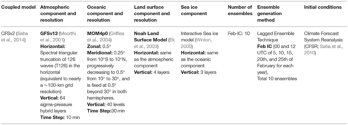
Table 1. Description about model grid, resolution, and initialization of different components of CFSv2.

The above-mentioned basic equations for flux computation remain similar in both the algorithms. However, the two flux schemes differ from each other in the way the transfer coefficients, roughness lengths are computed, and the way is defined in respective flux scheme. A brief difference between the flux schemes of CTL and SEN run is represented in Table 2. For a detailed intercomparison between NCAR and COARE, readers are encouraged to refer to Fairall et al. (1996b), Zeng et al. (1998), and Large and Yeager (2004, 2008). The turbulent fluxes exchanged at the air-sea interface depend on the formulation of drag coefficients (or roughness lengths), stability functions, and reduction of surface humidity due to salinity. The stability function in the NCAR algorithm is based on two regimes, namely stable and unstable, and the roughness length and the drag coefficients are computed according to these stability regimes. The COARE3.0 algorithm is based on three stability regimes, namely stable, weakly stable, and strongly unstable, and the roughness lengths are a continuous function of wind. The COARE algorithm also includes a gustiness factor in low wind conditions to account for increased fluxes. The surface-specific humidity in the NCAR algorithm is a function of the only temperature, whereas that in the COARE algorithm is a function of temperature and pressure. Both the algorithms consider the reduction of humidity due to ocean salinity.

TABLE 2

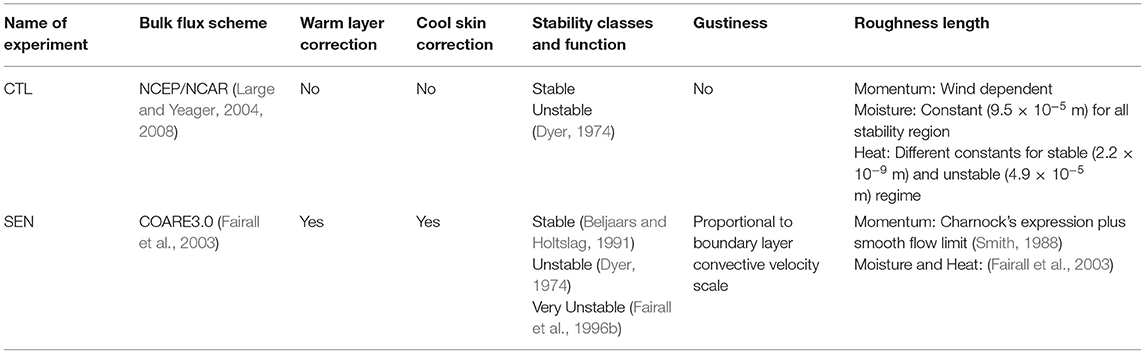
Table 2. Description of difference between the bulk flux algorithms in CTL and SEN simulations.

The skin temperature computation is an inherent part of COARE3.0 algorithm and it is not part of a prior version of CFSv2 (i.e., the CTL run). In prior versions of CFSv2, the air-sea interactive fluxes are computed based on bulk ocean temperature instead of skin temperature. Hence, CTL run misses out the diurnal variability of surface ocean and its impact on the atmosphere. The skin temperature is computed from the bulk ocean temperature by incorporating two physical corrections: (1) The diurnal warm layer correction and (2) The diurnal cool skin temperature correction. Both the cool skin and warm layer temperature corrections depend not only on bulk ocean temperature but also on the accumulated/instantaneous turbulent fluxes on the air-sea boundary. The skin temperature parameterization is given as:

$\begin{array}{ll}{T}_{skin}=T_{Bulk}+\Delta T_{warm}(z_r)-\Delta T_{cool},& (4)\end{array}$

Where T_skin is the skin temperature estimated from bulk ocean temperature T_Bulk, warm layer correction ΔT_warm, and cool skin correction ΔT_cool. The warm layer correction at a depth z_r (where the bulk temperature is measured/modeled) depends on the time averaged/accumulated net radiation (I_S) and momentum(I_τ) at the surface and is given by

$\begin{array}{ll}\Delta T_{warm}(z_r)=\frac{\alpha g{\left(\frac{I_s}{\rho c_p}\right)}^{\frac{1}{2}}}{R_{ic}{I}_{\tau }^2}{z}_r,& (5)\end{array}$

where R_ic =0.65 is the bulk Richardson number, g is the acceleration due to gravity, α is the thermal expansion coefficient, ρ is the density, and c_p is the specific heat of water. The cool skin temperature depends on the net radiative cooling Q_net due to outgoing latent heat, sensible heat, long wave radiation, and nest incoming solar radiation (δS_c) and is given by

$\begin{array}{ll}\Delta T_{cool}=(Q_{net}-\delta S_c)\delta /k,& (6)\end{array}$

where δ is the molecular sublayer where cooling is confined and k is the thermal conductivity of water.

For the analysis of seasonal mean biases and prediction skills, the hindcast simulations are set for daily output frequency and are integrated for 9 months, starting with February's initial conditions. The 10 ensemble members are generated using lagged ensemble generation technique as mentioned in Table 1. The analysis of diurnal variations is carried out for 1998–2008, and the model output frequency is set to 3 h for these simulations. All the analyses discussed in this study focus on boreal summer unless stated explicitly. For diurnal scale analysis, satellite-derived SST data is taken from SeaFlux (Curry et al., 2004), available at a horizontal resolution of 0.25° and a temporal resolution of 1-h. Diurnal analysis involving precipitation rate uses Tropical Rainfall Measuring Mission (TRMM; Huffman et al., 2010) data available at 0.25° horizontal and 3-h temporal resolution. Hourly ocean sub-surface temperature data is obtained from tropical moored buoy observing systems: TAO/TRITON and RAMA at several Pacific and Indian Ocean locations. The moored buoy observations are used explicitly for model validation. Mixed layer depth (MLD) is computed using a threshold temperature criterion from subsurface temperature observation/model data. Following Montégut et al. (2004), the MLD is defined as a depth where the ocean temperature decreases by 0.2°C from the surface temperature. Monthly mean rainfall and SST from Global Precipitation Climatology Project version 2.3 (GPCP v2.3; (Adler et al., 2018) and Extended Reconstructed Sea Surface Temperature, Version 5 (ERSSTv5; Huang et al., 2017) are taken, and both are available globally at 2.5°×2.5° horizontal resolution. For Latent heat, sensible heat, and wind stress TropFlux (Kumar et al., 2012) data is considered and is available at 1.0°×1.0° horizontal resolution in the tropics (i.e., from 30°S to 30°N) only. Descriptions about the various datasets used in the present study are summarized in Supplementary Table 1.

Results and Discussion

Impact at Diurnal Scale

Diurnal SSTs

As mentioned in the previous section, one of the major differences between CTL and SEN simulation is the presence of cool skin and warm layer temperature parameterizations in the latter one. The impact of these parameterizations on intra-daily ocean temperature variability can be seen in Figure 1, where the climatological diurnal range of SST (dSST=maximum-minimum during a 24-h cycle) is plotted during monsoon season (JJAS). Figure 1A shows the mean dSST in the satellite-derived SeaFlux observation. During JJAS, a higher magnitude of dSST in the northern hemisphere can be seen due to the seasonality of solar insolation and winds. The seasonal patterns are consistent with Stuart-Menteth et al. (2003) and Kawai and Wada (2007). Seasonal mean dSST is higher near the western Pacific, western coast of North America, northern Atlantic, equatorial eastern Pacific, and the equatorial Indian Ocean. The equatorial west Pacific and western coast of North America have the largest dSST, ranging up to 1°C. The diurnal range in SST is significantly weaker in the CTL run, as shown in Figure 1B, where the seasonal mean maximum dSST reaches 0.35°C. However, the locations of maximum dSST are comparable to observation except over the northern Pacific Ocean. With the inclusion of diurnal skin temperature parameterization, the diurnal SST is significantly improved over by 0.2–0.3°C over the tropical Indian Ocean and by 0.4–0.5°C over the north Pacific and Atlantic Oceans. The magnitude and locations of maximum dSST are comparable to the observation. In the sensitivity run, dSST has a higher magnitude over the equatorial and northern Pacific and Atlantic Oceans (i.e., the summer hemisphere). Over the Indian Ocean, a higher magnitude of dSST can be seen over the central equatorial Indian Ocean and near islands' coasts at the eastern Indian Ocean. The magnitude of dSST in the SEN run is still smaller compared to the observed dSST. However, significant improvements are noticed compared to the CTL run. Implementation of cool skin and warm layer corrections (Fairall et al., 1996a) to the bulk ocean temperature (which is at 5 m in the model) as a part of the COARE3.0 algorithm helped in improving the diurnal warming/cooling of the surface ocean, thereby increasing the diurnal range of ocean temperature. Similar improvements in dSST in SEN are seen during other seasons (figure not shown).

FIGURE 1

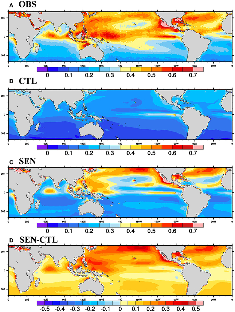
Figure 1. Seasonal (JJAS) Mean diurnal range of SST (dSST = maximum-minimum during 24-h cycle in °C) from (A) observation (SEA-FLUX), (B) CTL, (C) SEN run, and (D) SEN minus CTL for the period 1998–2007.

To further validate against in-situ observations, a comparison of local diurnal cycles of SST is carried out at various locations over the Bay of Bengal and the Pacific Ocean. These locations are selected based on their importance toward the Indian summer monsoon and high-frequency availability during the study period. Lows and depressions are important rain-bearing systems for the Indian monsoon that preferably originate over the Bay of Bengal (BoB) and propagate toward the Indian landmass. Studies have suggested that the diurnal scale variability of SST over BoB is small (Bellenger and Duvel, 2009) due to persistent strong monsoon winds and high cloud cover. In contrast, studies like Mujumdar et al. (2011) suggested that the diurnal variability in SST over BoB can be as large as the amplitude of intraseasonal variability. Therefore, it is essential to discuss the improvement in diurnal scale SST variations over BoB. The diurnal cycle of SST over the western Pacific is also discussed because dSST is significant over the western Pacific, as shown in Figure 1A. The model simulated and observed intra-daily SST variation can be seen from Supplementary Figures 1A–C, where SSTs at various locations over the BoB and western Pacific Oceans are plotted w.r.t local solar time (LST). In the observation, the SST has a minimum and maximum value at around 7 and 16 h of LST, respectively. The timings of minima and maxima are delayed in the CTL run, with minima and maxima occurring at about 10 and 19 h of LST, respectively. But in the SEN run, the timings of maxima and minima are significantly improved and agree with the observation. The amplitude of diurnal SST at these locations is also underestimated in the CTL run and improved in SEN run compared to OBS. Therefore, the implementation of COARE in CFSv2 improves the timing and amplitude of diurnal minima and maxima. Similar improvements are seen over other parts of the globe and during other seasons as well.

Diurnal MLD

To see whether the modification in ocean skin temperature variability and amplitude is reflected in the mixed layer processes or not, we further analyze the diurnal range of MLD (dMLD). dMLD is defined similarly to dSST, discussed earlier. Due to the unavailability of intra-daily MLD observations/reanalysis products, the comparison of spatial patterns of dMLD is restricted to model simulations. Figure 2 shows the dMLD simulated by both the simulations along with the difference between them. The diurnal range in both the simulations is relatively larger over the central and eastern equatorial Pacific, equatorial Atlantic, and western Indian oceans. The same diurnal range in precipitation is minor over the northern subtropical oceans, Indian Ocean, and BoB. A comparison of two simulations suggested that the dMLD has increased in SEN run compared to CTL run over most tropical oceans. The increase in dMLD is prominent over the western and central tropical Pacific and the eastern Indian oceans. Regions like subtropical oceans and the Arabian Sea have experienced a slight reduction in dMLD. Therefore, the skin temperature correction and revised flux parameterization have impacted the surface ocean and modulated the diurnal mixing and upper ocean heat content. Over the tropical Pacific and the Indian Ocean, where moored buoy data is available at the higher temporal resolution, the comparison of MLD variability w.r.t. LST is carried out (Supplementary Figures 1D–F). During the early hours of the day, the observed MLD is more profound due to enhanced mixing because of radiative heat loss. The depth increases gradually up to 10 LST, and then a shallow mixed layer is formed during local afternoon hours due to the increased solar insolation in the upper surface layer, creating stable stratification. Again, during sunset, mixed layer depth increases with increased heat loss. Both the model simulation captures the intra-daily phases of MLD quite well with significant underestimation in magnitude. However, the comparison of both simulations suggests a more considerable underestimation of mixing in CTL run during nighttime compared to the SEN run. The amplitude difference between early morning deep MLD and afternoon shallow MLD is significantly low in CTL run compared to SEN run. The enhancement in MLD at the diurnal scale shown in Supplementary Figure 1 is also supported by the earlier discussion of Figure 2, where the SEN run showed an increased dMLD over most tropical ocean basins. Therefore, the impact of the skin temperature and revised flux scheme is not limited to the surface ocean but is also seen at the upper ocean mixed layer processes at a diurnal scale.

FIGURE 2

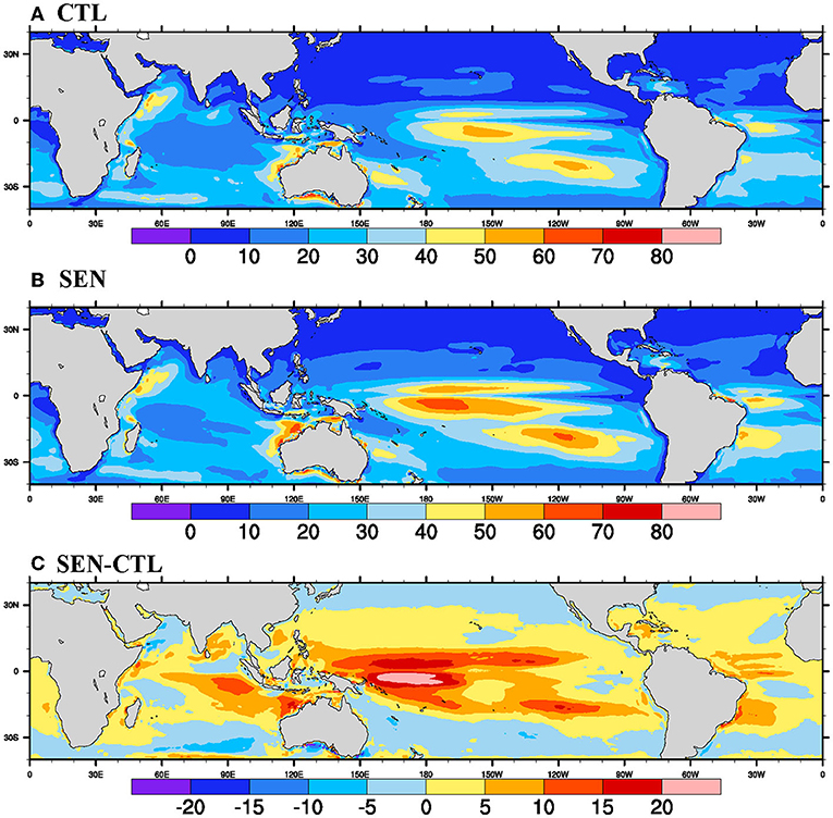
Figure 2. Seasonal (JJAS) Mean diurnal range of MLD (dMLD = maximum-minimum during 24-h cycle in m) from (A) CTL, (B) SEN run, and (C) SEN minus CTL for the period 1998–2007.

Diurnal Precipitation

Diurnal variation of SST is driven by solar heating and is strongly modulated by meteorological conditions such as wind speed, air-sea humidity difference etc. [Kawai and Wada (2007) and the references therein]. Relatively few modeling studies report the significant impact of resolving diurnal scale SST on the atmosphere. Through coupled model experiments, Dai and Trenberth (2004) have shown that the lack of diurnal variation of SST can adversely impact the diurnal cycles of air temperature, air pressure, and precipitation. Similarly, Li et al. (2001) have shown that the presence of the diurnal cycle of SST as forcing to the atmospheric model helps better simulate the intraseasonal oscillations in precipitation and surface fluxes. Chen and Houze (1997) have shown that the diurnal heating of the sea surface is essential for convection over the western Pacific warm pool region. The diurnal SST rise during the suppressed convection phase can lead to the formation of shallow convective clouds (Chen and Houze, 1997; Sui et al., 1997; Johnson et al., 1999; Slingo et al., 2003). By moistening the free troposphere, the shallow clouds generate favorable conditions for the next active phase with enhanced deep convection. Clayson and Chen (2002) suggested that the atmospheric model is sensitive to skin effect, diurnal variations in SST, and choice of bulk flux algorithm.

This section addresses the impact of diurnal SST variation on diurnal scale precipitation during the southwest monsoon period. The seasonal mean diurnal range of precipitation (dprate) is defined as the long-term seasonal average of maximum minus minimum rainfall value during a 24-h cycle at each grid point. Figure 3 shows the dprate for observation (TRMM) and two model simulations (with default NCAR and COARE3.0 algorithm). In observations, the diurnal range in rainfall is significant over the equatorial oceans and landmasses. A higher magnitude of dprate is observed over the western Pacific warm pool regions, the east and central Indian Ocean, and northern BoB. Over the western Pacific warm pool, the diurnal range is as high as 2.25 mm/h. The horseshoe pattern in dprate over the Indian Ocean and continent is evident in Figure 3A, similar to the seasonal mean rainfall pattern. A similar pattern in dprate is also reported by Ganai et al. (2016) and Kim et al. (2019). The eastern Indian Ocean has a dprate of the order 2.25–2.75 mm/h. In addition to the eastern Indian Ocean, a secondary region of maxima is found over northern BoB, which extends toward eastern and northeastern Indian landmass. Over the Indian landmass, dprate is higher over the western Ghats, eastern coasts, north-east, and foothills of Himalaya, similar to the seasonal mean rainfall pattern during the southwest monsoon.

FIGURE 3

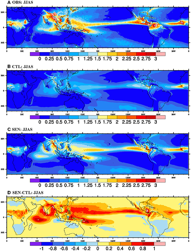
Figure 3. Seasonal (JJAS) Mean diurnal range of prate (dPRATE = maximum-minimum during 24-h cycle in mm/h) from (A) observation (TRMM), (B) CTL, (C) SEN run, and (D) SEN minus CTL for the period 1998–2007.

The amplitude of the diurnal range is significantly lower in CTL (Figure 3B) run throughout the global oceans and landmasses. However, the pattern of maxima and minima agree with the observation. The amplitude of dprate over the Indian Ocean and landmass is not well-represented in the absence of appropriate diurnal variation of skin temperature. Implementing diurnal skin temperature and flux parameterization in the COARE algorithm results in amplified dprate (Figure 3C) throughout the global tropical oceans and landmasses. The amplitude of dprate is closer to observation over the eastern Indian Ocean, north BoB, western Ghats, and the foothills of the Himalaya. However, the amplitude of dprate is still underestimated in many parts of the global oceans and specifically over landmasses such as South America, Africa, and India. The enhancement in dprate is as large as 0.5–1.0 mm/hour in SEN run compared to CTL run for most tropical oceans and Indian landmass regions during the southwest monsoon season, as shown in the difference plot (Figure 3D). The enhancement in diurnal precipitation is due to the changes in winds and mixed layer at the lower atmosphere, and shallow cumulus convection related to diurnal SST variation as suggested by Slingo et al. (2003) and Kawai and Wada (2007). Bellenger et al. (2010) have shown that during the episodes of large diurnal warm layer formation, convection's diurnal cycle is characteristically different from that during the episodes of no diurnal warm layer formation. Episodes with no diurnal warm layer are accompanied by a convection maximum in the early morning, whereas during episodes with a higher, stronger warm layer, convection peaks around noon to afternoon. The characteristically different behavior of convection is also primarily affected by the surface flux changes and convective inhibition energy (CIN)/convective available potential energy (CAPE).

Further analysis is carried out to see whether the revised flux and skin temperature parameterization impact the time of peak diurnal rainfall activity during the southwest monsoon season. Previous studies (Slingo et al., 2003; Ganai et al., 2016) have shown an interesting diurnal signal related to the convective anomaly spreading from India to the adjacent BoB. Harmonic analysis of the diurnal cycle of rainfall is carried out to get the diurnal phase information (in coordinated universal time; UTC) over BoB and Indian landmass and is plotted in Supplementary Figure 2. Similar to the study of Slingo et al. (2003), constant phase lines spread out from the east coast of India into the BoB in observation as well as both the model simulations. Over the oceanic part, both the models could capture the phase propagation reasonably well, whereas over the Indian landmass, the diurnal peak rainfall appears to be earlier (by 2 h) than observations. There is a slight improvement in the simulated time of peak diurnal rainfall over central and north-western Indian landmass in the SEN run compared to the CTL run. In addition to diurnal skin temperature scheme, proper parameterization of topographic influence (Mao and Wu, 2012), land-sea breeze (Yang and Slingo, 2001), the response of convection to gravity waves (Slingo et al., 2003), etc. are needed to improve diurnal phase of convective anomalies in general circulation models.

Studies have suggested that the diurnal variability of surface and subsurface ocean impacts diurnal atmospheric properties and can modulate the intraseasonal and seasonal ocean and atmospheric processes. Observational studies (Mujumdar et al., 2011; Yan et al., 2021) have shown rectification of intraseasonal SST by diurnal variations of SST over most tropical oceans. Through coupled model experiments, Bernie et al. (2007, 2008) have shown that the rectification of daily-mean SST by the diurnal variability of SST can increase the long-term-mean SST by 0.2°-0.3°C and an improvement in the mean precipitation simulated by the model. They have also reported the possibility of enhanced equatorial upwelling because of the modulation of equatorial current by diurnal SSTs. Intra-daily SST variations can modulate the intra-daily mixed layer depth and impact intraseasonal SST and mixed layer processes (Bernie et al., 2005; Shinoda, 2005; Kawai and Wada, 2007; Woolnough et al., 2007; Thushara and Vinayachandran, 2014). Chen and Houze (1997), Li et al. (2001), Slingo et al. (2003), and Bellenger et al. (2010) have reported enhanced precipitation due to triggering more shallow convection/clouds by diurnal skin temperature warming. Brunke et al. (2008) have shown seasonal mean changes in winds, precipitation, and surface fluxes by including skin temperature parameterizations in the standalone atmospheric model. Therefore, further analysis is carried out to check how the diurnal scale skin temperature and flux parameterization can impact the seasonal mean state of the ocean, atmosphere, and interface.

Impact at Seasonal Scale

Impact on Heat and Momentum Fluxes

The CTL and SEN run differs in the parameterization of skin temperature, turbulent surface heat, momentum, and radiative fluxes. These fluxes act as forcing for the ocean model, whereas SST/skin temperature forces the atmospheric model. The exchange of fluxes and SSTs occurs at every coupling time step between the ocean and atmosphere. The impact of the coupling strategies of surface temperature and fluxes on seasonal mean biases of various ocean and atmospheric parameters is discussed in this section. The seasonal mean turbulent heat, i.e., latent heat and sensible heat and momentum fluxes from CTL and SEN runs, is compared in Figures 4–6, respectively. The seasonal (JJAS) mean biases of surface latent heat are shown in Figure 4 for both the runs and the difference between them. The latent heat is overestimated throughout the global ocean in both runs, similar to the earlier studies by Wu et al. (2007) and Pokhrel et al. (2012). Similar overestimation of latent heat flux is also seen in atmospheric general circulation models, as discussed in Zhou et al. (2020). Over the Pacific Ocean, the magnitude of biases is largest over North and South America's coasts and at 10°S of the eastern and western Pacific Ocean. Over the Indian Ocean, considerable overestimation is noticed along with the monsoon south-westerly flows, Arabian Sea, Bay of Bengal, and at 10°S of the central Indian Ocean. Over these regions, the LHF biases are as significant as 80–100 W/m². The comparison suggests that the magnitude of LHF bias in the SEN run is significantly reduced compared to the CTL run. In the SEN run, the overestimation is reduced by 15–30 W/m² over the north-central and the south-eastern Indian Ocean. Over the tropical Pacific and the Atlantic Ocean, the magnitude of improvement in bias is of the order of 5–15 W/m². The model simulation's relative contributions of air-sea humidity difference (delQ) and wind speed toward the difference in latent heat flux between the model simulations are computed and plotted in Supplementary Figure 3. The difference in latent heat is represented as

$\begin{array}{ll}LH{F}^{\prime }=\rho C_e(W^{\prime }\overline{\Delta Q}+\bar{W}\Delta Q^{\prime }+W^{\prime }\Delta Q^{\prime }+\overline{W^{\prime }\Delta Q^{\prime }})& (7)\end{array}$

FIGURE 4

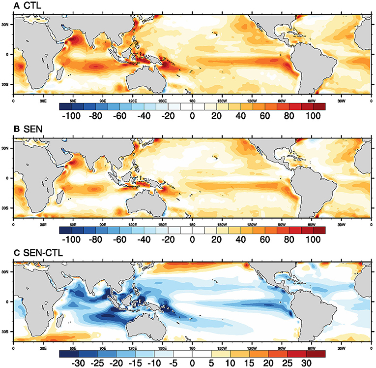
Figure 4. Seasonal (JJAS) mean bias in Latent Heat Flux (LHF in Wm-1) in (A) CTL run, (B) SEN run, and (C) SEN-CTL for the period of 1981–2017.

Where LHF is latent heat, W is wind speed, ΔQ is the air-sea humidity difference, ρ is the surface air density, and C_e is the bulk transfer coefficient. The prime represents the difference, and the overbar represents the climatology of various parameters in the control run. We have taken CTL simulation as a reference for this computation, instead of the observation used by Pokhrel et al. (2012) and Zhou et al. (2020) as we are interested in the changes between the two simulations. The first and second term of equation-1 represents the wind and delQ contributions respectively whereas the last two terms on the right-hand side of Equation 7 have negligible contributions. Wind speed's relative contribution is more over the Indian Ocean (except the eastern Indian Ocean) toward the observed reduction in latent heat fluxes in SEN run compared to the CTL run. Similarly, over the equatorial Pacific Ocean, the contribution of delQ is more toward observed latent heat flux differences between the model simulations. Therefore, the reduction in latent heat flux is influenced by changes in delQ and wind speed, and their contributions differ from region to region. Studies like Bonino et al. (2020) have shown that skin temperature parameterization can also reduce the evaporation and hence turbulent heat fluxes significantly.

Another component of turbulent heat flux is sensible heat flux. During the boreal summer over the tropical latitudes, the contribution of sensible heat flux (SHF) toward the variability of net heat flux and SST is smaller than latent heat flux. The magnitude of the seasonal mean of SHF is also smaller compared to other surface fluxes like LHF and longwave radiation. The seasonal mean biases (Figure 5) of SHF in both the runs are smaller and not significant compared to the biases in LHF, and hence the difference between the two runs is also smaller. Only marginal reduction of SHF in SEN run can be seen over the south-eastern Indian Ocean, subtropical Pacific, and the Indian Ocean. Surface momentum flux forces the oceanic model, which drives the ocean circulation and impacts the ocean-atmosphere interface. Bias in surface momentum flux depends on the parameterization of momentum drag coefficients and, hence, wind stress formulation. A brief on differences between the NCAR and COARE3.0 algorithms is presented earlier in the “data, model, and methodology” section. Detailed discussion on the formulation of drag coefficients and wind stress in the NCAR and COARE3.0 can be found in Fairall et al. (2003) and Large and Yeager (2004, 2008), but is not the prime objective of the present study. The bias in surface stress for both simulations is shown in Figure 6, where the magnitude of wind stress bias is represented in color shading and horizontal vector as arrows. In the CTL run magnitude of wind, stress is overestimated over most of the global oceans, with the Indian Ocean dominated by the southerly component of the stress bias whereas the Pacific Ocean is dominated by zonal wind stress bias. Over the Southern Ocean, the stress is primarily overestimated in the CTL run. In the SEN run, the overestimation of easterly zonal wind stress over the subtropical North Pacific Ocean is reduced significantly. Also, the surface stress bias over the Southern Ocean is improved considerably. Over the southern Indian Ocean between 20°S and 30°S, there is a notable change of bias in stress between the CTL and SEN runs. The difference (Figure 6C) in seasonal mean surface stress between the two runs suggests an increase in wind stress near the eastern and western Indian Ocean coasts, north and south of the equatorial Indian Ocean. Over the Pacific Ocean, there is an increase in zonal stress on both sides of the equator. The results indicate significant modification of surface momentum flux over the global tropical oceans because of changing the bulk flux parameterization schemes.

FIGURE 5

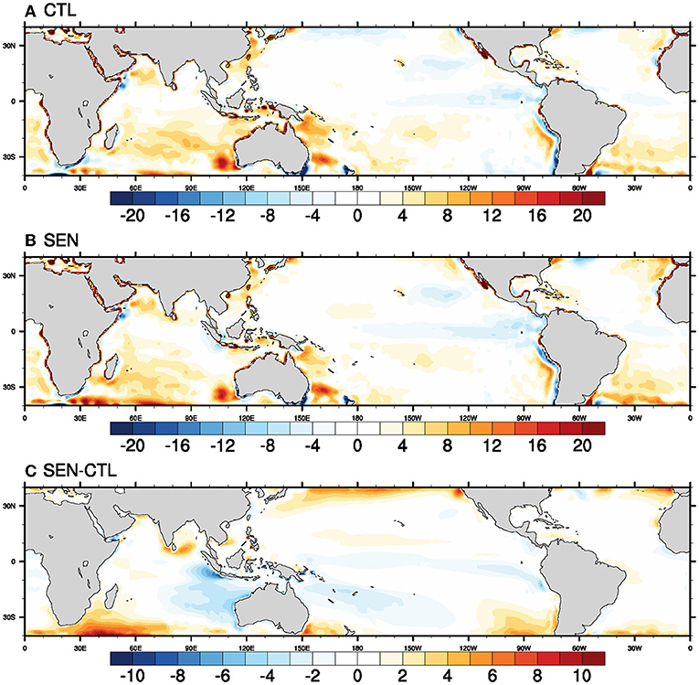
Figure 5. Seasonal (JJAS) mean bias in Sensible Heat Flux (SHF in Wm-2) in (A) CTL run, (B) SEN run, and (C) SEN-CTL for the period of 1981–2017.

FIGURE 6

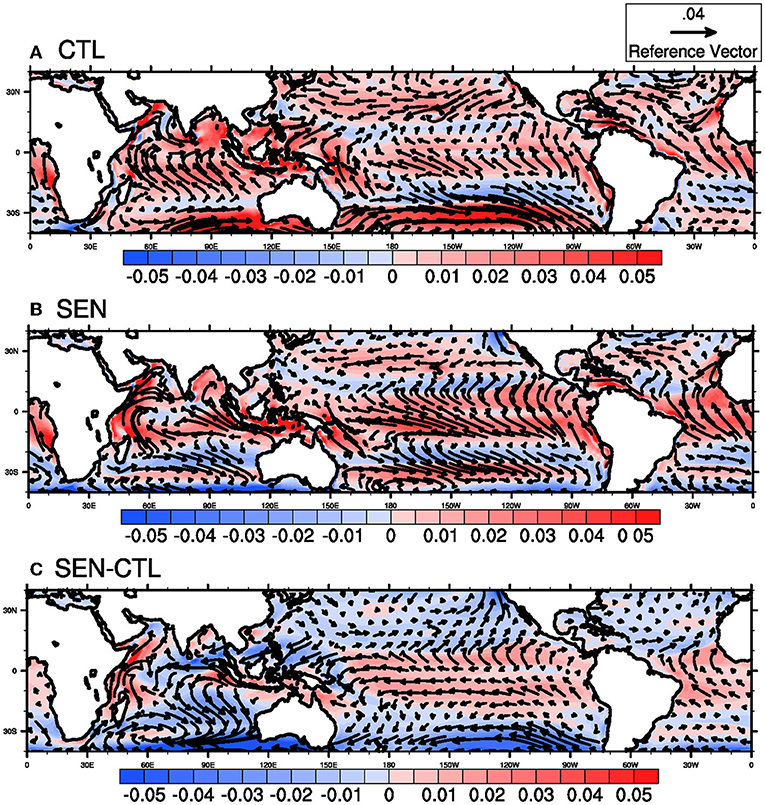
Figure 6. Seasonal (JJAS) mean bias in momentum flux (stress in m2s-2) in (A) CTL run, (B) SEN run, and (C) SEN-CTL for the period of 1981–2017. The colored shading represents the magnitude of stress and zonal and meridional components are represented as vectors.

Impact on Mixing and Ocean Temperature

Earlier sections Diurnal SSTs and Diurnal MLD discussed how the lack of diurnal scale skin temperature parameterization has adversely impacted the diurnal mixed layer representation in the CTL run. Similarly, the previous section suggested how COARE3.0 bulk flux parameterization helped improve the surface flux biases in the CFSv2. This section discusses the impact of better representation of seasonal mean flux and diurnal skin temperature and mixed layer processes on seasonal mean MLD biases. The enhanced mixing caused in the SEN run can be seen from Figure 7, where MLD bias is plotted for two simulations along with the differences between them. The bias in CTL plotted in Figure 7A shows significant shallow MLD bias over the tropical western and central Pacific Ocean, tropical Atlantic Ocean, and the northern Indian Ocean. On the other hand, the mixing is overestimated in the Southern Ocean. In the SEN run (Figure 7B), the shallower MLD bias is significantly reduced over the equatorial and southern Pacific, Atlantic, and Indian. The overestimation of MLD over the Southern Ocean is also reduced considerably. Therefore, the seasonal mean MLD has increased in the SEN run, indicating enhanced mixing at seasonal time scales compared to the CTL run. The difference in the pattern of simulated seasonal mean MLD is similar to the difference between the diurnal range of MLD simulated in both the simulations, as discussed in section Diurnal MLD. The modifications/improvements in diurnal scale skin temperature, fluxes, and mixing are translated into alterations in seasonal scale mixed layer properties. Likewise, the increase in zonal surface stress over the equatorial Pacific and meridional stress over the eastern and western Indian Ocean favor enhanced upwelling. Also, the enhanced stress and the reduced stratification over the surface ocean favor more mixing at those locations.

FIGURE 7

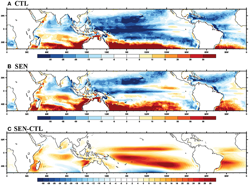
Figure 7. Seasonal (JJAS) mean bias in mixed layer depth (MLD in m) of the ocean in (A) CTL run, (B) SEN run, and (C) SEN-CTL for the period of 1981–2017.

The cumulative effect of seasonal mean surface fluxes and mixing impacts the ocean surface temperature. Seasonal mean biases in 5-m ocean temperature for the CTL and SEN hindcast runs are shown in Figures 8A,B, respectively. Both the models have cold SST bias over most of the global tropical oceans. The significantly warm SST bias over the western coasts of North and South America in both runs is common in most of the coupled global models (Pillai et al., 2018; Krishna et al., 2019) and is due to the misrepresentation of stratus cloud in the atmospheric component (Zheng et al., 2011) of the models as mentioned earlier. Comparison of SST biases (Figure 8C) over the Pacific Ocean suggests that cold SST bias over the equatorial Pacific is enhanced whereas, over the subtropical Pacific, it is reduced in the SEN run compared to the CTL run. Over the tropical Indian Ocean and the Atlantic Ocean, the SEN run simulates cooler SSTs than CTL run. Here, the decrease in mean SST in SEN run relative to the CTL run is due to enhanced diurnal and seasonal mixing. It has also been reported that the seasonal mean diurnal cool skin temperature correction is higher than the seasonal mean warm layer temperature correction. From June through to September, winds are relatively stronger throughout the tropical oceans due to their seasonality. Therefore, the occurrences of warm layer events are smaller, whereas cool skin is present every time. Hence, cooler skin temperature in seasonal mean compared to the bulk ocean temperature is reflected in cooler SST biases in SEN run compared to the CTL run. The equatorial Pacific Ocean and the coastal Indian Ocean are the regions dominated by wind-driven upwelling. The enhanced equatorial cold SST bias in these regions can also be thought of as a result of stronger zonal stress on both sides of the equatorial Pacific and enhanced meridional stress over the eastern/western Indian Ocean (Bonino et al., 2020).

FIGURE 8

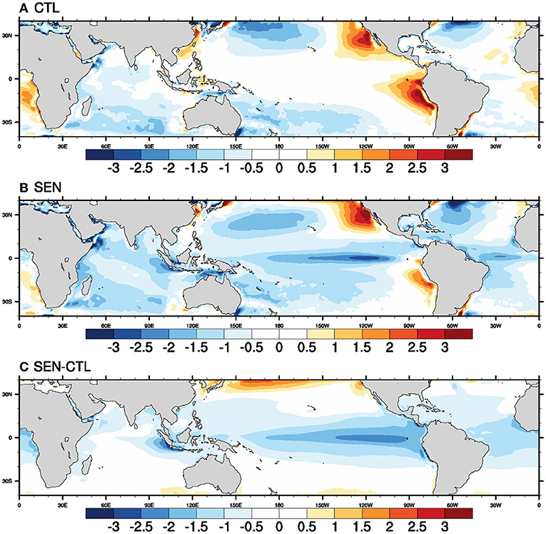
Figure 8. Seasonal (JJAS) mean bias in temperature (°C) at 5 m depth of the ocean in (A) CTL run, (B) SEN run, and (C) SEN-CTL for the period of 1981–2017.

Impact on Rainfall

Most of the general circulation models, including atmosphere standalone and ocean-atmosphere coupled models, have various problems in simulating seasonal mean rainfall patterns over the globe (Sperber et al., 2013; Goswami et al., 2014; Pillai et al., 2021; Pradhan et al., 2021; Reeves Eyre et al., 2021). Earlier studies reported that the standalone models overestimate the rainfall over the land region, whereas the coupled models underestimate (overestimate) the rainfall over landmass (ocean). Similar seasonal mean rainfall biases can be seen in both model simulations presented in Figure 9. In the CTL run, the oceanic wet bias over the northeastern and western Pacific Ocean, eastern and central Indian Ocean, and northern Atlantic Ocean are significant and have a magnitude of 4–8 mm/day. In the SEN run, the oceanic wet bias is weak as compared to the CTL run. The oceanic biases over these regions are reduced by 3–5 mm/day. Over the southwest Indian Ocean, the wet biases are enhanced by 3–4 mm/day in the SEN run. In SEN, the bias pattern in rainfall (and many of the other parameters like SW, LW) is similar to rainfall anomalies during a positive IOD event. The dry bias over central African landmass is reduced (by 2–3 mm/day), whereas it remained unaffected over South America in the SEN run compared to the CTL run. In the CTL run, the monsoon rainfall has a dry bias over the Western Ghat and, central and northern Indian landmass, and the bias is of the order of 5–7 mm/day. Interestingly, the dry bias is reduced by 2–4 mm/day over the same regions. The reduction in dry bias can be attributed to: (1) enhanced diurnal rainfall activities as discussed in section Diurnal Precipitation, (2) strengthened monsoon south-Westerlies, and (3) the modification of regional Hadley cell over the Indian Ocean region due to rainfall biases associated with positive diploe (Ashok et al., 2001) as reflected in Figure 9B.

FIGURE 9

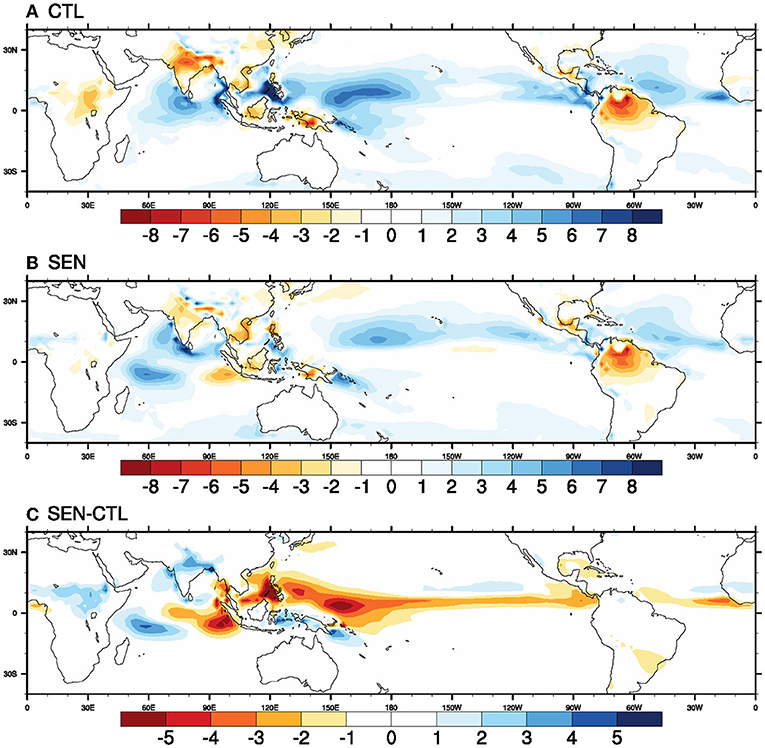
Figure 9. Seasonal (JJAS) mean bias in precipitation rate (mm/day) in (A) CTL run, (B) SEN run, and (C) SEN-CTL for the period of 1981–2017.

Impact on Global Teleconnections

The changes in the mean state of the ocean and atmospheric parameters can significantly modulate various large-scale teleconnection, impacting prediction skills. To achieve better seasonal prediction, it is crucial to properly simulate global scale teleconnection patterns and the appropriate representation of the mean state (Pillai et al., 2018). The correlation between ISMR and SST anomalies represents the ISMR-SST teleconnection over the global oceans. During the study period in observation/reanalysis, the negative impact of El Niño events on ISMR can be seen from (Figure 10) negative correlations over the eastern and central Pacific oceans. Over the Indian Ocean, the negative correlations over the eastern Indian Ocean suggest that cooler SSTs over the eastern Indian Ocean favor more rainfall over Indian landmass, similar to the impact of positive dipole events (Saji et al., 1999; Ashok et al., 2001). The ISMR-SST relation over the Indian Ocean is not as strong as the correlations over the Pacific Ocean. However weaker negative correlations over the western Indian Ocean are observed in recent times, unlike the positive correlations reported in earlier studies (Pradhan et al., 2017) for a different study period (1976–2005). In most climate models, the ENSO-monsoon relation is reasonably well-simulated with some over-estimation of the ENSO impact on monsoons (Chattopadhyay et al., 2016; Li et al., 2017; Pradhan et al., 2017, 2021). However, the present-day climate models still have inherent problems in simulating realistic IOD-ISMR correlations (Wu et al., 2007; Li et al., 2017; Pradhan et al., 2017). In both the model runs, the adverse impact of El Niño events on ISMR is well-simulated. The negative correlations over the equatorial Pacific Ocean in CTL run are vastly overestimated.

FIGURE 10

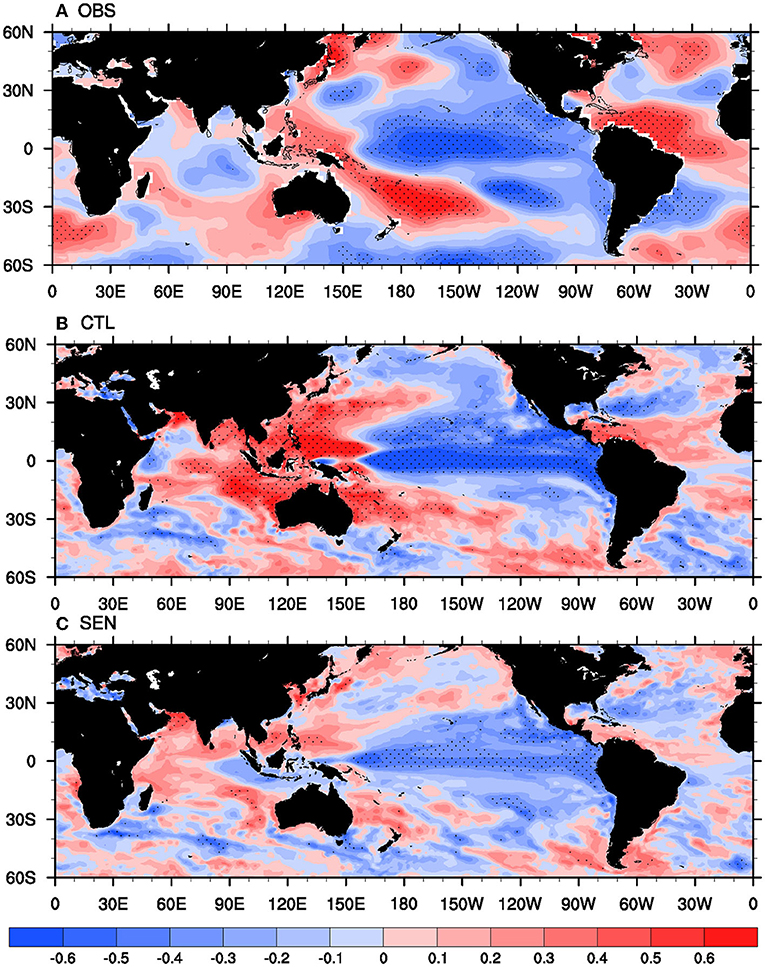
Figure 10. Correlation coefficient between ISMR and seasonal mean SST for the period 1981–2017 in (A) observation, (B) CTL, and (C) SEN run. The black dots show regions where correlation is significant at 90% confidence level.

Interestingly, the overestimation is significantly subdued in the SEN run but keeps correlations' negative sign intact. Hence, ENSO-monsoon teleconnections are modulated considerably in SEN run as compared to the CTL run. Over the Indian Ocean, in the CTL run simulation, the correlation pattern is just opposite to the observation, with strong negative correlations prevailing on the western side and positive correlations prevailing on the eastern side of the Indian Ocean. Li et al. (2017) have reported that most climate models have similar problems where positive IOD is associated with reducing rainfall over India. Wu et al. (2007) have reported an improper relationship between surface heat fluxes (specifically with latent heat) and SST over the eastern Indian Ocean in CFSv2 due to overestimating heat fluxes. In the SEN run, the teleconnections have improved over the eastern Indian Ocean as it simulates weak negative correlations over the same region. The reduction in heat flux biases resulting from revised flux and skin temperature parameterization has modulated the teleconnection patterns so that the correct phase of ISMR-SST teleconnections could be simulated over the eastern Indian Ocean as well. Hence, the association of IOD events with ISMR is better reproduced in the SEN run than in the CTL run.

Impact on ENSO and IOD Characteristics

The improved diurnal and seasonal mean state and variability of atmospheric and oceanic parameters and their teleconnections with implementing the COARE3.0 bulk flux algorithm motivated us to look at the changes in ENSO and IOD characteristics over the tropical Pacific and the Indian Ocean. In Figure 11, skewness of de-trended SST anomalies is plotted for reanalysis and both the model simulations. Skewness is the third moment about mean and describes the asymmetry about the mean of the probability distribution function of a random variable. The skewness of SSTs can be positive, negative, or zero, with a positive (negative) value describing a stronger probability of extremes in warmer (cooler) SSTs, and zero value means the distribution function is not skewed in any direction. In observation/reanalysis, positive skewness over the eastern and central tropical Pacific Ocean and negative skewness over the western Pacific Ocean suggest that the El-Niño events are stronger than the La-Niña events. In the CTL run, difficulty in simulating the skewness values of SST can be seen. Negative values throughout the equatorial Pacific do not agree with observation and show the limitation of the CTL run in capturing the ENSO-related non-linearity. Most of the models have similar difficulty capturing the non-linearity associated with the ENSO (Masson et al., 2012). SEN runs still have a similar difficulty in simulating the positive skewness in SST over the eastern Pacific. However, the SEN run simulates positive skewness values between 180 and 120°W, and negative skewness values are organized in horse-shoe patterns around the positive skewness values. Hence, the ENSO-related non-linearity is simulated better in the SEN run than the CTL run. Similar inferences are drawn by Masson et al. (2012). They have reported that with high-frequency ocean-atmosphere coupling, the non-linearity associated with ENSO phenomena (i.e., positive skewness over the central and eastern equatorial Pacific and negative skewness over the western Pacific Ocean) are better reproduced in the Scale Interaction Experiment-Frontier (SINTEX) model. They have further stated that the erroneous negative skewness similar to the CTL simulation affects ENSO variability at seasons, including peak El Niño events.

FIGURE 11

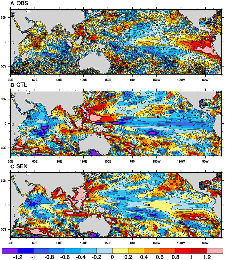
Figure 11. Skewness of de-trended SST anomaly during JJAS in (A) observation, (B) CTL run, and (C) SEN run for the period of 1981–2017.

On the other hand, the negative skewness along 150–100°W adversely affects only springtime ENSO variabilities instead of the peak ENSO phase. In the observation, negative skewness over the eastern Indian Ocean and positive skewness over the western and central Indian Ocean suggest that positive IOD events are stronger than negative ones. Contrary to observation, the CTL run has strong positive (negative) skewness over the eastern (western) Indian Ocean. However, the SEN run reproduced the negative skewness as in observation lacking in the CTL run. Also, the SEN run shows that the negative skewness has decreased in magnitude over the central and western Indian oceans. Therefore, intra-daily skin temperature parameterization present in the COARE algorithm helps better simulate the non-linearity associated with both ENSO and IOD phenomena which were significantly lacking with the default flux algorithm in the CTL run.

Impact on Seasonal Prediction Skill

Due to model inherent biases and the philosophy behind seasonal prediction, the operational forecasts focus on predicting the anomaly patterns and the variability instead of the absolute value of various parameters. SST signals are slowly varying boundary conditions that have higher predictability than the fast-varying atmospheric parameter. Therefore, monitoring and forecasting SST anomalies with good skill are essential for predicting other parameters and keeping in mind the large-scale impacts they carry. The effect of revised surface flux parameterization on diurnal and seasonal mean state and variability and interannual teleconnections has been discussed earlier. The discussion on the modeling effort cannot be complete without assessing its impact on the seasonal forecast skill. The seasonal prediction skill of a forecasting model for a particular parameter is commonly assessed via anomaly correlation coefficient (ACC) between the observation/reanalysis and predicted/re-forecasted values. Figures 12A,B shows the skill of SST (5 m ocean temperature to be precise) in terms of ACC for both the simulations. At a lead of 3 months, the SST skill is higher than 0.4 over most global oceans. Higher skill over the Pacific Ocean compared to other basins is seen because of the higher predictability of ENSO signals (Rowell et al., 1995; Goswami, 1998; Rowell, 1998). Over the Indian Ocean, the eastern and western Indian Ocean, Arabian Sea, and BoB have higher skills than the central Indian Ocean. The comparison of ACC in both the simulations suggests significant improvement of skill over the whole tropical Pacific. In the CTL run, the ACC magnitude ranges from 0.4 to 0.6 in most tropical Pacific with some patches where ACC ranges from 0.6 to 0.8. In the SEN run, throughout the tropical Pacific, the ACC magnitude lies between 0.6 and 0.8. Over the Indian Ocean, ACC of SST remains similar, with a slight enhancement in skill over the central equatorial Indian Ocean. Over the northern Atlantic, the spatial extension of significant ACC is enhanced. Therefore, the inclusion of the COARE3.0 flux algorithm and the cool skin and warm layer correction significantly impact SST prediction skills.

FIGURE 12

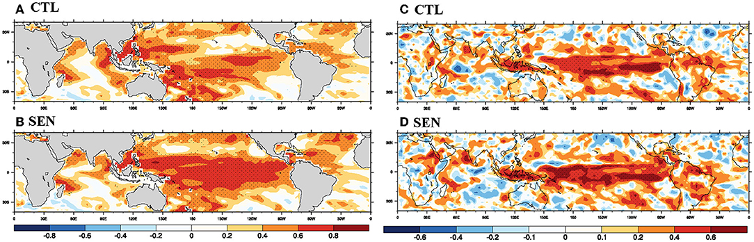
Figure 12. Prediction skill in terms of anomaly correlation coefficient (ACC) for SST during JJAS in (A) CTL run, (B) SEN run for the period of 1981–2017. (C,D) same as (A,B), but for precipitation.

Similarly, the prediction skill for rainfall anomalies is also compared for the model simulations in Figures 12C,D. As mentioned earlier, due to the higher predictability of ENSO signals, the tropical Pacific has higher anomaly correlations than other ocean basins and landmasses. Higher ACC, over the equatorial Pacific, specifically at the western and central equatorial Pacific, can be seen in the SEN run compared to the CTL run. Similarly, enhanced prediction skill of rainfall along the monsoon south-westerlies and the Arabian Sea and reduced skill over the eastern Indian Ocean can be seen. Over central Africa and eastern parts of South American landmass, the magnitude of ACC of rainfall is increased. The prediction skill of monsoon rainfall is also significantly affected, and higher ACC can be seen in the Western Ghats and northern Indian landmass. As discussed earlier, the regions with enhanced prediction skills over Africa and Indian landmass coincide with areas with reduced dry bias. In our previous studies, Pillai et al. (2018, 2021), Krishna et al. (2019), and Pradhan et al. (2021), it was found that the global models with cooler SST bias predict a higher mean value of monsoon rainfall. Still, the prediction skill of SST and rainfall anomalies are less in those models.

Interestingly, in the present study, despite cooler SST bias, both the dry bias and prediction skill of rainfall are enhanced along with higher prediction skill of SST anomalies. The prediction skill of various climate monitoring indices is presented in Table 3, suggesting the enhanced prediction skill of NIÑO3.4, NIÑO3, and ISMR, whereas the prediction skill of the DMI index remains unaffected. The improvement in the mean of ISMR in the SEN run compared to the CTL run is computed to be 38% (5.52 mm/day in SEN run from 4.01 mm/day in CTL run), whereas the prediction skill is improved by 38% (0.40 in SEN run from 0.29 in CTL run).

TABLE 3

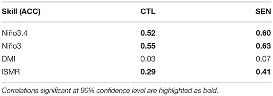
Table 3. Prediction skill represented in terms of anomaly correlation coefficient for ISMR and SST indices for the period 1981–2017.

Summary and Discussion

Literature comprises many observational studies regarding accurate air-sea boundary conditions leading to the development of various bulk flux algorithms. Precise representation of air-sea boundary through accurate quantification of surface fluxes and sea surface temperature can reduce the biases in global coupled models. The studies regarding the choice of bulk flux algorithms are limited to either one-dimensional or standalone ocean (or atmosphere) models. The COARE 3.0 is one of the most frequently used bulk flux algorithms used to generate turbulent flux products from observed surface meteorological and oceanic parameters. However, the use of COARE3.0 in the coupling framework in seasonal prediction models has not been tested or addressed elaborately, citing its higher computational resource requirement in coupled models. This study shows the feasibility of the COARE3.0 algorithm in a seasonal prediction framework using the CFSv2 model. The study also addressed how the diurnal to seasonal scale coupled model simulations with COARE3.0 and NCAR algorithms differ. The default version of CFSv2 with NCAR and the modified version with COARE3.0 algorithm differ because the former model does not account for the diurnal warm layer and cool skin corrections in the ocean skin temperature, whereas the latter does. Also, they differ in the parameterization of stability functions and roughness lengths and hence also differ in the quantification of surface fluxes. The diurnal analysis indicated that, in the absence of diurnal scale parameterization, diurnal mixing of the upper ocean is not represented well in the CTL run, leading to underestimating the diurnal range of MLD and SST compared to observation. Also, the timing of maxima/minima of MLD and or SST is incorrect in the CTL run at a few locations over the Indian and Pacific Oceans.

On the other hand, implementing the skin temperature scheme in the SEN run as part of the COARE3.0 algorithm results in an amplified diurnal range of SST and MLD compared to the CTL run and improvement in the timing of diurnal maxima/minima of SST and MLD. The modification of diurnal SST, MLD, and turbulent fluxes in the SEN run has also impacted the spatiotemporal characteristics of diurnal precipitation. The diurnal rainfall range is amplified over the tropical Indo-Pacific Ocean in the SEN run, which was hugely underestimated in default CFSv2 compared to observation. As reported in earlier observational studies, the amplification of in diurnal range in rainfall manifests a rise in diurnal SST, which acts as a trigger for shallow cloud convection. Analysis of seasonal mean from both simulations suggests that the mean biases in surface fluxes, MLD, and precipitation have reduced with COARE3.0 compared to default CFSv2. The reduced dry bias over the land regions, specifically over Indian landmass, is due to the enhanced diurnal range in precipitation and the enhanced seasonal mean monsoon south-westerlies in the SEN run. However, the seasonal mean SST bias (5 m ocean temperature) increased with the COARE algorithm compared to with the NCAR algorithm. The decrease in seasonal mean SST with diurnal corrections is due to higher cool-skin events than warm-layer events because the prevailing winds are stronger during June-September. The present study also addressed how sensitive the ENSO, IOD characteristics, and various Indo-Pacific teleconnections patterns are to the choice of bulk flux algorithm and diurnal scale temperature parameterization. Implementing the COARE3.0 algorithm has improved simulation of non-linearity (presented in terms of skewness of SST) and linear association of SST-rainfall (presented in terms of anomaly correlation) during ENSO and IOD events. The positively skewed SST over the central equatorial Pacific and negatively skewed SST over the eastern Indian Ocean is well-represented in CFSv2 with COARE 3.0 and were missing in the default CFSv2 simulations. The ISMR-SST teleconnection over the Indo-Pacific basin has improved significantly in the SEN run because of the improved ocean-atmosphere coupling. The overestimation of ENSO-monsoon teleconnection and negative dipole like ISMR-SST correlations over the Indian Ocean are long-existing problems in many global models, including CFSv2. These teleconnection patterns are significantly improved and corrected in CFSv2 with COARE3.0 by revising the surface flux algorithm along with diurnal skin temperature corrections. The improvement in dry bias in ISMR (5.52 mm/day in SEN run from 4.01 mm/day in the CTL run) is around 38%. The prediction skill (ACC) of the Niño3.4 (Niño3) index is significantly improved from 0.52 (0.55) in default CFSv2 to 0.60 (0.63) in CFSv2 with COARE3.0. ISMR prediction skill for the study period is also reported to improve by 38% (from 0.29 to 0.40) by revising the bulk flux algorithm.

Therefore, the present study documents how the inclusion flux parameterization of COARE 3.0 improved the diurnal SST representation in the coupled model, and resulted in significant improvements of the diurnal to the seasonal mean state of ocean-atmosphere parameters, ENSO-IOD characteristics, Indo-Pacific teleconnections, and seasonal prediction skill of ISMR and SST indices. Although the present study briefly discussed the implications of selecting diurnal skin temperature and flux parameterization in a coupled model, it does not discuss its impact at an intraseasonal scale, i.e., at a scale intermediate between diurnal and seasonal scales. Hence it sets the future scope of addressing how coupled processes such as the monsoon intra-seasonal oscillation (MISO), Madden-Jullian Oscillation (MJO), etc., are sensitive to the choice of bulk flux algorithm in coupled models.

Data Availability Statement

The raw data supporting the conclusions of this article will be made available by the authors, without undue reservation.

Author Contributions

The analysis, plotting, and preparation of the manuscript were done by MP. SR, AB, and SB contributed by formulating the problem and writing and editing the final manuscript. All authors contributed to the article and approved the submitted version.

Funding

Indian Institute of Tropical Meteorology was fully funded by Ministry of Earth Sciences, Government of India.

Conflict of Interest

The authors declare that the research was conducted in the absence of any commercial or financial relationships that could be construed as a potential conflict of interest.

Publisher's Note

All claims expressed in this article are solely those of the authors and do not necessarily represent those of their affiliated organizations, or those of the publisher, the editors and the reviewers. Any product that may be evaluated in this article, or claim that may be made by its manufacturer, is not guaranteed or endorsed by the publisher.

Supplementary Material

The Supplementary Material for this article can be found online at: https://www.frontiersin.org/articles/10.3389/fclim.2021.792980/full#supplementary-material

References

Adler, R. F., Sapiano, M., Huffman, G. J., Wang, J., Gu, G., Bolvin, D., et al. (2018). The Global Precipitation Climatology Project (GPCP) monthly analysis (new version 2.3) and a review of 2017 global precipitation. Atmosphere 9:40138. doi: 10.3390/atmos9040138

PubMed Abstract | CrossRef Full Text

Ashok, K., Guan, Z., and Yamagata, T. (2001). Impact of the Indian Ocean dipole on the relationship between the Indian monsoon rainfall and ENSO. Geophys. Res. Lett. 28, 4499–4502. doi: 10.1029/2001GL013294

PubMed Abstract | CrossRef Full Text | Google Scholar

Beljaars, A. C. M., and Holtslag, A. A. M. (1991). Flux parameterization over land surfaces for atmospheric models. J. Appl. Meteorol. Climatol. 30, 327–341. doi: 10.1175/1520-0450(1991)030<0327:FPOLSF>2.0.CO;2

CrossRef Full Text | Google Scholar

Bellenger, H., and Duvel, J.-P. (2009). An analysis of tropical ocean diurnal warm layers. J. Climate 22, 3629–3646. doi: 10.1175/2008JCLI2598.1

CrossRef Full Text | Google Scholar

Bellenger, H., Takayabu, Y. N., Ushiyama, T., and Yoneyama, K. (2010). Role of diurnal warm layers in the diurnal cycle of convection over the tropical Indian Ocean during MISMO. Monthly Weather Rev. 138, 2426–2433. doi: 10.1175/2010MWR3249.1

CrossRef Full Text | Google Scholar

Bernie, D. J., Guilyardi, E., Madec, G., Slingo, J. M., and Woolnough, S. J. (2007). Impact of resolving the diurnal cycle in an ocean–atmosphere, G. C. M. Part 1: a diurnally forced OGCM. Climate Dyn. 29, 575–590. doi: 10.1007/s00382-007-0249-6

CrossRef Full Text | Google Scholar

Bernie, D. J., Guilyardi, E., Madec, G., Slingo, J. M., Woolnough, S. J., and Cole, J. (2008). Impact of resolving the diurnal cycle in an ocean–atmosphere, G. C. M. Part 2: a diurnally coupled CGCM. Climate Dyn. 909–925. doi: 10.1007/s00382-008-0429-z

CrossRef Full Text | Google Scholar

Blanc, T. V. (1987). Accuracy of bulk-method-determined flux, stability, and sea surface roughness. J. Geophys. Res. 92:3867. doi: 10.1029/JC092iC04p03867

CrossRef Full Text | Google Scholar

Bonino, G., Iovino, D., and Masina, S. (2020). TN0289 - Bulk Formulations in NEMOv.4: Algorithms Review and Sea Surface Temperature Response in ORCA025 Case Study - CMCC. Centro Euro-Mediterraneo sui Cambiamenti Climatici, Lecce, Italy, 1–25.

Google Scholar

Brunke, M. A., Zeng, X., and Anderson, S. (2002). Uncertainties in sea surface turbulent flux algorithms and data sets. J. Geophys. Res. 107:992. doi: 10.1029/2001JC000992

CrossRef Full Text | Google Scholar

Brunke, M. A., Zeng, X., Misra, V., and Beljaars, A. (2008). Integration of a prognostic sea surface skin temperature scheme into weather and climate models. J. Geophys. Res. Atmos. 113:D21117. doi: 10.1029/2008JD010607

CrossRef Full Text | Google Scholar

Chang, H.-R., and Grossman, R. L. (1999). Evaluation of bulk surface flux algorithms for light wind conditions using data from the coupled ocean-atmosphere response experiment (COARE). Quart. J. Royal Meteorol. Soc. 125, 1551–1588. doi: 10.1002/qj.49712555705

PubMed Abstract | CrossRef Full Text | Google Scholar

Chattopadhyay, R., Rao, S. A., Sabeerali, C. T., George, G., Rao, D. N., Dhakate, A., et al. (2016). Large-scale teleconnection patterns of Indian summer monsoon as revealed by CFSv2 retrospective seasonal forecast runs. Int. J. Climatol. 36, 3297–3313. doi: 10.1002/joc.4556

PubMed Abstract | CrossRef Full Text | Google Scholar

Chen, S. S., and Houze, R. A. (1997). Diurnal variation and life-cycle of deep convective systems over the tropical pacific warm pool. Quart. J. Royal Meteorol. Soc. 123, 357–388. doi: 10.1002/qj.49712353806

PubMed Abstract | CrossRef Full Text | Google Scholar

Clayson, C. A., and Chen, A. (2002). Sensitivity of a coupled single-column model in the tropics to treatment of the interfacial parameterizations. J. Climate 15, 1805–1831. doi: 10.1175/1520-0442(2002)015<1805:SOACSC>2.0.CO;2

CrossRef Full Text | Google Scholar

Curry, J. A., Bentamy, A., Bourassa, M. A., Bourras, D., Bradley, E. F., Brunke, M., et al. (2004). SEAFLUX. Bullet. Am. Meteorol. Soc. 85, 409–424. doi: 10.1175/BAMS-85-3-409

CrossRef Full Text | Google Scholar

Dai, A., and Trenberth, K. E. (2004). The diurnal cycle and its depiction in the community climate system model. J. Climate. 17, 930–951. doi: 10.1175/1520-0442(2004)017<0930:TDCAID>2.0.CO;2

CrossRef Full Text | Google Scholar

Dyer, A. J. (1974). A review of flux-profile relationships. Bound. Layer Meteorol. 7, 363–372. doi: 10.1007/BF00240838

CrossRef Full Text | Google Scholar

Edson, J. B., Jampana, V., Weller, R. A., Bigorre, S. P., Plueddemann, A. J., Fairall, C. W., et al. (2013). On the exchange of momentum over the open ocean. J. Phys. Oceanogr. 43, 1589–1610. doi: 10.1175/JPO-D-12-0173.1

CrossRef Full Text | Google Scholar

Ek, M. B., Mitchell, K. E., Lin, Y., Rogers, E., Grunmann, P., Koren, V., et al. (2003). Implementation of Noah land surface model advances in the National Centers for Environmental Prediction operational mesoscale Eta model. J. Geophys. Res. 108, 8851. doi: 10.1029/2002JD003296

CrossRef Full Text | Google Scholar

Fairall, C. W., Bradley, E. F., Godfrey, J. S., Wick, G. A., Edson, J. B., and Young, G. S. (1996a). Cool-skin and warm-layer effects on sea surface temperature. J. Geophys. Res. 101, 1295–1308. doi: 10.1029/95JC03190

CrossRef Full Text | Google Scholar

Fairall, C. W., Bradley, E. F., Hare, J. E., Grachev, A. A., and Edson, J. B. (2003). Bulk parameterization of air-sea fluxes: updates and verification for the COARE algorithm. J. Climate 16, 571–591. doi: 10.1175/1520-0442(2003)016<0571:BPOASF>2.0.CO;2

CrossRef Full Text | Google Scholar

Fairall, C. W., Bradley, E. F., Rogers, D. P., Edson, J. B., and Young, G. S. (1996b). Bulk parameterization of air-sea fluxes for tropical ocean-global atmosphere coupled-ocean atmosphere response experiment. J. Geophys. Res. 101:3747. doi: 10.1029/95JC03205

CrossRef Full Text | Google Scholar

Ganai, M., Krishna, R. P. M., Mukhopadhyay, P., and Mahakur, M. (2016). The impact of revised simplified Arakawa-Schubert scheme on the simulation of mean and diurnal variability associated with active and break phases of Indian summer monsoon using CFSv2. J. Geophys. Res. 121, 9301–9323. doi: 10.1002/2016JD025393

PubMed Abstract | CrossRef Full Text | Google Scholar

George, G., Rao, D. N., Sabeerali, C. T., Srivastava, A., and Rao, S. A. (2016). Indian summer monsoon prediction and simulation in CFSv2 coupled model. Atmos. Sci. Lett. 17, 57–64. doi: 10.1002/asl.599

PubMed Abstract | CrossRef Full Text | Google Scholar

Goswami, B. B., Deshpande, M., Mukhopadhyay, P., Saha, S. K., Rao, S. A., Murthugudde, R., et al. (2014). Simulation of monsoon intraseasonal variability in NCEP CFSv2 and its role on systematic bias. Climate Dyn. 43, 2725–2745. doi: 10.1007/s00382-014-2089-5

CrossRef Full Text | Google Scholar

Goswami, B. N. (1998). Interannual variations of Indian summer monsoon in a GCM: external conditions versus internal feedbacks. J. Climate 11, 501–522. doi: 10.1175/1520-0442(1998)011<0501:IVOISM>2.0.CO;2

CrossRef Full Text | Google Scholar

Griffies, S. M., Harrison, M. J., Pacanowski, R. C., and Rosati, A. (2004). A Technical Guide to MOM4, GFDL Ocean Group Technical Report No. 5. NOAA/Geophysical Fluid Dynamics Laboratory. Available online at: www.gfdl.noaa.gov. (accessed August 23, 2004).

Google Scholar

Huang, B., Thorne, P. W., Banzon, V. F., Boyer, T., Chepurin, G., Lawrimore, J. H., et al. (2017). Extended reconstructed sea surface temperature, version 5 (ERSSTv5): upgrades, validations, and intercomparisons. J. Climate 30, 8179–8205. doi: 10.1175/JCLI-D-16-0836.1

CrossRef Full Text | Google Scholar

Huffman, G. J., Adler, R. F., Bolvin, D. T., and Nelkin, E. J. (2010). The TRMM multi-satellite precipitation analysis (TMPA). Satellite Rainfall Appl. Surf. Hydrol. 1, 3–22. doi: 10.1007/978-90-481-2915-7_1

CrossRef Full Text | Google Scholar

Johnson, R. H., Rickenbach, T. M., Rutledge, S. A., Ciesielski, P. E., and Schubert, W. H. (1999). Trimodal characteristics of tropical convection. J. Climate 12, 2397–2418. doi: 10.1175/1520-0442(1999)012<2397:TCOTC>2.0.CO;2

CrossRef Full Text | Google Scholar

Kawai, Y., and Wada, A. (2007). Diurnal sea surface temperature variation and its impact on the atmosphere and ocean: a review. J. Oceanogr. 63, 721–744. doi: 10.1007/s,10872-007-0063-0

CrossRef Full Text | Google Scholar

KBRR, H. P., Pentakota, S., Anguluri, S. R., George, G., Salunke, K., Krishna, P. M., et al. (2020). Impact of horizontal resolution on sea surface temperature bias and air–sea interactions over the tropical Indian Ocean in CFSv2 coupled model. Int. J. Climatol. 40, 4903–4921. doi: 10.1002/joc.6496

PubMed Abstract | CrossRef Full Text | Google Scholar

Kim, H., Lee, M. I., Cha, D. H., Lim, Y. K., and Putman, W. M. (2019). Improved representation of the diurnal variation of warm season precipitation by an atmospheric general circulation model at a 10 km horizontal resolution. Climate Dyn. 53, 6523–6542. doi: 10.1007/s00382-019-04943-6

CrossRef Full Text | Google Scholar

Krishna, R. P. M., Rao, S. A., Srivastava, A., Kottu, H. P., Pradhan, M., Pillai, P., et al. (2019). Impact of convective parameterization on the seasonal prediction skill of Indian summer monsoon. Climate Dyn. 53, 6227–6243. doi: 10.1007/s00382-019-04921-y

CrossRef Full Text | Google Scholar

Krishnamurti, T. N., and Bhalme, H. N. (1976). Oscillations of a monsoon system. Part, I. Observational aspects. J. Atmos. Sci. 33, 1937–1954. doi: 10.1175/1520-0469(1976)033<1937:OOAMSP>2.0.CO;2

CrossRef Full Text | Google Scholar

Kumar, B. P., Vialard, J., Lengaigne, M., Murty, V. S. N., and McPhaden, M. J. (2012). TropFlux: air-sea fluxes for the global tropical oceans-description and evaluation. Climate Dyn. 38, 1521–1543. doi: 10.1007/s00382-011-1115-0

CrossRef Full Text | Google Scholar

Large, W. G., and Yeager, S. G. (2004). Diurnal to Decadal Global Forcing for Ocean and Sea–Ice Models: {The} Data Sets and Flux Climatologies. NCAR Tech. Note, TN–460+ST(May), Colorado, National Center for Atmospheric Research Boulder, 105.

Google Scholar

Large, W. G., and Yeager, S. G. (2008). The global climatology of an interannually varying air–sea flux data set. Climate Dyn. 33, 341–364. doi: 10.1007/s00382-008-0441-3

CrossRef Full Text | Google Scholar

Li, W., Yu, R., Liu, H., and Yu, Y. (2001). Impacts of diurnal cycle of SST on the intraseasonal variation of surface heat flux over the western pacific warm pool. Adv. Atmos. Sci. 18, 793–806. doi: 10.1007/BF03403503

CrossRef Full Text | Google Scholar

Li, Z., Lin, X., and Cai, W. (2017). Realism of modelled Indian summer monsoon correlation with the tropical Indo-Pacific affects projected monsoon changes. Sci. Rep. 7, 1–7. doi: 10.1038/s41598-017-05225-z

PubMed Abstract | CrossRef Full Text | Google Scholar

Madden, R. A., and Julian, P. R. (1971). Detection of a 40–50 day oscillation in the zonal wind in the tropical pacific. J. Atmos. Sci. 28, 702–708. doi: 10.1175/1520-0469(1971)028<0702:DOADOI>2.0.CO;2

CrossRef Full Text | Google Scholar

Madden, R. A., and Julian, P. R. (1972). Description of global-scale circulation cells in the tropics with a 40-50 day period. - NASA/ADS. J. Atmos. Sci. 29, 1109–1123. doi: 10.1175/1520-0469(1972)029<1109:DOGSCC>2.0.CO;2

CrossRef Full Text | Google Scholar

Mallick, S. K., Agarwal, N., Sharma, R., Prasad, K. V. S. R., and Ramakrishna, S. S. V. S. (2020). Thermodynamic response of a high-resolution tropical indian ocean model to toga coare bulk air-sea flux parameterization: case study for the bay of bengal (BoB). Pure Appl. Geophys. 177, 4025–4044. doi: 10.1007/S00024-020-02448-6/FIGURES/11

CrossRef Full Text | Google Scholar

Mao, J. Y., and Wu, G. X. (2012). Diurnal variations of summer precipitation over the Asian monsoon region as revealed by TRMM satellite data. Sci. China Earth Sci. 55, 554–566. doi: 10.1007/s11430-011-4315-x

CrossRef Full Text | Google Scholar

Masson, S., Terray, P., Madec, G., Luo, J. J., Yamagata, T., and Takahashi, K. (2012). Impact of intra-daily SST variability on ENSO characteristics in a coupled model. Climate Dyn. 39, 681–707. doi: 10.1007/s00382-011-1247-2

CrossRef Full Text | Google Scholar

Misra, V., Marx, L., Brunke, M., and Zeng, X. (2008). The equatorial pacific cold tongue bias in a coupled climate model. J. Climate 21, 5852–5869. doi: 10.1175/2008JCLI2205.1

CrossRef Full Text | Google Scholar

Montégut, C. de. B., Madec, G., Fischer, A. S., Lazar, A., and Iudicone, D. (2004). Mixed layer depth over the global ocean: an examination of profile data and a profile-based climatology. J. Geophys. Res. 109, 1–20. doi: 10.1029/2004JC002378

CrossRef Full Text | Google Scholar

Moorthi, S., Pan, H-L., and Caplan, P. (2001). Changes to the 2001 NCEP Operational MRF/AVN Global Analysis/Forecast System Technical Procedures Bulletin Changes to the 2001 NCEP Operational MRF/AVN Global Analysis/Forecast System. National Weather Service, Office of Meteorology, Technical Procedures Bulletin, Silver Spring, MD, United States.

Mujumdar, M., Salunke, K., Rao, S. A., Ravichandran, M., and Goswami, B. N. (2011). Diurnal cycle induced amplification of sea surface temperature intraseasonal oscillations over the bay of Bengal in summer monsoon season. IEEE Geosci. Remote Sens. Lett. 8, 206–210. doi: 10.1109/LGRS.2010.2060183

PubMed Abstract | CrossRef Full Text | Google Scholar

Neelin, J. D., Battisti, D. S., Hirst, A. C., Jin, F.-F., Wakata, Y., Yamagata, T., et al. (1998). ENSO theory. J. Geophys. Res. 103:14261. doi: 10.1029/97JC03424

CrossRef Full Text | Google Scholar

Philander, S. G. H. (1985). El Niño and La Niña. J. Atmos. Sci. 42, 2652–2662. doi: 10.1175/1520-0469(1985)042<2652:ENALN>2.0.CO;2

CrossRef Full Text | Google Scholar

Pillai, P. A., Rao, S. A., George, G., Rao, D. N., Mahapatra, S., Rajeevan, M., et al. (2017). How distinct are the two flavors of El Niño in retrospective forecasts of Climate Forecast System version 2 (CFSv2)? Climate Dyn. 48, 3829–3854. doi: 10.1007/s00382-016-3305-2

CrossRef Full Text | Google Scholar

Pillai, P. A., Rao, S. A., Ramu, D. A., Pradhan, M., and George, G. (2018). Seasonal prediction skill of Indian summer monsoon rainfall in NMME models and monsoon mission CFSv2. Int. J. Climatol. 38, e847–e861. doi: 10.1002/joc.5413

PubMed Abstract | CrossRef Full Text | Google Scholar

Pillai, P. A., Rao, S. A., Srivastava, A., Ramu, D. A., Pradhan, M., and Das, R. S. (2021). Impact of the tropical Pacific SST biases on the simulation and prediction of Indian summer monsoon rainfall in CFSv2, ECMWF-System4, and NMME models. Climate Dyn. 56, 1699–1715. doi: 10.1007/s00382-020-05555-1

CrossRef Full Text | Google Scholar

Pokhrel, S., Rahaman, H., Parekh, A., Saha, S. K., Dhakate, A., Chaudhari, H. S., et al. (2012). Evaporation-precipitation variability over Indian Ocean and its assessment in NCEP Climate Forecast System (CFSv2). Climate Dyn. 39, 2585–2608. doi: 10.1007/s00382-012-1542-6

CrossRef Full Text | Google Scholar

Pradhan, M., Rao, S. A., Doi, T., Pillai, P. A., Srivastava, A., and Behera, S. (2021). Comparison of MMCFS and SINTEX-F2 for seasonal prediction of Indian summer monsoon rainfall. Int. J. Climatol. 41, 6084–6108. doi: 10.1002/joc.7169

PubMed Abstract | CrossRef Full Text | Google Scholar

Pradhan, M., Yadav, R. K., Ramu Dandi, A., Srivastava, A., Phani, M. K., and Rao, S. A. (2017). Shift in MONSOON–SST teleconnections in the tropical Indian Ocean and ENSEMBLES climate models' fidelity in its simulation. Int. J. Climatol. 37, 2280–2294. doi: 10.1002/joc.4841

PubMed Abstract | CrossRef Full Text | Google Scholar

Ramu, D. A., Sabeerali, C. T., Chattopadhyay, R., Rao, D. N., George, G., Dhakate, A. R., et al. (2016). Indian summer monsoon rainfall simulation and prediction skill in the CFSv2 coupled model: impact of atmospheric horizontal resolution. J. Geophys. Res. 121, 2205–2221. doi: 10.1002/2015JD024629

PubMed Abstract | CrossRef Full Text | Google Scholar

Rao, S. A., Behera, S. K., Masumoto, Y., and Yamagata, T. (2002). Interannual subsurface variability in the tropical Indian Ocean with a special emphasis on the Indian Ocean Dipole. Deep Sea Res. II Top. Stud. Oceanogr. 49, 1549–1572. doi: 10.1016/S0967-0645(01)00158-8

CrossRef Full Text | Google Scholar

Rao, S. A., Goswami, B. N., Sahai, A. K., Rajagopal, E. N., Mukhopadhyay, P., Rajeevan, M., et al. (2019). Monsoon Mission: a targeted activity to improve monsoon prediction across scales. Bullet. Am. Meteorol. Soc. 100, 2509–2532. doi: 10.1175/BAMS-D-17-0330.1

CrossRef Full Text | Google Scholar

Reeves Eyre, J. E. J., Zeng, X., and Zhang, K. (2021). Ocean surface flux algorithm effects on earth system model energy and water cycles. Front. Mar. Sci. 403:642804. doi: 10.3389/fmars.2021.642804

CrossRef Full Text | Google Scholar

Rowell, D. P. (1998). Assessing potential seasonal predictability with an ensemble of multidecadal GCM simulations. J. Climate. 11, 109–120. doi: 10.1175/1520-0442(1998)011<0109:APSPWA>2.0.CO;2

CrossRef Full Text | Google Scholar

Rowell, D. P., Folland, C. K., Maskell, K., and Ward, M. N. (1995). Variability of summer rainfall over tropical north Africa (1906–92): observations and modelling. Quart. J. Royal Meteorol. Soc. 121, 669–704. doi: 10.1256/smsqj.52310

CrossRef Full Text | Google Scholar

Saha, S., Moorthi, S., Pan, H., Wu, X., Wang, J., Nadiga, S., et al. (2010). NCEP Climate Forecast System Reanalysis (CFSR) 6-hourly Products, January 1979 to December 2010. Research Data Archive at the National Center for Atmospheric Research, Computational and Information Systems Laboratory. doi: 10.5065/D69K487J

CrossRef Full Text | Google Scholar

Saha, S., Moorthi, S., Wu, X., Wang, J., Nadiga, S., Tripp, P., et al. (2014). The NCEP climate forecast system version 2. J. Clim. 27, 2185–2208. doi: 10.1175/JCLI-D-12-00823.1

CrossRef Full Text | Google Scholar

Saji, N. H., Goswami, B. N., Vinayachandran, P. N., and Yamagata, T. (1999). A dipole mode in the tropical Indian Ocean. Nature 401, 360–363. doi: 10.1038/43854

PubMed Abstract | CrossRef Full Text | Google Scholar

Shinoda, T. (2005). Impact of the diurnal cycle of solar radiation on intraseasonal SST variability in the western equatorial pacific. J. Climate 18, 2628–2636. doi: 10.1175/JCLI3432.1

CrossRef Full Text | Google Scholar

Slingo, J., Inness, P., Neale, R., Woolnough, S., and Yang, G. (2003). Scale interactions on diurnal toseasonal timescales and their relevanceto model systematic errors. Ann. Geophys. 46:3383. doi: 10.4401/ag-3383

CrossRef Full Text | Google Scholar

Smith, S. D. (1988). Coefficients for sea surface wind stress, heat flux, and wind profiles as a function of wind speed and temperature. J. Geophys. Res. 93, 15467–15472. doi: 10.1029/JC093iC12p15467

CrossRef Full Text | Google Scholar

Sperber, K. R., Annamalai, H., Kang, I. S., Kitoh, A., Moise, A., Turner, A., et al. (2013). The Asian summer monsoon: An intercomparison of CMIP5 vs. CMIP3 simulations of the late 20th century. Climate Dynamics. 41, 2711–2744. doi: 10.1007/s00382-012-1607-6

CrossRef Full Text | Google Scholar

Stuart-Menteth, A. C., Robinson, I. S., and Challenor, P. G. (2003). A global study of diurnal warming using satellite-derived sea surface temperature. J. Geophys. Res. 108:3155. doi: 10.1029/2002JC001534

CrossRef Full Text | Google Scholar

Sui, C.-H., Takayabu, Y. N., and Short, D. A. (1997). Diurnal variations in tropical oceanic cumulus convection during TOGA COARE. J. Atmos. Sci. 54, 639–655. doi: 10.1175/1520-0469(1997)054<0639:DVITOC>2.0.CO;2

CrossRef Full Text | Google Scholar

Thushara, V., and Vinayachandran, P. N. (2014). Impact of diurnal forcing on intraseasonal sea surface temperature oscillations in the Bay of Bengal. J. Geophys. Res. Oceans. 119, 8221–8241. doi: 10.1002/2013JC009746

PubMed Abstract | CrossRef Full Text | Google Scholar

Weare, B. C. (1989). Uncertainties in estimates of surface heat fluxes derived from marine reports over the tropical and subtropical oceans. Tellus A 41A, 357–370. doi: 10.1111/j.1600-0870.1989.tb00388.x

CrossRef Full Text | Google Scholar

Winton, M. (2000). A reformulated three-layer sea ice model. J. Atmos. Ocean. Technol. 17, 525–531. doi: 10.1175/1520-0426

CrossRef Full Text | Google Scholar

Woolnough, S. J., Vitart, F., and Balmaseda, M. A. (2007). The role of the ocean in the Madden-Julian Oscillation: implications for MJO prediction. Quart. J. Royal Meteorol. Soc. 133, 117–128. doi: 10.1002/qj.4

CrossRef Full Text | Google Scholar

Wu, R., Kirtman, B. P., and Pegion, K. (2007). Surface latent heat flux and its relationship with sea surface temperature in the National Centers for Environmental Prediction Climate Forecast System simulations and retrospective forecasts. Geophys. Res. Lett. 34, 2–7. doi: 10.1029/2007GL030751

CrossRef Full Text | Google Scholar

Yan, Y., Zhang, L., Yu, Y., Chen, C., Xi, J., and Chai, F. (2021). Rectification of the intraseasonal SST variability by the diurnal cycle of SST revealed by the global tropical moored buoy array. Geophys. Res. Lett. 48:e2020GL090913. doi: 10.1029/2020GL090913

CrossRef Full Text | Google Scholar

Yang, G-Y., and Slingo, J. (2001). The diurnal cycle in the tropics. monthly weather review. Bull. Am. Meteorol. Soc. 129, 784–801. doi: 10.1175/1520-0493(2001)129

CrossRef Full Text | Google Scholar

Yasunari, T. (1980). A quasi-stationary appearance of 30 to 40 day period in the cloudiness fluctuations during the summer monsoon over India. J. Meteorol. Soc. Jap. Ser. II Meteorol. Soc. Jap. 58, 225–229. doi: 10.2151/jmsj1965.58.3_225

PubMed Abstract | CrossRef Full Text | Google Scholar

Yu, L., Jin, X., and Weller, R. (2008). Multidecade Global Flux Datasets from the Objectively Analyzed Air-sea Fluxes (OAFlux) Project: Latent and Sensible Heat Fluxes, Ocean Evaporation, and Related Surface Meteorological Variables. OAFlux Project Technical Report, Falmouth, Massachusetts, Woods Hole Oceanographic Institution, OA-2008-01( 74).

Google Scholar

Zeng, X., Zhao, M., and Dickinson, R. E. (1998). Intercomparison of bulk aerodynamic algorithms for the computation of sea surface fluxes using TOGA COARE and TAO data. J. Climate 11, 2628–2644. doi: 10.1175/1520-0442(1998)011<2628:IOBAAF>2.0.CO;2

CrossRef Full Text | Google Scholar

Zhang, R., Wang, X., and Wang, C. (2018). On the simulations of global oceanic latent heat flux in the CMIP5 multimodel ensemble. J. Climate 31, 7111–7128. doi: 10.1175/JCLI-D-17-0713.1

CrossRef Full Text | Google Scholar

Zhang, R., Zhou, F., Wang, X., Wang, D., and Gulev, S. K. (2020). Cool Skin Effect and its Impact on the Computation of the Latent Heat Flux in the South China Sea. J. Geophy. Res. Oceans. 126, 2020JC016498. doi: 10.1029/2020JC016498

CrossRef Full Text | Google Scholar

Zheng, Y., Shinoda, T., Lin, J.-L., and Kiladis, G. N. (2011). Sea surface temperature biases under the stratus cloud deck in the southeast pacific ocean in 19 IPCC AR4 coupled general circulation models. J. Climate 24, 4139–4164. doi: 10.1175/2011JCLI4172.1

CrossRef Full Text | Google Scholar

Zhou, X., Ray, P., Barrett, B. S., and Hsu, P.-C. (2020). Understanding the bias in surface latent and sensible heat fluxes in contemporary AGCMs over tropical oceans. Climate Dyn. 55, 2957–2978. doi: 10.1007/s00382-020-05431-y

CrossRef Full Text | Google Scholar