Decadal variability of the interannual climate predictability associated with the Indo-Pacific oceanic channel dynamics in CCSM4

Introduction

The Pacific and Indian Oceans span over two-thirds of the global longitudinal domain. The variability of the ocean in this part of the earth is of great importance to global climate variability and predictability. The strong interannual modes of climate variability in the Pacific and the Indian Oceans, the El Niño-Southern Oscillation (ENSO) and the Indian Ocean Dipole (IOD), interact with each other through the Walker Circulation (Klein et al., 1999; Alexander et al., 2002; Clarke and Gorder, 2003; Lau and Nath, 2003; Lau et al., 2005; Kug et al., 2006; Luo et al., 2010). This process is called the atmospheric bridge.

The two oceans are also connected by the Indonesian Throughflow (ITF). The precursory relation between IOD and ENSO is suggested recently by Yuan et al. (2011, 2013), indicating that the upwelling anomalies in the southeastern tropical Indian Ocean (STIO) during a positive IOD event propagate through the Indonesian seas and elevate the thermocline of the western Pacific warm pool. The anomalies then propagate to the eastern Pacific cold tongue to induce significant sea surface temperature anomalies (SSTA) and climate variations at the time lag of 1 year. This process is named the “oceanic channel” dynamics by Yuan et al. (2011), in contrast to the atmospheric bridge process.

Enhanced predictability of ENSO at the lead time of 1 year across the spring persistence barrier has been suggested if anomalies over the tropical Indian Ocean are used as a predictor (Clarke and Gorder, 2003; Izumo et al., 2010; Luo et al., 2010; Zhou et al., 2015). Analyses have suggested that about half of the cold tongue SSTA standard deviation can be predicted at the one-year lead when IOD anomalies are used as precursors. Lag correlation analyses have suggested that the oceanic channel dynamics are important for the interannual predictability of the tropical Indo-Pacific climate across the spring barrier (Yuan et al., 2011, 2013, 2017; Xu et al., 2013), the equatorial wave dynamics of which have been investigated by Yuan et al. (2018). The oceanic channel dynamics are evidenced by the propagation of sea level from the STIO to the western equatorial Pacific Ocean, giving rise to the significant lag correlations between the oceanic anomalies in STIO in fall and those in the Pacific equatorial vertical section and in the cold tongue at the one-year time lag (Yuan et al., 2013). Recent studies have also suggested that the IOD-ENSO teleconnection is subject to decadal and multi-decadal variations (Xu et al., 2013; Izumo et al., 2014; Xu and Yuan, 2015), the dynamics of which are not clear at present.

The decadal variability of the IOD-ENSO precursory teleconnection has been shown to have positive and negative phases alternatively by Xu and Yuan (2015), using the long time series of the Simple Ocean Data Assimilation (SODA) data. The results have shown that the oceanic channel dynamics prevail during both the positive and negative phases of the decadal variability. Deeper thermocline in the eastern equatorial Pacific was identified during the negative phases of the decadal variability than during the positive phases, which explains the disappearing or even reversing of the IOD-ENSO precursory relation.

The SODA data are a forced ocean assimilation not dynamically consistent in general. In this study, the experiments of the Community Climate System Model version 4 (CCSM4) that participates in the Coupled Model Intercomparison Project phase-5 (CMIP5) are used to evaluate the skills of the model in simulating the IOD-ENSO precursory relation during the positive phases of the decadal variability. The dynamics of the inter-basin precursory relation are investigated and the skills of the models in simulating the precursory relation through the oceanic channel and the atmospheric bridge are assessed.

The paper is organized as the following. Section Data and model introduces the observational data and the model simulations used in the study. Section Results presents the results of the lag correlation analyses of the CCSM4 model simulations during the positive phases of the decadal variability, which are compared with the analyses based on observational data. Comparisons of the oceanic channel dynamics during the positive and negative phases of the decadal variability and the effects of the anthropogenic forcing are discussed in Section Discussions. Conclusions are summarized in Section Conclusions of this paper.

Data and model

Gridded observational data

The observed sea surface temperature (SST) data used in this study are the Hadley Center sea Ice and SST data (HadISST) covering the global ocean from 1870 to near present with a resolution of 1° longitude by 1° latitude (Rayner et al., 2003), the extended reconstruction of global SST (ERSST V3b) covering the global ocean from 1854 to present on a 2° × 2° horizontal grid (Smith et al., 2008), and the Kaplan SST (Version 2.0) covering the global ocean from 1856 to present on a 5° × 5°grid (Kaplan et al., 1998). The sea surface height data are the merged altimeter data from the Aviso project on a global grid of 1/3° longitude by 1/3° latitude resolution from 1993 to present. The subsurface temperature data are on a grid of 5° longitude by 2° latitude at 11 levels from 1990 to 2003, which are obtained from the Joint Environmental Data Analysis Center of the Scripps Institution of Oceanography (White, 1995). The National Center for Environmental Prediction/National Center for Atmospheric Research (NCEP/NCAR) reanalysis surface wind data are on a 2.5° × 2.5° grid from 1948 to present (Kalnay et al., 1996).

Observations of the ITF transport

The only long-term measurement of the ITF transport in existence to date is the geostrophic transport based on the XBT data along the IX1 section between the western Australia and the Java island since 1987. The geostrophic transport is in reference to the 700 m level-of-no-motion, with a statistical temperature-salinity relation based on historical hydrographic data employed in the calculation (Meyers et al., 1995; Meyers, 1996; Wijffels and Meyers, 2004; Wijffels et al., 2008; Yuan et al., 2013). Interannual monthly anomalies of the ITF transport are calculated based on the monthly climatology from 1987 to 2008.

The CCSM4 model experiments

The model used in this study is the fourth version of the Community Climate System Model (CCSM4; Gent et al., 2011), which is composed of four geophysical models simulating the earth's atmosphere (the Community Atmosphere Model version 5; Neale et al., 2013), ocean (the Parallel Ocean Program version 2; Smith et al., 2010), land surface (the Community Land Model version 4; Lawrence et al., 2011), and sea-ice (the Los Alamos Sea Ice Model; Hunke and Lipscomb, 2008). The communications among the four component models are coordinated by a coupler (CPL7; Craig et al., 2012). The ocean component of CCSM4 uses a grid with a varying latitudinal resolution, increasing from 0.54° poleward of 33° N and 33°S to 0.27° near the equator, a uniform 1.125° longitudinal resolution, and 60 irregular vertical levels. A horizontal grid of zonal 1.25° by meridional 0.9° is used in the atmospheric component of CCSM4, which contains 26 layers in the vertical direction. CCSM4 is found to have a few improvements in the periodicity, range, amplitude, and duration simulations of ENSO and IOD events, compared to its predecessor CCSM3 (Gent et al., 2011; Deser et al., 2012).

The long-term “historical” and “historicalNat” simulations of CCSM4 of the CMIP5 project are used in this study (Taylor et al., 2012). In the CMIP5 project, the performance of the coupled models of the international communities is compared following a standard experimental protocol (Meehl and Bony, 2011). A set of model simulations are promoted to evaluate the skills of the coupled models in simulating the recent past and projecting the climate change in the near and long future. All of the six ensemble member historical experiments are forced with both the anthropogenic and natural radiative conditions, and all of the four ensemble member historicalNat experiments are forced only with the natural forcing, which are used to conduct the analyses in this study. Both the historical and historicalNat experiments were initialized randomly (Taylor et al., 2012) and have covered the industrial period from the mid-19th century to the present.

Statistical analysis

In this study, several used indices are as follows. The Niño3.4 index is calculated as the area-averaged SSTA in the equatorial central-eastern Pacific Ocean (5°S-5°N, 170°W-120°W). The Dipole Mode Index (DMI) is defined as the difference of area-averaged SSTA between the southeastern (10°S-equator, 90°E-110°E) and the western (10°S-10°N, 50°E-70°E) tropical Indian Ocean areas (Saji et al., 1999).

Throughout the paper, the lag correlation is calculated between the area-averaged oceanic anomalies in STIO (10°S-equator, 90°E-110°E) or the surface zonal wind anomalies (SZWA) in fall over the far western equatorial Pacific (5°S-5°N, 130°E-150°E) in boreal fall and the anomalies over the Indo-Pacific Oceans in the following four seasons. Boreal seasons, defined as winter (the last December to February), spring (March to May), summer (June to August), and fall (September to November), are used throughout this paper. We will call the IOD year Year 0 and the year following it Year +1. The composite lag correlation analyses are applied in the study, while the time series during positive or negative phases are concatenated after normalized, respectively. In the CCSM4 simulations, the positive or negative phases are determined in each individual ensemble member before concatenated together. The partial correlation analyses are used in removing the ENSO signals. The confidence levels of the correlations and the spectra are computed based on the Student's-t test and the red noise test, respectively.

Results

In this section, the decadal variability of the IOD-ENSO precursory relation at the one-year time lead is first analyzed based on the SST observations. The simulated decadal variability in the CCSM4 experiments is then evaluated in comparison with the observational analysis, based on which the dynamics and predictability of the IOD-ENSO teleconnection during the positive and negative decadal phases and their modification by the anthropogenic forcing are investigated.

Decadal variability of the IOD-ENSO teleconnection

The positive IOD peaks in fall with significant upwelling anomalies generated in STIO, which propagate into the Indonesian seas in the form of coastal Kelvin waves. The lag correlations between the SSTA in STIO in fall and the Niño3.4 SSTA at the one-year time lag have been calculated in running windows of 7, 9, and 11 years, showing consistent decadal variations in the three observational SST datasets, i.e., HadISST, ERSST, and Kaplan SST (Figure 1). The 7, 9, and 11-year running lag correlations are consistent with each other, with the 11-year running correlations basically the smoothed variability of the 7 and 9-year running correlations. The differences of the running lag correlations among the three SST datasets are larger before than after the 1950's, probably due to the low quality of the SSTA observations before WWII. All of the three SST datasets indicate that the IOD-ENSO lag correlation is strongly positive during the latest decades since the 1990's, consistent with the analysis of Yuan et al. (2013). In this study, the time series during 1946–1965 and 1992–2009, two of the latest positive phases of the decadal variability (periods of the positive running lag correlations), are normalized and concatenated to conduct the lag correlation calculation. Due to the short running windows, the lag correlations in Figure 1 generally do not pass the 95% confidence test. However, the lag correlations between the STIO SSTA in fall and the Niño3.4 SSTA at the one-year lag based on the normalized and concatenated time series are statistically significant (see Subsection Lag correlations of SSTA). In addition, the spectra have shown that the running correlations have decadal oscillations above the 95% confidence level at 10–20 years.

FIGURE 1

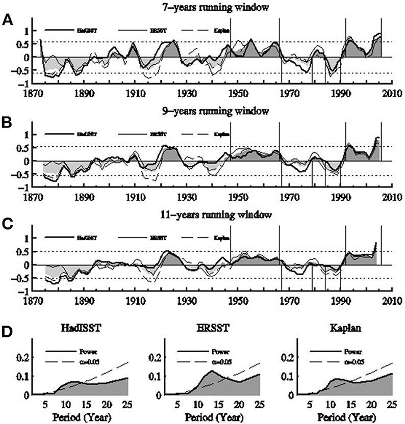
Figure 1. Decadal variability of the IOD-ENSO correlation at the one-year time lag in HadISST, ERSST, and Kaplan SST data. The lag correlations between the SSTA in STIO in fall and the Niño3.4 SSTA in the following fall are calculated in 7-year (A), 9-year (B), and 11-year (C) sliding windows, with the vertical axis showing window central year. Horizontal dashed lines indicate 95% confidence level. The bottom panel (D) shows the power spectra of the lag correlations in the 7-year sliding window with statistics calculated from 1945 to 2009. Dash curves indicate 95% confidence level based on the Student's-t test. Vertical lines mark the positive and negative phase periods.

The running lag correlations are negative during some of the decades, suggesting that El Niños sometimes followed positive IODs and La Niñas followed negative IODs at the one-year time lag. Thus, the IOD-ENSO relations during the negative phases of the decadal variability are different from those during the positive phases. The running lag correlations have shown that the negative phases of the decadal variability are weaker and of short duration than the positive phases over the past 150 years or so, with coefficients of skewness of 11-year running correlations are−0.19 for HadISST,−0.15 for ERSST and−0.23 for Kaplan SST respectively. The means and standard deviations of the 7-year running correlations are all consistently larger during the two positive phases than during the two latest negative phases of 1968–1979 and 1984–1989 for all three SST datasets (Table 1). There is also a trend that the negative lag correlations are getting weaker and of shorter duration while the positive lag correlations are getting stronger and of longer duration over the latest decades. The linear trends of the 7-year running lag correlations are 0.0040 per year, 0.0032 per year, and 0.0044 per year for the HadISST, ERSST, and Kaplan SST datasets, respectively. For these reasons, we will focus on the IOD-ENSO teleconnection during the positive phases of the decadal variability in this paper.

TABLE 1

Table 1. Comparison of the means and standard deviations of the 7-year running lag correlations during the positive and negative phases based on the three SST datasets.

Model validation

All of the six ensemble member experiments of the CCSM4 historical simulation exhibit decadal variability of the IOD-ENSO precursory relation, as evidenced by the decadal variability of the lag correlations calculated in the 7–11 year running windows between the simulated STIO SSTA in fall and the Niño3.4 SSTA at the one-year lag (Figure 2). The amplitudes and phases of the decadal variability in each ensemble experiments are different due to different initial conditions of the simulations. The spectra of the running lag correlations in all six ensemble experiments clearly indicate the existence of the decadal variability at periods of 10–20 years. The agreement of the simulated and the observed periods of the decadal variability suggests that the CCSM4 simulations can be used to investigate the dynamics of the decadal IOD-ENSO teleconnection variability.

FIGURE 2

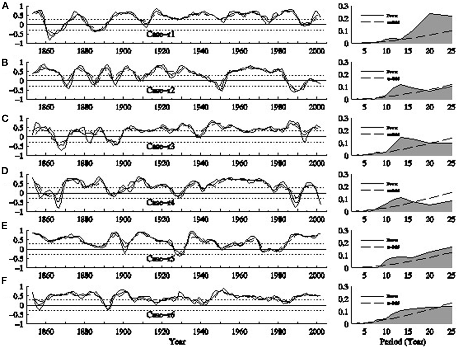
Figure 2. Decadal variability of the IOD-ENSO lag correlations in CCSM4 simulations (all six ensemble experiments). The lag correlations between the SSTA in STIO in fall and the Niño3.4 indices in the following fall are calculated in all six historical ensemble cases (A–F) in 7-year (solid curve), 9-year (dash curve), and 11-year (dash dot curve) sliding windows. Horizontal dashed lines indicate the positive and negative phases (positive lag correlations above the upper dashed line and negative phased under the lower dashed line). The right column shows the power spectra of the lag correlations in the 7 years sliding window with statistics calculated based on all the six ensemble experiments. Dash curves indicate 95% confidence level based on the Student's-t test.

The regression coefficients between DMI with SSTA in the Indian Ocean and those between Niño3.4 index with SSTA in the Pacific Ocean show zonal dipole patterns in the two basins (Figure 3). The similar dipole patterns in the simulation and in the observations suggest that the IOD and ENSO spatial patterns are simulated well by the CCSM4 coupled system. The model is also able to simulate the periodicity of ENSO well. The simulated periodicity of IOD is slightly longer than the observed, probably due to stronger dominance of ENSO in the model simulations.

FIGURE 3

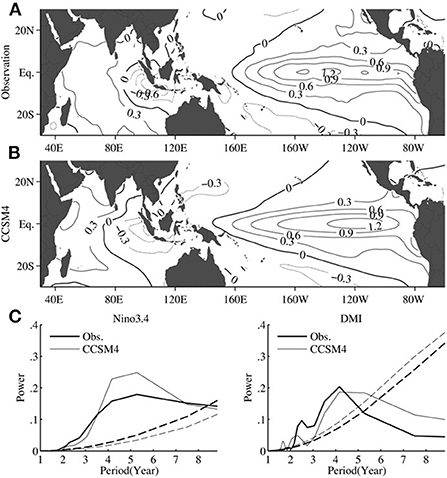
Figure 3. Comparison of the observed [(A); HadISST] and simulated (B) regression coefficients between the DMI index and the SSTA in the Indian Ocean and between the Niño3.4 index and the SSTA in the Pacific Ocean. The simulated regression coefficients are calculated based on the simulated DMI and Niño3.4 index. Bottom panels (C) show the power spectra of the observed and simulated Niño3.4 and DMI indices, respectively. Dash curves indicate 95% confidence level based on the red noise test.

Lag correlations of SSTA

The six ensemble members of the CCSM4 historical simulation have been analyzed and their correlations are calculated based on the normalized and concatenated time series during the positive phases of the decadal variability for each of the ensemble experiments. All six ensemble members share nearly the same lag correlation patterns between the SSTA (SSHA) in STIO in fall and the tropical Indo-Pacific SSTA (SSHA) in the following four seasons during different phases of the decadal variability. Therefore, only the lag correlations based on the normalized and concatenated SSTA time series of all of the six ensemble CCSM4 historical simulations are presented for analysis.

The lag correlations between the STIO SSTA in fall and the Indo-Pacific SSTA in the following winter through fall seasons based on the concatenated SSTA time series during the positive phases of the decadal variability in the HadISST data and in the six ensemble CCSM4 historical simulations are compared in Figure 4. The observational analyses are based on the HadISST anomalies during positive phases of the decadal variability since 1945. The significant lag correlations in winter both in the observations and in the model show negative correlations in the eastern Pacific, but positive correlations in the western Pacific and eastern Indian Oceans, consistent with the IOD and ENSO dipole patterns (Figure 4A). These patterns can be explained by the fact that IOD frequently occur in synchrony with ENSO.

FIGURE 4

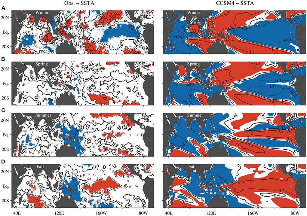
Figure 4. Comparison of observed (left column) and simulated (right column) lag correlations between the SSTA in STIO in fall and the tropical Indo-Pacific SSTA in the following four seasons during the positive phases of the decadal variability (from 1945 to 2009 in the observation). (A) Winter (December to February). (B) Spring (March to May). (C) Summer (June to August). (D) Autumn (September to November). The contour interval is 0.3. Red and blue shades indicate 95% confidence level of positive and negative correlation, respectively. The model correlations are nearly everywhere above the 95% significance level due to the long time series.

The lag correlations in the observations and in the model in the equatorial zone fall both decrease in spring, consistent with the existence of the spring barrier. Significant lag correlations, exceeding the 95% confidence level, but with an opposite sign to those in winter, appear in the central equatorial Pacific in the observations and in the central-to-eastern equatorial Pacific cold tongue in the model in the fall of Year +1, which suggest that some ENSO events can be predicted effectively at the one-year time lead if IOD is used as a precursor during the positive decadal phases.

It is noticed that the lag correlations in the cold tongue in the fall of Year +1 in the model are stronger and over a larger longitudinal domain than in the observations (Figure 4D). The reason of the difference will be discussed in detail later in Subsection Effects of the atmospheric bridge, which is due to unrealistic wind simulations in the model during the decay phase of the ENSO and IOD events.

Because of the long distance and the potential low penetration rate of the Kelvin wave signals from the Indian Ocean through the Indonesian seas, the effects of the IOD on the cold tongue SSTA are believed to be amplified by the coupled ocean and atmosphere interaction over the tropical Pacific Ocean (Yuan et al., 2011). Therefore, the majority of the ENSO signals are produced by the coupled amplification over the tropical Pacific Ocean. If we should remove the ENSO signal associated with the Niño3.4 index from the SSTA, which is essentially equivalent to the removal of the coupling effects, the lag correlations between the STIO SSTA in fall and the cold tongue non-ENSO SSTA at the one-year time lag are still significant (figure omitted, see Yuan et al., 2013). The analyses suggest that the IOD-cold tongue SSTA teleconnection at the one-year time lag during the positive phases of the decadal variability is robust.

Lag correlations of SSHA

The lag correlations between the STIO sea surface height anomalies (SSHA) in fall and the Indo-Pacific SSHA in the following winter through fall seasons based on the normalized and concatenated time series during the positive phases of the decadal variability in all of the six ensemble CCSM historical simulations are calculated in Figure 5. The area-averaged SSHA in STIO in fall are used to represent the IOD Kelvin waves. The lag correlations of the observed SSHA are calculated based on the satellite altimeter data since 1993. The lag correlations of the CCSM4 simulations on the equator are in good agreement with those based on satellite altimeter data. The SSHA lag correlations in the winter of Year 0 show the IOD and ENSO dipole patterns similar to the SSTA lag correlations, with the lag correlations in the western Indian Ocean and the eastern Pacific cold tongue in opposite signs with those in the eastern Indian Ocean and the western Pacific (Figure 5A). The lag correlations in spring through summer suggest eastward propagation of correlated SSHA from the STIO to the western equatorial Pacific through the Indonesian seas both in the model and in the observations (Figure 5B). The propagation of the upwelling anomalies then elevate the thermocline and produce subsurface temperature anomalies in the western and central-eastern equatorial Pacific Ocean in the summer and fall of Year +1 as indicated by the movement of the significant positive correlations in Figures 5C,D. The narrow meridional bands of the propagating significant correlations suggest the influence of the equatorial Kelvin waves. The above comparisons suggest that CCSM4 is capable of simulating the essential structure of the oceanic channel dynamics in the historical experiments.

FIGURE 5

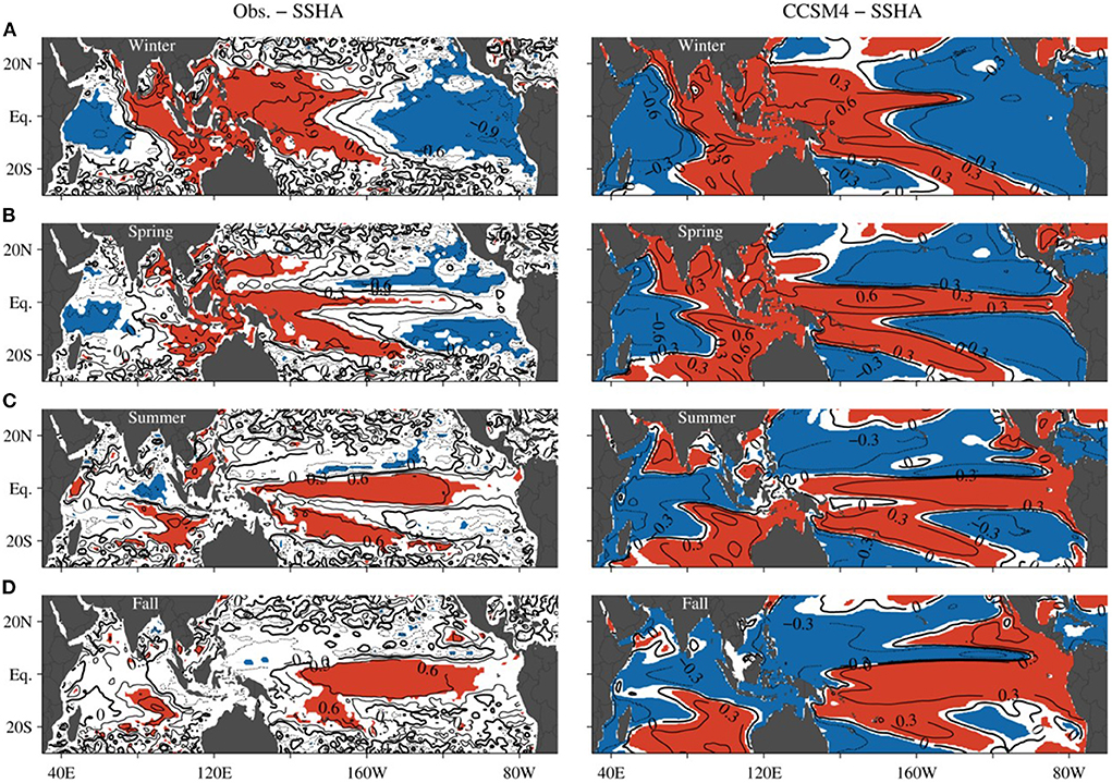
Figure 5. Comparison of observed (left column) and simulated (right column) lag correlations between the SSHA in STIO in fall and the tropical Indo-Pacific SSHA in the following four seasons during the positive phases of the decadal variability (from 1993 to 2009 in the observation). (A) Winter (December to February). (B) Spring (March to May). (C) Summer (June to August). (D) Autumn (September to November). The contour interval is 0.3. Red and blue shades indicate 95% confidence level of positive and negative correlation, respectively. The model correlations are nearly everywhere above the 95% significance level due to the long time series.

The SSHA lag correlations in the cold tongue in the fall of Year +1 are also stronger and over a larger longitudinal domain in the model than in the observations, as are the SSTA lag correlations. The reason of the difference will be explained in Subsection Effects of the atmospheric bridge, which is due to model deficiency in simulating the atmospheric bridge.

To examine the dependence of the lag correlations with ENSO, the ENSO signals associated with Niño3.4 index had been removed from the Indo-Pacific SSHA time series. The lag correlations in the equatorial band of the Pacific Ocean remain significant without the ENSO signals (figure omitted), suggesting that the oceanic channel dynamics are independent of the air-sea coupling within the tropical Pacific basin.

Subsurface lag correlations

The lag correlations between the SSTA in STIO in fall and the subsurface temperature anomalies in the equatorial Pacific vertical section in the following winter through fall based on the concatenated time series during the positive phases of the decadal variability in the six ensemble CCSM historical simulations are shown in Figure 6. The oceanic channel dynamics are suggested by the lag correlations in the subsurface equatorial Pacific Ocean, showing a dipole pattern with positive values in the western basin and negative in the east in winter (Figure 6A), which become insignificant in the surface in spring, but remain significant and propagate to the east in the subsurface (Figures 6B–D). The subsurface correlations reach the surface in the eastern Pacific cold tongue in the summer through fall of Year +1, producing the significant SSTA and SSHA lag correlations at the one-year time lag in Figures 4, 5. These subsurface lag correlations and their eastward propagation in the observations has been well reproduced by the CCSM4 simulations, except that the simulated subsurface lag correlations are much stronger than the observational results. The potential predictability of ENSO beyond the spring barrier apparently lies in the subsurface connections across the equatorial Pacific basin. The overly stronger subsurface connection in the CCSM4 simulations than in the observations are erroneous and are consistent with the simulated stronger correlations between the STIO SSTA (SSHA) in fall and the SSTA (SSHA) in the eastern Pacific cold tongue at the one-year time lag (Figures 4, 5). The reason will be explained in Subsection Effects of the atmospheric bridge.

FIGURE 6

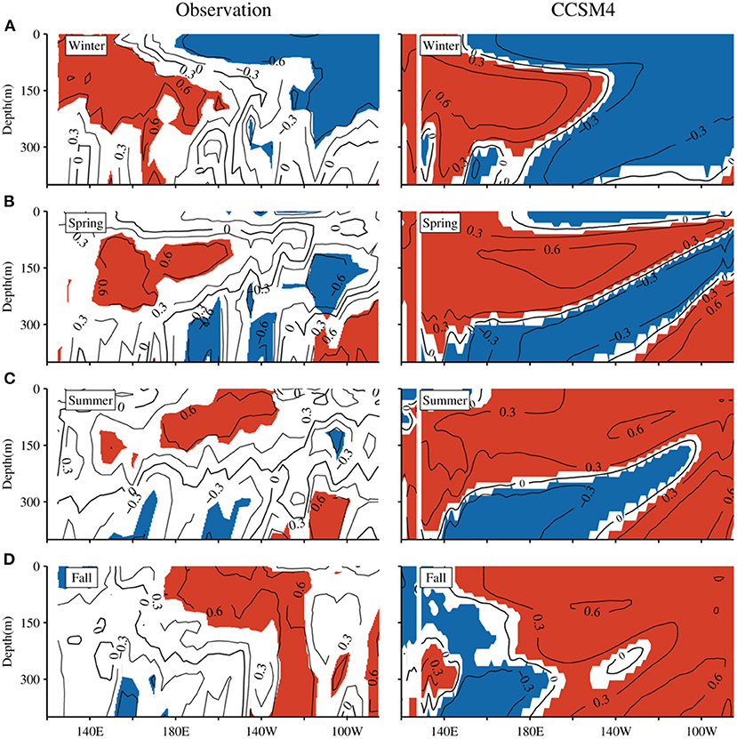
Figure 6. Comparison of observed (left column) and simulated (right column) lag correlations between the SSTA in STIO in fall and the temperature anomalies in the Pacific equatorial vertical section in the following four seasons during the positive phases of the decadal variability (from 1990 to 2003 in the observation). (A) Winter (December to February). (B) Spring (March to May). (C) Summer (June to August). (D) Autumn (September to November). The contour interval is 0.3. Red and blue shades indicate 90% confidence level of positive and negative correlation, respectively. The model correlations are nearly everywhere above the 95% significance level due to the long time series.

The lag correlations between the STIO SSTA in fall and the subsurface temperature anomalies in the Pacific vertical section with the ENSO signals removed show similar distributions of the positive correlations in the vertical section in the spring to summer of Year +1, except that the areas of the significant correlations are smaller (figure omitted). These lag correlation calculations confirm the existence of the oceanic channel dynamics and its independence from the tropical air-sea coupling both in the model and in the observations.

Variability of the ITF

The ITF volume transport and its interannual anomalies across the IX1 section are integrated by the geostrophic velocities above the main thermocline, which are calculated in reference to the 700 m level of no motion across the IX1 section from the CCSM4 simulations. The ITF transport anomalies above the main ocean thermocline have exhibited similar lag correlations with the Niño3.4 and DMI indices as the observational analyses based on the geostrophic transport above the main ocean thermocline do (Figure 7). The lag correlations between the simulated ITF transport anomalies and the simulated DMI index during the positive phases of the decadal variability are smaller than the observational analyses when ITF anomalies lead the DMI (Figures 7D,E). Similar differences also exist during the negative phases of the decadal variability. The differences suggest model deficiencies in simulating the IOD events or the ITF anomalies or both. Overall, the CCSM4 model has simulated a similar association of the ITF transport anomalies with the Niño3.4 and DMI indices, suggesting the model skills in simulating the oceanic channel dynamics between the Pacific and the Indian Oceans.

FIGURE 7

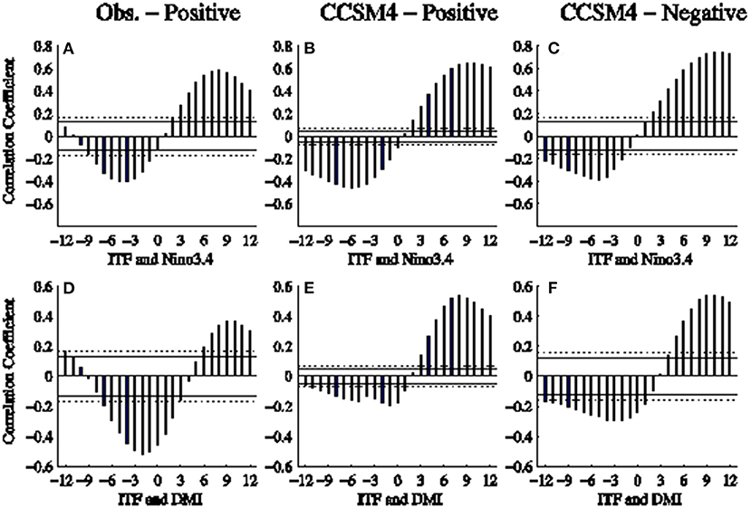
Figure 7. Lag correlations between the ITF transport anomalies and the Niño3.4 indices (A–C) or DMI (D–F) in the observations and in CCSM4 simulations. The observed (simulated) ITF transport is the geostrophic transport above the main ocean thermocline across the IX1 section between western Australia and Java in reference to the 700 m level-of-no-motion based on the XBT data (CCSM4 simulations). (A,D) are based on observational data; (B,E) are based on the CCSM4 simulations during the positive phases of the decadal variability; (C,F) are based on the CCSM4 simulations during the negative phases of the decadal variability. Solid and dashed horizontal lines represent the 95% and 99% confidence levels, respectively.

The model has simulated a mean ITF geostrophic transport of 8.7 Sv (1 Sv = 10⁶ m³ s⁻¹) from the Pacific Ocean to the Indian Ocean during the positive phases of the decadal variability, which are consistent with the observed 9.1 Sv mean geostrophic transport. The CCSM4 experiments have produced a standard deviation of the ITF interannual transports of 5.1 Sv during the positive phases of the decadal variability, in comparison with a standard deviation of 6.7 Sv in the observations. During the negative phases, the mean ITF transport and the standard deviation of its interannual anomalies are 8.8 Sv and 5.3 Sv, respectively. Evidently, the simulated interannual anomalies of the ITF geostrophic transport are significantly smaller than the observed.

The simulated weaker interannual anomalies of the ITF transport are in contrast to the stronger lag correlations in the subsurface of the equatorial Pacific vertical section in the model than in the observations (Figure 6). The stronger subsurface lag correlations are also in agreement with the stronger lag correlations between the SSTA and SSHA in STIO in fall and those in the cold tongue at the one-year time lag in the model than in the observations. This contradiction between the weaker ITF anomalies and the stronger lag correlations in the simulations than in the observations is found to be due to an overestimated atmospheric bridge in the CCSM4 climate system model, which will be discussed in the next subsection.

The simulated oceanic channel dynamics from IOD to ENSO at the one-year time lag are indicated by the lag correlations between the ITF transport anomalies in fall and the SSHA anomalies over the tropical Indo-Pacific Oceans during the positive phases of the decadal variability (Figure 8). The propagation of the Kelvin waves from STIO to the western equatorial Pacific Ocean and further to the east is indicated by the movement of the significant lag correlations. The lag correlations in Figure 8 and those of the SSHA in Figure 5 suggest strongly that the oceanic channel dynamics are at work connecting the IOD with the ENSO events at the one-year time lag.

FIGURE 8

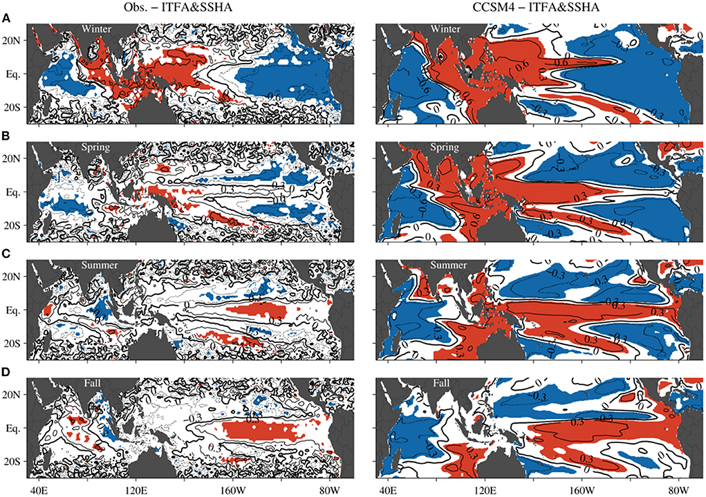
Figure 8. Comparison of observed and simulated lag correlations of ITF transport anomalies in fall with the SSHA over the Indo-Pacific Ocean in the following four seasons during the positive phases of the decadal variability. The observed (simulated) ITF transport is the geostrophic transport above the main ocean thermocline across the IX1 section between western Australia and Java in reference to the 700 m level-of-no-motion based on the XBT data (CCSM4 simulations). (A) Winter (December to February), (B) spring (March to May), (C) summer (June to August), (D) autumn (September to November). The contour interval is 0.3. Red and blue shades indicate 95% confidence level of positive and negative correlation, respectively.

Effects of the atmospheric bridge

Existing analyses of the atmospheric bridge process has had the oceanic channel dynamics incorporated by using the correlations between atmospheric anomalies and DMI, which contains the upwelling information in STIO. Yuan et al. (2013) have suggested correlating the Pacific atmospheric and ocean anomalies with the wind anomalies over the far western equatorial Pacific to examine the variations of the Walker Circulation connecting the interannual variability over the Indian and Pacific Oceans.

The lag correlations between the surface zonal wind anomalies (SZWA) averaged over the far western equatorial Pacific (5°S-5°N, 130°E-150°E) in fall with the SZWA over the Indo-Pacific oceans in the following winter through fall, based on the concatenated time series during the positive phases of the decadal variability in the observations and in the six ensemble CCSM4 historical simulations, are compared in Figure 9. The CCSM4 experiments have produced significant positive lag correlations in the eastern equatorial Pacific, and significant negative correlations in the west in the summer-fall of Year +1, which are not supported by the observational analyses at all. Evidently, CCSM4 is deficient in simulating the observed atmospheric bridge processes across the Indo-Pacific oceans. The comparisons of the lag correlations in the western-central equatorial Pacific Ocean with the observational analyses suggest that unrealistic westerly wind anomalies are produced over the equatorial Pacific in the CCSM4 simulations in Year +1, which generate downwelling equatorial Kelvin waves propagating eastward and upwelling equatorial Rossby waves propagating westward. This wind patch produces the stronger subsurface lag correlations in the model than in the observation in Figure 6 and the stronger lag correlations in the cold tongue at the one-year time lag in Figures 4, 5. The weaker ITF anomalies are evidently overwhelmed by the unrealistic wind patch so that artificially stronger subsurface anomalies in the equatorial vertical section of the Pacific Ocean in CCSM4 are generated.

FIGURE 9

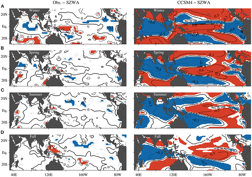
Figure 9. Comparison of observed (left column) and simulated (right column) lag correlations between the SZWA over the far western equatorial Pacific in fall and the tropical Indo-Pacific SZWA in the following four seasons during the positive phases of the decadal variability (from 1948 to 2009 in the observation). (A) Winter (December to February). (B) Spring (March to May). (C) Summer (June to August). (D) Autumn (September to November). The contour interval is 0.3. Red and blue shades indicate 95% confidence level of positive and negative correlation, respectively.

Due to the overestimated atmospheric bridge, the lag correlations between the SZWA over the far western equatorial Pacific in fall and the cold tongue SSTA in the spring through fall of Year +1 are all much stronger than in the observations (Figure 10). So are the lag correlations between the SZWA over the far western Pacific in fall and the SSHA in the cold tongue at the one-year time lag (figure omitted). The comparisons confirm the model deficiency in simulating the atmospheric bridge processes in the observations.

FIGURE 10

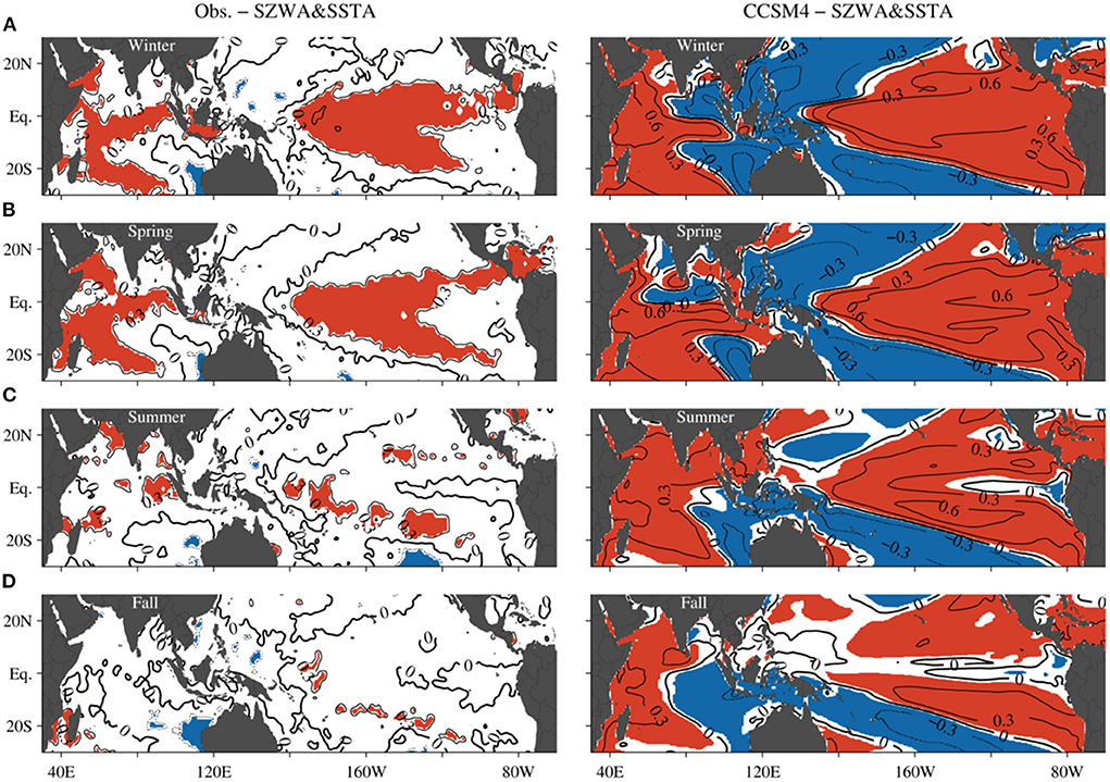
Figure 10. Comparison of observed (left column) and simulated (right column) lag correlations between the SZWA over the far western equatorial Pacific in fall and the tropical Indo-Pacific SSTA in the following four seasons during the positive phases of the decadal variability (from 1948 to 2009 in the observation). (A) Winter (December to February). (B) Spring (March to May). (C) Summer (June to August). (D) Autumn (September to November). The contour interval is 0.3. Red and blue shades indicate 95% confidence level of positive and negative correlation, respectively.

Discussions

The lag correlations of all six historical simulations of CCSM4 during the negative phases of the decadal variability have been compared with those during the positive phases. The lag correlations between the SSTA in STIO in fall and the tropical Indo-Pacific SSTA in the following winter show nearly the same teleconnection patterns during the positive and negative phases of the decadal variability, with significant positive correlations in the western Pacific and eastern Indian Oceans and significant negative correlations in the equatorial Pacific cold tongue and in the western Indian Ocean (Figure 11). The comparison suggests that the ENSO-IOD relations at near-zero time lags are the same during either phase of the decadal variability. The lag correlations during the ensuing spring through fall, however, are significantly different. In particular, the significant lag correlations in the cold tongue in the fall of Year +1 in the positive phases of the decadal variability become negative or vanishingly small in the negative phases.

FIGURE 11

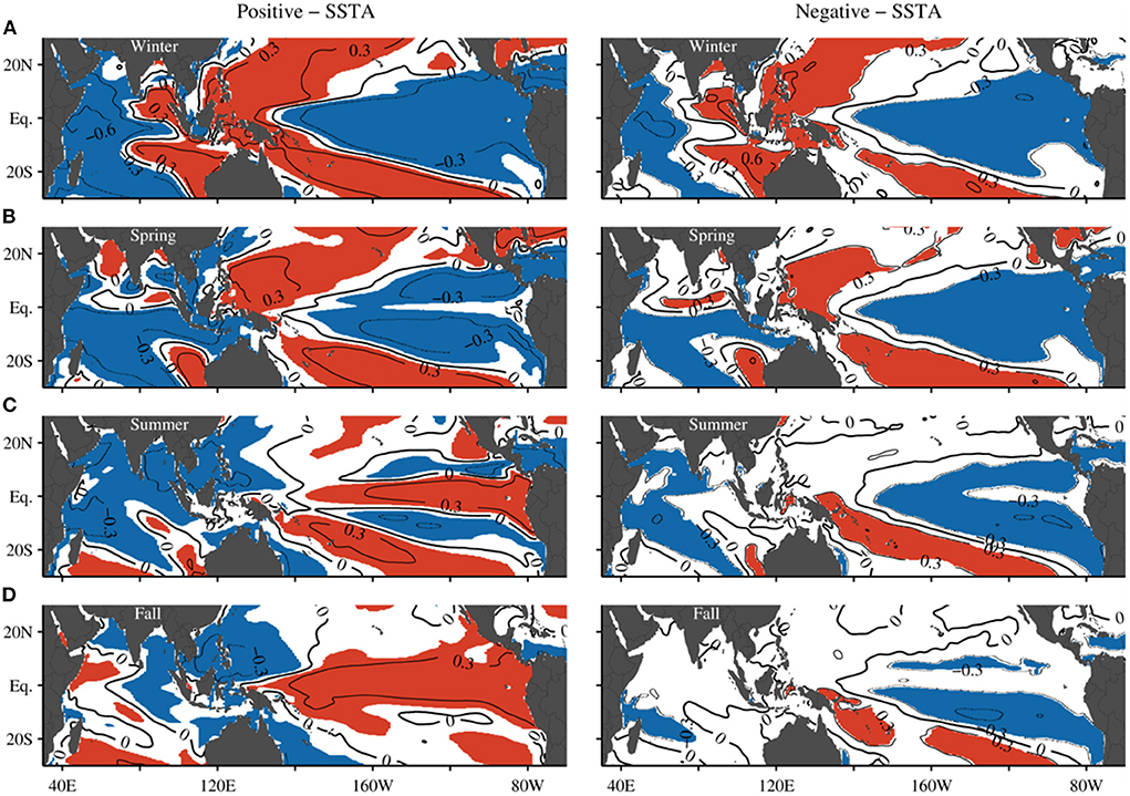
Figure 11. Comparison of lag correlations between the SSTA in STIO in fall and the tropical Indo-Pacific SSTA in the following four seasons for the positive (left column) and negative (right column) phases of the decadal variability in the CCSM4 historical simulations. (A) Winter (December to February). (B) Spring (March to May). (C) Summer (June to August). (D) Autumn (September to November). The contour interval is 0.3. Red and blue shades indicate 99% confidence level of positive and negative correlation, respectively.

Similar differences are also identified between the SSHA lag correlations in the positive and negative phases of the decadal variability, with similar lag correlations between the SSHA in STIO in fall and the tropical Indo-Pacific SSHA in the following winter, but significantly different lag correlations between the SSHA in STIO in fall and the cold tongue SSHA in the following spring through fall of Year +1 (Figure 12). The differences are because the thermocline in the cold tongue is deeper during the negative phases than during the positive phases of the decadal variability (Figure 13), so that the SSTA are less dictated by the oceanic channel dynamics. The decoupling of the SSTA with the thermocline anomalies results in weakened lag correlations in the cold tongue at the 1-year time lag.

FIGURE 12

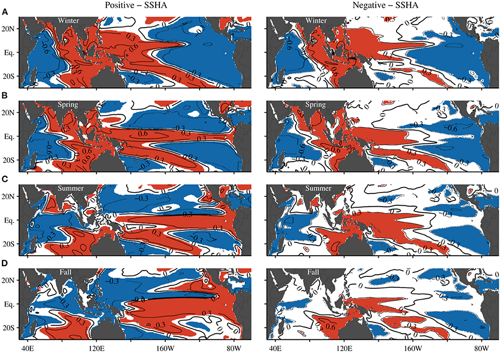
Figure 12. Comparison of lag correlations between the SSHA in STIO in fall and the tropical Indo-Pacific SSHA in the following four seasons during the positive (left column) and negative (right column) phases of the decadal variability in the CCSM4 historical simulations. (A) Winter (December to February). (B) Spring (March to May). (C) Summer (June to August). (D) Autumn (September to November). The contour interval is 0.3. Dark and light shades indicate 99% confidence level of positive and negative correlation, respectively.

FIGURE 13

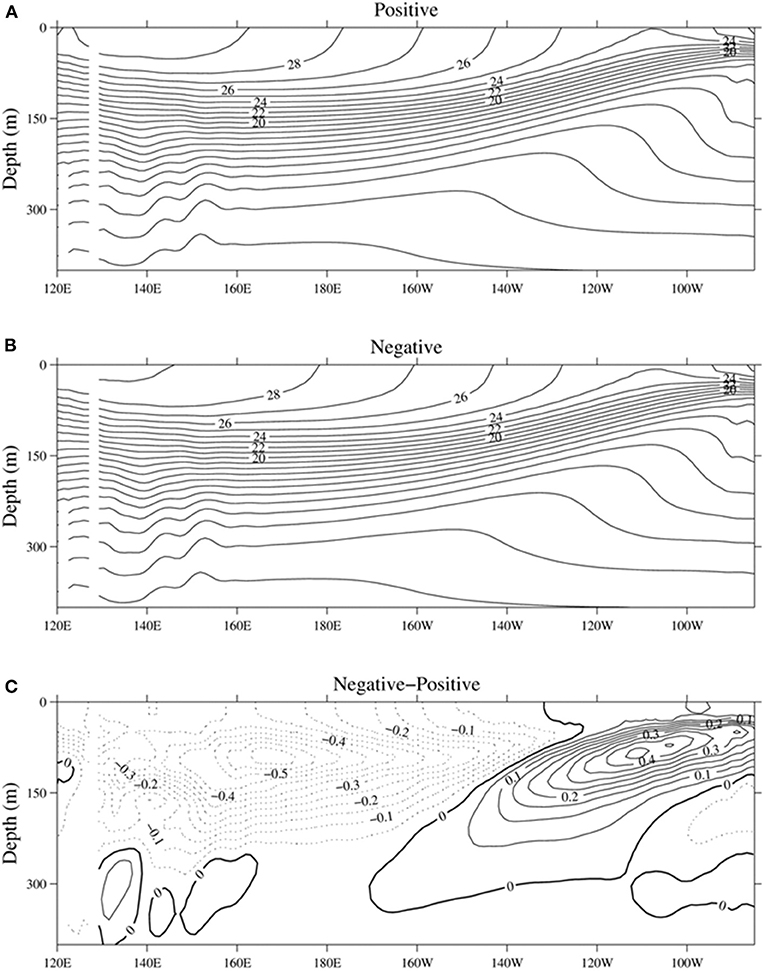
Figure 13. Comparison of the mean vertical temperature distribution in the equatorial Pacific vertical section during the positive (A) and negative (B) phases of the decadal variability in the CCSM4 historical simulations. (C) Is the difference of (B,A). Unit is °C.

The overestimated atmospheric bridge processes have been identified both in the positive and negative phases of the decadal variability (Figure 14), with similar patterns of significant lag correlations between the SZWA in the far western equatorial Pacific and the SZWA in the central equatorial Pacific, which are not supported by the observational analyses (Figure 9). Therefore, the model deficiencies are suggested to prevail in both the positive and negative phases of the decadal variability.

FIGURE 14

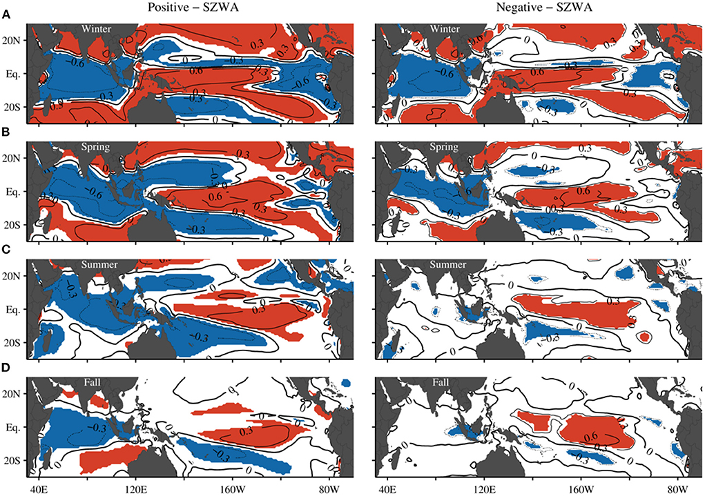
Figure 14. Comparison of lag correlations between the SZWA over the far western equatorial Pacific in fall and the tropical Indo-Pacific SZWA in the following four seasons during the positive (left column) and negative (right column) phases of the decadal variability in the CCSM4 historical simulations. (A) Winter (December to February). (B) Spring (March to May). (C) Summer (June to August). (D) Autumn (September to November). The contour interval is 0.3. Red and blue shades indicate 99% confidence level of positive and negative correlation, respectively.

The effects of the anthropogenic forcing on the decadal variability of the IOD-ENSO lag teleconnection is investigated using the historicalNat ensemble experiments in comparison with the results in the historical simulation experiments. The lag correlations of SSTA in STIO in fall with the SSTA over the Indo-Pacific Ocean in the following year or so are nearly unchanged during the positive and the negative phases of the decadal variability (Figures 11A,D, 15A,B). The correlations between SSHA in STIO in fall and the cold tongue SSHA at the one-year lag are also nearly unchanged during both phases of the decadal variability (Figures 12A,D, 15C,D), which are consistent with the SSTA lag correlations. The oceanic channel dynamics of the Indo-Pacific Ocean still prevail in the historicalNat experiments. The comparisons suggest that the anthropogenic forcing has small effects on the IOD-ENSO teleconnection.

FIGURE 15

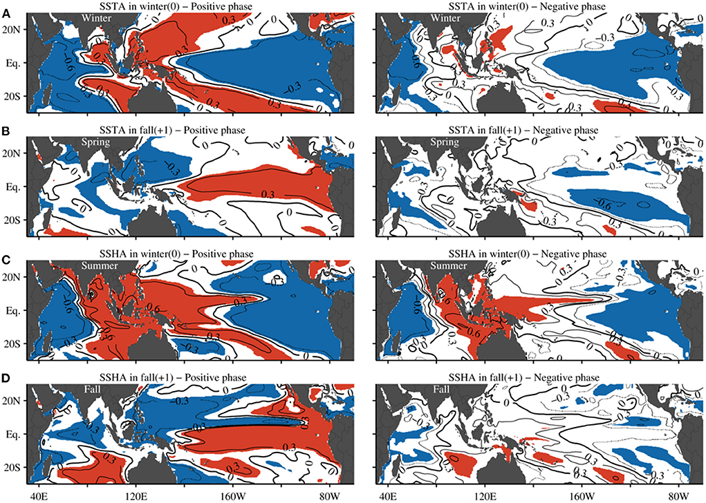
Figure 15. Comparison of lag correlations between the SSTA or SSHA in STIO in fall and the tropical Indo-Pacific SSTA or SSHA during the positive (left column) and negative (right column) phases of the decadal variability in the CCSM4 historicalNat simulations. (A) Lag correlations of SSTA in the winter of Year 0. (B) Lag correlations of SSTA in the fall of Year +1. (C) Lag correlations of SSHA in the winter of Year 0. (D) Lag correlations of SSHA in the fall of Year +1. The contour interval is 0.3. Red and blue shades indicate 99% confidence level of positive and negative correlation, respectively.

Conclusions

Based on lag correlation analyses of the observed and simulated SSTA in running windows of 7–11 years, the decadal variability of the IOD-ENSO precursory relation at the one-year time lag is identified. The dynamics of the IOD-ENSO precursory relation during the positive phases of the decadal variability are investigated using lag correlations of the CCSM4 climate system model experiments that participate in the CMIP5 project. The model experiments are shown to simulate the observed periodicity and spatial patterns of the ENSO events well. The simulated periodicity of IOD events still has sizable deviations from the observations. However, the spatial pattern and the correlation between ENSO and IOD have been simulated faithfully by the CCSM4 experiments, suggesting that the dynamics of the IOD-ENSO precursory relation can be investigated using the model experiments as a proxy.

The model has reproduced well the significant lag correlations between the SSTA in STIO in fall and the SSTA in the cold tongue in the eastern equatorial Pacific 1 year later during the positive phases of the decadal variability, in agreement with the observational analyses. The propagation of positive lag correlations, generated by the propagation of the SSHA anomalies from STIO to the Indonesian seas, inducing ITF transport anomalies and subsurface temperature anomalies in the western equatorial Pacific Ocean, are also simulated well by the model. The propagation of the SSHA lag correlations across the Indo-Pacific basins and the significant lag correlations between the STIO and the eastern Pacific oceanic anomalies are consistent with the observational analyses. The precursory relation between IOD and ENSO at the one-year time lead is due to the oceanic channel dynamics through the Indonesian Seas, namely the ITF variability.

The CCSM4 experiments are found to produce stronger lag correlations between the STIO and the eastern equatorial Pacific oceanic anomalies and over a larger longitudinal domain in the central-eastern equatorial Pacific than the observational analyses have suggested. In contrast, the simulated interannual anomalies of ITF geostrophic transport are noticeably smaller than the observed across the IX1 section in STIO. Analyses have shown that the difference is due to unrealistic westerly wind anomalies over the western-central equatorial Pacific in the year following IOD in the CCSM4 simulations, which generate unrealistic downwelling Kelvin waves in the western equatorial Pacific to propagate to the east and produce the higher lag correlations between the SZWA in the far western equatorial Pacific and the cold tongue SSTA at the 1 year time lag in the model than in the observations.

The lag correlations in the observations have shown that the SZWA in the far western equatorial Pacific that bottleneck the Walker Cell interactions over the Indian and the Pacific Oceans do not have significant correlations with the Pacific anomalies at the one-year time lag, suggesting that the so-called atmospheric bridge is not the primary process that control the IOD-ENSO precursory relation at the one-year time lag. The unrealistic lag correlations in the CCSM4 simulations between the SZWA in the far western equatorial Pacific and those in the cold tongue at the one-year time lag suggest model deficiency in simulating the atmospheric bridge processes. The analyses thus suggest that the CCSM4 experiments have underestimated the oceanic channel dynamics and overestimated the atmospheric bridge.

The dominance of the oceanic channel dynamics over the predictability of ENSO at the one-year lead time underlines the importance of simulating the ITF interannual transport anomalies correctly in climate system models. The analyses of this study suggest that the CCSM4 model needs to be improved to simulate realistic ITF transport anomalies. Higher spatial resolution and less diffusion of the model might be the remedy. In addition, the model has evidently produced an unrealistic atmospheric connection between the tropical Indian and the Pacific Oceans. Rectification of this error across the Indonesian maritime continent is needed to improve the model skills of simulating and predicting ENSO.

Data availability statement

The HadISST sea surface temperature data are available at https://www.metoffice.gov.uk/hadobs/hadisst/data/download.html. The AVISO sea surface height data are available at http://www.aviso.altimetry.fr/duacs. The Twentieth Century Reanalysis Project version 3 (20CRv3) dataset is provided by the U.S. Department of Energy, Office of Science Biological and Environmental Research (BER), by the National Oceanic and Atmospheric Administration Climate Program Office, and by the NOAA Physical Sciences Laboratory at https://psl.noaa.gov/data/gridded/data.20thC_ReanV3.html. The EN4 quality controlled ocean data (EN.4.2.1) is provided by the Met Office Hadley Center at https://www.metoffice.gov.uk/hadobs/en4/download-en4-2-1.html. The CMIP5 output data are available at https://esgf-node.llnl.gov/projects/cmip5/.

Author contributions

DY conceptualized the research and drafted the manuscript. PX and TX executed the research. XZ processed the CCSM4 data. All authors contributed to the article and approved the submitted version.

Funding

This study was supported by the National Natural Science Foundation of China (41720104008), the National Key Research and Development Program of China (2020YFA0608800 and 2019YFC1509102), and the Strategic Priority Project of Chinese Academy of Sciences (XDB42000000). DY was supported by the Taishan Scholar Program, QMSNL (2018SDKJ0104-02), Shandong Provincial (U1606402), and the Kunpeng Outstanding Scholar Program of the FIO/NMR of China. TX was supported by the Marine S&T Fund of Shandong Province for Pilot National Laboratory for Marine Science and Technology (Qingdao) (2022QNLM010304). XZ was supported by NSFC (42175027).

Acknowledgments

We thank the CCSM4 climate modeling groups for producing and making available their model output, the Earth System Grid Federation (ESGF) for archiving the data and providing access, and the multiple funding agencies who support CMIP5 and ESGF.

Conflict of interest

The authors declare that the research was conducted in the absence of any commercial or financial relationships that could be construed as a potential conflict of interest.

Publisher's note

All claims expressed in this article are solely those of the authors and do not necessarily represent those of their affiliated organizations, or those of the publisher, the editors and the reviewers. Any product that may be evaluated in this article, or claim that may be made by its manufacturer, is not guaranteed or endorsed by the publisher.

References

Alexander, M. A., Bladé, I., Newman, M., Lanzante, J. R., Lau, N. C., and Scot, J. D. (2002). The atmospheric bridge: the influence of ENSO teleconnections on Air–Sea Interaction over the Global Oceans. J. Clim. 15, 2205–2231. doi: 10.1175/1520-0442(2002)015<2205:TABTIO>2.0.CO;2

CrossRef Full Text | Google Scholar

Clarke, A. J., and Gorder, S. V. (2003). Improving El Niño prediction using a space-time integration of Indo-Pacific winds and equatorial Pacific upper ocean heat content. Geophys. Res. Lett. 30:1399. doi: 10.1029/2002GL016673

CrossRef Full Text | Google Scholar

Craig, A. P., Vertenstein, M., and Jacob, R. (2012). A new flexible coupler for earth system modeling developed for CCSM4 and CESM1. Int. J. High Perform. Comput. Appl. 26, 31–42. doi: 10.1177/1094342011428141

CrossRef Full Text | Google Scholar

Deser, C., Phillips, A., Tomas, R., Okumura, Y., Alexander, M., Capotondi, A., et al. (2012). ENSO and pacific decadal variability in the community climate system model version 4. J. Clim. 25, 2622–2651. doi: 10.1175/JCLI-D-11-00301.1

CrossRef Full Text | Google Scholar

Gent, P. R., Danabasoglu, G., Donner, L. J., Holland, M. M., Hunke, E. C., Jayne, S. R., et al. (2011). The community climate system model version 4. J. Clim. 24, 4973–4991. doi: 10.1175/2011JCLI4083.1

CrossRef Full Text | Google Scholar

Hunke, E. C., and Lipscomb, W. H. (2008). CICE: The Los Alamos Sea Ice Model Documentation and Software User's Manual, Version 4 (Tech. Rep. No. LA-CC-06-012). Los Alamos National Laboratory.

Google Scholar

Izumo, T., Lengaigne, M., Vialard, J., Luo, J. J., Yamagata, T., and Madec, G. (2014). Influence of Indian Ocean Dipole and Pacific recharge on following year's El Niño: interdecadal robustness. Clim. Dyn. 42, 291–310. doi: 10.1007/s00382-012-1628-1

CrossRef Full Text | Google Scholar

Izumo, T., Vialard, J., Lengaigne, M., Montegut, C. D., Behera, S. K., Luo, J. J., et al. (2010). Influence of the state of the Indian Ocean Dipole on the following year's El Nino. Nat. Geosci. 3, 168–172. doi: 10.1038/ngeo760

CrossRef Full Text | Google Scholar

Kalnay, E., Kanamitsu, M., Kistler, R., Collins, W., Deaven, D., Gandin, L., et al. (1996). The NCEP-NCAR 40-Year Reanalysis Project. Bull. Am. Meteorol. Soc. 77, 437–471.

Google Scholar

Kaplan, A., Cane, M., Kushnir, Y., et al. (1998). Analyses of global sea surface temperature 1856-1991. J. Geophy. Res. 103, 567–589. doi: 10.1029/97JC01736

CrossRef Full Text | Google Scholar

Klein, S. A., Soden, B. J., and Lau, N. C. (1999). Remote sea surface temperature variations during ENSO: evidence for a tropical atmospheric bridge. J. Clim. 12, 917–932.

Google Scholar

Kug, J.S., Li, T., An, S.I., Kang, I.S., Luo, J.J., Masson, S., et al. (2006). Role of the ENSO–Indian Ocean coupling on ENSO variability in a coupled GCM. Geophys. Res. Lett. 33:L09710. doi: 10.1029/2005GL024916

CrossRef Full Text | Google Scholar

Lau, N. C., Leetmaa, A., Nath, M. J., and Wang, H. L. (2005). Influence of ENSO-Induced Indo-Western Pacific SST anomalies on extratropical atmospheric variability during the boreal summer. J. Clim. 18, 2922–2942. doi: 10.1175/JCLI3445.1

CrossRef Full Text | Google Scholar

Lau, N. C., and Nath, M. J. (2003). Atmosphere–Ocean Variations in the Indo-Pacific Sector during ENSO Episodes. J. Clim.16, 3–20. doi: 10.1175/1520-0442(2003)016<0003:AOVITI>2.0.CO;2

CrossRef Full Text | Google Scholar

Lawrence, D. M., Oleson, K. W., Flanner, M. G., Thornton, P. E., Swenson, S. C., Lawrence, P. J., et al. (2011). Parameterization improvements and functional and structural advances in version 4 of the Community Land Model. J. Adv. Model Earth Syst. 3. doi: 10.1029/2011MS00045

CrossRef Full Text | Google Scholar

Luo, J. J., Zhang, R. C., Behera, S. K., Masumoto, Y., Jin, F. F., Lukas, R., et al. (2010). Interaction between El Niño and Extreme Indian Ocean Dipole. J. Clim. 23:726–42. doi: 10.1175/2009JCLI3104.1

PubMed Abstract | CrossRef Full Text | Google Scholar

Meehl, G. A., and Bony, S. (2011). Introduction to CMIP5. Clivar Exch 16, 4–5.

Meyers, G. (1996). Variation of Indonesian Throughflow and the El Niño–Southern Oscillation. J. Geophys. Res. 101, 12255–12263. doi: 10.1029/95JC03729

CrossRef Full Text | Google Scholar

Meyers, G., Bailey, R., and Woorby, A. P. (1995). Geostrophic transport of Indonesian Throughflow. Deep-Sea Res. I 42, 1163–1174. doi: 10.1016/0967-0637(95)00037-7

CrossRef Full Text | Google Scholar

Neale, R. B., Richter, J., Park, S., Lauritzen, P. H., Vavrus, S. J., Rasch, P. J., et al. (2013). The mean climate of the Community Atmosphere Model (CAM4) in forced SST and fully coupled experiments. J. Clim. 26, 5150–5168. doi: 10.1175/JCLI-D-12-00236.1

CrossRef Full Text | Google Scholar

Rayner, N. A., Parker, D. E., Horton, E. B., Folland, C. K., Alexander, L. V., Rowell, D. P., et al. (2003). Global analyses of sea surface temperature, sea ice, and night marine air temperature since the late nineteenth century. J. Geophys. Res. 108, 4407. doi: 10.1029/2002JD002670

CrossRef Full Text | Google Scholar

Saji, N. H., Goswami, B. N., Vinayachandran, P. N., and Yamagata, T. (1999). A dipole mode in the tropical Indian Ocean. Nature 401, 360–363. doi: 10.1038/43854

PubMed Abstract | CrossRef Full Text | Google Scholar

Smith, R. D., Jones, P., Briegleb, B., Bryan, F., Danabasoglu, G., Dennis, J., et al. (2010). The Parallel Ocean Program (POP) Reference Manual (Tech. Rep. No. LAUR-10-01853). Los Alamos National Laboratory.

Smith, T. M., Reynolds, R. W., Peterson, T. C., and Lawrimore, J. (2008). Improvement to NOAA's historical merged Land-Ocean surface temperature analysis (1880-2006). J. Clim. 21, 2283–2296. doi: 10.1175/2007JCLI2100.1

CrossRef Full Text | Google Scholar

Taylor, K. E., Stouffer, R. J., and Meehl, G. A. (2012). An Overview of CMIP5 and the experiment design. Bull. Am. Meteorol. Soc. 93:485–98. doi: 10.1175/BAMS-D-11-00094.1

PubMed Abstract | CrossRef Full Text | Google Scholar

White, W. B. (1995). Design of a global observing system for gyre scale upper ocean temperature variability. Prog. Oceanogr. 36, 169–217. doi: 10.1016/0079-6611(95)00017-8

CrossRef Full Text | Google Scholar

Wijffels, S. E., and Meyers, G. (2004). An Intersection of Oceanic Waveguides: Variability in the Indonesian Throughflow Region. J. Phys. Oceanogr. 34, 1232–1253. doi: 10.1175/1520-0485(2004)034<1232:AIOOWV>2.0.CO;2

CrossRef Full Text | Google Scholar

Wijffels, S. E., Meyers, G., and Godfrey, J. S. (2008). A twenty year average of the indonesian throughflow: regional currents and the interbasin exchange. J. Phys. Oceanogr. 38, 1965–1978. doi: 10.1175/2008JPO3987.1

CrossRef Full Text | Google Scholar

Xu, T., and Yuan, D. L. (2015). Why does the IOD-ENSO teleconnection disappear in some decades? Chin. J. Oceanol. Limnol. 33, 534–544. doi: 10.1007/s00343-015-4044-7

CrossRef Full Text | Google Scholar

Xu, T., Yuan, D. L., Yu, Y., and Zhao, X. (2013). An assessment of Indo-Pacific oceanic channel dynamics in the FGOALS-g2 coupled climate system model. Adv. Atmos. Sci. 30, 997–1016. doi: 10.1007/s00376-013-2131-2

CrossRef Full Text | Google Scholar

Yuan, D., Hu, X., Xu, P., Zhao, X., Masumoto, Y., and Han, W. (2018). The IOD-ENSO precursory teleconnection over the tropical Indo-Pacific Ocean: Dynamics and long-term trends under global warming. J. Oceanol. Limnol. 36:4–19. doi: 10.1007/s00343-018-6252-4

CrossRef Full Text | Google Scholar

Yuan, D., Wang, J., Xu, T., Xu, P., Zhou, H., and Zhao, X. (2011). Forcing of the Indian Ocean Dipole on the Interannual Variations of the Tropical Pacific Ocean: Roles of the Indonesian Throughflow. J. Clim. 24, 3593–3608. doi: 10.1175/2011JCLI3649.1

CrossRef Full Text | Google Scholar

Yuan, D., Xu, P., and Xu, T. (2017). Climate variability and predictability associated with the Indo-Pacific Oceanic Channel Dynamics in the CCSM4 Coupled System Model. Chin. J. Oceanol. Limnol. 35, 23–38. doi: 10.1007/s00343-016-5178-y

CrossRef Full Text | Google Scholar

Yuan, D., Zhou, H., and Zhao, X. (2013). Interannual Climate Variability over the Tropical Pacific Ocean Induced by the Indian Ocean Dipole through the Indonesian Throughflow. J. Clim. 26, 2845–2861. doi: 10.1175/JCLI-D-12-00117.1

CrossRef Full Text | Google Scholar

Zhou, Q., Duan, W., Mu, M., and Feng, R. (2015). Influence of positive/negative Indian Ocean Dipole on Pacific ENSO through Indonesian Throughflow: Results from sensitivity experiment. Adv Atm Sci 32, 783–793. doi: 10.1007/s00376-014-4141-0

CrossRef Full Text | Google Scholar