Prediction Challenges From Errors in Tropical Pacific Sea Surface Temperature Trends

1. Introduction

Seasonal climate predictions of the tropical Pacific Ocean are made against the backdrop of a warming climate, and it is unclear to what extent they are impacted by trends. Assessments of prediction skill across the tropical Pacific Ocean tend to highlight the monthly-to-seasonal averages of anomalies of sea surface temperature (SST) and the El Niño-Southern Oscillation (ENSO) Niño regions in particular (e.g., Becker et al., 2014; Barnston et al., 2019; Johnson et al., 2019b; Tippett et al., 2019). Part of the reason for not assessing trends and their impacts in seasonal forecasts is the relatively short length of the period over which model reforecasts, or hindcasts, are available, which in turn reflects the availability and quality of historical datasets that are the basis for initialization and verification. Higher resolution datasets, which can be used to initialize climate models, are primarily satellite-based and extend back to the early 1980s. As a result many model hindcasts only extend back so far, particularly those that are used for real-time prediction, like the North American Multi-Model Ensemble (NMME; Kirtman et al., 2014). This past year, the NMME celebrated its tenth year in forecast operations, making monthly-to-seasonal predictions of SST, surface temperature, and surface precipitation each month for a forecast horizon of 9–12 months (Becker et al., 2022). As a result of this longevity in real-time, another 10 years was added to the record of NMME hindcasts, making an assessment of long-term linear trends increasingly viable and relevant. Here, we address the question: Do initialized climate predictions capture the observed linear trend in the tropical Pacific over the last ~40 years (1982–2020)? Further, to what extent do these trends influence the prediction skill of monthly-to-seasonal outlooks for ENSO and the tropical Pacific?

Linear trends of predicted SSTs over the span 1982–2014 were previously explored in Shin and Huang (2019). From a set of five NMME models, they showed that linear trends were too strongly positive in predictions, and this generally worsened with forecast lead time. As a result of errors that were biased positive in the Niño-3.4 index, they speculated that linear trends may have led to El Niño false alarms in 2012 and 2014, two El Niño events that were predicted by the models but then failed to materialize. The missed 2014/15 El Niño forecast, as well as the borderline El Niño in 2018 were also cases where the expected atmospheric response in tropical rainfall and winds ended up being surprisingly anemic in observations, leading to questions of why the atmosphere was failing to couple with the ocean (McPhaden, 2015; Johnson et al., 2019a; Santoso et al., 2019). Due to interest in these recent high profile cases, we revisit and update the linear trend estimates provided in Shin and Huang (2019), include newer NMME models, extend the analysis to precipitation, and apply skill metrics used in forecast validation studies.

Often long-term SST trends are examined within the context of future emission scenarios in the CMIP5/6 experiments. The CMIP5/6 ensemble means project positive trends in SST and precipitation across much of the equatorial Pacific, with maximum strength in the central and eastern basin (Yeh et al., 2012; Fredriksen et al., 2020). While CMIP data are not investigated as part of this study, the CMIP5/6 SST trend patterns are broadly similar to the trends found in Shin and Huang (2019). Further, it's noteworthy that the historical CMIP5/6 SST trends can vary from the observations. For instance, Karnauskas et al. (2009) demonstrated that the SST gradient across the tropical Pacific has strengthened over the period from 1880 to 2005, so that the western Pacific is warming at a greater rate than the eastern Pacific—opposite of the trends simulated in CMIP5/6. The reduced warming in the eastern Pacific was also supported in Seager et al. (2019) who showed that during 1958–2017 observed SST trends in Niño-3.4 were much more muted than the positive trends within CMIP5. The observed strengthening of the SST gradient is also supported by studies documenting an acceleration of the overlying Walker circulation over recent decades (L'Heureux et al., 2013; Sohn et al., 2013; Kociuba and Power, 2015; Chung et al., 2019).

The sign of trends still remains a matter of debate because the observational data going back further in time is of reduced quality (Deser et al., 2010) and is not entirely consistent among different datasets (Solomon and Newman, 2012; Coats and Karnauskas, 2017). Therefore, mismatches between models and observations could reflect sparse observational inputs that exist across the tropical Pacific prior to the last half of the twentieth century (Power et al., 2021). Also, the divergence between the observational trends and CMIP may also reflect differences due to internal variability (Bordbar et al., 2019; Chung et al., 2019). Others have noted that recent decades could reflect a negative state of the Interdecadal Pacific Oscillation (Watanabe et al., 2021; Wu et al., 2021) or warming of the Atlantic Ocean (McGregor et al., 2018), which would be associated with an increased occurrence of La Niña and negative trends in SSTs and rainfall across the tropical Pacific. Further, while the majority of models and the mean of CMIP5/6 project an El Niño-like trend, not all participating models do (e.g., Kohyama and Hartmann, 2017).

In contrast to the initialized predictions from the NMME, CMIP models are mostly uninitialized free runs and therefore are not constrained to match the observed evolution—rather this set of models and their related experiments are primarily used to estimate the forced response to anthropogenic climate change. Shin and Huang (2019) investigated whether greenhouse gases (GHG) could be contributing to SST trends in NMME models and compared their results to one model, CCSM3, which has fixed GHG concentrations from the year 1990, unlike the other NMME models which have varying GHGs. The CCSM3 model has a comparable bias in the linear trend with other NMME models, leading them to infer that the overly positive trends in tropical Pacific SSTs are not a result of changes in GHG. If GHGs are not behind why the models overdo SST trends then what are the sources of trend errors in the NMME models? Perhaps it is also possible that these sources of errors partially apply to CMIP models.

While a closer inspection of NMME trends will not resolve the debate over the sign of future trends across the tropical Pacific, the NMME provides a valuable testing ground for the performance of initialized climate models in a warming world. If the NMME trend errors continue then it may suggest higher uncertainty in the CMIP projections than is fully appreciated. Errors that arise due to errors in the linear trend may have implications for the prediction of ENSO and other tropical Pacific anomalies. In the sections that follow, we take a look again at SST trend errors and also examine to what extent they map onto errors in forecast skill of SST and precipitation anomalies. We focus on total SST, not anomalies, because overlying precipitation anomalies in the tropical Pacific respond to total SSTs. Finally, we take a closer look at El Niño false alarms to see if the hypothesis of Shin and Huang (2019) can be supported using the reforecast data.

2. Data

We examine the ensemble means from eight NMME models that span the 1982–2020 time period (Kirtman et al., 2014). This set includes three models from NOAA Geophysical Fluid Dynamics Lab (GFDL), GFDL-CM2p5-FLOR-A, GFDL-CM2p5-FLOR-B, and GFDL-CM2p1-aer04, two models from Environment and Climate Change Canada, CanCM4i and GEM-NEMO, the National Centers for Environmental Prediction (NCEP) CFSv2 model, the National Aeronautics and Space Administration (NASA) GOESS2S model, and the CCSM4 model run at the University of Miami RSMAS. Reforecast and real-time data is merged together to maximize the dataset length. The GOESS2S model has the shortest forecast time horizon which goes out to 9 months (leads 0.5–8.5), CFSv2 is run out to 10 months (leads 0.5–9.5), and all other models extend to 12 months lead time (leads 0.5–11.5). All of the models in this study include time varying greenhouse gas concentrations (Becker 2022, personal communication). Real-time forecast runs are typically initialized within the first week of the month. While a multi-model average is often formed using participating NMME models, here we keep the models separate to explore the relationships among models and their different biases and behavior. Anomalies are formed by removing the calendar month climatology based on the full 1982–2020 period.

Two of the NMME models, the CFSv2 and CCSM4 have a discontinuity in 1999 because of a shift in the data assimilation. The initial conditions for both models are taken from the NCEP Climate Forecast System reanalysis (CFSR), which experienced a jump when ATOVS satellite data were assimilated into the stream of data (Xue et al., 2011; Kumar et al., 2012). When forecast anomalies are created, this is often corrected by using two separate climatological periods (e.g., Barnston et al., 2019). In this study we do not correct the discontinuity in the interest of using the native model versions submitted to the NMME, but it is common practice to correct for this in operational prediction (e.g., Xue et al., 2013). As will be shown, these two models stand out for their immediate errors beginning at short lead times, indicating that the discontinuity is aliased into total SST and precipitation anomaly trend errors.

Forecast verification of SSTs is against monthly OISSTv2 from Reynolds et al. (2002) because of its higher spatial resolution, which better matches datasets used to initialize models in NMME. Verification of precipitation anomalies is based on the CPC Merged Analysis of Precipitation (CMAP)(Xie and Arkin, 1997). Data are re-gridded to 1° × 1° to match NMME forecast fields.

3. Results

3.1. Total SST Trend Errors and Biases

Across all calendar months, the observed linear trend pattern (expressed as the change in degrees Celsius over the 1982–2020 period) is characterized by a positive SST trend in the western tropical Pacific Ocean, with minimal or weak trends in the equatorial central and eastern Pacific Ocean (Figure 1). North of the equator, in the eastern Pacific, positive SST trends prevail, while negative trends are observed south of the equator near Peru and Chile. Figure 2 shows the error in the linear trend over all months between 1982 and 2020 for each forecast lead time (to summarize, 0.5-, 4.5-, and 8.5-month leads are displayed as separate panels). The NMME is composed of initialized models, which can drift from the observed initial conditions with lead time. For each forecast lead time, the linear trend is therefore computed over 468 months (12 months × 39 years). From Figure 2, there are significant positive errors in the central and eastern Pacific SST trend, especially at longer lead times, more clearly emerging in all models by the 4.5-month lead time. There are two exceptions, CCSM4 and CFSv2, whose positive trend errors notably arise in the earliest lead times, which reflects the jump in the initialization error that occurs in 1999. Thus, while the observed SST trend during this 39-year period is toward a stronger zonal gradient across the equatorial Pacific Ocean, the forecast models have largely been the reverse of the observed change, forecasting a flatter SST gradient, indicated by an overly positive trend in the central and eastern Pacific.

FIGURE 1

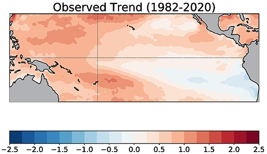
Figure 1. Linear trend of monthly sea surface temperature from January 1982 to December 2020. Units are in degrees Celsius change over January 1982 to December 2020. The thin gray lines indicate the equator and the International Date Line. Data is based on OISSTv2.

FIGURE 2

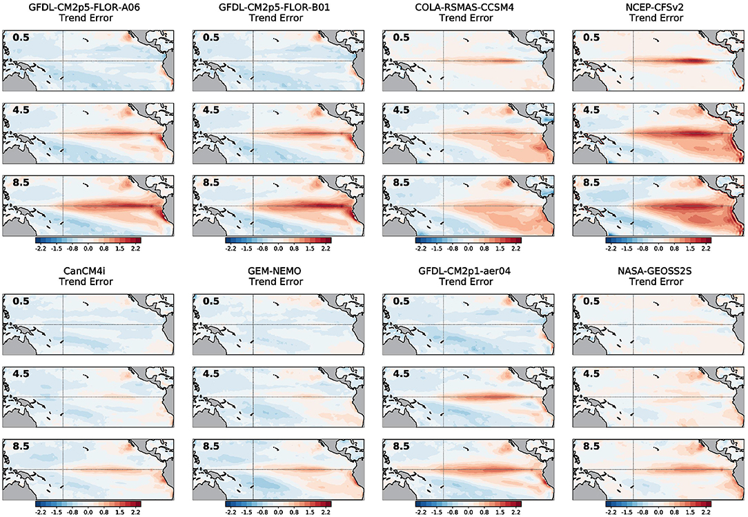
Figure 2. For each model in the NMME, linear trend error (forecasted coefficient minus observed coefficient) in monthly sea surface temperatures from January 1982 to December 2020. The bold number in each panel shows the forecast lead time (0.5-, 4.5-, and 8.5-month leads). Units are in the degrees Celsius change over January 1982 to December 2020. The thin gray lines indicate the equator and the International Date Line.

These errors in the total SST trend also result in trends in SST error over time, or as shown in Figure 3, trends in squared error. On the equator, the amplitude of the trend in the squared error tends to grow, in sync with the same forecast leads as the emergence of SST trend errors (compare with Figure 2). However, interestingly, the sign of the trend in squared error is not necessarily the same direction as the error in the SST trend. For instance, CM2p1-aer04 has a negative trend in squared error (Figure 3), while showing a clear positive error in the trend (Figure 2). This contrasts with the other two GFDL-provided models (FLORA-A06 and FLOR-B01), which have substantial positive trends in squared error. A change in sign can even occur within a single model. CFSv2 and CCSM4 show a negative trend in squared error in the eastern equatorial Pacific in the 0.5-month and 4.5-month leads, which flips to a positive trend by the 8.5-month lead time. So, despite the uniformly positive errors in the SST trend, what accounts for the varying sign of the trend in squared error?

FIGURE 3

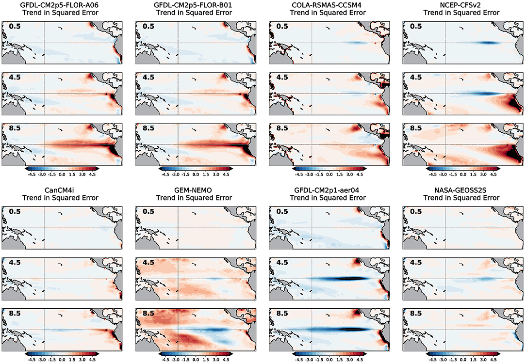
Figure 3. As in Figure 2 except showing the linear trend in the squared error of monthly sea surface temperatures from January 1982 to December 2020. Units are in degrees Celsius squared.

This apparent conundrum is resolved when the mean SST bias is examined for each model and lead times (Figure 4). The mean bias is simply the average forecast pattern minus the average observed pattern. Some NMME models, especially those shown in the panels of the top row, have a positive (warm) mean bias, again becoming more prominent at longer forecast lead times. Other NMME models, sorted into the panels of the bottom row, have a clear negative (cold) mean bias on the equator that also becomes more distinctive after the 4.5-month lead. The warm-biased models are associated with positive trends in squared error over time, and cold-biased models are related to negative trends in squared error over time. For CCSM4 and CFSv2, the mean bias gradually shifts from cold to warm with lead time (Figure 4) and, as such, the trend in the squared error reverses from predominantly negative to positive (Figure 3).

FIGURE 4

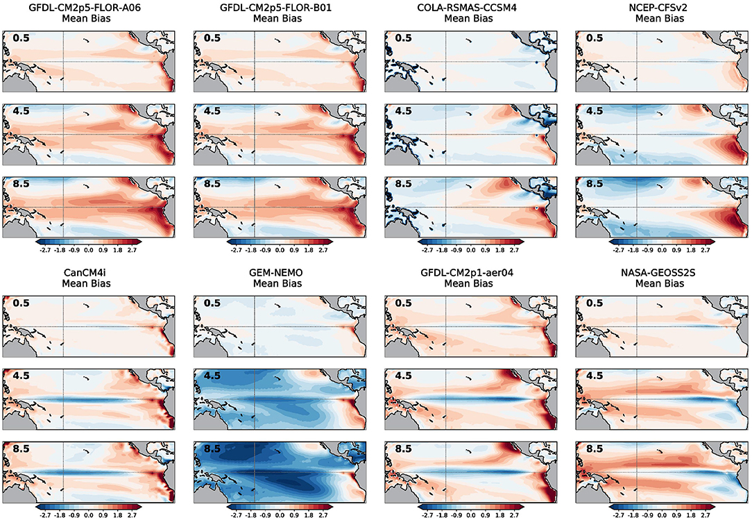
Figure 4. As in Figure 2 except showing the mean bias (forecast mean minus observed mean) in monthly sea surface temperatures over January 1982 to December 2020. Units are in degrees Celsius.

Forecast error is defined as the difference between the forecast and the observations, so in time a positive trend will shift a warm-biased model farther away from the observed state. Conversely, in time a positive trend will shift a cold-biased model increasingly nearer the observations. Thus, for forecast errors over time, cold-biased models will compensate for erroneously positive SST trends, but the same SST trend error will worsen forecast errors in warm-biased models.

Also, it appears to be the case that models that have a cold mean bias (bottom row of Figure 4) tend to also have weaker trend errors along the equator (bottom row of Figure 2). Likewise, models that have a warm mean bias (top row of Figure 4) tend to also have stronger trend errors (top row of Figure 2). The SST trend error also is more confined to the equator for cold-biased models compared to the warm-biased models, which more prominently extend south of the equator, reaching coastal Peru and Chile. This implies there is some relation between the amplitude of the trend error and the mean bias of the model, which will become more evident in the following section.

3.2. MSESS of Precipitation Anomalies and Its Relationship to SST Trend Errors

While the SST trend error and the trend in SST errors over time is concerning, it is common practice to remove the lead-dependent model mean climatology from forecasts to form an anomaly. It is these SST anomalies and their associated Niño region indices, that are the primary basis for monitoring and predicting ENSO. With the removal of the model climatology, the model's mean bias is removed throughout the seasonal cycle, as is part of the trend (when monthly starts are ignored as in this study), so the interpretation of errors in SST anomalies over the 1982–2020 record becomes considerably less straightforward. SST anomalies aside, total SSTs remains important for the formation of tropical convection and precipitation anomalies (e.g., He et al., 2018). These tropical Pacific precipitation anomalies are also tracked in association with ENSO because the displacement of tropical heating gives rise to global teleconnections, which ultimately result in climatic impacts in far flung regions. Thus, understanding these total SST trend errors on tropical precipitation anomalies is rather consequential.

To examine the influence of SST trend errors on precipitation anomalies, we start with an examination of the Mean Squared Error skill score (MSESS) for precipitation anomalies. Relative to other common metrics [e.g., mean squared error (MSE), root mean squared error (RMSE)] that evaluate the quality of the amplitude fit between the forecast anomaly f and the observation anomaly o, MSESS has the advantage of comparing the forecast MSE to the MSE of a climatological forecast, equivalently to the observed variance. Specifically,

$\text{MSESS}=1-\frac{{\text{MSE}}_{\text{fcst}}}{{\text{MSE}}_{\text{clim}}},$

where MSE_fcst is average over forecasts of (f − o)² and MSE_clim is the average of o², which is the observed variance since o is the observation anomaly. Tropical precipitation variance depends strongly on the region, with the western equatorial Pacific, near Indonesia, having higher variance than the eastern equatorial Pacific Ocean. Consequently, precipitation MSE (not shown) is largest in the western equatorial Pacific Ocean where it is easier for large forecast deviations to occur relative to the eastern Pacific where such swings are typically smaller. If the MSE of the forecast is less than variance of the observations, MSESS is positive, and the forecast is better than a climatological forecast. Otherwise, MSESS is negative, and the forecast is worse than a climatological forecast.

For short lead times, the predictions of precipitation anomalies are most skillful across the equatorial Pacific Ocean (Figure 5). However, at the 4.5-month lead, roughly the time when SST trend errors start to become prominent in the models (Figure 2), negative regions of MSESS are expanding, particularly in the eastern Pacific Ocean, at the expense of positive MSESS values, which are smaller and more restricted to the central Pacific. By the 8.5-month lead, positive values of MSESS are even more minimal. Interestingly, at this longer lead time, MSESS values appear to be slightly more positive on the equator for models in the bottom row of Figure 5 compared to models in the top row. Recall, these models in the bottom row of Figure 5 are the one that demonstrate weaker SST trend errors and a cold mean bias. Therefore, the MSESS of precipitation anomalies also reflects errors in the total SST fields.

FIGURE 5

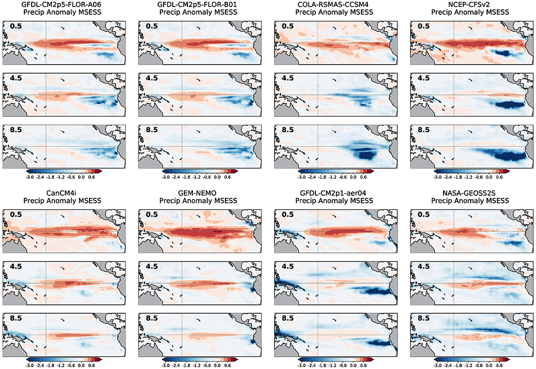
Figure 5. As in Figure 2 except showing the mean squared error skill score (MSESS) in precipitation anomalies from January 1982 to December 2020. Warm (cool) colors indicate forecast skill greater (less) than climatology. Values are unitless and range from minus infinity to one.

To simplify the presentation of results and further explore the relation of errors in precipitation anomalies with the total SST trend errors, we form indices (spatial averages) that are representative of the strongest correlations between total SSTs and precipitation anomalies. At each grid point, precipitation anomalies are correlated to the total SST, which results in the map shown in Figure 6 (left panel). The region with the largest correlations lies roughly in the central equatorial Pacific, so a precipitation anomaly index is formed by averaging precipitation anomalies bounded by 5°N-5°S, 170°E-140°W. This selected region also aligns well with the area that contains more skillful forecasts as measured by the MSESS (Figure 5). The region also matches the Central Pacific OLR index domain selected in L'Heureux et al. (2015), which was chosen because of strong coupling with SST anomalies. A SST index is then developed and is based on the correlation between the Central Pacific precipitation anomaly index and total SSTs at each grid point (Figure 6, right panel). The resulting total SST index is selected to include an area of maximum correlations (5°N-5°S, 180°-130°W) that is slightly shifted to the east of the precipitation anomaly index, which is consistent with previously documented relationships between SST and precipitation over the tropical Pacific Ocean (e.g., Gill and Rasmusson, 1983; Wang, 2000).

FIGURE 6

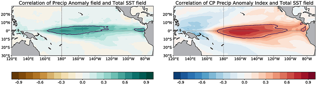
Figure 6. (Left) At each grid point, the correlation between total sea surface temperature and precipitation anomalies. (Right) The correlation between the Central Pacific precipitation anomaly index and total sea surface temperature at each grid point. The black contour shows the 95% level of significance using the effective degrees of freedom as estimated in Bretherton et al. (1999).

Some characteristics of these two indices are plotted for each NMME model and presented in the scatterplots shown in Figure 7. The x-axis displays the total SST trend index error (forecast trend minus observed trend) in degrees Celsius over the full period. The y-axis shows the MSESS of the Central Pacific precipitation anomaly index in the left panels and the RMSE in the right panels. The scatterplots shown in the two panels are similar, except for their orientation—larger RMSE values indicate less skill, while larger MSESS values indicate more skill. In the top panels of Figure 7, connecting lines are drawn between consecutive lead times for each model—dots oriented toward regions of less skill are associated with longer lead forecasts. In the bottom panels of Figure 7, the least-squares linear fit of precipitation skill and total SSST trend error between models is fit separately for each forecast lead time. In all of these panels, the strong relation between the total SST trend index error and the MSESS/RMSE in central Pacific precipitation anomalies really stands out. Larger, positive SST trend index errors are associated with lower skill in predicting the precipitation anomaly index. Interestingly, precipitation MSESS continues to increase for negative SST trend errors, which is suggestive of too wet precipitation forecasts even in the absence of positive SST trend errors. The correlation coefficient between these two quantities, over all models and lead times, is ~0.8 or ~64% explained variance (Figure 7, top panels).

FIGURE 7

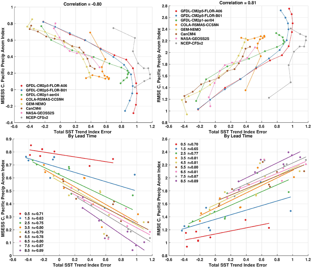
Figure 7. (Top Left) Scatterplot of mean squared error skill score (MSESS) of the central Pacific precipitation anomaly index on the y-axis and the error in the linear trend of the sea surface temperature index on the x-axis. (Top Right) Same as the left panel except showing the root mean squared error (RMSE) of the central Pacific precipitation anomaly index on the y-axis. (Bottom) Same as the top panels except also showing the least-squares fit for each forecast lead time. All forecast leads and NMME models are shown. The lines connect the forecast lead times, with smaller errors generally associated with shorter lead times. MSESS is unitless and is positive for forecasts whose MSE is less than the observed variance. RMSE is in units of millimeters/day. The SST trend index error is in units of degrees Celsius change over January 1982 to December 2020.

CFSv2 and CCSM4 are notably different from other models as they begin with larger SST trend index errors at shorter lead times and remain relatively constant. The initialization discontinuity in these two models also impacts the error in the precipitation anomalies, which generally increases with lead time. In this sense, these two models are more sensitive to the errors induced by the artificial jump in their initialization than they are to other processes that may arise in SST trend index errors. Excluding these two NMME models, the relationship between precipitation anomaly skill and SST trend error is larger (~0.9 or ~81% explained variance). The bottom panels of Figure 7 show that the slope steepens and correlations slightly increase with longer lead times. Despite this dependence on forecast lead time, even shorter lead times show substantial correlations between MSESS/RMSE of precipitation anomalies and SST trend error. Thus, these relations are not solely due to the drop in skill that occurs as the forecast increasingly departs from its initial condition.

3.3. Precipitation Anomaly Errors Explained by Linear Trend and Detrended SST Errors

We now consider the question of how much, over time, do the linear and detrended components of SST error explain errors in precipitation. Naturally, errors in SSTs do not completely explain errors in precipitation anomalies in the tropical Pacific. To assess how much precipitation error is explained by the two components of SST, we construct a 2-predictor multivariate linear regression:

$y=a{x}_1+b{x}_2+c$

In this regression, the predictors are the error in the time series of detrended SSTs (x₁) and the error in a time series of the least-squares linear fit (trend) through SSTs (x₂). The predictand y is the error in precipitation anomalies. The predictors and predictand are based on indices defined earlier in Figure 6, so that results from all models and lead times can be compactly summarized. The regression is re-computed separately for each forecast lead time and model.

The top panel of Figure 8 shows, on the vertical axis, the fraction of explained variance (in percent) of the 2-predictor regression. The horizontal axis displays the SST trend index error (as shown in Figure 7). The fraction of precipitation anomaly error variance explained by 2-predictor regression ranges from close to none to upwards of ~65%, with higher explained variance for models and lead times with larger SST trend index errors. Other than CFSv2 and CCSM4, shorter forecast lead times do not have a strong correlation between errors in SSTs and precipitation anomalies, but longer lead times have more of an association.

FIGURE 8

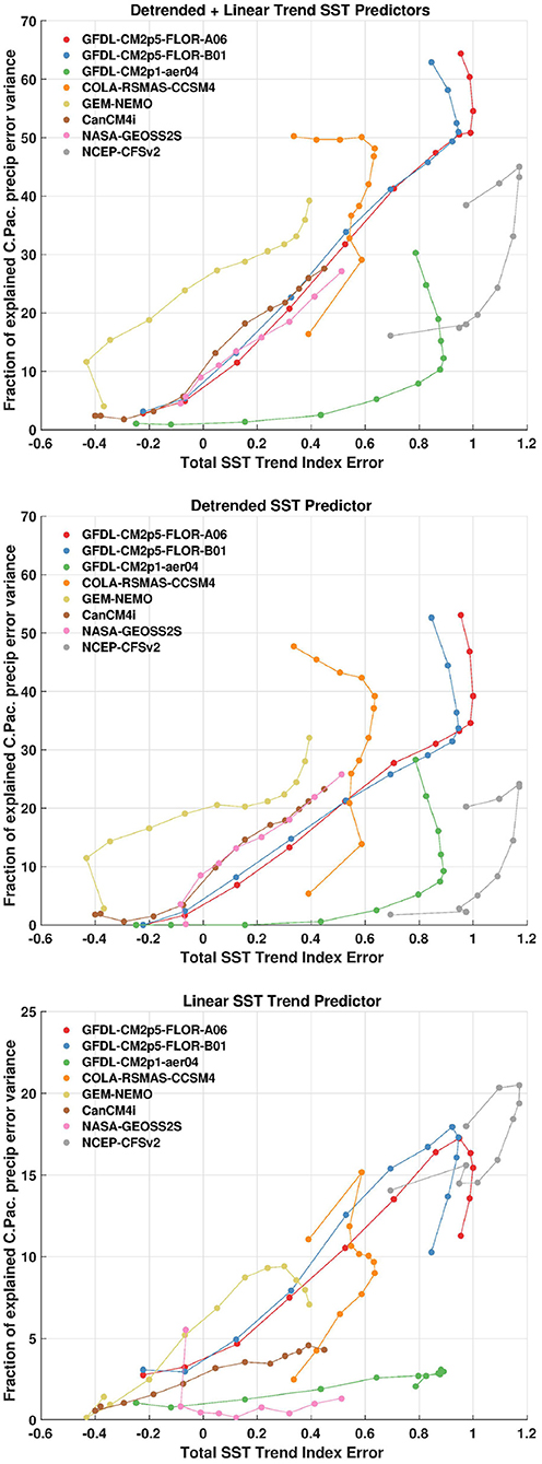
Figure 8. (Top) Correlation between the 2-predictor regression and the error in the central Pacific precipitation anomaly index. The predictors are the error in the detrended total SST index and the error in the least-squares linear fit through the SST index. The y-axis is expressed in terms of the percent of explained variance. (Middle) Correlation between the error in the detrended total SST index and error in the central Pacific precipitation anomaly index. (Bottom) Same as the middle panel except using the error in the least-squares linear fit through the SST index. All forecast leads and NMME models are shown. The SST trend index error is in units of degrees Celsius change over January 1982 to December 2020.

The fraction of precipitation anomaly error variance explained by the individual predictors (trend and detrended SST) are shown in the same format in the remaining panels of Figure 8. The detrended component of SST error accounts for most of the explained variance in precipitation errors (middle panel) relative to the trend component of SST errors (bottom panel; note the change in the y-axis). By construction, the explained variances shown in the lower two panels sum to the explained variance in the top panel since the individual predictors are uncorrelated. The trend component explains upwards of ~20% of the variability in precipitation error (and vice versa), while the detrended component accounts for up to ~50% of the variability. Thus, linear SST trend errors explain relatively little of the monthly variability of errors in precipitation anomalies. This suggests that SST trend errors are mostly problematic when predicting precipitation anomaly errors because of resulting deviations in amplitude (shown in Figure 7)—not due to issues with the phasing between SSTs and precipitation. Some models, such as GFDL-CM2p1-aer04 and NASA-GEOSS2S, have very little association between the errors in the SST trend component and precipitation anomalies at all lead times (Figure 8, bottom). However, the remaining models have stronger correlations, especially at longer lead times. The CCSM4, FLOR-A, FLOR-B, and CFSv2 models have the largest explained variances, which is also interesting in the context that these four models also tend to have a warmer mean bias than the other models (Figure 4).

The models and lead times that have larger explained variance between the SST trend errors and precipitation anomaly errors, are also the same models and lead times that have a clear relationship between trends in precipitation anomaly errors and trends in SSTs (Figure 9). In contrast to previous figures, Figure 9 displays the linear trends in precipitation anomaly errors on the y-axis. The overall similarity between the scatterplots in Figure 9 and the bottom panel of Figure 8 demonstrate the correlations in Figure 8 (bottom panel) arise in tandem with trends in errors of precipitation anomalies. In other words, linear SST errors can only be useful as a predictor for anomalous precipitation errors insofar as the latter also has linear trends. The least-squares linear regression, Figure 9 (bottom panel) shows that these relationships also endure as a function of forecast lead time and do not only exist by model.

FIGURE 9

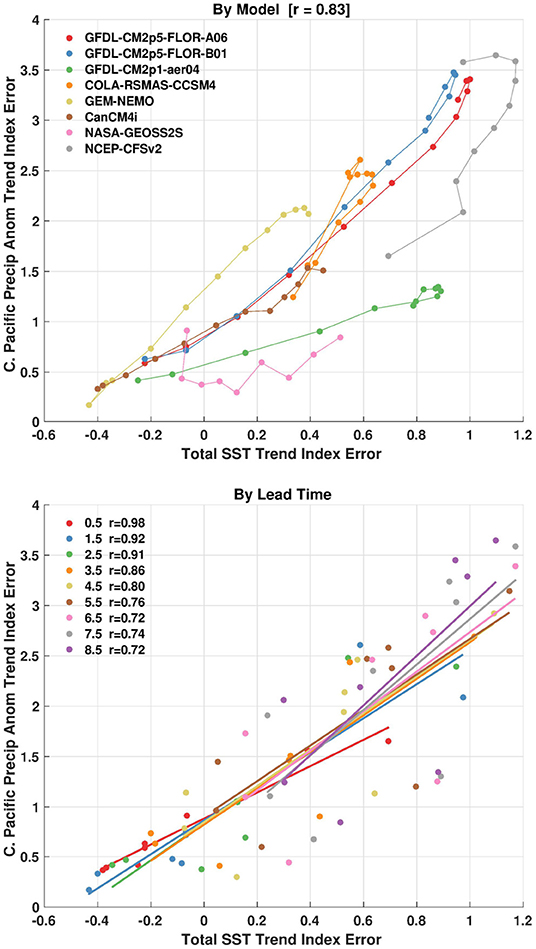
Figure 9. (Top) Scatterplot of error in the linear trend of Central Pacific precipitation anomaly index on the y-axis and the error in the linear trend of the total sea surface temperature index on the x-axis. The lines connect the forecast lead times, with smaller errors generally associated with shorter lead times. (Bottom) Same as the top panel except also showing the least-squares fit for each forecast lead time. All forecast leads and NMME models are shown.The index errors are in units of degrees Celsius (SST) and millimeters/day (precip) change over January 1982 to December 2020.

3.4. Relating Recent El Niño False Alarms With Errors in Trends of SST and Precipitation

To this point, we have shown that models and lead times with larger errors in SST trends are also linked to larger errors in precipitation anomalies. This is the case for forecast metrics evaluating amplitude errors and the quality of the fit between time series. For the latter metric, however, the linear trend SST component only explains up to ~20% of monthly variability in precipitation errors, and often much less. Regardless, models with larger errors in SST trends are also linked with larger errors in precipitation trends, which likely stems from the strongly coupled ocean-atmosphere system found across the tropical Pacific Ocean. Though the correlation of errors is not large for monthly variability, it appears there are substantial amplitude biases in precipitation anomalies. RMSE of central Pacific precipitation anomalies (Figure 7, right panels) which range from 1 mm/day (shortest lead) to 2–3 mm/day (longest leads), which is a large portion of typical daily mean precipitation in this region (3–5 mm/day). We've shown that the direction of these SST and precipitation errors are toward increasingly warmer SSTs and wetter precipitation anomalies.

What are the consequences of these increasing amplitude errors over time? One possible impact is on the occurrence of false alarms in El Niño prediction. These are El Niño events which are predicted by the models, but end up failing to occur in reality. Tippett et al. (2020) identified several El Niño false alarms while analyzing model “excessive momentum,” in which the observed Niño-3.4 SST index tendency during the spring is too strongly correlated with the forecast tendency of ENSO into the fall. In other words, positive springtime changes in the observed Niño-3.4 index often beget a positive forecast trajectory in the Niño-3.4 index. Tippett et al. (2020) showed that out of all springtime busts during 1982–2018, four of nine occurred in the last decade (2011, 2013, 2014, and 2017) and they were all El Niño false alarms–a concerning development for seasonal climate forecasting if it continues.

Excessive model momentum cannot be directly attributed to trend errors because it is computed as the difference of 1 month with following months, which eliminates the presence of trends. However, perhaps the uptick in the frequency of El Niño false alarms may have some roots in the linear SST and precipitation errors uncovered so far. In principle, model errors that tend to be warmer and wetter may be associated with more El Niño-like conditions and errors over time. To explore the idea that errors in trends could result in an increased number of El Niño false alarms, we generate a 100-member ensemble AR(2) model that mimics the characteristics of the observed Niño-3.4 SST index (Figure 10). The AR(2) model is:

$X_t={\varphi }_1{X}_{t-1}+{\varphi }_2{X}_{t-2}+ϵ,$

where X is the Niño-3.4 SST index and its subscript indicates the time in months, the AR parameters ϕ₁ and ϕ₂ are estimated by ordinary least squares using observed values of the Niño-3.4 index, and ϵ is white noise with variance equal to the error variance. The synthetic forecast signal is then computed using the derived AR(2) parameters. Members are then generated using a joint normal model as described in, for instance, Tippett et al. (2019). As in “perfect model,” we extract one member and call it the observations and then average the remaining members (ensemble mean). The resulting time series in Figure 10 (top panel) shows there are El Niño false alarms that arise due to unpredictable, intrinsic uncertainty in the forecast system. These false alarms are noted by the pink dots and the False Alarm Ratio (FAR) is computed as:

$\text{FAR}=M/N,$

where M is the number of months when the ensemble mean forecast exceeded the +0.45°C El Niño threshold and the observations did not. N is the total number of months. The FAR is also referred to as the probability of false alarm (Barnes et al., 2009). The false alarms occur throughout the time series, but tend to be clustered due to the persistence of the Niño-3.4 index. The introduction of a positive linear trend in the model simulation (here using the SST error found in FLOR-A at 8.5-month lead) increases the overall false alarm ratio in this particular example, but the most dramatic change is the shift of false alarms from the earlier part of the period to the later part (Figure 10, bottom panel).

FIGURE 10

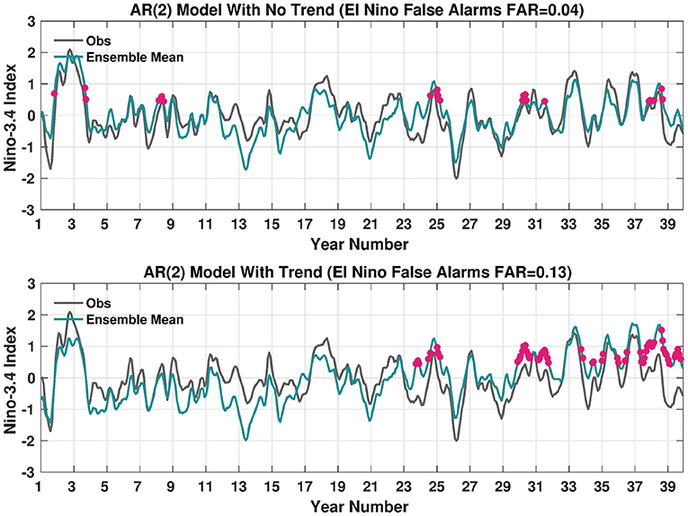
Figure 10. AR(2) Ensemble Mean Model Simulation of the Niño3.4 SST index (blue line) shown with no linear trend (Top) and with a linear trend that matches the trend in FLOR-A for lead = 8.5 (Bottom). The gray line, or observational proxy, is a single member from the 100-member simulation. Pink dots show the occurrence of El Niño False Alarms or cases when the Niño3.4 index prediction is in excess of 0.45°C, but the observations are less than this threshold. The simulation is in units of degrees Celsius.

This result therefore raises the possibility that increased frequency of El Niño false alarms may be tied to linear trend errors across the tropical Pacific. To explore whether we have seen similar shifts in NMME forecasts, Figure 11 shows the same scatterplots as in previous figures except showing false alarms for the full 1982–2020 record in the top panel, the post-2000 record in the middle panel, and the pre-2000 record in the bottom panel. The scatterplots show that there is a strong positive relation between El Niño FAR and the error in SST trends over the entire record, and that the error is almost exclusively found in forecasts made after 2000. If CCSM4 and CFSv2 are removed due to their unique initialization problems, the correlations in the scatterplot increase from r = 0.61 to r = 0.81 over the entire record (Figure 11, top panel) and increase from r = 0.82 to r = 0.93 in the post-2000 record (Figure 11, middle panel). These high correlations in the latter half of the record strongly suggests that El Niño false alarms have become more frequent due to linear SST trend errors. Prior to 2000, SST trend errors have little impact (Figure 11, bottom panel) compared to recent record, which is characterized by significant amplitude errors resulting in a too warm (and too wet) tropical Pacific Ocean.

FIGURE 11

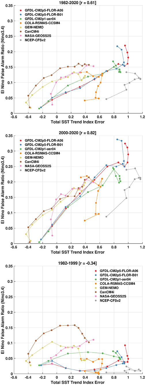
Figure 11. (Top) For the entire 1982–2020 period, scatterplot of the El Niño False Alarm Ratio in NMME (using a +0.5C threshold in the Niño-3.4 SST index) on the y-axis, along with the error in the linear trend of the total sea surface temperature index on the x-axis. (Middle) Same as top panel except for false alarms during 2000–2020. (Bottom) Same as top panel except for false alarms during 1982–1999. All forecast leads and NMME models are shown. The SST trend index error is in units of degrees Celsius change over January 1982 to December 2020.

4. Discussion

Over the span 1982–2020, the NMME models demonstrate significant positive errors in the linear trend of tropical Pacific SST that becomes more pronounced with lead time (Figure 2), confirming the result of Shin and Huang (2019) who used a subset of models. We further show that there is also a corresponding trend in squared errors in SSTs (Figure 3), and the sign of the trend in error is a function of the mean bias of the model and lead time (Figure 4). Models with a warm mean bias show increasing errors over time because the positive linear trend errors diverge more strongly from observations. The opposite is true for models with a cold mean bias, which show decreasing errors over time because the positive trend helps close the gap with the observations. Models and lead times with more severe SST trend errors are also associated with larger errors and lower skill in equatorial Central Pacific precipitation anomalies (Figures 5, 7, 8). However, the trend SST component only describes a small percentage of variability in precipitation errors (Figure 8), meaning that the linear trend is not particularly useful to predict the month-to-month variability in precipitation errors. However, the RMSE (Figure 7), or errors in the amplitude, is quite large as a percent of typical climatology. It is these errors in amplitude that ultimately arise in an increased frequency of El Niño false alarms, which has become more evident in the latter half of the ~40 year record (Figure 11).

Detrending removes errors associated with the linear trend. Figure 12 (left panel) shows the MSESS for the previously defined total SST index (top row) and precipitation anomaly index (bottom row) for all models and lead times. The middle panel of Figure 12 shows the scores for detrended indices and the right panel reveals the difference in MSESS between the two leftmost panels. A sign test is applied to the difference and shading is only shown where differences are statistically significant at the 95% level. From this figure, we can see that linearly detrending the data improves the prediction skill for a subset of models, namely only those models that have clear warm biases and more pronounced trend errors as identified in Section 3.1. While not shown here, the El Niño false alarm ratio also decreases for detrended data, though it is not eliminated. Though linearly detrending the data provides an increase in skill retrospectively, there are additional challenges with applying the linear trend corrections to models in real time. Mainly, as van Oldenborgh et al. (2021) discussed in their study on defining ENSO indices in a warming climate, the warming trend has accelerated in the last 50 years, so trends estimated on past data may not hold for future data. Identifying trends is therefore a challenge when trying to make predictions for the future.

FIGURE 12

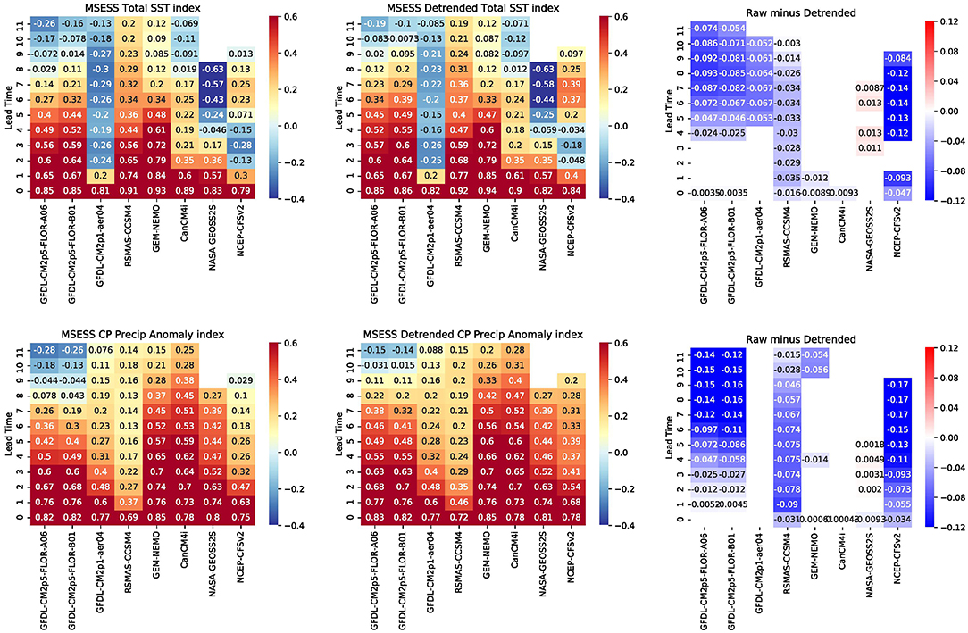
Figure 12. (Top) Heat map of Mean Squared Error Skill Score (MSESS) for the total SST index, including the (left panel) SST trend (middle panel) and for linearly detrended SSTs and (right panel) difference between the left and right panels. (Bottom) Same as the top row except for the central Pacific precipitation anomaly index. Shading is only shown where differences are statistically significant at the 95% level. MSESS is unitless and is positive for forecasts whose MSE is less than the observed variance.

Why do these linear SST errors arise? One can only speculate based on the results presented here, but while differences in the 40 year linear trend between the observations and CMIP5/6 models can be attributed to internal variability masking the forced trend (Olonscheck et al., 2020), such a reason cannot be applied to NMME models. Thus, one possibility is that errors associated with model physics may result in linear trend errors in SSTs and precipitation anomalies. Indeed this reason has been explored by others searching for a reason for the divergence between trend in observations and CMIP models. For example, it has been observed that the models project too much upper-tropospheric warming (Po-Chedley and Fu, 2012; Mitchell et al., 2020). As Sohn et al. (2016) point out, too much upper-level warming would act to weaken the overturning Walker circulation (also weakening the SST gradient). They demonstrate that models with a weaker Walker circulation are also models with static stability that is too strong and speculate that issues with convective parameterizations may be the root of this disparity (e.g., Tomassini, 2020). Others have discussed potential errors in ocean physics as well, contributing to an amplified surface heat flux feedback that may result in too much warming in the cold tongue region of the eastern Pacific (e.g., Seager et al., 2019).

There are several other avenues to be explored in the future. One path is to examine the seasonality of linear trends and their errors since they may be worse during certain seasons. For example, ENSO prediction already suffers from low skill for spring starts, and trend errors might further hinder skill during this period. Another path is to investigate errors associated with La Niña. While problems with the linear trend in SSTs can lead to El Niño false alarms, it is conceivable that La Niña events are similarly underestimated and under-predicted. van Oldenborgh et al. (2021) noted that linear trend removals are not adequate for ENSO monitoring and that positive trends in SSTs have been masking recent La Niña events, which have stronger amplitude and impacts than originally assumed. Finally, because total SSTs have a strong relationship with overlying tropical precipitation anomalies, what are the consequences for subsequent ENSO teleconnections and global impacts? Predictions of the tropical Pacific are a primary basis for seasonal predictions outside of the tropics and such trend errors may have knock-on impacts that should be investigated.

Data Availability Statement

The NMME model data analyzed for this study can be found in the International Research Institute for Climate and Society data library at https://iridl.ldeo.columbia.edu/SOURCES/.Models/.NMME/.

Author Contributions

All authors listed have made a substantial, direct, and intellectual contribution to the work and approved it for publication.

Conflict of Interest

The authors declare that the research was conducted in the absence of any commercial or financial relationships that could be construed as a potential conflict of interest.

Publisher's Note

All claims expressed in this article are solely those of the authors and do not necessarily represent those of their affiliated organizations, or those of the publisher, the editors and the reviewers. Any product that may be evaluated in this article, or claim that may be made by its manufacturer, is not guaranteed or endorsed by the publisher.

Acknowledgments

We thank two reviewers, Arun Kumar (NOAA CPC), and Dan Harnos (NOAA CPC) for their careful and constructive reviews.

References

Barnes, L. R., Schultz, D. M., Gruntfest, E. C., Hayden, M. H., and Benight, C. C. (2009). Corrigendum: false alarm rate or false alarm ratio? Weather Forecast. 24, 1452–1454. doi: 10.1175/2009WAF2222300.1

CrossRef Full Text | Google Scholar

Barnston, A. G., Tippett, M. K., Ranganathan, M., and L'Heureux, M. L. (2019). Deterministic skill of ENSO predictions from the North American multimodel ensemble. Clim. Dyn. 53, 7215–7234. doi: 10.1007/s00382-017-3603-3

PubMed Abstract | CrossRef Full Text | Google Scholar

Becker, E., van den Dool, H., and Zhang, Q. (2014). Predictability and forecast skill in NMME. J. Clim. 27, 5891–5906. doi: 10.1175/JCLI-D-13-00597.1

CrossRef Full Text | Google Scholar

Becker, E. J., Kirtman, B. P., L'Heureux, M., Munoz, A. G., and Pegion, K. (2022). A decade of the north american multi-model ensemble (NMME): Research, application, and future directions. Bull. Amer. Meteor. Soc. doi: 10.1175/BAMS-D-20-0327.1

CrossRef Full Text | Google Scholar

Bordbar, M. H., England, M. H., Sen Gupta, A., Santoso, A., Taschetto, A. S., Martin, T., et al. (2019). Uncertainty in near-term global surface warming linked to tropical Pacific climate variability. Nat. Commun. 10, 1990. doi: 10.1038/s41467-019-09761-2

PubMed Abstract | CrossRef Full Text | Google Scholar

Bretherton, C. S., Widmann, M., Dymnikov, V. P., Wallace, J. M., and Blade, I. (1999). The effective number of spatial degrees of freedom of a time-varying field. J. Clim. 12, 1990–2009. doi: 10.1175/1520-0442(1999)012<1990:TENOSD>2.0.CO;2

CrossRef Full Text | Google Scholar

Chung, E.-S., Timmermann, A., Soden, B. J., Ha, K.-J., Shi, L., and John, V. O. (2019). Reconciling opposing Walker circulation trends in observations and model projections. Nat. Clim. Change 9, 405–412. doi: 10.1038/s41558-019-0446-4

CrossRef Full Text | Google Scholar

Coats, S., and Karnauskas, K. B. (2017). Are simulated and observed twentieth century tropical Pacific sea surface temperature trends significant relative to internal variability? Geophys. Res. Lett. 44, 9928–9937. doi: 10.1002/2017GL074622

CrossRef Full Text | Google Scholar

Deser, C., Alexander, M. A., Xie, S.-P., and Phillips, A. S. (2010). Sea surface temperature variability: patterns and mechanisms. Annu. Rev. Mar. Sci. 2, 115–143. doi: 10.1146/annurev-marine-120408-151453

PubMed Abstract | CrossRef Full Text | Google Scholar

Fredriksen, H.-B., Berner, J., Subramanian, A. C., and Capotondi, A. (2020). How does El Ni o-Southern Oscillation change under global warming-A first look at CMIP6. Geophys. Res. Lett. 47, e2020GL090640. doi: 10.1029/2020GL090640

CrossRef Full Text | Google Scholar

Gill, A. E., and Rasmusson, E. M. (1983). The 1982-83 climate anomaly in the equatorial Pacific. Nature 306, 229–234. doi: 10.1038/306229a0

CrossRef Full Text | Google Scholar

He, J., Johnson, N. C., Vecchi, G. A., Kirtman, B., Wittenberg, A. T., and Sturm, S. (2018). Precipitation sensitivity to local variations in tropical sea surface temperature. J. Clim. 31, 9225–9238. doi: 10.1175/JCLI-D-18-0262.1

CrossRef Full Text | Google Scholar

Johnson, N. C., L'Heureux, M. L., Chang, C.-H., and Hu, Z.-Z. (2019a). On the delayed coupling between ocean and atmosphere in recent weak El Nino episodes. Geophys. Res. Lett. 46, 11416–11425. doi: 10.1029/2019GL084021

CrossRef Full Text | Google Scholar

Johnson, S. J., Stockdale, T. N., Ferranti, L., Balmaseda, M. A., Molteni, F., Magnusson, L., et al. (2019b). Seas5: the new ECMWF seasonal forecast system. Geosci. Model Dev. 12, 1087–1117. doi: 10.5194/gmd-12-1087-2019

CrossRef Full Text | Google Scholar

Karnauskas, K. B., Seager, R., Kaplan, A., Kushnir, Y., and Cane, M. A. (2009). Observed strengthening of the zonal sea surface temperature gradient across the equatorial Pacific ocean. J. Clim. 22, 4316–4321. doi: 10.1175/2009JCLI2936.1

CrossRef Full Text | Google Scholar

Kirtman, B. P., Min, D., Infanti, J. M., Kinter, J. L., Paolino, D. A., Zhang, Q., et al. (2014). The North American Multimodel Ensemble: Phase-1 seasonal-to-interannual prediction; phase-2 toward developing intraseasonal prediction. Bull. Am. Meteorol. Soc. 95, 585–601. doi: 10.1175/BAMS-D-12-00050.1

CrossRef Full Text | Google Scholar

Kociuba, G., and Power, S. B. (2015). Inability of CMIP5 models to simulate recent strengthening of the Walker circulation: implications for projections. J. Clim. 28, 20–35. doi: 10.1175/JCLI-D-13-00752.1

CrossRef Full Text | Google Scholar

Kohyama, T., and Hartmann, D. L. (2017). Nonlinear ENSO warming suppression (NEWS). J. Clim. 30, 4227–4251. doi: 10.1175/JCLI-D-16-0541.1

CrossRef Full Text | Google Scholar

Kumar, A., Chen, M., Zhang, L., Wang, W., Xue, Y., Wen, C., et al. (2012). An analysis of the nonstationarity in the bias of sea surface temperature forecasts for the NCEP Climate Forecast System (CFS) version 2. Monthly Weather Rev. 140, 3003–3016. doi: 10.1175/MWR-D-11-00335.1

CrossRef Full Text | Google Scholar

L'Heureux, M. L., Lee, S., and Lyon, B. (2013). Recent multidecadal strengthening of the Walker circulation across the tropical Pacific. Nat. Clim. Change 3, 571–576. doi: 10.1038/nclimate1840

CrossRef Full Text | Google Scholar

L'Heureux, M. L., Tippett, M. K., and Barnston, A. G. (2015). Characterizing ENSO coupled variability and its impact on North American seasonal precipitation and temperature. J. Clim. 28, 4231–4245. doi: 10.1175/JCLI-D-14-00508.1

CrossRef Full Text | Google Scholar

McGregor, S., Stuecker, M. F., Kajtar, J. B., England, M. H., and Collins, M. (2018). Model tropical Atlantic biases underpin diminished Pacific decadal variability. Nat. Clim. Change 8, 493–498. doi: 10.1038/s41558-018-0163-4

CrossRef Full Text | Google Scholar

McPhaden, M. J. (2015). Playing hide and seek with El Ni no. Nat. Clim. Change 5, 791–795. doi: 10.1038/nclimate2775

CrossRef Full Text | Google Scholar

Mitchell, D. M., Lo, Y. T. E., Seviour, W. J. M., Haimberger, L., and Polvani, L. M. (2020). The vertical profile of recent tropical temperature trends: persistent model biases in the context of internal variability. Environ. Res. Lett. 15, 1040–1044. doi: 10.1088/1748-9326/ab9af7

CrossRef Full Text | Google Scholar

Olonscheck, D., Rugenstein, M., and Marotzke, J. (2020). Broad consistency between observed and simulated trends in sea surface temperature patterns. Geophys. Res. Lett. 47, e2019GL086773. e2019GL086773 10.1029/2019GL086773. doi: 10.1029/2019GL086773

CrossRef Full Text | Google Scholar

Po-Chedley, S., and Fu, Q. (2012). Discrepancies in tropical upper tropospheric warming between atmospheric circulation models and satellites. Environ. Res. Lett. 7, 044018. doi: 10.1088/1748-9326/7/4/044018

CrossRef Full Text | Google Scholar

Power, S., Lengaigne, M., Capotondi, A., Khodri, M., Vialard, J., Jebri, B., et al. (2021). Decadal climate variability in the tropical Pacific: characteristics, causes, predictability, and prospects. Science 374, eaay9165. doi: 10.1126/science.aay9165

PubMed Abstract | CrossRef Full Text | Google Scholar

Reynolds, R. W., Rayner, N. A., Smith, T. M., Stokes, D. C., and Wang, W. (2002). An improved in situ and satellite SST analysis for climate. J. Clim. 15, 1609–1625. doi: 10.1175/1520-0442(2002)015<1609:AIISAS>2.0.CO;2

CrossRef Full Text | Google Scholar

Santoso, A., Hendon, H., Watkins, A., Power, S., Dommenget, D., England, M. H., et al. (2019). Dynamics and predictability of El Ni n-Southern Oscillation: an Australian perspective on progress and challenges. Bull. Am. Meteorol. Soc. 100, 403–420. doi: 10.1175/BAMS-D-18-0057.1

CrossRef Full Text | Google Scholar

Seager, R., Cane, M., Henderson, N., Lee, D.-E., Abernathey, R., and Zhang, H. (2019). Strengthening tropical Pacific zonal sea surface temperature gradient consistent with rising greenhouse gases. Nat. Clim. Change 9, 517–522. doi: 10.1038/s41558-019-0505-x

CrossRef Full Text | Google Scholar

Shin, C.-S., and Huang, B. (2019). A spurious warming trend in the NMME equatorial Pacific SST hindcasts. Clim. Dyn. 53, 7287–7303. doi: 10.1007/s00382-017-3777-8

CrossRef Full Text | Google Scholar

Sohn, B.-J., Lee, S., Chung, E.-S., and Song, H.-J. (2016). The role of the dry static stability for the recent change in the Pacific Walker circulation. J. Clim. 29, 2765–2779. doi: 10.1175/JCLI-D-15-0374.1

CrossRef Full Text | Google Scholar

Sohn, B. J., Yeh, S.-W., Schmetz, J., and Song, H.-J. (2013). Observational evidences of Walker circulation change over the last 30 years contrasting with GCM results. Clim. Dyn. 40, 1721–1732. doi: 10.1007/s00382-012-1484-z

CrossRef Full Text | Google Scholar

Solomon, A., and Newman, M. (2012). Reconciling disparate twentieth-century Indo-Pacific ocean temperature trends in the instrumental record. Nat. Clim. Change 2, 691–699. doi: 10.1038/nclimate1591

CrossRef Full Text | Google Scholar

Tippett, M. K., L'Heureux, M. L., Becker, E. J., and Kumar, A. (2020). Excessive momentum and false alarms in late-spring ENSO forecasts. Geophys. Res. Lett. 47, e2020GL087008. doi: 10.1029/2020GL087008

CrossRef Full Text | Google Scholar

Tippett, M. K., Ranganathan, M., L'Heureux, M., Barnston, A. G., and DelSole, T. (2019). Assessing probabilistic predictions of ENSO phase and intensity from the North American Multimodel Ensemble. Clim. Dyn. 53, 7497–7518. doi: 10.1007/s00382-017-3721-y

PubMed Abstract | CrossRef Full Text | Google Scholar

Tomassini, L. (2020). The interaction between moist convection and the atmospheric circulation in the tropics. Bull. Am. Meteorol. Soc. 101, E1378–E1396. doi: 10.1175/BAMS-D-19-0180.1

CrossRef Full Text | Google Scholar

van Oldenborgh, G. J., Hendon, H., Stockdale, T., L'Heureux, M., de Perez, E. C., Singh, R., et al. (2021). Defining El Ni no indices in a warming climate. Environ. Res. Lett. 16, 044003. doi: 10.1088/1748-9326/abe9ed

CrossRef Full Text | Google Scholar

Wang, C. (2000). On the atmospheric responses to tropical Pacific heating during the mature phase of El Ni no. J. Atmos. Sci. 57, 3767–3781. doi: 10.1175/1520-0469(2000)057<3767:OTARTT>2.0.CO;2

CrossRef Full Text | Google Scholar

Watanabe, M., Dufresne, J.-L., Kosaka, Y., Mauritsen, T., and Tatebe, H. (2021). Enhanced warming constrained by past trends in equatorial Pacific sea surface temperature gradient. Nat. Clim. Change 11, 33–37. doi: 10.1038/s41558-020-00933-3

CrossRef Full Text | Google Scholar

Wu, M., Zhou, T., Li, C., Li, H., Chen, X., Wu, B., et al. (2021). A very likely weakening of Pacific Walker circulation in constrained near-future projections. Nat. Commun. 12, 6502. doi: 10.1038/s41467-021-26693-y

PubMed Abstract | CrossRef Full Text | Google Scholar

Xie, P., and Arkin, P. A. (1997). Global precipitation: a 17-year monthly analysis based on gauge observations, satellite estimates, and numerical model outputs. Bull. Am. Meteorol. Soc. 78, 2539–2558. doi: 10.1175/1520-0477(1997)078<2539:GPAYMA>2.0.CO;2

CrossRef Full Text | Google Scholar

Xue, Y., Chen, M., Kumar, A., Hu, Z.-Z., and Wang, W. (2013). Prediction skill and bias of tropical pacific sea surface temperatures in the ncep climate forecast system version 2. J. Clim. 26, 5358–5378. doi: 10.1175/JCLI-D-12-00600.1

CrossRef Full Text | Google Scholar

Xue, Y., Huang, B., Hu, Z.-Z., Kumar, A., Wen, C., Behringer, D., et al. (2011). An assessment of oceanic variability in the NCEP climate forecast system reanalysis. Clim. Dyn. 37, 2511–2539. doi: 10.1007/s00382-010-0954-4

CrossRef Full Text | Google Scholar

Yeh, S.-W., Ham, Y.-G., and Lee, J.-Y. (2012). Changes in the tropical Pacific SST trend from CMIP3 to CMIP5 and its implication of ENSO. J. Clim. 25, 7764–7771. doi: 10.1175/JCLI-D-12-00304.1

CrossRef Full Text | Google Scholar