Predictability of sea surface temperature anomalies at the eastern pole of the Indian Ocean Dipole—using a convolutional neural network model

Introduction

The Indian Ocean Dipole (IOD) is the dominant interannual climate mode in the Indian Ocean, featured with sea surface temperature (SST) cooling (warming) in the equatorial eastern Indian Ocean and warming (cooling) in the western Indian Ocean during its positive (negative) phase (Saji et al., 1999). The IOD, which peaks in boreal summer-autumn, has drastic impacts on rainfall variability near Maritime Continent and in east Africa, corresponding to Australia's drought and bush fire conditions during its positive phase and relatively wet conditions during its negative phase (Cai et al., 2009a; Ummenhofer et al., 2009). Whereas, the coupled dynamics and predictability of the interannual climate mode in the Pacific, e.g., El Nino-Southern Oscillation (ENSO), have been reasonably understood (L'Heureux et al., 2020), the numerical model forecasting of the IOD is only skillful at a short lead time (e.g., Shi et al., 2012; Doi et al., 2020). A better prediction of the IOD will not only help manage the extreme climate surrounding the Indian Ocean but also inform ecosystem and fisheries management (e.g., Menard et al., 2007).

Positive IOD events co-occurring with canonical or central Pacific El Niño can be predicted to a certain extent using coupled ocean-atmosphere models, due to the teleconnection between the two ocean basins (Luo et al., 2007; Zhao and Hendon, 2009; Yang et al., 2015; Doi et al., 2017, 2020). IOD events can also develop due to the internal dynamics of the Indian Ocean, independent of Pacific ENSO (Cai et al., 2009b; Doi et al., 2017). Boreal winter (December-February) persistence and predictability barriers of the IOD have been identified from the coupled models (Luo et al., 2007), likely due to initial condition errors (Feng et al., 2014), limiting skillful predictions of the IOD events to only 1–2 seasons lead time.

Observational data have been used to demonstrate that SST variability of the eastern IOD pole (EIOD) leads the western pole by 1–2 months (Feng and Meyers, 2003). It has also been noted that forecast skills for the IOD appear to be limited mainly by the inability to predict the development of SST anomalies in its eastern pole (Zhao and Hendon, 2009; Figure 1), where SST is closely coupled with subsurface variability. Thus, both subsurface and surface temperature evolutions off Sumatra-Java are key to the IOD detection and prediction. In recent years, extreme marine heatwaves in the Maritime Continent and off northern Australia have been attributed to negative IOD events (Benthuysen et al., 2018; Holbrook et al., 2019). It is therefore important to understand the predictability of the EIOD SST, to better forecast the IOD variability which can inform early warning systems that are in development to enhance socio-economic development among the Indian Ocean rim countries. Similar forecasts for the Pacific ENSO events have been widely adopted with considerable benefits (e.g., https://www.cpc.ncep.noaa.gov).

FIGURE 1

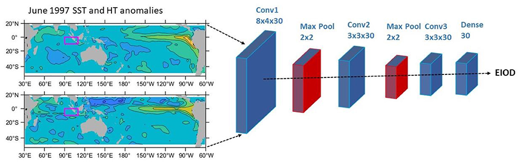
Figure 1. The structure of the CNN model. Input data domain is shown on the left as SST (upper) and heat content (lower) anomalies in the Indo-Pacific for an example month of June 1997. The focal region for the EIOD is shown by the magenta box (10°S-equator, 90–110°E). The first convolution layer of the CNN model is 8 × 4 with 30 filters, followed by a 2 × 2 maximum pooling layer; the second convolution layer is 3 × 3 with 30 filters, followed by a 2 × 2 maximum pooling layer; and the third convolution layer is also 3 × 3 with 30 filters, followed by a dense layer with 30 filters, before output to the monthly EIOD index.

A convolutional neural network (CNN) machine learning tool, trained with coupled ocean-atmosphere model outputs, has been applied in a predictability analysis of an ENSO index, achieving long-term prediction skills and overcoming the spring prediction barrier of the Pacific (Ham et al., 2019). Neural network machine learning techniques trained on observations and reanalysis products have also been applied in the prediction of positive IOD events (Ratnam et al., 2020). The Ratnam et al. model beat persistence forecasting for the starting months from February, though the winter forecast barrier was not evaluated and the predictability of the negative IOD was not a focus.

In this study, we adapt Ham et al. (2019) CNN model for a predictability study of the EIOD SST anomalies. The CNN model is trained using a selection of coupled climate models from Coupled Model Intercomparison Project Phases 5 and 6 (CMIP 5 and 6; Taylor et al., 2012; Eyring et al., 2016). We examine the model skills and assess predictions of both the strong positive and negative IOD events over recent decades. We also apply a gradient weighted class activation map (GRAD-CAM; Selvaraju et al., 2017) method to visualize the key features in the initial condition fields that generate the IOD predictions. The analysis can also assess the performance of the climate models in capturing the coupled ocean-atmosphere dynamics for the IOD events, as these models have been widely used to provide future projections of the IOD over the current century (e.g., Wang et al., 2017).

Methods

The machine learning model is adapted from a CNN model developed by Ham et al. (2019). CNN models comprise convolutional, pooling, and fully-connected types of layers and are primarily used in the field of pattern recognition within images (O'Shea and Nash, 2015). Their ability to encode image-specific features into the architecture at a reduced number of required model parameters [as compared to traditional Artificial Neural Networks (ANNs)] makes them more suitable for image-focused tasks. We use a training data domain in the tropical Indo-Pacific, 18°N-48°S, 30°E-300°E, and use a selection of CMIP class models (Taylor et al., 2012; Eyring et al., 2016). The climate model selection is based on an assessment of the ability of the CMIP5 coupled general circulation models in capturing the warming patterns associated with the Ningaloo Niño in the southeast Indian Ocean (Feng et al., 2013; Kataoka et al., 2014), as well as their ability to simulate the oceanic planetary wave propagation from the Pacific into the southeast Indian Ocean (Kido et al., 2016). The Ningaloo Niño and wave propagation criteria are to ensure that the CMIP models capture oceanic and atmospheric teleconnection between the tropical Pacific and the southeast Indian Ocean, which would ensure the Pacific influences on the Sumatra-Java upwelling system are captured in the models. Historical runs from 9 models were chosen from CMIP5 (CCSM4, CanESM2, CESM1-BGC, FGOALS-s2, GFDL-CM3, GFDL-ESM2G, GFDL-ESM2M, MRI-CGCM3, NorESM1-M); CMIP6 model selection matches the CMIP5 ensemble by selecting models from the same model centers, except that only 2 GFDL models from CMIP6 vs. 3 GFDL models from CMIP5 are used, so ACCESS-CM2 is used in the CMIP6 ensemble, while no ACCESS model was used in CMIP5 (for details of the CMIP models, see Taylor et al., 2012 and Eyring et al., 2016). The CNN model inputs include SST and upper 300 m ocean heat content (average temperature) anomalies from the CMIP models during 1861–2001, mapped onto a 2° × 2° grid (2,502 samples in total −139 sampling years from each model). CMIP data are detrended at each grid point before the CNN model training (the same detrending procedure is applied for the test data). The EIOD index, or the CNN model label, is defined as the average SST anomalies in the 10°S-equator, 90–110°E box, following Saji et al. (1999). The missing land cells are not included in the EIOD index calculation, whereas land cells are filled with zeros for the CNN model inputs.

As in Ham et al. (2019), we stack 3-monthly data for the CNN model input. We use monthly EIOD SST anomalies as the model labels, to train the CNN model at 1–13 lead months. Note that different CNN models are trained for different target months and lead months. 10 ensemble members are trained for each target month and lead month. There are three convolution layers in the CNN model, each with 30 filters, followed by max-pooling layers for the first two convolutions and a dense layer after the last one (Figure 1). Hyperbolic Tangent (Tanh) activation functions are used. Note we use a 3 by 3 filter for the last two convolutional layers. We use Python version 3.9.4 and Tensorflow on the CSIRO High-Performance Computing facility, supercomputer Bracewell for the CNN model training.

We use data from the National Centers for Environmental Prediction (NCEP) Global Ocean Data Analysis System during 1980–2020 (GODAS; Behringer and Yan, 2004) to evaluate the CNN model. GODAS product is based on a quasi-global configuration of the Geophysical Fluid Dynamics Laboratory Modular Ocean Model version 3, assimilating various ocean profile data. Similar to the CMIP model outputs, monthly GODAS upper ocean heat content and SST anomalies are fed into the CNN model to produce forecasts for the monthly EIOD index during 1982–2020 (averaged over the 10 ensemble members). We choose the 3 strongest positive IOD events (1994, 1997, 2019) and the 3 strongest negative IOD events (1998, 2010, and 2016) for further analysis.

The convolutional layers determine the output of neurons with the help of an activation function [that can be of linear or non-linear types e.g., binary step function, linear, sigmoid, tanh, ReLU, etc. (Sharma et al., 2017)]. The activation functions determine whether the input neurons should be activated and the summed weighted values with a bias should be transformed to produce an output. The sum of scalar products between weights is repeatedly adjusted through a process called backpropagation (Rumelhart et al., 1995). In other words, an activation function decides whether the neuron's input to the network is important in the process of prediction using the relevant mathematical operations. When the input data hits a convolution layer, it gets convolved with filters (formed by sets of weights or learnable kernels) to produce a 2D activation map. These activation maps can be visualized to see what characteristics are being picked up by the network to work toward final prediction results. An understanding of how deep learning models decide is very important for the deployment of robust, transparent, and trustworthy systems in real-world situations (Rio-Torto et al., 2020). Toward this end, most methods adopt a gradient-based approach and produce explanations called heatmaps by propagating pixel-wise relevance backward to the input of the network to highlight the most relevant pixels used for the final prediction results (Simonyan et al., 2013; Selvaraju et al., 2017; Sundararajan et al., 2017).

We use the gradient weighted class activation map (GRAD-CAM) method (Selvaraju et al., 2017), widely used in image classification problems without changing the CNN models, to analyze the activation in the last convolutional layer of the CNN model. We adapt the method in the application of a single label, y, with respect to its positive and negative extremities. We first calculate the gradient of the CNN model output against its final convolutional layer and then generate the activation maps by multiplying the averaged gradient and the last convolutional layer. That is, the weight for a particular filter or feature map k of the last convolutional layer of the CNN model is calculated as

$\begin{array}{l}{\alpha }_k=\frac{1}{Z}{\displaystyle \sum _{x,y,t}}\frac{\partial y}{\partial A_{x,y,t}^k}\end{array}$

where Z is the total number of spatial and temporal grid points, $\frac{\partial y}{\partial A^k}$ is the gradient of y with respect to a feature map A^k of the last convolutional layer, and then take the global pooling averaging over zonal, meridional, and time dimensions. The activation map is obtained by a linear combination of the weighted activation maps

$\begin{array}{l}{L}_{Grad-CAM}={\displaystyle \sum _k}{\alpha }_k{A}^k\end{array}$

In Selvaraju et al. (2017), they use a ReLU (Rectified Linear Unit) filter to retain positive values in the activation map, which they regard as having a positive influence on the classification. For our application, the predictand is the positive or negative extremities of the EIOD SST anomaly. Because of the non-linearity introduced by the convolution and filters, we need to retain both positive and negative values, assuming the regions with high absolute values in the activation maps contribute to the actual predictions. We normalize the activation map and only show absolute values >0.3. Regions with high absolute activation values are highlighted. Note that only the first member of the ensemble is used to generate the activation maps, which is essentially the same as using all 10 members.

Monthly persistence prediction of the SST anomalies is calculated using a covariance method following Torrence and Webster (1998). Furthermore, we use a set of hindcasts for monthly eastern IOD indices from a coupled model system, Australian Community Climate and Earth-System Simulator (ACCESS-S2), which is not included in the training data set of the CNN model, as an independent benchmark to compare with the skills from the CNN model. ACCESS-S2 is the Australian Bureau of Meteorology's multi-week to seasonal prediction system (Wedd et al., 2022), which became operational in October 2021. It is a major upgrade of ACCESS-S1 (Hudson et al., 2017) with a new ocean data assimilation system, which is based on a weakly-coupled ensemble optimal interpolation method (EnOI). ACCESS-S2 is based on the UK Met Office GloSea5-GC2 seasonal prediction system (MacLachlan et al., 2015). The atmosphere model of the ACCESS-S2 is resolved on a ~ 60 km horizontal resolution with 85 vertical levels, fully resolving the stratosphere. The ocean model of ACCESS-S2 is resolved at ~25 km horizontal resolution with 75 vertical levels. The atmosphere, land, ocean, and sea ice component models are coupled hourly by the Ocean Atmosphere Sea Ice Soil coupler version 3.0 (OASIS3, Valcke, 2013).

A 27-member time-lagged ensemble hindcast of ACCESS-S2 up to 8-month lead time for the period 1981–2018 is used to compare with the CNN model. The 27-member ensemble comprises three ensemble members on nine successive days (the 1st of the month and the eight prior days of the previous month). Therefore, the maximum lag time for the first forecast month (i.e., 1-month lead time) is 8 days. Monthly EIOD SST anomalies of the ACCESS-S2 are computed relative to the climatological mean (27-member ensemble mean for ACCESS-S2) from 1981 to 2018.

Results

In this section, we first present the CNN model skills and the predictions for the strongest IOD events; and then we analyze the activation maps of the CNN model predictions.

CNN model

The winter prediction barrier of the IOD is consistent with the persistence barrier in the eastern IOD SST anomalies, especially for persistence predictions starting from the October-January months (Figure 2A). On the other hand, the correlation scores for persistence predictions starting from March-July can reach about 0.6 at a 4-month lead. Essentially, the persistence prediction cannot overcome the boreal winter barrier, which is also the case for most coupled climate models (Luo et al., 2007; Zhao and Hendon, 2009; Doi et al., 2020).

FIGURE 2

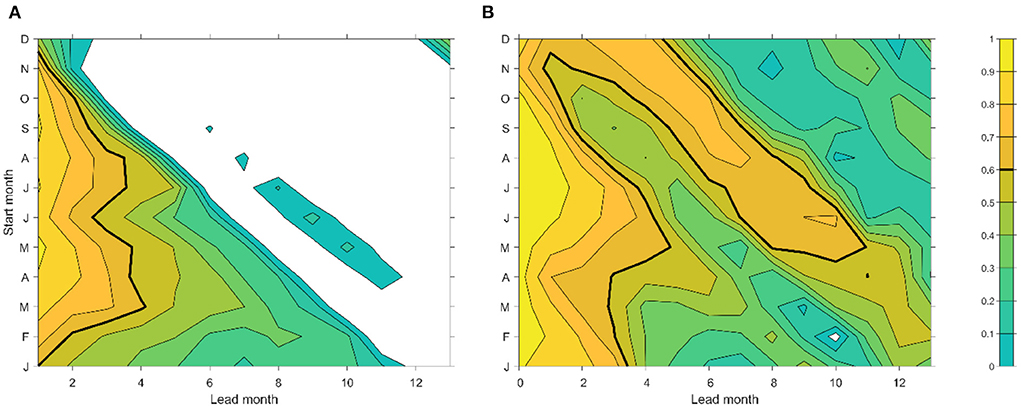
Figure 2. (A) Persistence of eastern IOD SST anomalies and (B) correlation prediction skills of the CNN model starting from each calendar month. Negative skills are not plotted and skills of 0.6 are denoted by bold contour lines. Persistence skills are calculated using GODAS data during the 1982–2020 period. In (B), the 1-month lead refers to the CNN model run using January to March input to predict April EIOD SST anomalies.

The CNN model trained by the CMIP models tends to beat persistence in most starting months and lead months and can improve the winter prediction barrier for predictions starting from the boreal autumn-winter months of November-January (Figure 2B). For the starting month of May, the 5-month lead prediction skill reaches 0.6. There is still a barrier to the prediction of SST anomalies around January, shown as a tongue of the low correlation of <0.6, extending from lead-3 for starting month of October to lead-12 for starting month of January. This barrier might be due to the low variance of the January SST variability in the eastern IOD region. There are greatly improved prediction skills for the March-May SST anomalies, shown as a high correlation (>0.6) tongue, from lead 3–5 months for a prediction starting in December to 8–10 month-lead for starting month of May, e.g. a prediction skill of almost 1-year lead.

The 2-month lead predictions for the eastern IOD SST anomalies achieve a linear correlation of 0.75 with the EIOD SST index from the GODAS reanalysis, capturing all the strong positive and negative IOD events during 1982–2020 (Figure 3A). The CNN model not only underpredicts the strong positive IOD events, e.g., 1994, 1997, and 2019, it also predicts reduced magnitude at the peaks of the weaker 2006–2008 IOD events. In comparison, the ACCESS-S2 predictions seem to capture most of the IOD peaks well, though only at short lead times (Supplementary Figure S4). The CNN model bias may be due to the coarse spatial resolution of the CMIP models used in the model training. Peaks of positive EIOD SST anomalies (negative IOD) appear to be better captured than the negative peaks (positive IOD).

FIGURE 3

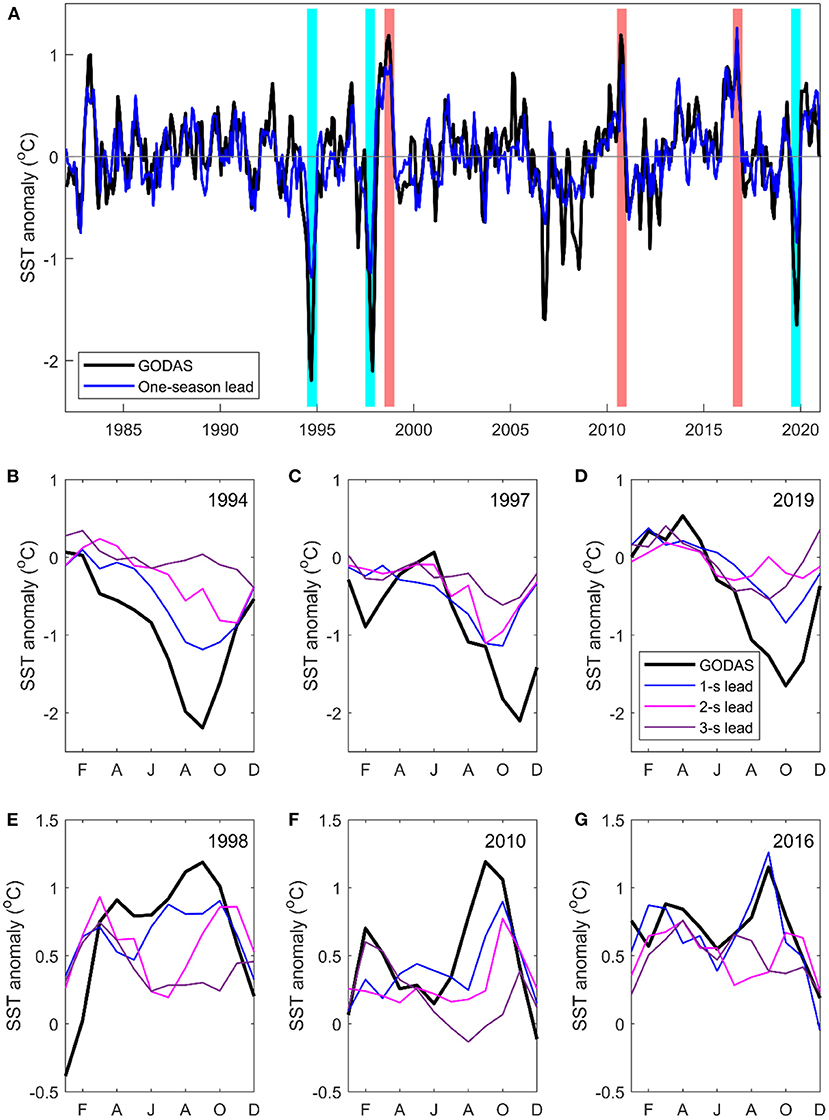
Figure 3. (A) Comparing the GODAS SST anomalies in the EIOD region with the 2-month lead predictions from the CNN model during 1982–2020. (B–G) The comparison between GODAS SST anomalies and the 2, 5, and 8-month lead (or 1, 2, and 3-season lead) CNN model predictions during three strong positive IOD events (negative SST anomalies) and three strong negative IOD events [cyan and light red color shadings in (A)]. The predictions are scaled by the standard deviations between GODAS SST anomalies and the zero-month lead CNN model prediction (a factor of 1.24).

The prediction skill of individual IOD events varies with different lead seasons (Figures 3B–G). Generally, the magnitude of the predicted values declines with increasing lead time, as in some dynamic model predictions (e.g., Zhao and Hendon, 2009). Despite the reducing magnitude, the peak 1994 positive IOD event can be predicted two seasons in advance. The CNN model forecast early peaks for the 1997 and 2019 IOD events for up to three-season leads, whereas the shorter lead-time forecasts capture the peak months better.

For the three strong negative IOD events, EIOD SST anomalies show positive peaks early in the year in February-April, before the main peaks in August-October. The main peaks of the SST anomalies are generally well-captured by the CNN model forecast at a one-season lead, with the long-lead forecasting generally having some delays in the peak phase. The SST peaks in February-April during the negative IOD events are to a certain extent captured by the CNN model up to three-season, which is consistent with the correlation forecast skills (Figure 2B). The February-April SST peak may be associated with the eastward propagating downwelling equatorial Kelvin waves, reflected from Rossby waves typically after a positive IOD event, transmitting warming signals to the Sumatra-Java coast (e.g., Feng and Meyers, 2003). Note that the eastward Yoshida-Wyrtki Jets in boreal fall tend to become weaker during a positive IOD event and have little change during an El Niño event (Chowdary and Gnanaseelan, 2007), so the eastward propagating signals are most likely due to planetary wave reflection at the western boundary of the Indian Ocean. Thus, the long lead prediction of EIOD SST variability in the late boreal winter-spring (February-April) season (Figure 2B), which overcomes the winter forecast barrier, is mostly derived from the prediction skills for the negative IOD events.

CNN model visualization

The standard deviations of the activation maps indicate regions that contribute the most to the CNN model forecast. For the forecast of September EIOD SST variability at one-season lead (May-June-July), the CNN model appears to be sensitive to the SST and/or upper ocean heat content anomalies in the equatorial eastern and central Pacific, tropical western Pacific, and tropical and southern subtropical Indian Ocean (Figure 4A). Note that the activation maps do not distinguish contributions from SST and heat content anomalies. For the CNN model to predict October EIOD SST anomalies using June-July-August inputs, the general patterns of the activation map standard deviations are quite similar (Figure 4B). The high sensitivity regions along the equatorial Pacific appear to shift southward, and eastward off the American coast. In the Indian Ocean, there is also high sensitivity off the west coast of Australia.

FIGURE 4

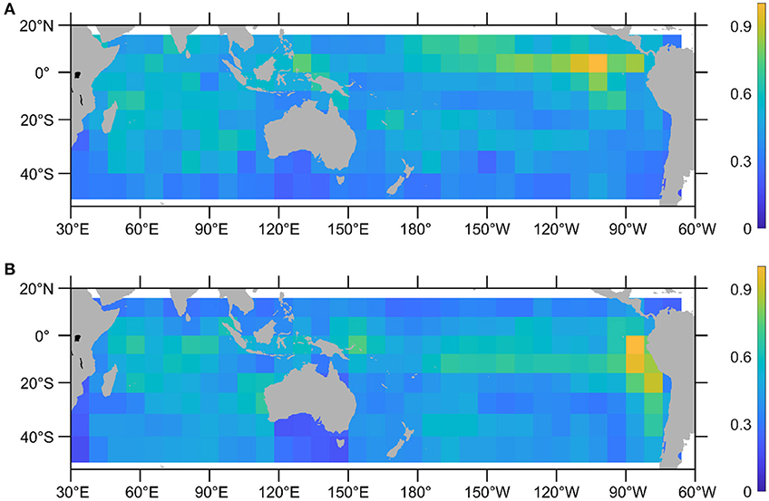
Figure 4. Standard deviations of the CNN model activation maps during 1982–2020: (A) using May-June-July inputs to forecast September EIOD SST anomalies, and (B) using June-July to August inputs to forecast October EIOD SST anomalies. The standard deviations are normalized with a maximum value of 1.

Individual events

The activation maps for the forecasts of individual strong positive (negative EIOD SST anomalies) and negative (positive EIOD SST anomalies) IOD events, similarly reveal locations that contribute to the individual predictions.

1994 positive IOD event

The activation map for the one-season lead forecast of the EIOD index in September 1994 shows contributions from regions in the far eastern equatorial Pacific, the east and southeast equatorial Indian Ocean, and the south Pacific centered around New Zealand (Figure 5). We overlay the SST and heat content anomalies in June 1994 and their differences between July and May 1994 to highlight the evolving features that may have contributed to the September 1994 EIOD index forecast.

FIGURE 5

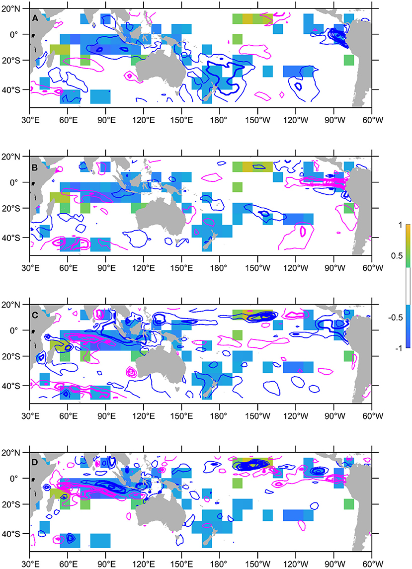
Figure 5. Activation map of using May-June-July SST and heat content anomalies to forecast the September 1994 EIOD peak (only showing absolute values >0.3). The activation map is overlaid with (A) SST anomalies in June 1994, (B) SST anomaly differences between July and May 1994, (C) heat content anomalies in June 1994, and (D) heat content anomaly differences between July and May 1994. Negative anomalies are denoted with blue contours and positive anomalies with magenta. Anomalies are plotted every 0.5°C, and the integer values are in bold contour. Zero contour lines are not plotted.

There could be a teleconnection from the far eastern Pacific into the Indian Ocean—although the SST was still colder than normal at that location (Figure 5A), there was a transition into a warm state (Figure 5B). However, it is more likely that the CNN model takes the cue from the eastern Indian Ocean to frame its forecast. The region was already colder than normal in June 1994 (Figure 5A), and there was a cooling tendency over the months (Figure 5B). There was a subsurface dipole structure in the heat content anomalies between the eastern and the central south equatorial Indian Ocean, denoting the equatorial upwelling Kelvin wave reaching the eastern boundary and wind-driven downwelling Rossby waves radiating from the eastern boundary (Figure 5C). There is also an indication that westward propagation of subsurface cold anomalies from the difference in heat content anomalies between July and May 1994 (Figure 5D). Rossby waves are closely linked to the southwest equatorial Indian Ocean warming during the IOD events (Li et al., 2002). The cold SST anomalies around New Zealand faded a bit with time and it is unlikely that they were a major source of predictability for the event.

The 1994 event has been regarded as an extreme IOD developed through the coupled ocean-atmospheric interaction in the Indian Ocean, anchored in the southeast Indian Ocean (Behera et al., 1999). The ability of the CNN model to take the cue of cooling early in the season for a full-strength IOD prediction suggests that the CMIP models can capture the coupled processes in the southeast tropical Indian Ocean (e.g., Liu et al., 2014) and the CNN model training process can translate the coupled dynamic inference into a statistical prediction.

1997 positive IOD event

For the 1997 positive IOD event, we examine the forecast of the October EIOD peak (Figure 3C). It has been generally recognized that the 1997 IOD was strongly influenced by the development of the extreme El Niño in the Pacific (Xie et al., 2002; Ashok et al., 2003). The EIOD index did not show any negative anomalies until July 1997 and quickly peaked in October-November (Figures 3C, 6), when the Pacific El Nino was in full development. During June-August, there were positive SST and heat content anomalies of >2°C in the equatorial eastern Pacific, with a significant increasing tendency (Figure 6). Significant warming and increase in ocean heat content were also present in the western Indian Ocean, signifying the teleconnection from the Pacific El Niño.

FIGURE 6

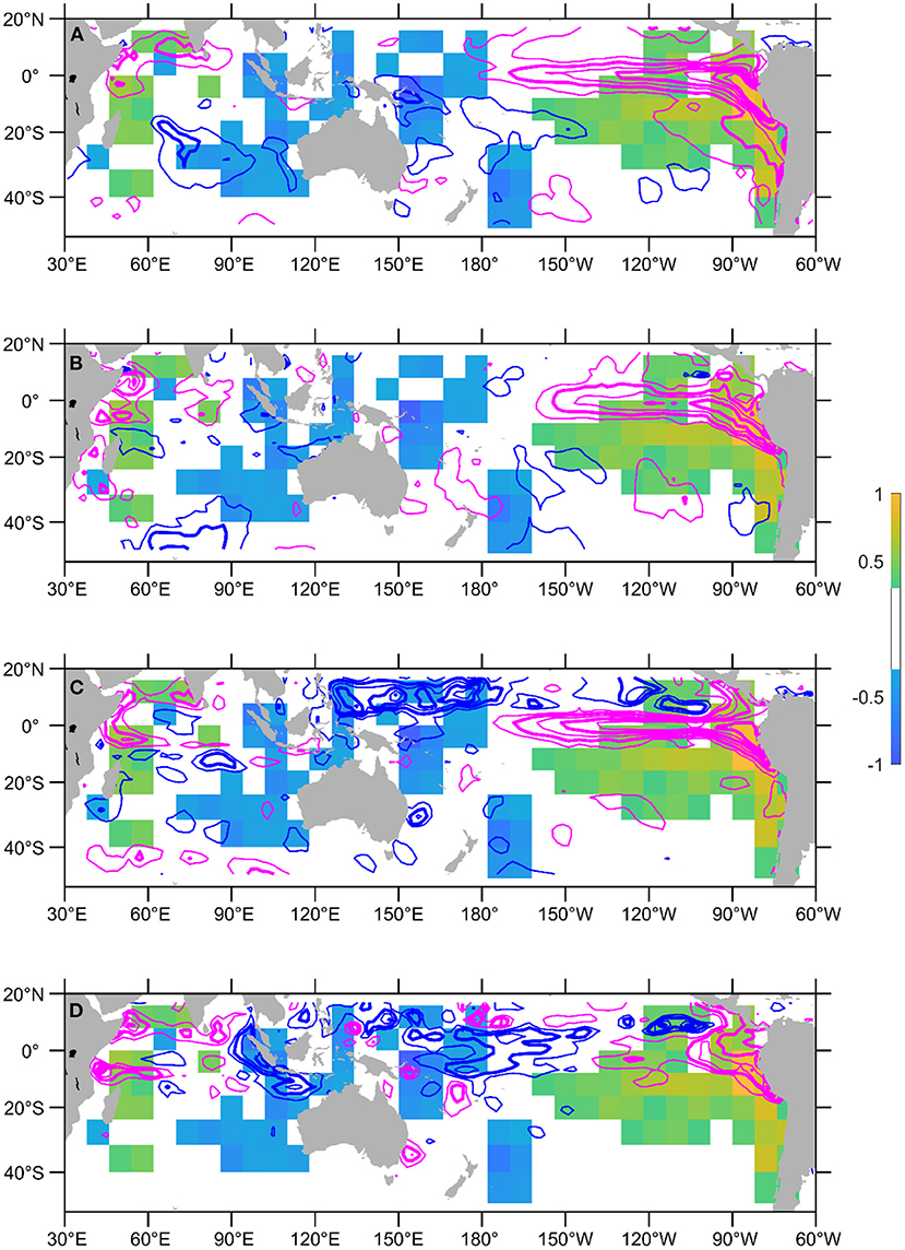
Figure 6. Activation map of using June-July-August SST and heat content anomalies to forecast the October 1997 EIOD peak (only showing absolute values >0.3). The activation map is overlaid with (A) SST anomalies in July 1997, (B) SST anomaly differences between August and June 1997, (C) heat content anomalies in July 1997, and (D) heat content anomaly differences between June and August 1997. Negative anomalies are denoted with blue contours and positive anomalies with magenta. Anomalies are plotted every 0.5°C, and the integer values are in bold contour. Zero contour lines are not plotted.

The activation map highlights that both the equatorial eastern Pacific and the western Indian Ocean regions may have contributed to the EIOD SST development in the following months in 1997, consistent with the El Niño trigger. The activation map also shows that the forecast has contributions from the western Pacific and the eastern IOD region. The cooling of the western Pacific warm pool might influence regional atmospheric circulation and facilitate coastal upwelling off Sumatra-Java (Annamalai et al., 2003). The lower upper ocean heat content in the western Pacific would also send shallow thermocline anomalies across the maritime continent and weaken the transport of the Indonesian throughflow (Wijffels and Meyers, 2004; Liu et al., 2015), which in turn would shoal the thermocline in the southeast tropical Indian Ocean and precondition the development of a positive IOD (e.g., Ummenhofer et al., 2017).

In the activation map, the significant patch in the southeast Indian Ocean may suggest a connection between the IOD and the Ningaloo Niño (e.g., Zhang et al., 2018) or the subtropical dipole (e.g., Behera and Yamagata, 2001), which needs some further attention.

2019 positive IOD event

The 2019 IOD is the most extreme positive IOD event over the past two decades, which is regarded as unique because the air-sea heat loss acted as key forcing for the EIOD cooling, instead of being a damping factor as in the previous events (Wang et al., 2020). The EIOD anomalies started to develop in June 2019 and reached peak value in October (Figure 3D). It is suggested that the anomalously high Australian High-pressure system and low sea level pressure anomalies in the South China Sea and the Philippines Sea drove cross-equatorial wind anomalies to initiate the air-sea feedback off the Sumatra-Java coast (Lu and Ren, 2020).

Although the CNN model doesn't use any atmospheric variables, the variations of the sea level pressure systems may have footprints in ocean temperatures. The one-season lead forecast for the October 2019 EIOD appears to be sensitive to the ocean temperature anomalies off the west coast of Australia, the Indonesian-Australian Basin, and the far western equatorial Pacific (Figure 7). In this longitude band, the cool SST anomalies in the south may be associated with the sea level pressure systems that set up the IOD mode as suggested by Lu and Ren (2020). Note that there was a multi-year cold spell off the west coast of Australia during 2016–2019 (Feng et al., 2021a), teleconnected from the west-central equatorial Pacific warming (Feng et al., 2021b). There was a weak central Pacific El Niño warming condition near the dateline being highlighted by the activation map, but its teleconnection to the equatorial western Indian Ocean appeared to be weak (Figures 7A,B). Despite the SST and heat content anomalies off the Sumatra-Java coast, they were only marginally detected by the activation map, which may be due to the different driving mechanisms of the 2019 IOD compared to the earlier events.

FIGURE 7

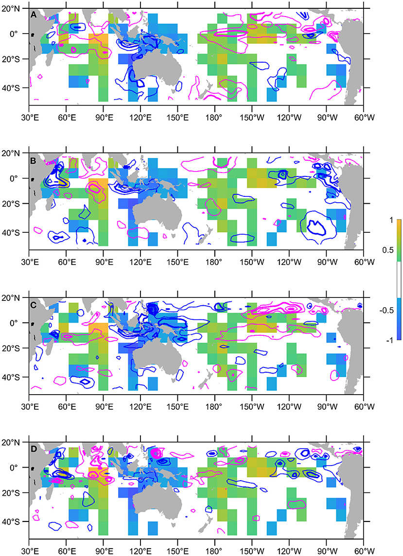
Figure 7. Activation map of using June-July-August SST and heat content anomalies to forecast the October 2019 EIOD peak (only showing absolute values >0.3). The activation map is overlaid with (A) SST anomalies in July 2019, (B) SST anomaly differences between August and June 1997, (C) heat content anomalies in July 2019, and (D) heat content anomaly differences between June and August 2019. Negative anomalies are denoted with blue contours and positive anomalies with magenta. Anomalies are plotted every 0.5°C, and the integer values are in bold contour. Zero contour lines are not plotted.

The long-lead prediction for the 2019 IOD event is also likely taking a cue from the interhemispheric temperature contrast (Supplementary Figure S1). It is not clear if this is related to the 2018–19 central Pacific El Niño mentioned in Doi et al. (2020), which had a weak teleconnection to the western Indian Ocean, however, it has been recently noted that the Ningaloo Niño region in the southeast Indian Ocean may have been acting as a bridge between the Pacific and Indian Ocean climate variability (Zhang and Han, 2018). The transmission of negative heat content anomalies from the western Pacific into the Indonesian-Australian Basin may also contribute (Supplementary Figures S1c,d).

Negative IOD events

All the three strong negative IOD events developed following strong canonical (1998 and 2016) or central Pacific (2010) El Nino events. SST anomalies in the eastern IOD region were already warm during the February-April period (Figure 3), which probably preconditioned the boreal autumn warming in the region. The reflection of downwelling Rossby waves into eastward propagating equatorial Kelvin waves may play a role to warm the equatorial eastern Indian Ocean (e.g., Feng and Meyers, 2003). The events may also be preconditioned by general warming across the Indian Ocean basin after an El Niño event (Yang et al., 2007), which is mostly due to the interplay between planetary wave propagations and local air-sea coupling in the Indian Ocean (Du et al., 2009).

Note that the ability of the CNN model to overcome the winter barrier is to some extent due to the long-lead prediction of the February-April SST anomalies in the eastern IOD pole (Figures 3E–G). The one-season lead predictions generally capture the phase and amplitude of the September peak well for these three events; however, the longer lead predictions tend to shift the peak amplitude to later months. Generally, the prediction skill at the three-season lead is low for the negative IOD peaks.

From the activation map of the 1998 negative IOD (Figure 8), the prediction of its September peak at one-season lead is influenced by the heat content and SST anomalies in both the equatorial Indian Ocean and equatorial eastern Pacific. In the tropical Indian Ocean, there was basin-wide warming in SST in June 1998, corresponding to the Indian Ocean Basin mode. In June 1998, there was a downwelling Rossby wave-like heat content anomaly pattern in the southwest tropical Indian Ocean which had reflected from the western boundary into equatorial Kelvin waves to reach the eastern boundary in July (Figures 8C,D).

FIGURE 8

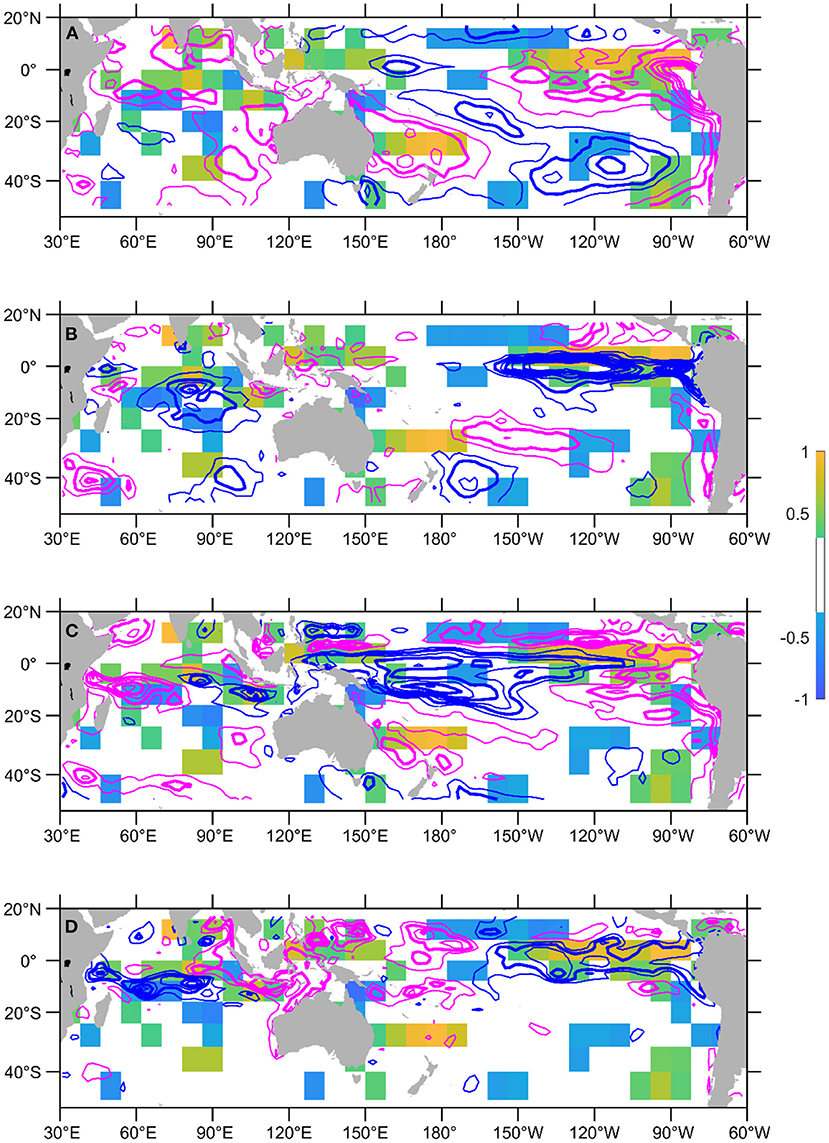
Figure 8. Activation map of using May-June-July SST and heat content anomalies to forecast the September 1998 EIOD peak (only showing absolute values >0.3). The activation map is overlaid with (A) SST anomalies in June 1998, (B) SST anomaly differences between July and May 1998, (C) heat content anomalies in June 1998, and (D) heat content anomaly differences between July and May 1998. Negative anomalies are denoted with blue contours and positive anomalies with magenta. Anomalies are plotted every 0.5°C, and the integer values are in bold contour. Zero contour lines are not plotted.

During the 2010 negative IOD, the prediction of the EIOD warming was most likely associated with the development of the 2010–11 strong La Nina event in the Pacific and its teleconnection into the Indian Ocean (Supplementary Figure S2). For the 2016 negative IOD, there was only a weak La Niña event developing in the Pacific, so the internal Indian Ocean processes such as the Rossby wave-Kelvin wave dynamics may play a larger role in contributing to the forecast (Supplementary Figure S3).

Comparison with the prediction skills of ACCESS-S2

Compared with the ACCESS-S2 model results, the CNN model skills appear to be on par with the dynamic forecasting model (Figure 9; Supplementary Figure S4). There is a good similarity between the prediction skills of the CNN model and ACCESS-S2 at different starting months, such as the reminiscence of the winter prediction barrier. ACCESS-S2 has better skills than the CNN model for predictions starting from July-September; however, the CNN model has better lead forecast skills than the ACCESS-S2 model for predictions starting from the March-June period, which is the critical season for the IOD development (Figure 9B). This is promising for a model trained only with CMIP simulations, suggesting that the CMIP models may have captured the key coupling mechanism to drive the IOD development. ACCESS-S2 also has slightly better skills for the starting month of January (Figure 9C).

FIGURE 9

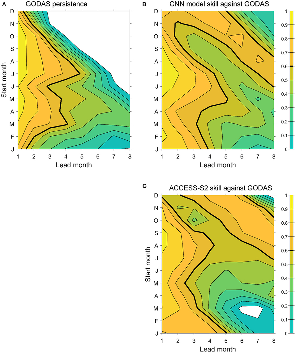
Figure 9. Intercomparison between the persistence and prediction skills for eastern IOD SST anomalies of the CNN model and ACCESS-S2: (A) persistence from GODAS, (B) correlation prediction skills of the CNN model, and (C) correlation prediction skills of ACCESS-S2. Negative skills are not plotted and skills of 0.6 are denoted by bold contour lines. The persistence and CNN model skill are interpolated to be consistent with the ACCESS-S2 lead time. See the correlation numbers in Supplementary Tables S1–3.

Discussion

In this study, we have applied a convolutional neural network (CNN) model to assess the predictability of the SST variability in the eastern pole of the IOD, off the Sumatra-Java coast in the tropical southeast Indian Ocean. The CNN model is trained using a selection of CMIP5 and CMIP6 model SST and upper ocean heat content anomalies in 3-monthly chunks. Results show that the CNN model can predict the EIOD SST variability at lead times of 1–2 seasons. The CNN model is also able to beat the persistence prediction and overcome the winter forecast barrier of the IOD. There is the potential for longer lead prediction of the EIOD for some events, such as the positive IOD of 2019 and the strong negative IOD events.

Visualization of the activation maps of the CNN model suggests that the model can respond to the different spatial contributions of remote and local forcing physics to generate skillful forecasts of both the positive and negative IOD events. The activation maps show that the one-season lead prediction of the 1994 positive IOD event mainly derives from internal Indian Ocean variability; the one-season lead prediction for the 1997 positive IOD is strongly influenced by the evolving El Niño in the Pacific; the prediction of the 2019 positive IOD has influences from cooling SST off the Australian coast. For the negative IOD events, the activation maps suggest that both the Indian Ocean Basin warming and downwelling Rossby and Kelvin waves are important contributions to the predictions. Evolving Pacific La Niña features also appear to be important for the negative IOD events. The wind anomalies in 1994 show a close coupling with upper ocean heat content anomalies (Supplementary Figure S5). The coupling in the other events is less obvious, though the reduction of upper ocean heat content during the 1997 event is associated with coastal upwelling driven by alongshore wind anomalies (Supplementary Figure S5).

In our approach, each CNN model is trained using thousands of realizations of the CMIP model outputs, similar to Ham et al. (2019). The ability of the CNN model to predict the EIOD SST variability suggests that the CMIP models capture the coupled dynamics in the Indo-Pacific to generate the IOD, both the internal Indian Ocean dynamics and the teleconnection between the Indian Ocean and the Pacific. The independency between the CMIP models and the GODAS reanalysis data also proves the robustness of the machine learning model. Still, the CNN model trained with the CMIP model outputs will inherit the model bias in CMIP models. CMIP models tend to simulate an easterly wind bias in the equatorial Indian Ocean with an overly shallow thermocline and large SST amplitude in the EIO region (Cai and Cowan, 2013), which may have caused the underrated positive EIOD SST anomalies. The observational records (including model reanalysis) are still rather short to train the CNN model architecture. Including the observational data thus cannot modify the model training in a significant way, consistent with Ham et al. (2019), as well as our test (not shown). In future studies, we may consider using isotherm depth anomalies, which may better represent upper ocean dynamics in the tropical oceans than the upper ocean heat content anomalies, in the CNN model training.

There are machine learning model architectures that only require short data records to train to achieve model stability and useful prediction skills. Taylor and Feng (2022) developed a fully convolutional network (U-Net), trained using a 70-year reanalysis product, to achieve reasonable multi-season prediction skills for the 2-dimensional monthly SST anomalies in the tropical-subtropical Pacific. A much simpler artificial neural network model based on correlations in the observational data can also achieve reasonable prediction skills for the IOD (Ratnam et al., 2020). Still, these models may not have desirable skills for rare climate events in the observational records or unseen events under a changing climate. Incorporating physical laws into the machine learning models may overcome the data deficiency (e.g., Raissi et al., 2019).

This paper has shown the potential of using CMIP model outputs to train a machine learning model to achieve skillful prediction of regional SST variability, as with the early success of applying the tool to the Pacific ENSO, a global climate mode. Whereas, the improved prediction of the cold events (positive IOD) in the eastern Indian Ocean may help drought and bushfire prediction in Australia and the Maritime Continent, the long lead prediction of the warm events (negative IOD) may help marine resource managers to mitigate the potential risks of the increased likelihood of marine heatwaves in the eastern Indian Ocean. The success may lead to prediction studies of regional SST variability and drivers in other parts of the world ocean and possibly implement this into a true forecast model.

Data availability statement

The original contributions presented in the study are included in the article/Supplementary material, further inquiries can be directed to the corresponding author/s.

Author contributions

MF conceived the idea, led the analysis, and drafted the manuscript. MA implemented the model visualization coding. All contributed to the analysis and commented on the manuscript. All authors contributed to the article and approved the submitted version.

Funding

This study was supported by a CSIRO-Chinese Academy of Sciences collaboration project and a CSIRO IM&T collaboration project. MF was also supported by the Centre for Southern Hemisphere Oceans Research (CSHOR), which was a joint initiative between the Qingdao National Laboratory for Marine Science and Technology (QNLM), CSIRO, University of New South Wales and University of Tasmania.

Acknowledgments

We thank Paul Branson from CSIRO to provide an internal review and four reviewers for helpful comments. CMIP data used in this study are from archives on Australian National Computational Infrastructure (https://nci.org.au). GODAS Reanalysis data are downloaded from Climate Prediction Center (https://www.cpc.ncep.noaa.gov/products/GODAS/).

Conflict of interest

Authors MF, FB, XZ, JH, and AH were employed by CSIRO Oceans and Atmosphere. Authors MA and BG were employed by CSIRO IM&T. Author LS was employed by Bureau of Meteorology.

The remaining authors declare that the research was conducted in the absence of any commercial or financial relationships that could be construed as a potential conflict of interest.

Publisher's note

All claims expressed in this article are solely those of the authors and do not necessarily represent those of their affiliated organizations, or those of the publisher, the editors and the reviewers. Any product that may be evaluated in this article, or claim that may be made by its manufacturer, is not guaranteed or endorsed by the publisher.

Supplementary material

The Supplementary Material for this article can be found online at: https://www.frontiersin.org/articles/10.3389/fclim.2022.925068/full#supplementary-material

References

Annamalai, H., Murtugudde, R., Potemra, J., Xie, S. P., Liu, P., and Wang, B. (2003). Coupled dynamics over the Indian Ocean: spring initiation of the zonal mode. Deep Sea Res. Part II Top. Stud. Oceanogr. 50, 2305–2330. doi: 10.1016/S0967-0645(03)00058-4

CrossRef Full Text | Google Scholar

Ashok, K., Guan, Z., and Yamagata, T. (2003). A look at the relationship between the ENSO and the Indian Ocean dipole. J. Meteorol. Soc. Jpn. Ser. II 81, 41–56. doi: 10.2151/jmsj.81.41

CrossRef Full Text | Google Scholar

Behera, S. K., Krishnan, R., and Yamagata, T. (1999). Unusual ocean-atmosphere conditions in the tropical Indian Ocean during 1994. Geophys. Res. Lett. 26, 3001–3004. doi: 10.1029/1999GL010434

CrossRef Full Text | Google Scholar

Behera, S. K., and Yamagata, T. (2001). Subtropical SST dipole events in the southern Indian Ocean. Geophys. Res. Lett., 28, 327–330, doi: 10.1029/2000GL011451

PubMed Abstract | CrossRef Full Text | Google Scholar

Behringer, D. W., and Yan, X. (2004). “Evaluation of the global ocean data assimilation system at NCEP: the Pacific Ocean. Eighth symposium on integrated observing and assimilation systems for atmosphere, oceans, and land surface,” in AMS 84th Annual Meeting (Seattle, WA: Washington State Convention and Trade Center), 11–15.

Google Scholar

Benthuysen, J. A., Oliver, E. C., Feng, M., and Marshall, A. G. (2018). Extreme marine warming across tropical Australia during austral summer 2015-2016. J. Geophys. Res. Oceans. 123, 1301–1326. doi: 10.1002/2017JC013326

CrossRef Full Text | Google Scholar

Cai, W., and Cowan, T. (2013). Why is the amplitude of the Indian Ocean Dipole overly large in CMIP3 and CMIP5 climate models?. Geophys. Res. Lett. 40, 1200–1205. doi: 10.1002/grl.50208

CrossRef Full Text | Google Scholar

Cai, W., Cowan, T., and Raupach, M. (2009a). Positive Indian Ocean dipole events precondition southeast Australia bushfires. Geophys. Res. Lett. 36, L19710. doi: 10.1029/2009GL039902

CrossRef Full Text | Google Scholar

Cai, W., Sullivan, A., and Cowan, T. (2009b). How rare are the 2006-2008 positive Indian Ocean Dipole events? An IPCC AR4 climate model perspective. Geophys. Res. Lett. 36, L08702. doi: 10.1029/2009GL037982

CrossRef Full Text | Google Scholar

Chowdary, J. S., and Gnanaseelan, C. (2007). Basin-wide warming of the Indian Ocean during El Niño and Indian Ocean dipole years. Int. J. Climatol. 27, 1421–1438. doi: 10.1002/joc.1482

CrossRef Full Text | Google Scholar

Doi, T., Behera, S. K., and Yamagata, T. (2020). Predictability of the super IOD event in 2019 and its link with El Niño Modoki. Geophys. Res. Lett. 47, e2019GL086713. doi: 10.1029/2019GL086713

CrossRef Full Text | Google Scholar

Doi, T., Storto, A., Behera, S. K., Navarra, A., and Yamagata, T. (2017). Improved prediction of the Indian Ocean Dipole Mode by use of subsurface ocean observations. J. Clim. 30, 7953–7970. doi: 10.1175/JCLI-D-16-0915.1

CrossRef Full Text | Google Scholar

Du, Y., Xie, S. P., Huang, G., and Hu, K. (2009). Role of air–sea interaction in the long persistence of El Niño–induced north Indian Ocean warming. J. Clim. 22, 2023–2038. doi: 10.1175/2008JCLI2590.1

CrossRef Full Text | Google Scholar

Eyring, V., Bony, S., Meehl, G. A., Senior, C. A., Stevens, B., Stouffer, R. J., et al. (2016). Overview of the Coupled Model Intercomparison Project Phase 6 (CMIP6) experimental design and organization. Geosci. Model Dev. 9, 1937–1958. doi: 10.5194/gmd-9-1937-2016

CrossRef Full Text | Google Scholar

Feng, M., Caputi, N., Chandrapavan, A., Chen, M., Hart, A., and Kangas, M. (2021a). Multi-year marine cold-spells off the west coast of Australia and effects on fisheries. J. Marine Syst. 214, 103473. doi: 10.1016/j.jmarsys.2020.103473

CrossRef Full Text | Google Scholar

Feng, M., McPhaden, M. J., Xie, S. P., and Hafner, J. (2013). La Niña forces unprecedented Leeuwin Current warming in 2011. Sci. Rep. 3, 1–9. doi: 10.1038/srep01277

PubMed Abstract | CrossRef Full Text | Google Scholar

Feng, M., and Meyers, G. (2003). Interannual variability in the tropical Indian Ocean: a two-year time-scale of Indian Ocean Dipole. Deep Sea Res. Part II Top. Stud. Oceanogr. 50, 2263–2284. doi: 10.1016/S0967-0645(03)00056-0

CrossRef Full Text | Google Scholar

Feng, M., Zhang, Y., Hendon, H. H., McPhaden, M. J., and Marshall, A. G. (2021b). Niño 4 West (Niño-4W) sea surface temperature variability. J. Geophys. Res. Oceans 126, e2021JC017591. doi: 10.1029/2021JC017591

CrossRef Full Text | Google Scholar

Feng, R., Duan, W., and Mu, M. (2014). The “winter predictability barrier” for IOD events and its error growth dynamics: results from a fully coupled GCM. J. Geophys. Res. Oceans 119, 2121–2128. doi: 10.1002/2014JC010473

CrossRef Full Text | Google Scholar

Ham, Y. G., Kim, J. H., and Luo, J. J. (2019). Deep learning for multi-year ENSO forecasts. Nature 573, 568–572. doi: 10.1038/s41586-019-1559-7

PubMed Abstract | CrossRef Full Text | Google Scholar

Holbrook, N. J., Scannell, H. A., Gupta, A. S., Benthuysen, J. A., Feng, M., Oliver, E. C., et al. (2019). A global assessment of marine heatwaves and their drivers. Nat. Commun. 10, 1–13. doi: 10.1038/s41467-019-10206-z

PubMed Abstract | CrossRef Full Text | Google Scholar

Hudson, D., Alves, O., Hendon, H. H., Lim, E., Liu, G., Luo, J.-J., et al. (2017). ACCESS-S1: the new Bureau of Meteorology multi-week to seasonal prediction system. J. Southern Hemisphere Earth Syst. Sci. 67, 3 132–159. doi: 10.1071/ES17009

CrossRef Full Text | Google Scholar

Kataoka, T., Tozuka, T., Behera, S., and Yamagata, T. (2014). On the Ningaloo Niño/Niña. Clim. Dyn. 43, 1463–1482. doi: 10.1007/s00382-013-1961-z

CrossRef Full Text | Google Scholar

Kido, S., Kataoka, T., and Tozuka, T. (2016). Ningaloo Niño simulated in the CMIP5 models. Clim. Dyn. 47, 1469–1484. doi: 10.1007/s00382-015-2913-6

CrossRef Full Text | Google Scholar

L'Heureux, M. L., Levine, A. F., Newman, M., Ganter, C., Luo, J. J., Tippett, M. K., et al. (2020). “ENSO prediction,” in El Niño Southern Oscillation in a Changing Climate, John Wiley & Sons, 227–246. doi: 10.1002/9781119548164.ch10

CrossRef Full Text | Google Scholar

Li, T., Zhang, Y., Lu, E., and Wang, D. (2002). Relative role of dynamic and thermodynamic processes in the development of the Indian Ocean dipole: an OGCM diagnosis. Geophys. Res. Lett. 29, 25–21. doi: 10.1029/2002GL015789

CrossRef Full Text | Google Scholar

Liu, L., Xie, S. P., Zheng, X. T., Li, T., Du, Y., Huang, G., et al. (2014). Indian Ocean variability in the CMIP5 multi-model ensemble: the zonal dipole mode. Clim. Dyn. 43, 1715–1730. doi: 10.1007/s00382-013-2000-9

CrossRef Full Text | Google Scholar

Liu, Q. Y., Feng, M., Wang, D., and Wijffels, S. (2015). Interannual variability of the Indonesian Throughflow transport: a revisit based on 30 year expendable bathythermograph data. J. Geophys. Res. Oceans 120, 8270–8282. doi: 10.1002/2015JC011351

CrossRef Full Text | Google Scholar

Lu, B., and Ren, H. L. (2020). What caused the extreme Indian Ocean Dipole event in 2019?. Geophys. Res. Lett. 47, e2020GL087768. doi: 10.1029/2020GL087768

PubMed Abstract | CrossRef Full Text | Google Scholar

Luo, J. J., Masson, S., Behera, S., and Yamagata, T. (2007). Experimental forecasts of the Indian Ocean dipole using a coupled OAGCM. J. Clim. 20, 2178–2190. doi: 10.1175/JCLI4132.1

CrossRef Full Text | Google Scholar

MacLachlan, C., Arribas, A., Peterson, K. A., et al. (2015). Global seasonal forecast system version 5 (GloSea5): a high-resolution seasonal forecast system. Q. J. R. Meteorol. Soc. 141, 1072–1084. doi: 10.1002/qj.2396

CrossRef Full Text | Google Scholar

Menard, F., Marsac, F., Bellier, E., and Cazelles, B. (2007). Climatic oscillations and tuna catch rates in the Indian Ocean: a wavelet approach to time series analysis. Fish. Oceanogr. 16, 95–104. doi: 10.1111/j.1365-2419.2006.00415.x

CrossRef Full Text | Google Scholar

O'Shea, K., and Nash, R. (2015). An introduction to convolutional neural networks. arXiv preprint arXiv:1511.08458.

Google Scholar

Raissi, M., Perdikaris, P., and Karniadakis, G. E. (2019). Physics-informed neural networks: a deep learning framework for solving forward and inverse problems involving nonlinear partial differential equations. J. Comput. Phys. 378, 686–707. doi: 10.1016/j.jcp.2018.10.045

CrossRef Full Text | Google Scholar

Ratnam, J. V., Dijkstra, H. A., and Behera, S. K. (2020). A machine learning based prediction system for the Indian Ocean Dipole. Sci. Rep. 10, 1–11. doi: 10.1038/s41598-019-57162-8

PubMed Abstract | CrossRef Full Text | Google Scholar

Rio-Torto, I., Fernandes, K., and Teixeira, L. F. (2020). Understanding the decisions of CNNs: an in-model approach. Pattern Recognit. Lett. 133, 373–380. doi: 10.1016/j.patrec.2020.04.004

CrossRef Full Text | Google Scholar

Rumelhart, D. E., Durbin, R., Golden, R., and Chauvin, Y. (1995). “Backpropagation: the basic theory,” in Backpropagation: Theory, Architectures and Applications, Psychology press, 1–34.

Google Scholar

Saji, N. H., Goswami, B. N., Vinayachandran, P. N., and Yamagata, T. (1999). A dipole mode in the tropical Indian Ocean. Nature. 401, 360–363. doi: 10.1038/43854

PubMed Abstract | CrossRef Full Text | Google Scholar

Selvaraju, R. R., Cogswell, M., Das, A., Vedantam, R., Parikh, D., and Batra, D. (2017). “Grad-cam: visual explanations from deep networks via gradient-based localization,” in Proceedings of the IEEE International Conference on Computer Vision, The Computer Vision Foundation, 618–626. doi: 10.1109/ICCV.2017.74

CrossRef Full Text | Google Scholar

Sharma, S., Sharma, S., and Athaiya, A. (2017). Activation functions in neural networks. Towards Data Sci. 6, 310–316. doi: 10.33564/IJEAST.2020.v04i12.054

CrossRef Full Text | Google Scholar

Shi, L., Hendon, H. H., Alves, O., Luo, J.-J., Balmaseda, M., and Anderson, D. (2012). How predictable is the Indian Ocean dipole? Mon. Weather Rev. 140:3867–3884. doi: 10.1175/MWR-D-12-00001.1

CrossRef Full Text | Google Scholar

Simonyan, K., Vedaldi, A., and Zisserman, A. (2013). Deep inside convolutional networks: visualising image classification models and saliency maps. arXiv preprint arXiv:1312.6034.

Google Scholar

Sundararajan, M., Taly, A., and Yan, Q. (2017). “Axiomatic attribution for deep networks,” in International Conference on Machine Learning, PMLR 70, 3319-3328.

Google Scholar

Taylor, J., and Feng, M. (2022). A deep learning model for forecasting global monthly mean sea surface temperature anomalies. arXiv preprint arXiv:2202.09967.

Google Scholar

Taylor, K.E., Stouffer, R. J., and Meehl, G. A. (2012). An overview of CMIP5 and the experiment design. Bull. Amer. Meteor. Soc. 93, 485–498. doi: 10.1175/BAMS-D-11-00094.1

PubMed Abstract | CrossRef Full Text | Google Scholar

Torrence, C., and Webster, P. J. (1998). The annual cycle of persistence in the El Nino/Southern Oscillation. Q. J. Meteorol. Soc. 24, 1985–2004. doi: 10.1256/smsqj.55009

PubMed Abstract | CrossRef Full Text | Google Scholar

Ummenhofer, C. C., Biastoch, A., and Böning, C. W. (2017). Multidecadal Indian Ocean variability linked to the Pacific and implications for preconditioning Indian Ocean dipole events. J. Clim. 30, 1739–1751. doi: 10.1175/JCLI-D-16-0200.1

CrossRef Full Text | Google Scholar

Ummenhofer, C. C., England, M. H., McIntosh, P. C., Meyers, G. A., Pook, M. J., Risbey, J. S., et al. (2009). What causes southeast Australia's worst droughts? Geophys. Res. Lett. 36, L04706. doi: 10.1029/2008GL036801

CrossRef Full Text | Google Scholar

Valcke, S. (2013). The OASIS3 coupler: a European climate modelling community software. Geosci. Model Dev. 6, 373–388. doi: 10.5194/gmd-6-373-2013

CrossRef Full Text | Google Scholar

Wang, G., Cai, W., and Santoso, A. (2017). Assessing the impact of model biases on the projected increase in frequency of extreme positive Indian Ocean dipole events. J. Clim. 30, 2757–2767. doi: 10.1175/JCLI-D-16-0509.1

CrossRef Full Text | Google Scholar

Wang, G., Cai, W., Yang, K., Santoso, A., and Yamagata, T. (2020). A unique feature of the 2019 extreme positive Indian Ocean Dipole event. Geophys. Res. Lett. 47, e2020GL088615. doi: 10.1029/2020GL088615

CrossRef Full Text | Google Scholar

Wedd, R. (2022). ACCESS-S2: the upgraded Bureau of Meteorology multi-week to seasonal prediction system. (To be submitted to the J. Southern Hemis. Earth Syst. Science).

Google Scholar

Wijffels, S., and Meyers, G. (2004). An intersection of oceanic waveguides: variability in the Indonesian Throughflow region. J. Phys. Oceanogr. 34, 1232–1253.doi: 10.1175/1520-0485(2004)034andlt;1232:AIOOWVandgt;2.0.CO;2

CrossRef Full Text | Google Scholar

Xie, S.-P., Annamalai, H., Schott, F. A., and McCreary, J. P. (2002). Structure and mechanism of south Indian Ocean climate variability. J. Climate.15, 864–878. doi: 10.1175/1520-0442(2002)015andlt;0864:SAMOSIandgt;2.0.CO;2

CrossRef Full Text | Google Scholar

Yang, J., Liu, Q., Xie, S. P., Liu, Z., and Wu, L. (2007). Impact of the Indian Ocean SST basin mode on the Asian summer monsoon. Geophys. Res. Lett. 34, L02708. doi: 10.1029/2006GL028571

CrossRef Full Text | Google Scholar

Yang, Y., Xie, S. P., Wu, L., Kosaka, Y., Lau, N. C., and Vecchi, G. A. (2015). Seasonality and predictability of the Indian Ocean dipole mode: ENSO forcing and internal variability. J. Clim. 28, 8021–8036. doi: 10.1175/JCLI-D-15-0078.1

CrossRef Full Text | Google Scholar

Zhang, L., and Han, W. (2018). Impact of Ningaloo Niño on tropical Pacific and an interbasin coupling mechanism. Geophys. Res. Lett. 45, 11–300. doi: 10.1029/2018GL078579

CrossRef Full Text | Google Scholar

Zhang, L., Han, W., Li, Y., and Shinoda, T. (2018). Mechanisms for generation and development of the Ningaloo Niño. J. Clim. 31, 9239–9259. doi: 10.1175/JCLI-D-18-0175.1

CrossRef Full Text | Google Scholar

Zhao, M., and Hendon, H. H. (2009). Representation and prediction of the Indian Ocean dipole in the POAMA seasonal forecast model. Q. J. R. Meteorol. Soc. 135, 337–352. doi: 10.1002/qj.370

CrossRef Full Text | Google Scholar