Assessment of CMIP6 models' performance in simulating present-day climate in Brazil

Introduction

According to the Sixth Assessment Report (AR6) of the Intergovernmental Panel on Climate Change (IPCC), climate system warming is already evident, and the global surface temperature change has been ~1.1°C from 1850 to 1900, very likely due to human influence (IPCC, 2021). Global warming changes the water cycle (Held and Soden, 2006; Alfieri et al., 2017) and modifies the frequency and intensity of extreme events. It is already affecting every region on Earth, leading to significant risks to ecosystems and diverse sectors of society (Sillmann et al., 2013; Chadwick et al., 2014; Wang et al., 2014; Fischer and Knutti, 2016; Oppenheimer et al., 2019; Cook et al., 2020; Ashfaq et al., 2021; Masson-Delmotte et al., 2021). In addition, climate projections suggest that the probability of extreme climatic events will continue to increase over the 21st century (IPCC, 2021). Therefore, it is essential to investigate how these changes will affect society's resilience and to provide helpful information for enhancing climate change risk management and enabling informed decision-making. Such changes in human society and ecosystems vary among different regions and seasons (IPCC, 2021).

General circulation models (GCMs) are the main tools to approach these issues. This is done by analyzing the simulations of different GCMs for future scenarios and investigating the climate system response to the changes in radiative forcing (Taylor et al., 2012; Flato et al., 2013). Climate models are widely applied to project future climate change at global and regional scales (Su et al., 2013; Bannister et al., 2017; Gusain et al., 2020), thus their performance in simulating the present-day and past climates need to be evaluated. Overall, the models present different levels of skill in simulating specific variables over an area of interest, so a model-by-model analysis is necessary (Srivastava et al., 2020). In addition, it is necessary to assess model uncertainty through a comparison of historical simulations against observations, using a broad range of measurements to determine whether these models properly simulate the main climatological patterns of a region. Therefore, understanding the present-day and past climate at local scales is essential for more effective risk management under future climate change.

Most recent, simulations from state-of-the-art versions of GCMs have become available through the Coupled Model Intercomparison Project Phase 6 (CMIP6), with a substantial increase in the number and scope of experiments (Eyring et al., 2016; O'Neill et al., 2016). These simulations provide a new opportunity to evaluate the Earth system response to change in radiative forcings during the 21st century. CMIP6 models have typically updated versions of the models that participated in previous phases of CMIP. This new set of models has improved spatial resolution, physical parameterizations (i.e., cloud microphysics), and better representations of various earth system processes (such as biogeochemical cycles) and components (such as ice sheets) (Eyring et al., 2016; Stouffer et al., 2017).

The evaluation of CMIP6 simulations over several regions suggests that model output exhibits differences from earlier CMIP phases (Almazroui et al., 2020a,b, 2021a,b; Ortega et al., 2021). Some studies evaluated CMIP6 GCMs historical runs over several parts of the globe, including South America (SA) and Brazil. In a preliminary analysis, Rivera and Arnould (2020) evaluated the performance of CMIP6 over Southwestern SA using its long-term historical runs. They listed the subset of models that best represent the precipitation variability in this region. Fan et al. (2020) noted that most CMIP6 models reproduced the spatial pattern of climatological annual mean temperature over the global land surface properly, but with large variability across models and regions. Furthermore, CMIP6 could capture the sign of trends of mean global surface temperatures shown by the observational data during the periods 1901–1940 (warming), 1941–1970 (cooling), and 1971–2014 (rapid warming), despite showing less spatial variability compared with the observations. Assessing large ensembles of some CMIP6 models, Díaz et al. (2021) found that most models have limitations in correctly reproducing the precipitation characteristics of the South American Monsoon. Ortega et al. (2021) evaluated the historical simulations of precipitation and temperature from CMIP5 and CMIP6 models over some regions in Central and South America (CSA). They identified a subset of CMIP6 models that best represent the present-day climate in these regions. Additionally, they found that the ensemble mean of the CMIP6 models shows performance similar to the best CMIP5 models regarding precipitation, and also that it better simulated the height-temperature variation over the Andes compared to CMIP5.

Due to vast social and environmental vulnerabilities, besides an agricultural-based economy, Brazil (and SA) frequently suffers negative impacts caused by current climate variability and extreme climate events and could be highly affected by the projected future climate change (Baettig et al., 2007; Meehl et al., 2007; Torres et al., 2012; Torres and Marengo, 2013; Masson-Delmotte et al., 2021). In a recent study, Shimizu et al. (2022) used a multi-model analysis with the Detection and Attribution experiments from CMIP6 to better understand the physical processes related to precipitation trends over North and Northeast Brazil, but no assessment of historical runs was presented. Pereima et al. (2022) compared different CMIP5 and CMIP6 ensemble performances in simulating precipitation in Southern Brazil. Despite the detailed analyses, this study does not provide a comparison among the models, besides being limited to one region and for precipitation only. Thus, there is still a lack of studies that points out the best CMIP6 models to simulate the main climatic features of Brazil. In addition, the evaluation of sub-regional scale performance is also lacking, which is of concern because most of these models are widely used for statistical and dynamical downscaling and impact studies.

Therefore, this paper aims to assess the performance of CMIP6 models in reproducing the historical climate over Brazil. The objective was to answer the following questions: How well do the CMIP6 models simulate the main spatial patterns of precipitation, temperature, and circulation over Brazil? Does the CMIP6 ensemble mean reproduce the frequency distributions of temperature and precipitation similar to the observations? Which models best simulate the annual cycles and seasonal means of temperature and precipitation in some key regions of Brazil?

Data and methods

Global climate model data

The Brazilian climate was examined using the Coupled Model Intercomparison Project Phase 6 (CMIP6) models (Eyring et al., 2016). We used historical simulations of monthly mean surface air temperature, precipitation, and zonal and meridional winds (200 and 850 hPa) from 35 GCMs obtained from the CMIP6 archives (https://esgf-node.llnl.gov/search/cmip6/). A list of CMIP6 models, their countries, and their horizontal resolution are shown in Table 1. Only one ensemble member from each model is considered in the analyses. For all the models, we used the r1i1p1f1 member, except for the HadGEM3 family, where the r1i1p1f3 member was chosen due to a lack of f1 simulations.

TABLE 1

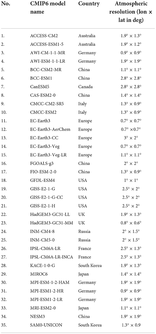
Table 1. List of CMIP6 historical global climate models used in this study.

Although the CMIP6 historical runs cover the period of 1850–2014, in this paper, we analyze historical simulations over the period 1995–2014 (also called present-day), as established by AR6 Working Group I (Masson-Delmotte et al., 2021) and used by Almazroui et al. (2021a), Llopart et al. (2021), Lv et al. (2021) and Ortega et al. (2021). To facilitate intercomparison, all the GCM outputs were interpolated onto a common grid of 1° × 1° resolution by the bilinear interpolation method.

Observation-based dataset

The reference observation datasets used in this study were as follows: (i) monthly precipitation and temperature compiled by the Climatic Research Unit (CRU) Time Series of the University of East Anglia version 4.03 (Harris et al., 2014, 2020). The CRU dataset is derived from an analysis of over a thousand individual meteorological station records and covers the period of 1901–2018 at 0.5° × 0.5° spatial resolution These time series have been subjected to extensive quality assessments in previous studies that showed that CRU data reproduce precipitation and temperature adequately over SA (Fan et al., 2020; Rivera and Arnould, 2020; Almazroui et al., 2021a), and (ii) monthly averaged winds at 850hPa and 200hPa from European Reanalysis 5 (ERA5) (Olauson, 2018; Hersbach et al., 2020) on a 0.5-resolution global grid spanning the period from 1995 to 2014. ERA5 is the most recent reanalysis dataset from ECMWF and is commonly used in model assessment studies (Luo et al., 2020; Ortega et al., 2021). The observational dataset was interpolated onto model grids as described in Section Global climate model data.

Methods

To assess the ability of CMIP6 models to simulate the main climatic characteristics over Brazil, first, we analyzed the large-scale circulation patterns at two different vertical levels (850 and 200 hPa) and biases of GCMs-simulated seasonal (austral summer and winter) mean precipitation and surface temperature relative to observations (model minus observation). Second, we assessed the skill of the models at simulating seasonal variability in some key regions of Brazil using probability density functions (PDFs) and the annual cycle of monthly precipitation and surface mean temperatures. The five key regions of Brazil are the Northern Amazon (NAZ), Southern Amazon (SAZ), South America Monsoon region (SAM), Northeast Brazil (NEB), and La Plata Basin (LPB) as suggested by Alves et al. (2021) (shown in Figure 1). These regions were chosen because they each exhibit a well-defined seasonal precipitation cycle and represent sub-continental regions of broadly climatic coherency in all the domains, being relevant to the studies of the Brazilian biomes, climatic, hydrological, and social systems. They also are important to several socioeconomic sectors, such as water, energy, and agriculture. The NAZ and SAZ regions are characterized by a high total amount of precipitation (2,500 to 3,000 mm/year) and high temperatures (annual averages between 26 and 28°C) compared to other Brazilian regions (Marengo and Nobre, 2009). The rainy season in the southern portion of the Amazon Region occurs during December–January–February, associated with the Chaco Low and the South Atlantic Convergence Zone (SACZ). In the northern part, the rains are heavier from April to May, related to the Inter-Tropical Convergence Zone (ITCZ) position (Marengo and Nobre, 2009). The NEB region also presents high average temperatures (an average of 26.5°C in summer and 24.5°C in winter), but it rains less than the other regions. Despite that, NEB has a well-defined rainy season that occurs during March–April–May (due to the ITCZ position) with an average seasonal precipitation of about 400 mm. In these three regions, the prevailing winds are the trade winds that have annual and inter-annual variability (Marengo et al., 2004). The SAM region has a well-defined rainy season, with an average rainfall of 776 mm in summer and 34 mm in winter. In summer, the South America Low-Level Jet (SALLJ) transports moisture from the Amazon to this region (Vera et al., 2006). The NEB region also presents seasonal temperature variability due to the position of the high-level jet. It is possible to have the arrival of cold fronts, reducing the temperature in the region (Andrade and Cavalcanti, 2004). The LPB region has an even more significant seasonal variability in temperature, with an average temperature of 25°C in summer and 16.5°C in winter. This region, however, has a well-defined rainy season in its northern part and not very defined in its southern half, with rainfall well distributed throughout the year. Hence, the average rainfall varies from 496 mm in the summer to 215 mm in the winter. The prevailing winds are due to the positioning of the subtropical high (Reboita et al., 2019), in addition to the variations due to transients, frequent in the region (cold fronts, cyclones, CCMS, etc.) (Velasco and Fritsch, 1987; Andrade and Cavalcanti, 2004).

FIGURE 1

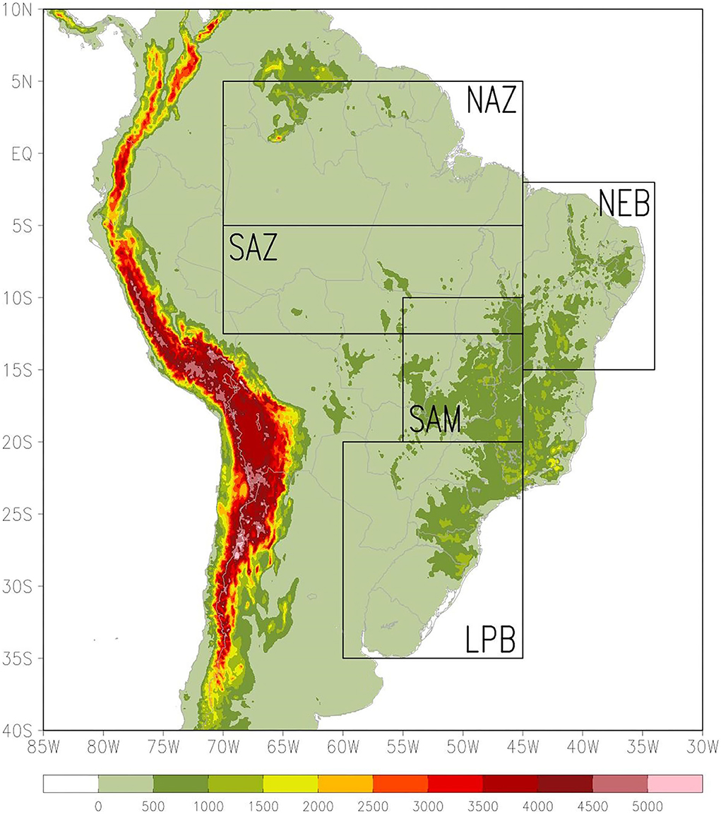
Figure 1. Topography of the study area (m; shaded) with the sub-regions delimited: Northern Amazon (NAZ; 5°S−5°N, 70°-45°W), Southern Amazon (SAZ; 12,5°-5°S, 70°-45°W), Northeast Brazil (NEB; 15°-12°S, 45°-34W), South America Monsoon (SAM; 20°-10°S, 55°-45°W) and La Plata Basin (LPB; 35°-20°S, 65°-45°W).

Finally, we calculated statistical metrics comparing each grid point of models and observations, to assess the models' ability to simulate the rainfall and temperature spatial variability. The metrics used were as follows: Pearson's correlation coefficients (R), standard deviations (SD), and root-mean-square errors (RMSE) presented seasonally through Taylor diagrams (Taylor, 2001).

Results

Recognizing the spatial patterns

This section analyzes the austral summer (December, January, and February—DJF) and austral winter (June, July, and August—JJA) atmospheric circulation patterns and temperature and precipitation biases. All analyses were made for the climatological period spanning from 1995 to 2014.

Circulation patterns

The analysis of atmospheric circulation patterns is widely used to infer models' ability to reproduce primary climate patterns that are related to other variables such as temperature and precipitation. Figure 2 shows the ERA5, the multi-model ensemble mean, and each CMIP6 model's (refer to Table 1) climatological circulation at 850 hPa during December, January, and February (DJF). Shading represents the magnitude of the winds (above 5 ms⁻¹).

FIGURE 2

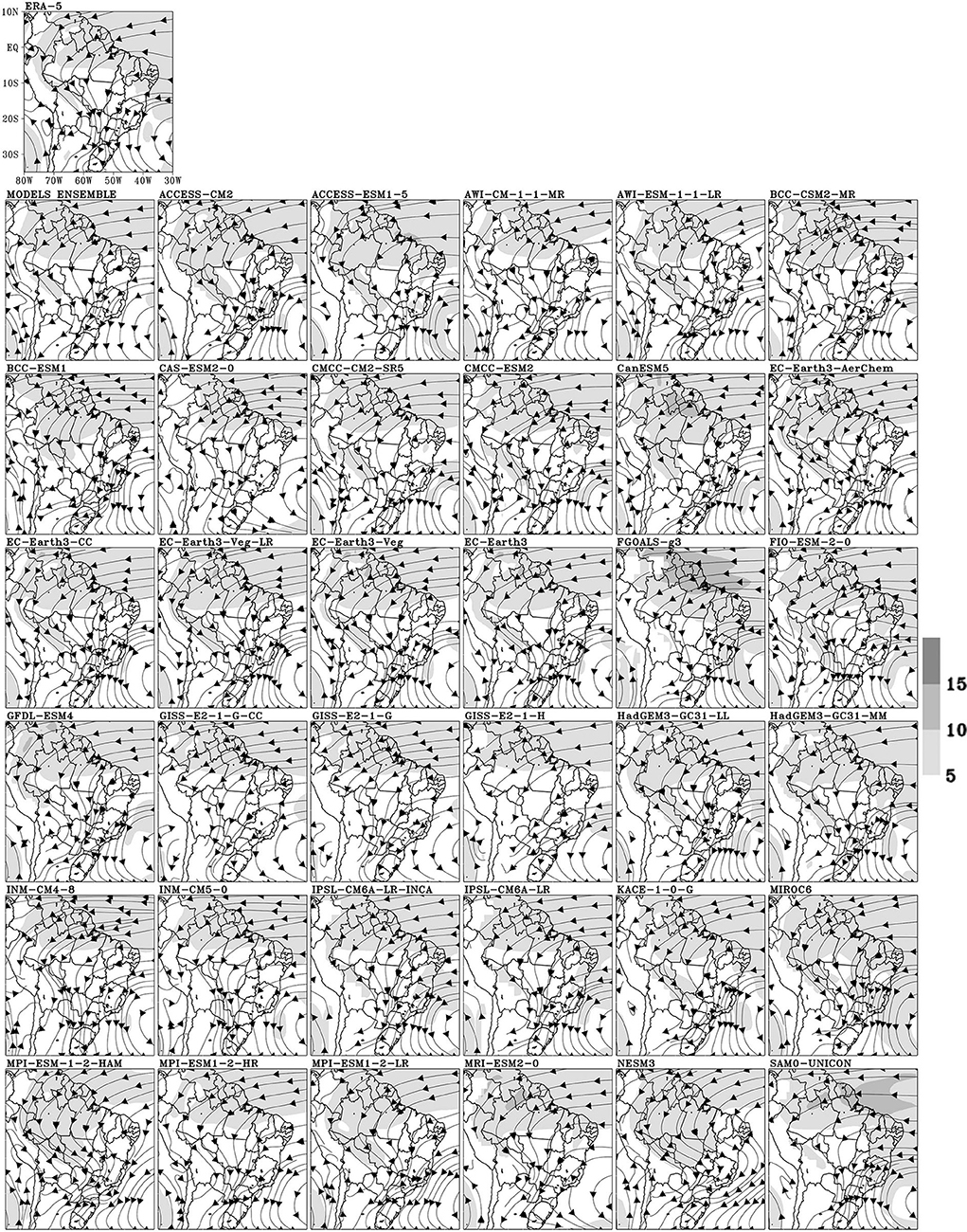
Figure 2. Streamlines and magnitude of climatological winds (m/s) at 850 hPa simulated by the multi-model ensemble mean, individual CMIP6 models, and ERA-5 reanalysis (top left) for austral summer (DJF) during the historical period. The shaded regions represent wind magnitude starting from 5 m/s while the vector shows the wind direction.

ERA5 climatological circulation (top left panel) shows the widely known low-level austral summer circulation pattern (Zhou and Lau, 1998; Vera et al., 2006) with the trade winds entering SA through the east coast of the Amazon rainforest. This flow, known as the South American Low-Level Jet (SALLJ), carries the moisture from the Atlantic Ocean to the Amazon Basin and turns north-northwesterly below 10°S due to the presence of the Andes (Marengo et al., 2004). This is an important feature for maintaining the South American Monsoon System (Vera et al., 2006) since the north-northwesterly circulation is responsible for transporting moisture and heat from the tropical to the subtropical regions of SA. Furthermore, the circulation pattern over the east coast of Brazil is influenced by the western edge of the South Atlantic Subtropical High (SASH).

In general, most CMIP6 models were able to simulate the major features of the austral summer low-level circulation. However, it is noted that models tend to weaken the trade winds compared to ERA5 near the east of Northeast Brazil. This deficiency is not present in FGOALS-g3, FIO-ESM-2-0, HadGEM3-GC31-LL, HadGEM3-GC31-MM, IPSL-CM6A-LR-INCA, IPSL-CM6A-LR, KACE-1-0-G, MIROC6, and SAM0-UNICON models. In addition, AWI-ESM-1-1-LR, MPI-ESM-1-2-LR, MPI-ESM-1-2-HAM, and NESM3 models display easterly trade winds with a more intense meridional (southerly) flow than ERA5 over the equator. Representing the intensity and orientation of trade winds in this region is important for the placement of the Intertropical Convergence Zone (ITCZ). Concerning the north-northwesterly low-level circulation below 10°S in the interior of SA, some models simulate a more intense westerly component (e.g., ACCESS-CM2, BCC-ESM1-5, CanESM5, GFDL-ESM4, KACE-1-0-G, MPI-ESM1-2-LR, MPI-ESM1-2-HAM, and NESM3), thus resulting in an increased low-level convergence over the Southeast and Central Brazil regions, given the interaction between this flow and the circulation originating from the SASH. These differences simulated by the GCMs suggest that the transport of moisture and heat from the tropical to the subtropical regions is reduced compared to observations, which is particularly important for maintaining the South American Monsoon System (Vera et al., 2006). GISS family models present a northeasterly flow over the interior of SA, which is not seen in ERA5. The western edge of the SASH over the east coast of Brazil is well represented by most of the CMIP6 models, except for NESM3. The SASH location is shifted westward in the NESM3 model.

During the austral winter (JJA) (Figure 3), trade winds in the tropical region of Brazil have a southerly component. Furthermore, winds are stronger over this region than during the austral summer (DJF). The SASH is closer to the east coast of SA when compared to the austral summer, inducing a northerly wind component south of 15°S over the continent. Overall, CMIP6 models reproduce the general atmospheric circulation better for JJA than for DJF at 850 hPa.

FIGURE 3

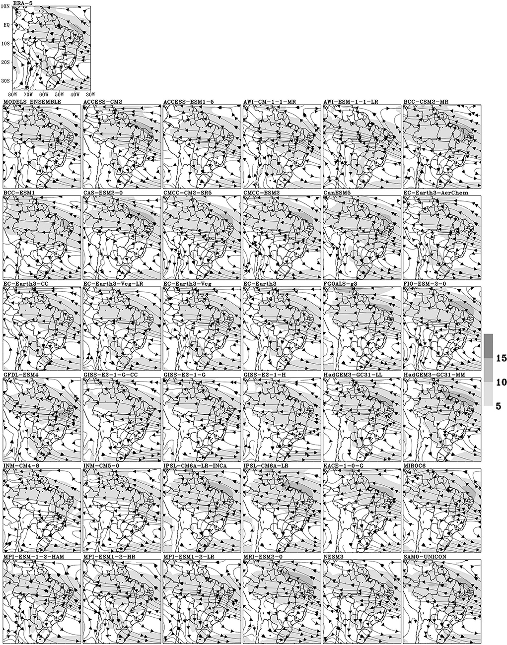
Figure 3. Streamlines and magnitude of climatological winds (m/s) at 850 hPa simulated by the multi-model ensemble mean, individual CMIP6 models, and ERA-5 reanalysis (top left) for austral winter (JJA) during the historical period. The shaded regions represent wind magnitude starting from 5 m/s while the vector shows the wind direction.

Patterns of upper-level wind circulation at 200 hPa during austral summer (DJF) are shown in Figure 4. ERA5 (top left panel) shows an undulating flow formed by an anti-cyclone centered over Bolivia, which is known as the Bolivian High, and a trough over northeast Brazil and the tropical South Atlantic Ocean (Virji, 1981). The undulating flow responds to mid-tropospheric heating by latent heat release that occurs mainly in the Amazon basin (Lenters and Cook, 1997). The Bolivian High has a near-symmetrical structure in meridional and zonal directions. The trough has a northwest-southeast orientation over the Atlantic Ocean and northeast Brazil. The northern branch of the subtropical jet can be seen between 30°S and 35°S. It is noted that BCC-CSM2-MR, FIO-ESM-2-0, HadGEM3-GC31-LL, HadGEM3-GC31-MM, SAM0-UNICON, and the multi-model ensemble-mean reproduce well the main climatological features of the austral summer upper-level circulation. However, some models, such as CAS-ESM2-0 and FGOALS-g3, show some important differences compared to ERA5. They have limitations in reproducing key features such as the Bolivian High, the trough over northeast Brazil and, the subtropical jet circulation patterns that are critical in determining the precipitation in parts of Brazil. AWI-ESM-1-1-LR, BCC-ESM1, EC-Earth3 family, INM-CM4-8, INM-CM5-0, KACE-1-0-G, MPI-ESM-1-2-HAM, and NESM3 do not represent the near-symmetrical structure of the Bolivian High. In addition, the Bolivian High is shifted equatorward in GISS-E2-1-G-CC, GISS-E2-1-G, MPI-ESM1-2-HR, and MRI-ESM2-0 models, while it is shifted westward in CanESM5, GISS-E2-1-H, INM-CM4-8, and INM-CM5-0. Another limitation presented by the GISS family and NESM3 models concerns the absence of the trough over northeast Brazil and the tropical South Atlantic Ocean. Moreover, AWI-ESM-1-1-LR, BCC-ESM1, EC-Earth3family, and MPI family show the trough with a west-east orientation, different from what is observed in ERA5. The subtropical jet is equatorward (poleward) of its real position in the ACCESS-CM2, ACCESS-CM1-5, AWI-CM-1-1-MR, BCC-ESM1, CAS-ESM2-0, CanESM5, FGOALS-g3, GFDL-ESM4, IPSL-CM6A-LR, IPSL-CM6A-LR-INCA, KACE-1-0-G, MIROC6, and MRI-ESM2-0 (EC-Earth3-CC, EC-Earth3-Veg-LR, EC-Earth3, INM-CM4-8, INM-CM5-0, MPI-ESM-1-2-HAM, and NESM3) models.

FIGURE 4

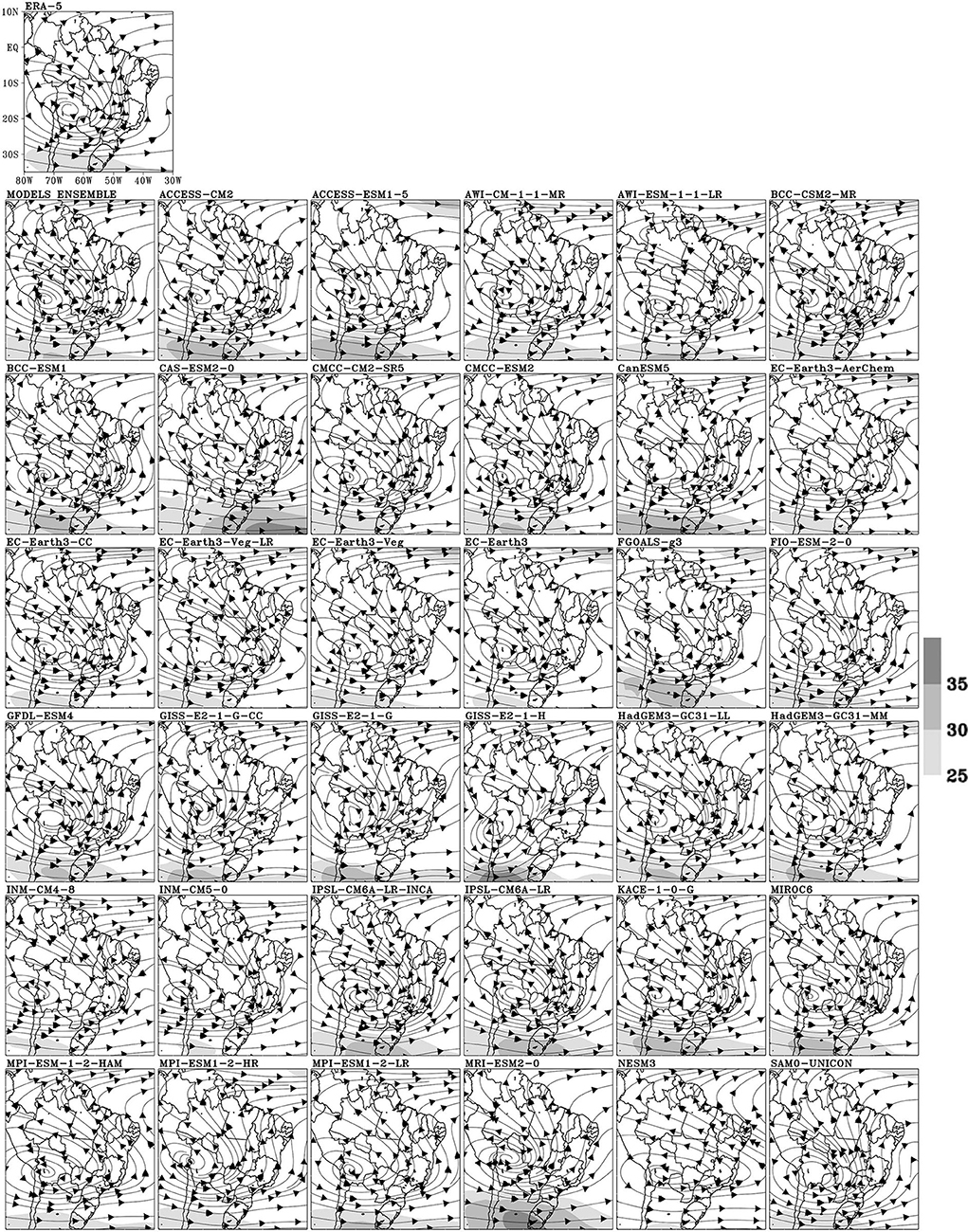
Figure 4. Streamlines and magnitude of climatological winds (m/s) at 200 hPa simulated by the multi-model ensemble mean, individual CMIP6 models, and ERA-5 reanalysis (top left) for austral summer (DJF) during the historical period. The shaded regions represent wind magnitude starting from 5 m/s while the vector shows the wind direction.

During austral winter, the circulation at upper levels is predominantly zonal over SA (Figure 5). Counterclockwise circulation is noted crossing the equatorial region in response to intense convective activity occurring in the north of SA, in the Central American region, and in adjacent oceans. In addition, the zonal circulation over the extratropical region is more intense than during DJF, with the subtropical jets placed between 20° and 40°S. CMIP6 models and the ensemble mean reproduce the zonal circulation fairly well over extratropical and subtropical regions, although some models overestimate (e.g., MRI-ESM2-0) and others underestimate (e.g., GFDL-ESM4) the subtropical jet speed. Most models, including the ensemble mean, do not reproduce adequately the counterclockwise circulation over equatorial SA. However, this feature is present in CAS-ESM2-0, EC-Earth3 family, INM-CM4-8, INM-CM5-0, IPSL-CM6A-LR, IPSL-CM6A-LR-INCA, and MRI-ESM2-0 models.

FIGURE 5

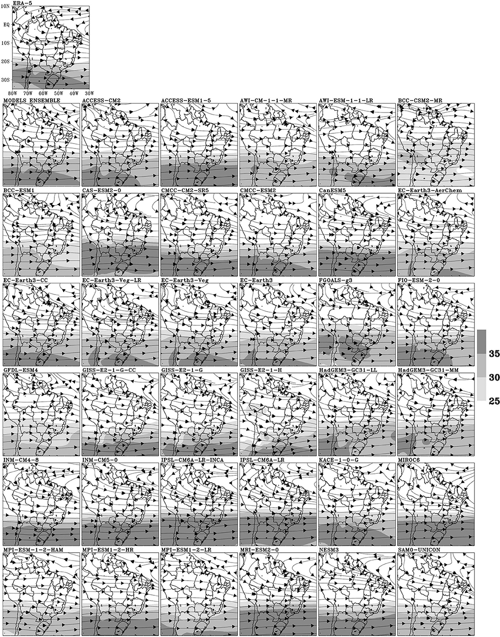
Figure 5. Streamlines and magnitude of climatological winds (m/s) at 200 hPa simulated by the multi-model ensemble mean, individual CMIP6 models, and ERA-5 reanalysis (top left) for austral winter (JJA) during the historical period. The shaded regions represent wind magnitude starting from 5 m/s while the vector shows the wind direction.

Precipitation patterns and model bias

Figure 6 shows the CRU seasonal precipitation climatology (top panel) and CMIP6 model biases (other panels) for austral summer (DJF). To quantify the similarity between each model's precipitation climatology and observed precipitation, we calculated the spatial RMSE and correlation coefficient for each GCM in relation to the observation. DJF corresponds to the rainy season over most of SA, with precipitation above 150 mm/month in most of the continent due to the South American monsoon system (Vera et al., 2006; Grimm, 2011). However, while the rainy season in Southern Amazonia occurs during DJF, as it also does in Central Brazil, associated with the Chaco Low and the South Atlantic Convergence Zone (SACZ), in Northern Amazonia, the rains are more intense in April–May, in part associated with the position of the Inter-Tropical Convergence Zone (ITCZ) (Marengo and Nobre, 2009). Northeast Brazil shows less precipitation than the other regions but has a well-defined rainy season from March to May (due to the ITCZ position) with an average seasonal precipitation of about 400 mm.

FIGURE 6

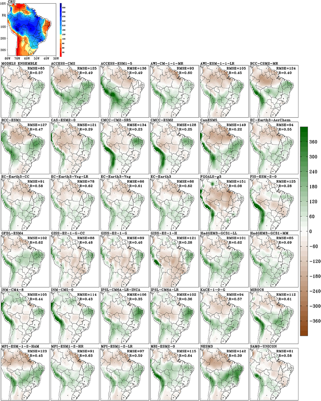
Figure 6. CMIP6 model biases and CRU-observation (top left panel) for precipitation: Austral summer (DJF). Unit: mm/month.

Most CMIP6 models including the ensemble mean show a dipolar pattern in precipitation bias over tropical Brazil, with an underestimation over the Amazon and an overestimation over Northeast Brazil. The dipolar bias is associated mainly with the wrong position of the maximum precipitation center simulated by the models over the Amazon. In general, tropical precipitation over SA is not well reproduced by CMIP6 models and is simulated too far east compared to the observed wet months over the Amazon. Some reasons are well known and include the misrepresentation of cloud physics (Khairoutdinov et al., 2005). This characteristic was reported by the studies that evaluated models from previous CMIP phases (e.g., Yin et al., 2013; Sierra et al., 2015) and by Almazroui et al. (2021a) and Ortega et al. (2021) that assessed CMIP6 models.

It is noted that the deficiency in the CMIP models exists since CMIP3 (Gulizia and Camilloni, 2015) and CMIP5 (Llopart et al., 2020), despite CMIP5 being an improvement compared to CMIP3. Overall, the CMIP5 ensemble showed improvements in the simulation of regional patterns of precipitation compared to previous generations of climate models (Sperber et al., 2013). However, although previous results suggest with confidence that models reproduce regional climate variability on a wide range of time scales well (Alves et al., 2021), some GCMs still do not represent the rainfall variability well, particularly in the tropics (Wang et al., 2014). For instance, over the Amazon Basin and Northeastern Brazil, GCMs still show a poor simulation of the current climate. This may be due to heterogeneities in the precipitation behavior within the Amazon. Precipitation in the southern portion of the Amazon is directly influenced by the South American monsoon system, whereas the precipitation in the northern sector of the basin is not influenced by the monsoon regime. da Rocha et al. (2009) found such distinct precipitation regimes after analyzing data from flux towers situated in different sectors of the Amazon. The authors showed that the onset and demise of the dry and rainy seasons as detected by the flux towers depend on the location within the Amazon. Another aspect that may explain such results is the distinct types of land cover in the Amazon that also play a direct role in influencing the onset of convection in the tropical region. As for Northeastern Brazil, rain is generated by (comparatively) shallower convection and the rainy season is influenced by easterly wave disturbances.

Northeastern Brazil is also located in the tropics, but, in contrast to the Amazon Basis, the development of deep convection is not as widespread and is not observed throughout the entire year. For the Northeastern region, these are the aspects that may explain the model deficiencies in representing the rainfall regime in that region. However, accuracy in the representation of this process in climate models is still not trivial, as indicated by Knutti and Sedlácek (2013), due to different sources of uncertainties such as potential effects of different stressors, such as land-use change and fires, ocean-atmosphere feedbacks, and high-resolution simulations which could lead to a better representation of both the spatial patterns and magnitudes of mean climate and climate extremes, especially in regions of strong surface heterogeneity (Alves et al., 2021).

In addition, the region with positive bias extends to the southeast and central regions of Brazil in some CMIP6 models (ACCESS-CM2, CanESM5, HadGEM3-GC31-LL, KACE-1-0-G, MIROC6, MPI-ESM-1-2-HAM, and NESM3). On the other hand, all models overestimate precipitation over the Andes, as reported by Almazroui et al. (2021a). In general, the best representation of DJF precipitation spatial pattern and amplitude is shown by the EC-Earth3 family (RMSE = 78, 86, 91 and 94 mm, R = 0.62, 0.61, 0.58, and 0.55) and SAM0-UNICON (RMSE = 81 mm, R = 0.58). The comparison between Figures 2, 6 suggests that the precipitation bias is also related to the deficiencies in reproducing the low-level circulation at 850 hPa over SA, and the ITCZ is often displaced southward in CMIP6 models in the austral summer (Ortega et al., 2021). One possible cause is the weaker trade winds simulated by CMIP6 models compared to ERA5, mostly over the South American east coast and the adjacent Atlantic Ocean. Due to the southward (northward) shift in the ITCZ, precipitation overestimation (underestimation) is noted over Northeast Brazil (e.g., NESM2 and MIROC6).

The positive precipitation bias over Southeast and Central Brazil regions shown by some CMIP6 models could be associated with a too intense westerly flow over the central regions of South America (south of 10°S in Figure 2) when compared to ERA5. Besides the increased heat and moisture transportation by this flow, low-level convergence is amplified over these regions, due to interaction with the SASH circulation. Conversely, some models (e.g., GISS models) underestimate the precipitation over central and Southeast Brazil. Their failure in reproducing the low-level flow convergence in these regions may explain this deviation, as shown by an easterly flow over the central regions of South America (south of 10°S), which is absent in ERA5. Therefore, the models that best reproduce the mean circulation at low levels also show the lowest precipitation bias (e.g., SAM0-UNICON). Consequently, these models tend to better reproduce the circulation at high levels (Bolivian High and a trough over northeast Brazil and the tropical South Atlantic Ocean), as they are linked to the spatial distribution of tropical latent heat sources.

During the austral winter (JJA), higher totals of precipitation occur over the extreme north of SA which is associated with the seasonal variations of the Atlantic Intertropical Convergence Zone (ITCZ) and the Walker cell (i.e., northerly displacement of the ITCZ and a weakened Walker Cell) and also by synoptic activity related to the easterly waves over the Atlantic Ocean as described by several studies (Rao and Hada, 1990; Zhou and Lau, 1998; Marengo, 2003). At the same time, other SA regions, except Southern Brazil, experience a dry season (Figure 7). Probably, due to that precipitation scarcity, it is noted that CMIP6 models show lower spatial RMSE in JJA than in DJF. The main bias concerns the underestimation of the precipitation over the extreme north of the continent, recurrent in most of the models. On the other hand, some models show a positive bias over northwestern SA (e.g., FIO-ESM-2-0, MIROC6, and IPSL models). The best results were presented by HadGEM3-GC31-LL (RMSE = 49 mm, R = 0.91) EC-Earth3 family (RMSE of 52, 54, and 55 mm, R = 0.88, 0.87, and 0.87), INM-CM4-8, and INM-CM5-0 (RMSE = 52 mm, R = 0.88) models, which were able to identify the precipitation amplitude and location over the north of SA during austral winter.

FIGURE 7

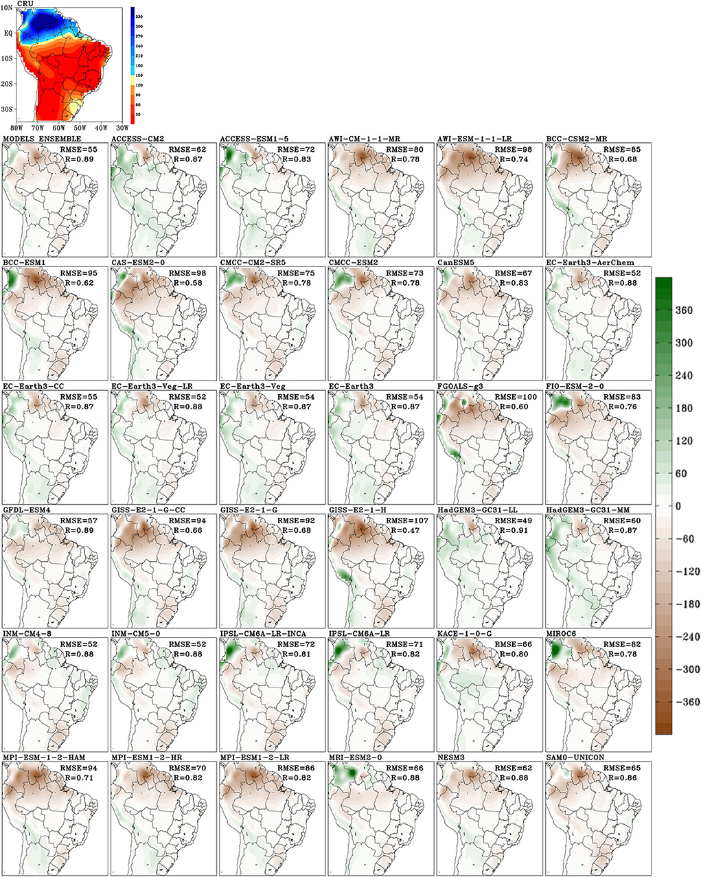
Figure 7. CMIP6 model biases and CRU-observation (top left panel) for precipitation: Austral winter (JJA). Unit: mm/month.

Surface temperature patterns and model bias

The CRU observations and CMIP6 models' biases of surface air temperature for DJF are shown in Figure 8. Overall, the mean temperature exceeds 22°C over SA during the austral summer, except over the Andes. Multi-model ensemble and CMIP6 models were consistently warmer than CRU only in the southern regions of SA. Over tropical regions, some models (e.g., EC-Earth3 models) underestimate the temperature while other models (e.g., the CanESM5 model) overestimate it. In this region, temperature biases seem to be related to precipitation biases in some models. For instance, GISS models, which show the location of maximum precipitation shifted eastward, were warmer (colder) than CRU over the Amazon region (Northeast Brazil) since precipitation and cloudiness were misrepresented. However, the relationship between temperature and precipitation biases is not evident in all models because the temperature bias is also related to errors in other processes, such as heat advection, surface interactions, and parameterizations. In general, the ensemble mean (RMSE = 2°C, R = 0.89), CMCC family (RMSE = 2.1°C, R = 0.88 and 0.89), FIO-ESM-2-0 (RMSE = 2°C, R = 0.9), HadGEM3-GC31-MM (RMSE = 2.1°C, R = 0.89), IPSL family (RMSE =2.1°C, R = 0.9), and MRI-ESM2-0 (RMSE = 2°C, R = 0.89) models display the lowest surface temperature bias for austral summer.

FIGURE 8

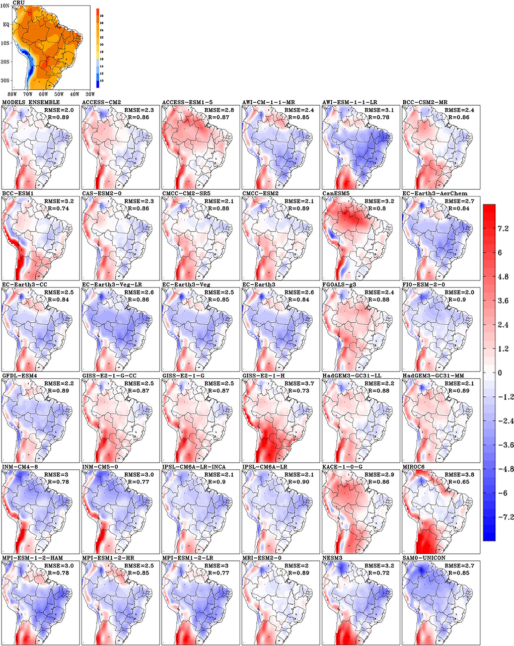
Figure 8. CMIP6 model biases and CRU-observation (top left panel) for surface air temperature: Austral summer (DJF). Unit: °C.

Figure 9 shows seasonal averages of surface air temperature and the difference between the models and observations for austral winter (JJA). CRU observations show temperatures below 20°C over extratropical regions and the Andes and up to 26°C in tropical SA regions. Most models were colder than CRU over tropical SA, especially over the eastern region. Unlike the austral summer, some models also underestimate the temperature over extratropical regions (e.g., INM models). Overall, the surface temperature bias during austral winter shows large differences in magnitude and signal among CMIP6 models. The temperature biases were the smallest for the IPSL family and the ensemble mean (RMSE = 1.8°C, R = 0.97 and 0.96) in this season.

FIGURE 9

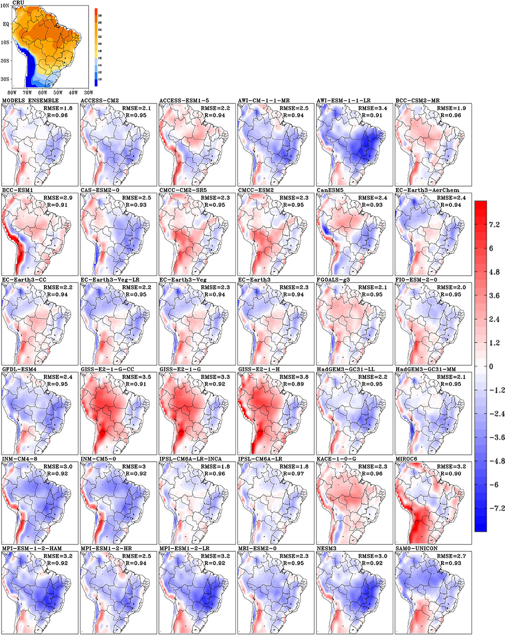
Figure 9. CMIP6 model biases and CRU-observation (top left panel) for surface air temperature: Austral winter (JJA). Unit: °C.

Frequency distributions

Beyond the model's skill to reproduce seasonal precipitation and temperature patterns discussed in previous sections, it is important to also examine their ability to reproduce climate variability. In this section, we analyze the spatiotemporal frequency distributions of monthly precipitation and surface temperature for the reference period using their PDFs. The multi-model ensemble mean is compared to the observations, demonstrating seasonal differences for each sub-region of the study.

Precipitation frequency distributions

CMIP6 GCMs' skill in representing the CRU precipitation frequency distribution is evaluated from the PDFs plotted on the top row of Figure 10. The curves were generated separately for the austral summer (DJF) and winter (JJA) over each sub-region, assuming a Gaussian distribution. In summer, the observational curves (red curves) differ according to the sub-region: For SAZ and SAM, the most likely value was about 8 mm/day, while for NAZ, it was ~7 mm/day, LPB, 5 mm/day, and NEB, 4 mm/day. Even though SAM average precipitation is close to the SAZ value, the rainy seasons are not perfectly in phase, and the peak of rainfall in SAM occurs in DJF, while in SAZ, it is in JFM. Besides these differences, NAZ and SAZ curves were flatter than the other sub-regions, indicating a higher variability in monthly precipitation, as confirmed by the SD values (about 3.3 mm/day, while the value is below 2.7 mm/day for other regions). Model observation PDF comparison shows some important differences. The frequency of months with low precipitation ( ≤ 4 mm/day) is higher for the CMIP6 ensemble than for the observed curve for NAZ, SAZ, and LPB. However, the opposite occurs over SAM and NEB, where CMIP6 ensemble curves present a higher probability of rain above 10 mm/day compared to observations. These results endorse those obtained in the previous section (Figure 6), suggesting that CMIP6 models overestimate precipitation over NEB while underestimating precipitation over the Amazon. In addition, the SD of the CMIP6 ensemble is higher than the observations for SAZ, SAM, NEB, and LPB, indicating that models simulate a more variable rainfall climate than observations. Concerning the agreement among CMIP6 models, SAM presents the largest spread, implying a higher uncertainty in the monthly mean precipitation simulations for this region.

FIGURE 10

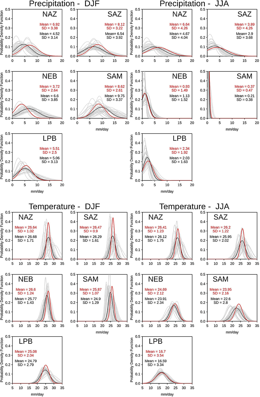
Figure 10. Probability density functions (PDF) of seasonal precipitation (top) and temperature (bottom) for Austral summer (DJF) and winter (JJA) in comparison with observations (red line) over each sub-region in the reference period. The continuous gray lines represent PDF of all GCMs and the black line is the average PDF for the GCMs (i.e., CMIP6 models).

During winter (JJA), NAZ and SAZ PDFs show the same variance (SD = 4.26 mm/day), differing only on the most likely value (6.64 mm/day to NAZ and 3.89 mm/day to SAZ), indicating more precipitation in the northern than southern Amazon in this season. There is a high frequency of near-zero precipitation values in SAM due to a well-defined dry season in this region (shown in detail in Figure 11). NEB has a most likely value of around 1 mm/day while for LPB, it is closer to 2 mm/day. The CMIP6 ensemble reproduces the observed PDF adequately for NEB but tends to underestimate the most likely values for the other regions, despite the good agreement on the variance. Generally, the results indicate that the CMIP6 ensemble simulates the precipitation frequency distribution better in winter than in summer for all regions.

FIGURE 11

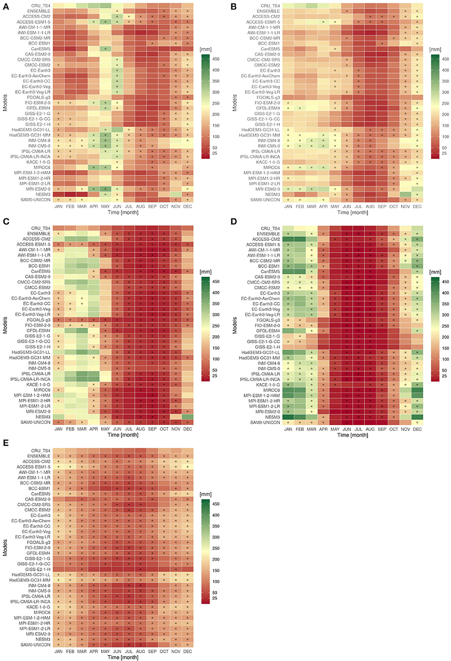
Figure 11. Portrait diagrams of the annual precipitation cycle simulated by 36 CMIP6 models and CRU TS (observational data) over the historical period in NAZ (A), SAZ (B), NEB (C), SAM (D), LPB (E). CMIP6 models' results comprised within the range of two standard deviations of the observation were highlighted with an asterisk.

Temperature frequency distributions

A similar analysis of the PDFs is done for surface air temperature (bottom of Figure 10). The observational PDFs for austral summer (DJF) indicate a most likely temperature between 26 and 27°C for NAZ, SAZ, and NEB; about 26°C for SAM and 25° for LPB. The LPB shows a flatter curve, indicating a larger variability (SD = 2.04°C) in the monthly averaged temperature. The CMIP6 ensemble is more consistent with the observations than for precipitation, despite some minor differences. For NEB and SAM, for example, the most likely values of the ensemble distribution were almost 1.0°C lower than observations. The CMIP6 SDs were higher than the observation for all regions, and NAZ and SAZ show the most significant spread of model curves. The results for winter were similar for NAZ, SAZ, and NEB. For SAM, the CMIP6 ensemble underestimates the most likely value by almost 1.5°C and also presents higher variability and spread among the models. This model limitation is not associated with a precipitation bias in this region, so this is likely to be associated with other processes. The models achieve the best results for temperature simulations over LPB, reproducing the most likely value and the variability in this region.

Annual cycle

This section analyzes how the ensemble mean and the models individually reproduce the annual cycle of precipitation and temperature in the five selected sub-regions. Hence, monthly average values from CRU data for all years and grid points (within the region) were grouped in climatology bins, ranging from January to December, and used as a reference. We defined a range of two standard deviations for each bin to settle an objective method to compare the models' skills in simulating the annual cycle. The CMIP6 models' monthly simulations within this range were highlighted (with an asterisk) in Figures 11, 12, indicating a hit (success). Thus, for each model (in each region), more asterisks indicate a better ability in simulating the annual cycle.

FIGURE 12

Figure 12. Same as in Figure 11 but for temperature.

Annual cycle of precipitation

Figure 11 shows the annual cycle of precipitation simulated by CMIP6 models over each of the study areas. CRU TS and precipitation were used as observational references.

In NAZ (Figure 11A), the HadGEM3-GC31-MM and IPSL-CM6A-LR models show better performance than others in simulating the annual precipitation cycle, despite both showing a delay in the rainy season onset of at least 1 month. In the SAZ area (Figure 11B), the HadGEM3-GC31-MM shows the best result again when analyzing the sum of hits throughout the year. Moreover, the INM-CM4-8, INM-CM5-0, and MIROC6 models show a similar ability to simulate precipitation, if we consider only the rainy season. In both Amazon regions, the CMIP6 ensemble underestimates the rainfall, especially during the rainy season. In NAZ, it also shortens the rainy season and delays its onset.

Most CMIP6 models capture the dry season pattern in NEB (Figure 11C) but overestimate precipitation during the rainy season. FIO-ESM-2-0, ACCESS-ESM1-5, FGOALS-g3, SAM0-UNICON, EC-Earth3-CC, and HadGEM3-GC31-MM were the models that best simulated the annual precipitation cycle.

In SAM (Figure 11D), most models were able to reproduce the rainy season pattern between November and January, despite the overestimation compared to observations. This is similar to the result found by Ortega et al. (2021) when analyzing the models' ability to simulate the annual precipitation cycle in the Brazilian Cerrado. Among them, IPSL-CM6A-LR-INCA and INM-CM5-0 models show the best performance in quantifying the monthly totals of precipitation.

La Plata Basin does not present a well-defined rainy season, differing from the other areas of this study. Concurrently, it is the region where the models showed the best results (Figure 11E). For LPB, GISS-E2-1-H and GISS-E2-1-G-CC models show the worst performance, underestimating the precipitation amount in most months.

Overall, most CMIP6 models simulate the seasonal behavior of precipitation over the five regions, especially in SAM and LPB. However, the models tend to underestimate the precipitation in NAZ and SAZ, both in the dry and wet periods, besides a delay of 1 or 2 months in the rainy season onset. The opposite occurs in NEB, where models tend to overestimate the precipitation amount. This bias is consistent with the shift in precipitation identified and discussed in Section Recognizing the spatial patterns. The same limitation was observed in previous CMIP model assessment studies. Almazroui et al. (2021a) found a good agreement in evaluating the CMIP6 GCMs ensemble mean annual precipitation cycle over SA. Despite that, some regions of the Northeast, South, Central, and part of southern Amazon showed large biases, indicating over (under) estimation during the wet (dry) season. Concerning the lags, Rivera and Arnould (2020) also noted a delay of 1 month in maximum precipitation in several CMIP6 models when reproducing the annual cycle in the north of southwestern South America.

Annual cycle of temperature

Figure 12 shows the surface temperature annual cycle, obtained from the same procedure as for precipitation in Figure 11. In the NAZ and SAZ regions (Figures 12A,B), the models adequately simulate the mean temperature behavior during the austral summer but underestimate (overestimate) it during the winter (spring). Some models such as BCC-ESM1, CMCC-CM2-SR5, MIROC6, and MPI-ESM1-2HR e MRI-ESM2-0 partially simulated the observed characteristics, but CMCC-ESM2 performed slightly better, based on the number of hits. In SAZ, the models show a lower ability to simulate the annual temperature cycle compared to NAZ.

Most models could simulate the temperature seasonal behavior in NEB (Figure 12C). CMCC-ESM2 and FGOALS-g3 models, for example, simulated the annual temperature cycle well. BCC-CSM2-MR, CMCC-CM2-SR5, MRI-ESM2-0, GISS-E2-1-G, and GISS-E2-1-G-CC also showed good performance for 10 or more months. Underestimates were centered in the winter months (JJA) for most models.

For the SAM region (Figure 12D), a few models adequately simulate the temperature annual cycle, while most of them underestimate temperature in the winter months and overestimate it in spring. These results were similar to those of Ortega et al. (2021) for the Brazilian Cerrado, using ERA5 as the observational reference. In our case, BCC-CSM2-MR, BCC-ESM1, ACCESS-ESM1-5, CMCC-CM2-SR5, and FIO-ESM-2-0 showed outstanding performance. Fan et al. (2020) also observed this tendency to underestimate the winter temperature for SA when evaluating the global performance of CMIP6 models.

For LPB, models showed a better ability at simulating the annual temperature cycle (Figure 12E), especially for austral winter (JJA). Among 35 CMIP6 models analyzed by this study, 15 (ACCESS-ESM1-5, CanESM5, CMCC-CM2-SR5, CMCC-ESM2, EC-Earth3, EC-Earth3-CC, EC-Earth3-Veg, FGOALS-g3, FIO-ESM-2-0, GFDL-ESM4, HadGEM3-GC31-LL, HadGEM3-GC31-MM, IPSL-CM6A-LR, IPSL-CM6A-LR-INCA, and MRI-ESM2-0) simulate the annual cycle of temperature well, as well as the ensemble mean.

Models' performance

To quantify the models' performance and identify the best ones at simulating temperature and precipitation over Brazil, two approaches were adopted: model ranking based on the annual cycle simulations presented in Figures 11, 12, and Taylor diagrams analysis, accounting for spatial correlation, RMSE, and standard deviation.

Annual cycle ranking

To quantify and compare the model's ability to simulate the annual cycle, we ranked the 35 models and the ensemble based on their hit scores (Figure 13). The hit score was defined as the percentage of hits (asterisks) calculated from Figure 11 (precipitation) and Figure 12 (temperature), considering all five regions. For precipitation (left of Figure 13), HadGEM3-GC31-MM showed the best performance (hit score of 91.7%), followed by ACCESS-ESM1-5, IPSL-CM6A-LR (78.3%), and IPSL-CM6A-LR-INCA, INM-CM4-8, INM-CM5-0, and MRI-ESM2-0 (~75%). Remarkably, the ensemble mean was in the 19th position, presenting a hit score of 61.7%, which suggests a substantial impact of under-performing models. Nonetheless, it is important to note that 30 out of 36 models showed a hit score equal to or higher than 50% for the five regions combined, indicating that most models reproduce the annual precipitation cycle for Brazil.

FIGURE 13

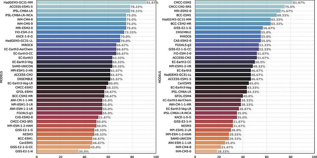
Figure 13. Ranking of CMIP6 models based on the skill of the models simulates the precipitation (left) and temperature (right) annual cycle for the historical period (1995–2014) over five-study regions. The values correspond to the percentage of hits (hit score) based on Figure 11 (precipitation) and Figure 12 (temperature).

Concerning surface temperature, CMCC-ESM2, CMCC-CM2-SR5, MRI-ESM2-0, BCC-ESM1, and HadGEM3-GC31-MM were the top five models in the five key regions (right of Figure 13). The ensemble mean was in the eighth position and a total of 14 models showed a hit score above 50% for the annual temperature cycles.

In summary, these results support the proposition that, despite the fact that combining model outputs may generally increase the skill of simulations, as suggested by some studies (Knutti et al., 2010; Raju and Kumar, 2020), selecting a subset of top-ranked models could lead to better results. This strategy can outperform the multi-model ensemble means as well as the best single GCM as discussed by Ahmed et al. (2020).

Precipitation Taylor diagram

Figure 14 (top row) summarizes the degree of spatial correspondence between the precipitation observed (CRU) and simulated by the CMIP6 models, considering the austral summer (DJF) and winter (JJA), respectively, for the five sub-regions analyzed in this study. For DJF (top and left of Figure 14), the CMIP6 ensemble mean of precipitation shows good agreement with the observations. The sub-regions show correlation values for the ensemble mean of about 0.8 (NAZ, SAZ, and SAM), and 0.9 (LPB), with the worst performance for the NEB region (R~0.6). Most models have a spatial correlation between 0.6 and 0.8 over NAZ and SAZ and between 0.7 and 0.95 over LPB. For NEB and SAM, the models present a large spread (0 to 0.9), so some models were excluded from the plots due to a negative correlation coefficient: GISS-E2-1-G, GISS-E2-1-G-CC, GISS-E2-1-H, and NESM3 for the NEB region and CanESM5, IPSL-CM6A-LR e IPSL-CM6A-LR-INCA for the SAM region. Other regional differences were related to the standard deviation, which has values around 0.25 over NAZ, NEB, and SAM; and 1.25 over SAZ and LPB for the ensembles. The best performances for the ensemble RMSE were over LPB (~0.5) and NAZ (~0.6), where the models also showed more consistency, with RMSE varying from 0.5 to 1 for most models. Generally, the CMIP6 models were more skillful over LPB and showed poor performance and a large spread over NEB. Some outstanding models were highlighted by sub-region: GFDL-ESM4, CMCC_CM2-SR5, BCC-CSM2-MR, GISS- E2-1-G, INM-CM4-8 (LPB); EC-Earth3-Veg-LR, CMCC-CM2, FIO-ESM-2-0 (NAZ); SAM0-UNICON, EC-Earth3-Veg-LR, HadGEM3-GC31-MM (SAZ); EC-Earth3-Veg-LR, MRI-ESM2-0, MPI-ESM1-2-HR (SAM); SAM0-UNICON, ACCESS-ESM1-5, and HadGEM3-GC31-MM (NEB).

FIGURE 14

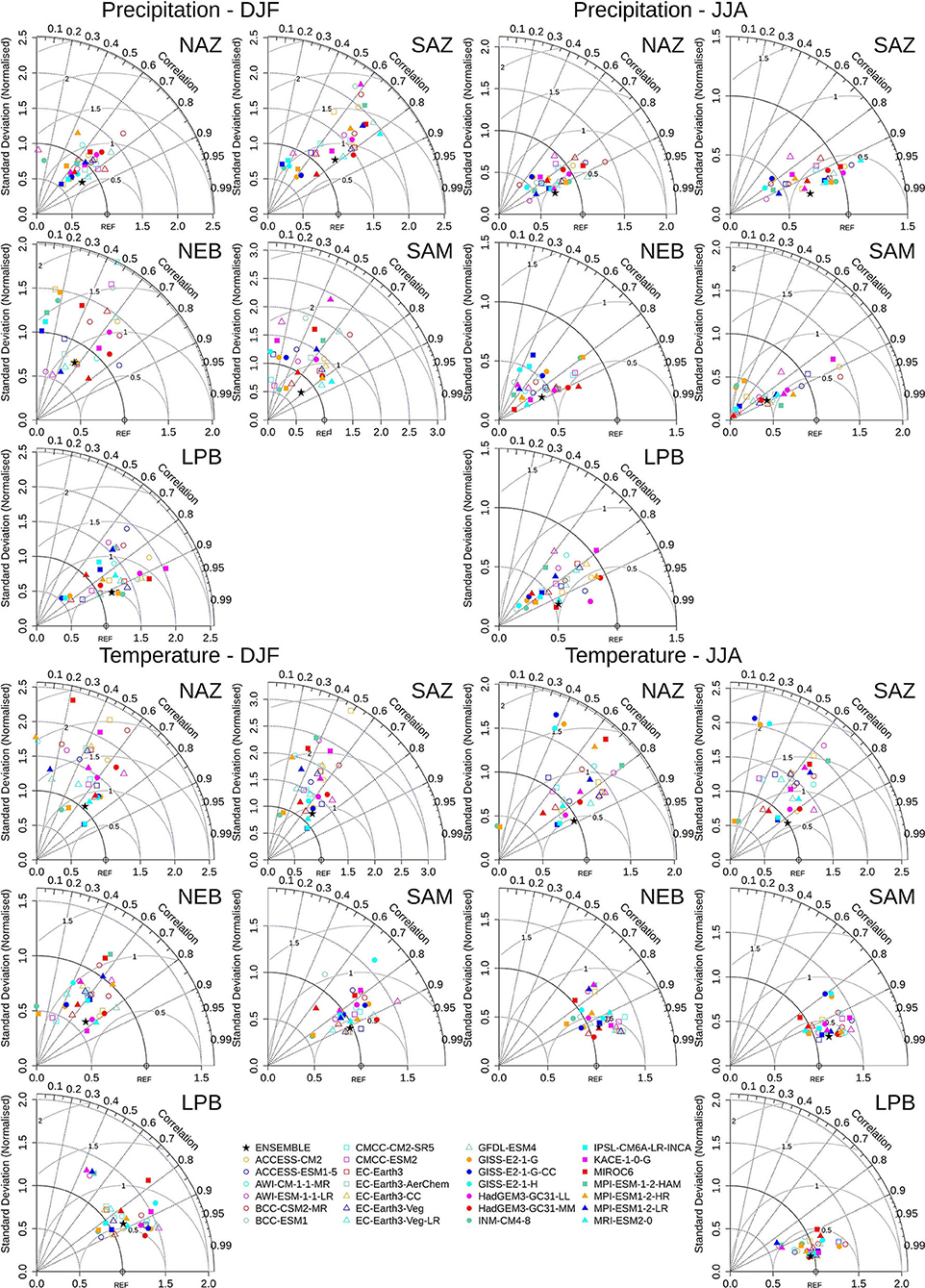
Figure 14. The Taylor diagram for CMIP6 models precipitation (top) and temperature (bottom) simulation in summer (DJF) (left) and winter (JJA) (right) over each sub-region. The angular coordinate at the right side of each diagram corresponds to the R; the radial distance from the origin represents the ratio of the standard deviation of the simulation to that of the observation, and the distance from the reference point (observations) is a measure of the RMSE.

In the winter (JJA), the CMIP6 models show a high correlation over all the sub-regions. The correlation coefficients range from 0.6 to 0.9 for most models, with the ensemble mean achieving values above 0.9 for the five sub-domains. Nonetheless, for all the sub-regions, most models present a normalized standard deviation between 0 and 1, which means that the simulated standard deviation is lower than the observed. This is consistent with the results from Figure 10, indicating that most models underestimate extreme monthly precipitation events during winter (JJA). At last, the RMSE varies between 0.5 and 1, except for SAZ, where the RMSE is lower than 0.7, evidencing a better spatial correlation of precipitation.

Temperature Taylor diagram

Figure 14 (bottom) shows the Taylor diagrams for DJF and JJA for surface air temperature. Generally, the models show worse performance and a large spread in simulating temperature over the Amazon (NAZ and SAZ) in DJF than over other sub-regions. The correlation coefficient was about 0.65 for the ensemble mean, while it ranges from 0 to 0.8 for individual models. Despite a relatively low difference between standard deviations of ensembles and observation (ratio close to 1), most models show higher values, ranging from 0.75 to 2.5 over both sub-regions. The RMSE agreed with other metrics, with values between 1 and 2 for most models, reaching values near 1 for the ensemble mean. Three models show outstanding performance for DJF temperature over NAZ and SAZ: IPSL-CM6A-LR, IPSL-CM6A-LR-INCA, and MRI-ESM2-0. Summer temperature simulations for NEB show slightly better performance, with an ensemble correlation coefficient of about 0.82 (ranging from 0.4 to 0.8), a standard deviation of 0.6 (0.5 to 1), and an RMSE of 0.6 (0.5 to 1). GFDL-ESM4, HadGEM3-GC31-MM, and CanESM5 achieve the best results. CMIP6 models perform even better over the SAM region, where the ensemble presented a correlation coefficient of 0.91 (ranging from 0.7 to 0.95), combined with a standard deviation close to the reference (ranging from 0.7 to 1.3) and an RMSE <0.5 (ranging from 0.3 to 0.8 for most models). For SAM, the models with the best performance were EC-Earth3-AerChem, EC-Earth3, EC-Earth3-Veg, and EC-Earth3-CC. The best results were found over LPB again, with a correlation around 0.88 (0.75 to 0.85), a relative standard deviation of 1.2 (1 to 1.5), and an RMSE of 0.6 (0.5 to 0.8), with the models FIO-ESM-2-0, CanESM5 and HadGEM3-GC31-MM outstanding.

CMIP6 models demonstrated better performance in simulating winter than summer temperatures. NAZ and SAZ show similar results again. The multi-model ensemble shows a good correlation for these regions, with coefficients of 0.89 and 0.83, but a wide spread among individual models (0 to 0.9). The ensemble standard deviations were similar to the observation over both sub-regions (ratio close to 1). The RMSE was close to 0.5, with a large spread among the models. The best models for simulating winter temperature over NAZ and SAZ were HadGEM3-GC31-LL, IPSL-CM6A-LR, and IPSL-CM6A-LR-INCA. The ensemble mean performance was also similar over NEB and SAM, with a correlation coefficient of 0.92 and 0.96, respectively, a normalized standard deviation of about 1.2, and an RMSE of <0.5. Most models present a relatively good consistency, ranging from 0.8 to 0.98 for correlation coefficient, 0.8 to 1.5 for standard deviation, and 0.2 to 0.8 for RMSE. FIO-ESM-2-0 and HadGEM3-GC31-MM provided the best simulations over NEB while IPSL-CM6A-LR and CAS-ESM2-0 over SAM. The ensemble mean shows a high correlation (0.98) for LPB, combined with a standard deviation close to 1 and a low RMSE (0.2). Most models also presented a good consistency (correlation coefficient above 0.9, standard deviation from 0.6 to 1.4, and RMSE below 0.5). EC-Earth3-CC, EC-Earth3-Veg, MRI-ESM2-0, and HadGEM3-GC31-MM showed the best performance.

We note that some CMIP6 models show limitations in simulating precipitation and temperature for DJF and JJA over the five sub-regions in Brazil, despite the good performance of the ensemble mean. During winter, we found the best results, especially for LPB, followed by SAM and NEB. Over NAZ and SAZ, models demonstrated similar ability for temperature simulations, but important differences for precipitation skill, despite the proximity between these regions.

Summary and conclusion

There is now a wide range of climate projections that can be used across a number of sectors. However, it is essential to assess the skill of projections to ensure they are appropriate for their intended use. In this study, we provide a comprehensive assessment of precipitation, circulation, and temperature simulations of 35 CMIP6 models over Brazil during the present day. First, we analyzed atmospheric circulation patterns in the austral summer (DJF) and winter (JJA) seasons. The main findings indicate that many models showed large-scale deficiencies in reproducing the SALLJ, an important mechanism transporting heat and moisture from low to high latitudes in DJF over Brazil.

The spatial analysis of rainfall shows a systematic bias in the CMIP6 model simulations, with an underestimation of the mean precipitation during summer over NAZ and SAZ and an overestimation over Northeast Brazil, and this is might be partially related to model limitations in simulating cloud physics (Khairoutdinov et al., 2005). Overall, this result is in line with previous regional studies (Yin et al., 2013; Sierra et al., 2015; Almazroui et al., 2021a; Ortega et al., 2021).

Although they exhibit systematic bias, some robust conclusions still emerge from the PDF of precipitation, which showed that the CMIP6 models reproduce the winter PDFs better than the summer ones, when they increase the frequency of extremes. Among all regions, models converge and better reproduce the precipitation PDF over LPB, whereas the highest spread occurs over SAM. This suggests that SAM is the most challenging region for precipitation simulation over the study area.

For temperature, there is a high spread among models. However, the ensemble underestimates the temperature over Northeast and Central Brazil, consistent with the systematic precipitation bias. Most models perform better in simulating the monthly surface temperature distributions than precipitation, especially over LPB.

The annual precipitation cycle simulated by most CMIP6 models showed a 1- to 2-month shift in the rainy season over NAZ and SAZ. This shift may cause the precipitation deficit identified in summer over the same regions (Figures 6, 10). On the other hand, the models adequately capture the annual cycle over NEB but overestimate the precipitation during wet months. CMIP6 models better reproduce the annual precipitation cycle over SAM and LPB.

Another important outcome is that most models overestimate temperature over NAZ, SAZ, and SAM while underestimating it in the winter over SAM. The annual cycle of temperature over LPB presented higher thermal amplitude and was well simulated by most of the models.

The models with the highest ability in simulating monthly precipitation (higher hit score), aggregating all five regions, were HadGEM3-GC31-MM, ACCESS-ESM1-5, IPSL-CM6A-LR, IPSL-CM6A-LR-INCA, and INM-CM4-8, whereas, for monthly temperature, they were CMCC-ESM2, CMCC-CM2-SR5, MRI-ESM2-0, BCC-ESM1, and HadGEM3-GC31-MM. Remarkably, the CMIP6 ensemble mean is not included among the best-performing models, which suggests that selecting a subset of top-ranked models could lead to better results than the ensemble mean.

The Taylor diagram shows how CMIP6 models represent spatial patterns inside each sub-region. Based on these results, it was noted that models perform better for winter precipitation than summer. In both seasons, the worst performance was found for NEB. Results also show that the model presents deficiencies in simulating temperature in both Amazonian regions. The results also confirm previous studies with LPB showing good overall performance for precipitation and temperature.

This study has identified the best subset of CMIP6 models in simulating the mean precipitation and temperature over Brazil, although some systematic biases were found, and the highest skill depends on the area and/or season. In addition, performance will depend on the metrics adopted. For instance, some models may present a strong mean bias in some areas but capture the onset and duration of the rainy season adequately. Finally, despite the limitations intrinsic to the climate modeling process, the CMIP6 dataset offers opportunities to advance climate change science and enable decision-makers to better prepare the Brazilian society for climate change issues based on these results.

Data availability statement

Publicly available datasets were analyzed in this study. This data can be found at: ERA5 (https://www.ecmwf.int/en/forecasts/datasets/reanalysis-datasets/era5, accessed November 11, 2021), CRU TS (https://crudata.uea.ac.uk/cru/data/hrg/cru_ts_4.05/, accessed November 26, 2021), historical data for the 35 CMIP6 models from Earth System Grid Federation (https://esgf-node.llnl.gov/search/cmip6/, accessed 03 November 2021).

Author contributions

MF, LA, BG, and GO idealized the paper and wrote it. MF, BG, MS, and LD contributed to the elaboration, analyses, and discussion of maps. MF, LA, RC, ML, and GO contributed to the discussions and proofreading of this manuscript. All authors contributed to the article and approved the submitted version.

Funding

MF was supported by Conselho Nacional de Desenvolvimento Científico e Tecnológico (CNPq–no 380844/2021-4) under the project AdaptaBrasil MCTI. LA and GO are supported by São Paulo Research Foundation (FAPESP, grant 20215/50122-0) and the National Institute of Science and Technology for Climate Change Phase 2 under CNPq (grant no. 465501/2014-1). RC was supported by the Newton Fund through the Met Office Climate Science for Service Partnership Brazil (CSSP Brazil).

Acknowledgments

We acknowledge the World Climate Research Programme's Working Group on Coupled Modeling, which is responsible for CMIP, and we thank the climate modeling groups (listed in Table 1) for producing and making available their model output. For CMIP, the U.S. Department of Energy's Program for Climate Model Diagnosis and Intercomparison provides coordinating support and led the development of software infrastructure in partnership with the Global Organization for Earth System Science Portals. We acknowledge also the CSSP-Brazil for the contribution of RC.

Conflict of interest

The authors declare that the research was conducted in the absence of any commercial or financial relationships that could be construed as a potential conflict of interest.

Publisher's note

All claims expressed in this article are solely those of the authors and do not necessarily represent those of their affiliated organizations, or those of the publisher, the editors and the reviewers. Any product that may be evaluated in this article, or claim that may be made by its manufacturer, is not guaranteed or endorsed by the publisher.

References

Ahmed, K., Sachindra, D. A., Shahid, S., Iqbal, Z., Nawaz, N., and Khan, N. (2020). Multi-model ensemble predictions of precipitation and temperature using machine learning algorithms. Atmospheric Res. 236, 104806. doi: 10.1016/j.atmosres.2019.104806

PubMed Abstract | CrossRef Full Text | Google Scholar

Alfieri, L., Bisselink, B., Dottori, F., Naumann, G., de Roo, A., Salamon, P., et al. (2017). Global projections of river flood risk in a warmer world. Earth's Future. 5, 171–182. doi: 10.1002/2016EF000485

CrossRef Full Text | Google Scholar

Almazroui, M., Ashfaq, M., Islam, M. N., Rashid, I. U., Kamil, S., Abid, M. A., et al. (2021a). Assessment of CMIP6 performance and projected temperature and precipitation changes over South America. Earth Syst. Environ. 5, 155–183. doi: 10.1007/s41748-021-00233-6

CrossRef Full Text | Google Scholar

Almazroui, M., Islam, M. N., Saeed, F., Saeed, S., Ismail, M., Ehsan, M. A., et al. (2021b). Projected changes in temperature and precipitation over the United States, Central America, and the Caribbean in CMIP6 GCMs. Earth Syst. Environ. 5, 1–24. doi: 10.1007/s41748-021-00199-5

CrossRef Full Text | Google Scholar

Almazroui, M., Saeed, F., Saeed, S., Nazrul Islam, M., Ismail, M., Klutse, N. A. B., et al. (2020a). Projected change in temperature and precipitation over Africa from CMIP6. Earth Syst. Environ. 4, 455–475. doi: 10.1007/s41748-020-00161-x

CrossRef Full Text | Google Scholar

Almazroui, M., Saeed, S., Saeed, F., Islam, M. N., and Ismail, M. (2020b). Projections of Precipitation and Temperature over the South Asian Countries in CMIP6. Earth Syst. Environ. 4, 297–320. doi: 10.1007/s41748-020-00157-7

CrossRef Full Text | Google Scholar

Alves, L. M., Chadwick, R., Moise, A., Brown, J., and Marengo, J. A. (2021). Assessment of rainfall variability and future change in Brazil across multiple timescales. Int. J. Climatol. 41, E1875–E1888. doi: 10.1002/joc.6818

CrossRef Full Text | Google Scholar

Andrade, K. M., and Cavalcanti, I. F. A. (2004). “Climatologia dos sistemas frontais e padrões de comportamento para o verão na América do Sul,” in XIII Congresso Brasileiro de Meteorologia, 13, Fortaleza. Anais do XIII Congresso Brasileiro de Meteorologia.

Google Scholar

Ashfaq, M., Cavazos, T., Reboita, M. S., Torres-Alavez, J. A., Im, E. S., Olusegun, C. F., et al. (2021). Robust late twenty-first century shift in the regional monsoons in RegCM-CORDEX simulations. Climate Dyn. 57, 1463–1488. doi: 10.1007/s00382-020-05306-2

CrossRef Full Text | Google Scholar

Baettig, M. B., Wild, M., and Imboden, D. M. (2007). A climate change index: where climate change may be most prominent in the 21st century. Geophys. Res. Lett. 34, L01705. doi: 10.1029/2006GL028159

CrossRef Full Text | Google Scholar

Bannister, D., Herzog, M., Graf, H. F., Scott Hosking, J., and Short, C. A. (2017). An assessment of recent and future temperature change over the Sichuan basin, China, using CMIP5 climate models. J. Climate 30, 6701–6722. doi: 10.1175/JCLI-D-16-0536.1

CrossRef Full Text | Google Scholar

Chadwick, R., Good, P., Andrews, T., and Martin, G. (2014). Surface warming patterns drive tropical rainfall pattern responses to CO 2 forcing on all timescales. Geophys. Res. Lett. 41, 610–615. doi: 10.1002/2013GL058504

CrossRef Full Text | Google Scholar

Cook, B. I., Mankin, J. S., Marvel, K., Williams, A. P., Smerdon, J. E., and Anchukaitis, K. J. (2020). Twenty-first century drought projections in the CMIP6 forcing scenarios. Earth's Future 8, e2019EF001461. doi: 10.1029/2019EF001461

CrossRef Full Text | Google Scholar

da Rocha, R. P., Morales, C. A., Cuadra, S. V., and Ambrizzi, T. (2009). Precipitation diurnal cycle and summer climatology assessment over South America: An evaluation of Regional Climate Model version 3 simulations. J. Geophys. Res. 114, D10108. doi: 10.1029/2008JD010212

CrossRef Full Text | Google Scholar

Díaz, L. B., Saurral, R. I., and Vera, C. S. (2021). Assessment of South America summer rainfall climatology and trends in a set of global climate models large ensembles. Int. J. Climatol. 41, E59–E77. doi: 10.1002/joc.6643

CrossRef Full Text | Google Scholar

Eyring, V., Bony, S., Meehl, G. A., Senior, C. A., Stevens, B., Stouffer, R. J., et al. (2016). Overview of the coupled model intercomparison project phase 6 (CMIP6) experimental design and organization. Geosci. Model Develop. 9, 1937–1958. doi: 10.5194/gmd-9-1937-2016

CrossRef Full Text | Google Scholar

Fan, X., Duan, Q., Shen, C., Wu, Y., and Xing, C. (2020). Global surface air temperatures in CMIP6: historical performance and future changes. Environ. Res. Lett. 15, 104056. doi: 10.1088/1748-9326/abb051

CrossRef Full Text | Google Scholar

Fischer, E. M., and Knutti, R. (2016). Observed heavy precipitation increase confirms theory and early models. Nat. Climate Change 6, 986–991. doi: 10.1038/nclimate3110

CrossRef Full Text | Google Scholar

Flato, G. J, Marotzke, B., Abiodun, P., Braconnot, S. C., Chou, W., et al. (2013). “Evaluation of Climate Models,” in Climate Change 2013: The Physical Science Basis, Contribution of Working Group I to the Fifth Assess- ment Report of the Intergovernmental Panel on Climate Change, eds T. F. Stocker, D. Qin, G.-K. Plattner, M. Tignor, S.K. Allen, J. Boschung, A. Nauels, Y. Xia, V. Bex and P.M. Midgley (Cambridge U).

Google Scholar

Grimm, A. M. (2011). Interannual climate variability in South America: impacts on seasonal precipitation, extreme events, and possible effects of climate change. Stochastic Environ. Res. Risk Assess. 25, 537–554. doi: 10.1007/s00477-010-0420-1

CrossRef Full Text | Google Scholar

Gulizia, C., and Camilloni, I. (2015). Comparative analysis of the ability of a set of CMIP3 and CMIP5 global climate models to represent precipitation in South America. Int. J. Climatol. 35, 583–595. doi: 10.1002/joc.4005

CrossRef Full Text | Google Scholar

Gusain, A., Ghosh, S., and Karmakar, S. (2020). Added value of CMIP6 over CMIP5 models in simulating Indian summer monsoon rainfall. Atmospheric Res. 232, 104680. doi: 10.1016/j.atmosres.2019.104680

CrossRef Full Text | Google Scholar

Harris, I., Jones, P. D., Osborn, T. J., and Lister, D. H. (2014). Updated high-resolution grids of monthly climatic observations - the CRU TS3.10 Dataset. Int. J. Climatol. 34, 623–642. doi: 10.1002/joc.3711

CrossRef Full Text | Google Scholar

Harris, I., Osborn, T. J., Jones, P., and Lister, D. (2020). Version 4 of the CRU TS monthly high-resolution gridded multivariate climate dataset. Sci. Data 7, 109. doi: 10.1038/s41597-020-0453-3

PubMed Abstract | CrossRef Full Text | Google Scholar

Held, I. M., and Soden, B. J. (2006). Robust responses of the hydrological cycle to global warming. J. Climate 19, 5686–5699. doi: 10.1175/JCLI3990.1

CrossRef Full Text | Google Scholar

Hersbach, H., Bell, B., Berrisford, P., Hirahara, S., Horányi, A., Muñoz-Sabater, J., et al. (2020). The ERA5 global reanalysis. Quarterly J. Royal Meteorol. Soc. 146, 1999–2049. doi: 10.1002/qj.3803

CrossRef Full Text | Google Scholar

IPCC (2021). Climate Change 2021 The Physical Science Basis Summary for Policymakers Working Group I Contribution to the Sixth Assessment Report of the Intergovernmental Panel on Climate Change, Climate Change 2021: The Physical Science Basis.

Google Scholar

Khairoutdinov, M., Randall, D., and DeMott, C. (2005). Simulations of the atmospheric general circulation using a cloud-resolving model as a superparameterization of physical processes. J. Atmospheric Sci. 62, 2136–2154. doi: 10.1175/JAS3453.1

CrossRef Full Text | Google Scholar

Knutti, R., Furrer, R., Tebaldi, C., Cermak, J., and Meehl, G. A. (2010). Challenges in combining projections from multiple climate models. J. Climate 23, 2739–2758. doi: 10.1175/2009JCLI3361.1

PubMed Abstract | CrossRef Full Text | Google Scholar

Knutti, R., and Sedlácek, J. (2013). Robustness and uncertainties in the new CMIP5 climate model projections. Nat. Clim. Chang. 3, 369–373. doi: 10.1038/nclimate1716

CrossRef Full Text | Google Scholar

Lenters, J. D., and Cook, K. H. (1997). On the origin of the Bolivian high and related circulation features of the South American climate. J. Atmospheric Sci. 54, 656–677.

Google Scholar

Llopart, M., Domingues, L. M., Torma, C., Giorgi, F., da Rocha, R. P., Ambrizzi, T., et al. (2021). Assessing changes in the atmospheric water budget as drivers for precipitation change over two CORDEX-CORE domains. Climate Dyn. 57, 1615–1628. doi: 10.1007/s00382-020-05539-1

CrossRef Full Text | Google Scholar

Llopart, M., Simões Reboita, M., and Porfírio da Rocha, R. (2020). Assessment of multi-model climate projections of water resources over South America CORDEX domain. Climate Dyn. 54, 99–116. doi: 10.1007/s00382-019-04990-z

CrossRef Full Text | Google Scholar

Luo, N., Guo, Y., Gao, Z., Chen, K., and Chou, J. (2020). Assessment of CMIP6 and CMIP5 model performance for extreme temperature in China. Atmospheric Oceanic Sci. Lett. 13, 589–597. doi: 10.1080/16742834.2020.1808430

CrossRef Full Text | Google Scholar

Lv, Y., Guo, J., Li, J., Han, Y., Xu, H., Guo, X., et al. (2021). Increased turbulence in the Eurasian upper-level jet stream in winter: past and future. Earth Space Sci. 8, e2020EA001556. doi: 10.1029/2020EA001556

CrossRef Full Text | Google Scholar

Marengo, J. A. (2003). “Condições climáticas e os recursos hídricos no norte brasileiro,” in Clima e Recursos Hídricos no Brasil, eds C. E. M. Tucci and B. P. F. Braga (Porto Alegre: Coleção ABRH), 117–156.

Google Scholar

Marengo, J. A., and Nobre, C. (2009). “Clima da Região Amazonica,” in Tempo e Clima no Brasil, 1st Edn, ed I. Cavalcanti (São Paulo: Oficina de Textos), 198–212.

Google Scholar

Marengo, J. A., Soares, W. R., Saulo, C., and Nicolini, M. (2004). Climatology of the low-level jet east of the Andes as derived from the NCEP-NCAR reanalyses: characteristics and temporal variability. J. Climate 17, 2261–2280. doi: 10.1175/1520-0442(2004)017<2261:COTLJE>2.0.CO;2

CrossRef Full Text | Google Scholar

Masson-Delmotte, V., Zhai, P., Pirani, A., Connors, S. L., Péan, C., Berger, S., et al. (2021). IPCC, 2021: Climate Change 2021: The Physical Science Basis. Cambridge University Press. In Press.

PubMed Abstract | Google Scholar

Meehl, G. A., Covey, C., Delworth, T., Latif, M., McAvaney, B., Mitchell, J. F. B., et al. (2007). The WCRP CMIP3 multimodel dataset: a new era in climatic change research. Bull. Am. Meteorol. Soc. 88, 1383–1394. doi: 10.1175/BAMS-88-9-1383

CrossRef Full Text | Google Scholar

Olauson, J. (2018). ERA5: the new champion of wind power modelling? Renew. Energy 126, 322–331. doi: 10.1016/j.renene.2018.03.056

CrossRef Full Text | Google Scholar

O'Neill, B. C., Tebaldi, C., Van Vuuren, D. P., Eyring, V., Friedlingstein, P., Hurtt, G., et al. (2016). The scenario model intercomparison project (ScenarioMIP) for CMIP6. Geosci. Model Develop. 9, 3461–3482. doi: 10.5194/gmd-9-3461-2016

CrossRef Full Text | Google Scholar

Oppenheimer, M., Glavovic, B. C., Hinkel, J., de Wal, R., Magnan, A. K., Abd-Elgawad, A., et al. (2019). Sea level rise and implications for low-lying islands, coasts and communities, IPCC special report on the ocean and cryosphere in a changing climate, edited by Pörtner, H.-O., Roberts, DC. Intergov. Panel Clim. Change. p. 321–445.

Google Scholar

Ortega, G., Arias, P. A., Villegas, J. C., Marquet, P. A., and Nobre, P. (2021). Present-day and future climate over central and South America according to CMIP5/CMIP6 models. Int. J. Climatol. 41, 6713–6735. doi: 10.1002/joc.7221

CrossRef Full Text | Google Scholar

Pereima, M. F. R., Chaffe, P. L. B., de Amorim, P. B., and Rodrigues, R. R. (2022). A systematic analysis of climate model precipitation in southern Brazil. Int. J. Climatol. 42, 4240–4257. doi: 10.1002/joc.7460

PubMed Abstract | CrossRef Full Text | Google Scholar

Raju, K. S., and Kumar, D. N. (2020). Review of approaches for selection and ensembling of GCMS. J. Water Climate Change 11, 577–599. doi: 10.2166/wcc.2020.128

CrossRef Full Text | Google Scholar

Rao, V. B., and Hada, K. (1990). Characteristics of rainfall over Brazil: Annual variations and connections with the Southern Oscillation. Theor. Appl. Climatol. 42, 81–91. doi: 10.1007/BF00868215

CrossRef Full Text | Google Scholar

Reboita, M. S., Ambrizzi, T., Silva, B. A., Pinheiro, R. F., and da Rocha, R. P. (2019). The South atlantic subtropical anticyclone: present and future climate. Front. Earth Sci. 7, 8. doi: 10.3389/feart.2019.00008

CrossRef Full Text | Google Scholar

Rivera, J. A., and Arnould, G. (2020). Evaluation of the ability of CMIP6 models to simulate precipitation over Southwestern South America: climatic features and long-term trends (1901–2014). Atmospheric Res. 241, 104953. doi: 10.1016/j.atmosres.2020.104953

CrossRef Full Text | Google Scholar

Shimizu, M. H., Anochi, J. A., and Kayano, M. T. (2022). Precipitation patterns over northern Brazil basins: climatology, trends, and associated mechanisms. Theor. Appl. Climatol. 147, 767–783. doi: 10.1007/s00704-021-03841-4

CrossRef Full Text | Google Scholar

Sierra, J. P., Arias, P. A., and Vieira, S. C. (2015). Precipitation over Northern South America and its seasonal variability as simulated by the CMIP5 models. Adv. Meteorol. 2015, 1–22. doi: 10.1155/2015/634720

CrossRef Full Text | Google Scholar

Sillmann, J., Kharin, V. V., Zhang, X., Zwiers, F. W., and Bronaugh, D. (2013). Climate extremes indices in the CMIP5 multimodel ensemble: part 1. Model evaluation in the present climate. J. Geophys. Res. Atmospheres. 118, 1716–1733. doi: 10.1002/jgrd.50203

CrossRef Full Text | Google Scholar

Sperber, K. R., Annamalai, H., Kang, I. S., Kitoh, A., Moise, A., Turner, A., et al. (2013). The Asian summer monsoon: An intercomparison of CMIP5 vs. CMIP3 simulations of the late 20th century. Clim. Dynam. 41, 2711–2744. doi: 10.1007/s00382-012-1607-6

CrossRef Full Text | Google Scholar

Srivastava, A., Grotjahn, R., and Ullrich, P. A. (2020). Evaluation of historical CMIP6 model simulations of extreme precipitation over contiguous US regions. Weather Clim. Extreme. 29, 100268. doi: 10.1016/j.wace.2020.100268

CrossRef Full Text | Google Scholar

Stouffer, R. J., Eyring, V., Meehl, G. A., Bony, S., Senior, C., Stevens, B., et al. (2017). CMIP5 scientific gaps and recommendations for CMIP6. Bull. Am. Meteorol. Soc. 98, 95–105. doi: 10.1175/BAMS-D-15-00013.1

CrossRef Full Text | Google Scholar

Su, F., Duan, X., Chen, D., Hao, Z., and Cuo, L. (2013). Evaluation of the global climate models in the CMIP5 over the Tibetan Plateau. J. Climate 26, 3187–3208. doi: 10.1175/JCLI-D-12-00321.1

PubMed Abstract | CrossRef Full Text | Google Scholar

Taylor, K. E. (2001). Summarizing multiple aspects of model performance in a single diagram. J. Geophys. Res. Atmospheres. 106, 7183–7192. doi: 10.1029/2000JD900719

CrossRef Full Text | Google Scholar

Taylor, K. E., Stouffer, R. J., and Meehl, G. A. (2012). An overview of CMIP5 and the experiment design. Bull. Am. Meteorol. Soc. 93, 485–498. doi: 10.1175/BAMS-D-11-00094.1

PubMed Abstract | CrossRef Full Text | Google Scholar

Torres, R. R., Lapola, D. M., Marengo, J. A., and Lombardo, M. A. (2012). Socio-climatic hotspots in Brazil. Climatic Change 115, 597–609. doi: 10.1007/s10584-012-0461-1

CrossRef Full Text | Google Scholar

Torres, R. R., and Marengo, J. A. (2013). Uncertainty assessments of climate change projections over South America. Theor. Appl. Climatol. 112, 253–272. doi: 10.1007/s00704-012-0718-7

CrossRef Full Text | Google Scholar

Velasco, I., and Fritsch, J. M. (1987). Mesoscale convective complexes in the Americas. J. Geophys. Res. 92, 9591–9613. doi: 10.1029/JD092iD08p09591

CrossRef Full Text | Google Scholar

Vera, C., Higgins, W., Amador, J., Ambrizzi, T., Garreaud, R., Gochis, D., et al. (2006). Toward a unified view of the American monsoon systems. J. Climate 19, 4977–5000. doi: 10.1175/JCLI3896.1

CrossRef Full Text | Google Scholar

Virji, H. (1981). A preliminary study of summertime tropospheric circulation patterns over South America estimated from cloud winds. Monthly Weather Rev. 109, 599–610.

Google Scholar

Wang, C., Zhang, L., Lee, S. K., Wu, L., and Mechoso, C. R. (2014). A global perspective on CMIP5 climate model biases. Nat. Climate Change 4, 201–205. doi: 10.1038/nclimate2118

CrossRef Full Text | Google Scholar

Yin, L., Fu, R., Shevliakova, E., and Dickinson, R. E. (2013). How well can CMIP5 simulate precipitation and its controlling processes over tropical South America? Climate Dyn. 41, 3127–3143. doi: 10.1007/s00382-012-1582-y

CrossRef Full Text | Google Scholar

Zhou, J., and Lau, K. M. (1998). Does a monsoon climate exist over South America? J. Climate 11, 1020–1040.

PubMed Abstract | Google Scholar