Application of a bivariate bias-correction approach to yield long-term attributes of Indian precipitation and temperature

Introduction

Global climate change and its impact on various regimes such as hydrology have been gaining attention among scientists and stakeholders due to its influence on land use development and other application sectors (Watson et al., 2000; Hovenga et al., 2016; Chen et al., 2018; Seo and Kim, 2018; Seo et al., 2019). The hydrological process of basins have been significantly affected by the influence of changing climate since the average global temperature has risen over the last few decades (Li et al., 2013; Jarraud and Steiner, 2014). An increased temperature typically impacts non-stationarity in hydro-meteorological variables, consequently affecting the spatio-temporal distribution of water availability (Ruelland et al., 2012; Tan et al., 2020). Former studies have reported a strong linear correlation between precipitation and temperature, two important forcing for streamflow modeling, over continents during the summer months (Zhao and Khalil, 1993; Trenberth and Shea, 2005). However, according to the Clausius-Clapeyron relationship, an increase in surface temperature would also increase precipitation, indicating a non-linear precipitation and temperature (P-T) relationship. Although an increase in extreme precipitation events attributed to climate change has been thoroughly studied, the expected changes in the linear dependency between precipitation and temperature have not been comprehensively investigated yet. Recent studies have indicated that an inappropriate estimation of the P-T linear correlation can significantly influence the long-term estimation of hydrologic fluxes (Chen et al., 2018; Seo et al., 2019). Considering these observations, General Circulation Model (GCM) outputs are essential to understand the future changes in the P-T relationship under different global greenhouse gas emission scenarios.

GCMs are widely utilized to assess the impact of global climate change on the hydrosphere as they simulate/project the physical process of climate systems (Singh et al., 2000; Campbell et al., 2011; Tan et al., 2020). Assessment Report 5 of the Coupled Model Intercomparison Project (CMIP5), which is an inter-governmental panel on climate change, provides the future climate projections under multiple representative concentration pathways (RCPs) (Taylor et al., 2012). However, GCM outputs cannot be forced into hydrologic models as they exhibit significant systematic bias, which can be a major source of uncertainty in long-term hydrologic simulations/projections (Li et al., 2014; Cannon, 2016; Tan et al., 2020). The authors note that several other factors could restrict the direct application of GCM outputs, primarily in hydrologic models, such as resolution mismatch, initial model drift, etc. Nevertheless, the bias in GCM outputs arises from an inaccurate representation of the physical process in climate models. Maraun (2016) reported that GCM outputs exhibit spatio-temporal bias in yielding the mean and the standard deviation of the observed precipitation and temperature. Ullah et al. (2020) found that the GCM efficiently simulates the observed mean temperature over South Asia, but it exhibits a large bias in yielding the standard deviation. Wang et al. (2020) noted that the mean precipitation is better reproduced by GCMs as compared to variance. Although significant efforts have been made to estimate the bias in the mean and the standard deviation in simulated variables, only a few studies have tried to estimate the bias in higher-order moments. Therefore, bias-correction approaches, whether univariate or bivariate, primarily focus on reducing the bias in the mean and the standard deviation of the simulated variable, while mostly leaving out the bias in the cross-correlation.

Bias-correction (BC) methods are mainly classified into two groups; the simple scaling technique comprises linear scaling and the power transformation method, which is a sophisticated distribution mapping method with an empirical cumulative distribution function to adjust the meteorological variables (Graham et al., 2007; Maraun et al., 2010; Piani et al., 2010; Teutschbein and Seibert, 2013). Several statistical BC approaches have been developed and validated in various parts of the world, at a basin or at the regional scale, to correct the biases in weather forecasts and long-term climate simulations. Common bias-correction techniques may vary from a traditional quantile mapping to state-of-the-art machine learning algorithms such as Support Vector Machines and Random Forest (Ghosh and Mujumdar, 2006, 2007, 2008). A deep learning-based convolution neural network (CNN) was recently applied for statistical downscaling and bias correction of temperature and precipitation in Europe (Baño-Medina et al., 2020). Apart from the advances in bias-correction techniques, researchers have also considered multivariate bias-correction approaches that simultaneously reduce bias in multiple variables while also yielding their interdependence. For example, constructed analogs-based approaches such as localized constructed analogs (LOCA) and Multivariate adapted constructed analogs (MACA) are commonly considered for multivariate bias correction (Abatzoglou and Brown, 2012; Pierce et al., 2014, 2015). Das Bhowmik et al. (2018) proposed an asynchronous Canonical Correlation (ACCA) approach to yield the cross-correlation between precipitation and temperature. However, the ACCA exhibited a major limitation in yielding the monthly variation in precipitation; albeit, it improves the joint probability of multiple variables. He et al. (2012) suggested a bivariate technique based on bivariate ranking (referred to as Bivariate Asynchronous Bias Correction or BABC) and applied the approach at the basin level. BABC has shown significant promise in yielding the monthly variation in precipitation and its cross-correlation with temperature. However, BABC requires comprehensive validation that incorporates a continental scale and multiple GCM ensembles. A comprehensive validation of the BC requires performance evaluation in yielding higher order moments along with the mean and the standard deviation. Additionally, a comprehensive validation of the BC requires performance evaluation at a large spatial scale to ensure that its performance remains stable across regions.

The bias-correction of long-term simulations and historical forecasts (hindcasts) of precipitation in India is particularly challenging since precipitation across India has a significant spatial variability and has a strong monsoonal seasonality (Gadgil, 2003; Sharma et al., 2007; Ghosh et al., 2016). Further, the All India Summer Monsoonal Rainfall (AISMR) exhibits interannual variations because atmospheric and oceanic teleconnections have a strong influence on the monsoonal precipitation (Rajeevan et al., 2006). Further, extreme rainfall events and meteorological droughts across India have been increasing due to changing climate conditions, which need to be appropriately represented in bias-corrected products (Subrahmanyam and Kumar, 2013; Mallya et al., 2016; Sharma and Mujumdar, 2017). Therefore, the stakes are higher in estimating the long-term changes in hydrologic fluxes over India resulting from either natural variability or from anthropogenic climate change. The application of the bias-correction approach in GCM long-term simulations requires comprehensive validation that must show a satisfactory performance in yielding the spatio-temporal signatures of the Indian monsoon. Former studies have applied univariate bias correction to reduce systematic bias in climate simulations for India (Ghosh and Mujumdar, 2008; Salvi et al., 2011; Pierce et al., 2015; Hakala et al., 2018; Prasanna, 2018; Smitha et al., 2018; Bisht et al., 2020; Ayar et al., 2021). Therefore, there is a growing need to evaluate the bivariate approach in order to reduce the systematic biases in the GCM outputs over India.

Considering the above, the current study has the following objectives:

• To apply a bivariate bias-correction approach to reduce the bias in GCM historical simulations of precipitation and temperature over India.

• To evaluate the performance of the bivariate bias correction in yielding long-term statistical attributes of the observed meteorological variables with a special emphasis on the cross-correlation between precipitation and temperature.

The current study considers a bivariate asynchronous bias correction (BABC) approach, originally suggested by He et al. (2012) that has not been considered earlier for a large scale study. The performance of BABC is compared with another bivariate approach, the Asynchronous Canonical Correlation Analysis (ACCA), that has earlier been applied to continental United States Bhowmik et al. (2017). BABC conducts bivariate bias-correction for asynchronous measurements relying on bivariate ranks and positions that preserves the association between two variables, such as precipitation and temperature. Bivariate ranks are estimated using the generalized idea of univariate ranks (Marden, 2004). The proposed bias correction techniques are applied on the GCM historical simulation from three institutes—IPSL, MRI, and CNRM-CM5—to bias correct the monthly precipitation and temperature. A comprehensive validation framework is considered to compare the raw and bias-corrected datasets of the various statistical attributes of the Indian monsoon. The next section presents the datasets in detail, which is followed by an explanation of the methodology of this study. The results are presented in Section 3. The summary and discussion are noted in Section 4.

2. Data and methodology

2.1. Data

The current study obtained the outputs of three GCMs for the historical period being studied (January 1951–December 1999). The time-period matches the former bias-correction studies; this ensures the application of BABC on future projections of the monthly precipitation (PRCP) and monthly average temperature (Tmin, Tmax, Tmean) data. Three GCMs—the CNRM-CM5, the IPSL-CM5-MR, and the MRI-ENS1—are obtained for carrying out the bias correction. These three GCMs, the Center National de Recherches Météorologiques Coupled Global Climate Model Version Five (CNRM-CM5), the Institut Pierre Simon Laplace Coupled Global Climate Model Version Five (IPSL-CM5), and the Meteorological Research Institute Coupled Global Climate Model Version Three (MRI ENS1), are three of the contributors to the Coupled Model Intercomparison Project Assessment Report five (CMIP5) (Taylor et al., 2012; Yukimoto et al., 2012; Dufresne et al., 2013; Voldoire et al., 2013). The CMIP5 is observed to have improved from CMIP3 in terms of its model spatial resolution and model initialization. It introduces hindcast experiments where GCMs are initialized with Sea Surface Temperature (SST) conditions. However, only historical simulations from the CMIP5 experiment are considered for this study. The details related to the GCMs are provided in Table 1, where a total of 14 members from three GCM ensembles are considered. Although the CMIP6 runs are currently available, the study prefers to apply the BABC on CMIP5 runs since multiple bias-corrected CMIP5 products are already available in the public domain (for example, Multivariate Adaptive Constructed Analogues by Abatzoglou and Brown, 2012); hence, a direct comparison can be made between BABC and other bivariate bias-correction approaches.

TABLE 1

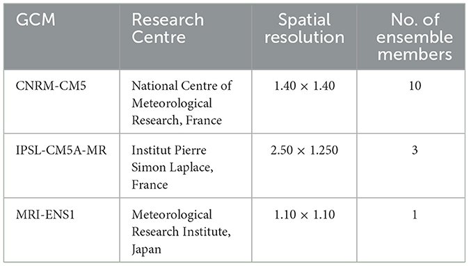
Table 1. Description related to three GCMs employed by the study.

Further, the observed gridded monthly precipitation and temperature variables for the historical period are obtained from the Indian Meteorological Department (IMD) (Rajeevan et al., 2006) over (1° × 1) spatial resolutions. Since there is a spatial resolution mismatch between the GCM outputs and the observed outputs, a bilinear interpolation is performed on the former to match with the observed grid resolution (1° × 1).

2.2. Bivariate asynchronous bias correction

The current study applies the Bivariate Asynchronous Bias Correction (BABC) approach, originally proposed by He et al. (2012), for bias correction of all the ensemble members from the three GCMs considered. The BABC approach is applied to develop an asynchronous predictand-predictor relationship between the monthly GCM and the monthly observed datasets for the historical period. The approach assigns bivariate ranks that generalize the concept of rankings for an univariate dataset, as proposed by Marden (2004). The authors understands that the proposed BABC can manage the non-stationary in the precipitation and temperature cross-correlation. The study considers that X represents two sets of GCM simulations (PRCP and Tavg/Tmax/Tmin), whereas Y represents two sets of the observed while considering the same pair of variables.

The GCMs and observed datasets are divided into X^train and Y^train, respectively, for model training. Two-thirds of the data are considered for training while the remaining GCM simulations, denoted as X^test, are considered for testing.

In the first step, all the datasets are univariately sorted in an ascending order and the univariate ranks are assigned. Following a univariate sorting, the marginal ranks are assigned next. For example, $R{X}_1^{train}(t)$ indicates the univariate rank related to the GCM response for the first variable, $X_1^{train}(t)$, where $X_1^{train}(t)$ is the first GCM variable at time step “t”. The marginal rank $M{X}_1^{train}(t)$ for $X_1^{train}(t)$ is estimated using Equation (1).

$\begin{array}{ll}{MX}_1^{train}(t)=\frac{R{X}_1^{train}(t)-0.5}{n}& (1)\end{array}$

Where n = the total number of observations in either the training or the testing dataset.

Bivariate ranks are applied on training datasets at different stages. For example, at stage K=1, the bivariate rank $P_t^{1,M{X}_1^{train}}$ for $M{X}_1^{train}(t)$ is calculated using Equation (2).

$\begin{array}{ll}\begin{array}{l}\begin{array}{l} P_t^{1,X_1^{train} }=\frac{4}{\text{π}n}{\displaystyle \sum _{i=1}^n}\\ \frac{M{X}_1^{train}(t)-M{X}_1^{train}(i)}{\sqrt{{\left[M{X}_1^{train}(t)-M{X}_1^{train}(i)\right]}^2+{\left[M{X}_2^{train}(t)-M{X}_2^{train}(i)\right]}^2}}\end{array}\hfill \end{array}& (2)\end{array}$

Similarly, the bivariate ranks for k=2 can be applied using Equation (3).

$\begin{array}{ll}\begin{array}{l}\begin{array}{l}{P}_t^{2,X_1^{train} }=\frac{4}{\text{π}n}{\displaystyle \sum _{i=1}^n}\\ \frac{P_t^{1,X_1^{train} }-P_i^{1,X_1^{train} }}{\sqrt{{\left[P_t^{1,X_1^{train} }-P_i^{1,X_1^{train} }\right]}^2+{\left[P_t^{1,X_2^{train} }-P_i^{1,X_2^{train} }\right]}^2}}\end{array}\hfill \end{array}& (3)\end{array}$

The current study repeats the process till k = 5, where $P_t^k$ denotes k^th as the consecutive transformation under the position function $P_t^{}$ for the same set of points. It is considered that as k increases, the distribution of $P_t^k$(X(t)) approaches a fixed stationary distribution regardless of the initial distribution of X (t), as long as X (t) is a continuous variable. Following the training, the bivariate ranks are applied on the GCM testing data and the same procedure is repeated for k = 5. The bivariate ranking equations for the testing period are shown for the first and second stages. Figure 1 demonstrates how the data points having non-circular distribution at the first stage shift to a stationary position after three transformations. The study does not find further changes in the distribution for the consecutive ranking stages.

$\begin{array}{ll}\begin{array}{l}\begin{array}{l}{P}_{t^{\prime }}^{1,X_1^{test} }=\frac{4}{\text{π}n}{\displaystyle \sum _{i=1}^n}\\ \frac{M{X}_1^{test}(t^{\prime })-M{X}_1^{train}(i)}{\sqrt{{\left[M{X}_1^{test}(t^{\prime })-M{X}_1^{train}(i)\right]}^2+{\left[M{X}_2^{test}(t^{\prime })-M{X}_2^{train}(i)\right]}^2}}\end{array}\hfill \end{array}& (4)\end{array}$

$\begin{array}{ll}\begin{array}{l}\begin{array}{l}{P}_{t^{\prime }}^{2,X_1^{test} }=\frac{4}{\text{π}n}{\displaystyle \sum _{i=1}^n}\\ \frac{P_{t^{\prime }}^{1,X_1^{test} }-P_i^{1,X_1^{train} }}{\sqrt{{\left[P_{t^{\prime }}^{1,X_1^{test} }-P_i^{1,X_1^{train} }\right]}^2+{\left[P_{t^{\prime }}^{2,X_1^{test} }-P_i^{2,X_1^{train} }\right]}^2}}\end{array}\hfill \end{array}& (5)\end{array}$

FIGURE 1

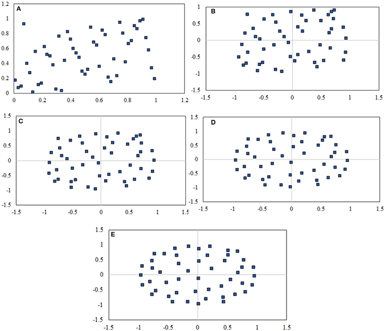
Figure 1. Different stages of bivariate ranking, where (A) marginal ranks, (B) bivariate ranks stage-1, (C) bivariate ranks stage-2, (D) bivariate ranks stage-4, (E) bivariate ranks stage-6.

In Equations (4) and (5), The marginal and bivariate ranks from the training datasets are considered as future GCM datasets which may not contain a complete set of ranks. The proposed approach assumes that, at a stationary stage of k = 5 during testing, the bivariate rankings from the GCM datasets matches that of the bias-corrected one, basically meaning $P_{}^{5,X_{}^{test}}=P_{}^{5,Y_{}^{test}}$. Hence, the objective is to find a suitable $Y^{BC}=[Y_1^{BC},Y_2^{BC}]$ that satisfies the previous equality. Toward this end, the minimizer of Equation 6 provides a new position of the GCM dataset depending on K.

$\begin{array}{l}L\left(Q\right)={\displaystyle \sum _{t=1}^n[{\left[P_t^{k,Y_1^{train}}-Q_1\right]}^2+{\left[P_t^{k,Y_2^{train}}-Q_2\right]}^2}\\ +\frac{\text{π}}{4}\left[\left[P_t^{k,Y_1^{train}}-Q_1\right]\right]P_{t^{\prime }}^{1,X_1^{tes{t}^2}}+\frac{\pi }{4}{\left[P_t^{k,Y_2^{train}}-Q_2\right]}^2{P}_{t^{\prime }}^{1,X_2^{test}}]& (6)\end{array}$

2.3. Asynchronous canonical correlation analysis

The current study considers another bivariate bias-correction approach—the Asynchronous Canonical Correlation Analysis (ACCA)—to compare the model's performance with BABC. ACCA, originally developed by Bhowmik et al. (2017), follows two major steps—(i) Bivariate sorting of the GCM and observed data based on the joint probability of the occurrence of precipitation and temperature, and (ii) Developing a predictor-predictand based Canonical Correlation Analysis (CCA) model using the sorted datasets. This approach assumes that bivariate sorting should ensure an asynchronous matching between the GCM and the observed variables, since both share the measurements that do not have a monthly correspondence, though the joint probabilities between the datasets matches. Further, the Canonical Correlation Analysis is considered as the apex among the regression techniques, with an ability to yield multivariable dependence. The ACCA was applied earlier to bias-correct meteorological variables over contiguous United States, but the approach is being applied to India for the first time. Additional details related to ACCA can be found in Bhowmik et al. (2017). The authors coded BABC and ACCA in MATLAB 2021a.

2.4. Performance evaluation

2.4.1. BABC vs. Raw GCM

BABC is applied separately on the bivariate pairs of PRCP-Tavg, PRCP-Tmax, and PRCP-Tmin from fourteen ensemble members from the three GCMs. However, only the performance evaluation related to the PRCP-Tavg is presented in while the results related to PRCP-Tmax and PRCP-Tmin are provided as Supplementary material. The performance of BABC is evaluated based on a fraction change metric (∅) which corresponds with the mean, the standard deviation, and the cross-correlation. The metric calculates the relative improvement in the statistical attributes achieved by the proposed bias-correction approach over their observed estimates.

$\begin{array}{llll}{\varnothing }_{mean}& =& \frac{{\mu }_{BC}-{\mu }_{Obs}}{{\mu }_{GCM}-{\mu }_{Obs}}& (7)\end{array}$

$\begin{array}{llll}{\varnothing }_{std}& =& \frac{{\sigma }_{BC}-{\sigma }_{Obs}}{{\sigma }_{GCM}-{\sigma }_{Obs}}& (8)\end{array}$

$\begin{array}{llll}{\varnothing }_{corr}& =& \frac{|\rho \left(PRC{P}_{BC},Tav{g}_{BC}\right)-\rho \left(PRC{P}_{Obs},Tav{g}_{Obs}\right)|}{|\rho \left(PRC{P}_{GCM},Tav{g}_{GCM}\right)-\rho \left(PRC{P}_{Obs},Tav{g}_{Obs}\right)|}& (9)\end{array}$

Where u is the mean, σ is the standard deviation, and ρ is the cross-correlation. Subscripts BC, obs, GCM indicate the bias-corrected, observed, and raw GCM data, respectively. ∅_mean and ∅_std are estimated for the four variables. A fraction change value related to the mean or the standard deviation between −1and 1 (>1 and <-1) indicates that the bias has reduced (increased) following the application of BABC. The metric is slightly revised to estimate the bias in the cross-correlation. A fraction change in the cross-correlation between 0 and 1 (>1) confirms that the bias in the correlation has reduced (increased) in the bias-corrected outputs.

2.4.2. BABC vs. ACCA

In the final analysis, the study compares the performance of the BABC with another bivariate bias-correction approach—ACCA. Toward this, the fraction change equations suggested in Subsection 2.4.2 are slightly modified (Equations 10–12). However, the interpretation of the fraction change metric remains the same. A value of ∅_mean and ∅_Std within −1 to 1 indicates that the BABC lesser bias in the mean and the standard deviation as compared to ACCA. On the other hand, a value of ∅_corr higher than 1 indicates that the ACCA performs better than the BABC in reducing bias in the cross-correlation.

$\begin{array}{llll}{\varnothing }_{mean}& =& \frac{{\mu }_{OBS}-{\mu }_{BABC}}{{\mu }_{OBS}-{\mu }_{ACCA}}& (10)\end{array}$

$\begin{array}{llll}{\varnothing }_{std}& =& \frac{{\sigma }_{OBS}-{\sigma }_{BABC}}{{\sigma }_{OBS}-{\sigma }_{ACCA}}& (11)\end{array}$

$\begin{array}{llll}{\varnothing }_{corr}& =& \frac{|\rho \left(PRC{P}_{OBS},Tav{g}_{OBS}\right)-\rho \left(PRC{P}_{BABC},Tav{g}_{BABC}\right)|}{|\rho \left(PRC{P}_{OBS},Tav{g}_{OBS}\right)-\rho \left(PRC{P}_{ACCA},Tav{g}_{ACCA}\right)|}& (12)\end{array}$

3. Results

3.1. Observed cross-correlation

The cross-correlation between the observed precipitation (PRCP) and the observed temperature (Tavg) is estimated for each grid point to understand the spatial variation in cross-correlation over India. Figure 2 presents the observed cross-correlation for 4 months (January, March, July, and November), each representing the four seasons. The grid points where the observed cross-correlation is statistically significant are marked with a circle. The statistical significance at 95% confidence level in the cross-correlation is determined based on [±1.96/√(n−3)], where n is the number of observations. For the current study, if a cross-correlation is higher or lesser than ±0.289, the corresponding grid point is considered statistically significant. Results related to PRCP-Tmax and PRCP-Tmin are presented in the Supplementary Figures 1A, B. Additionally, spatially averaged cross-correlations between observed monthly precipitation (PRCP) and monthly temperature (Tavg) across six climate homogeneous regions are presented in Supplementary Figure 2. These regions were suggested by the Indian Meteorological Department.

FIGURE 2

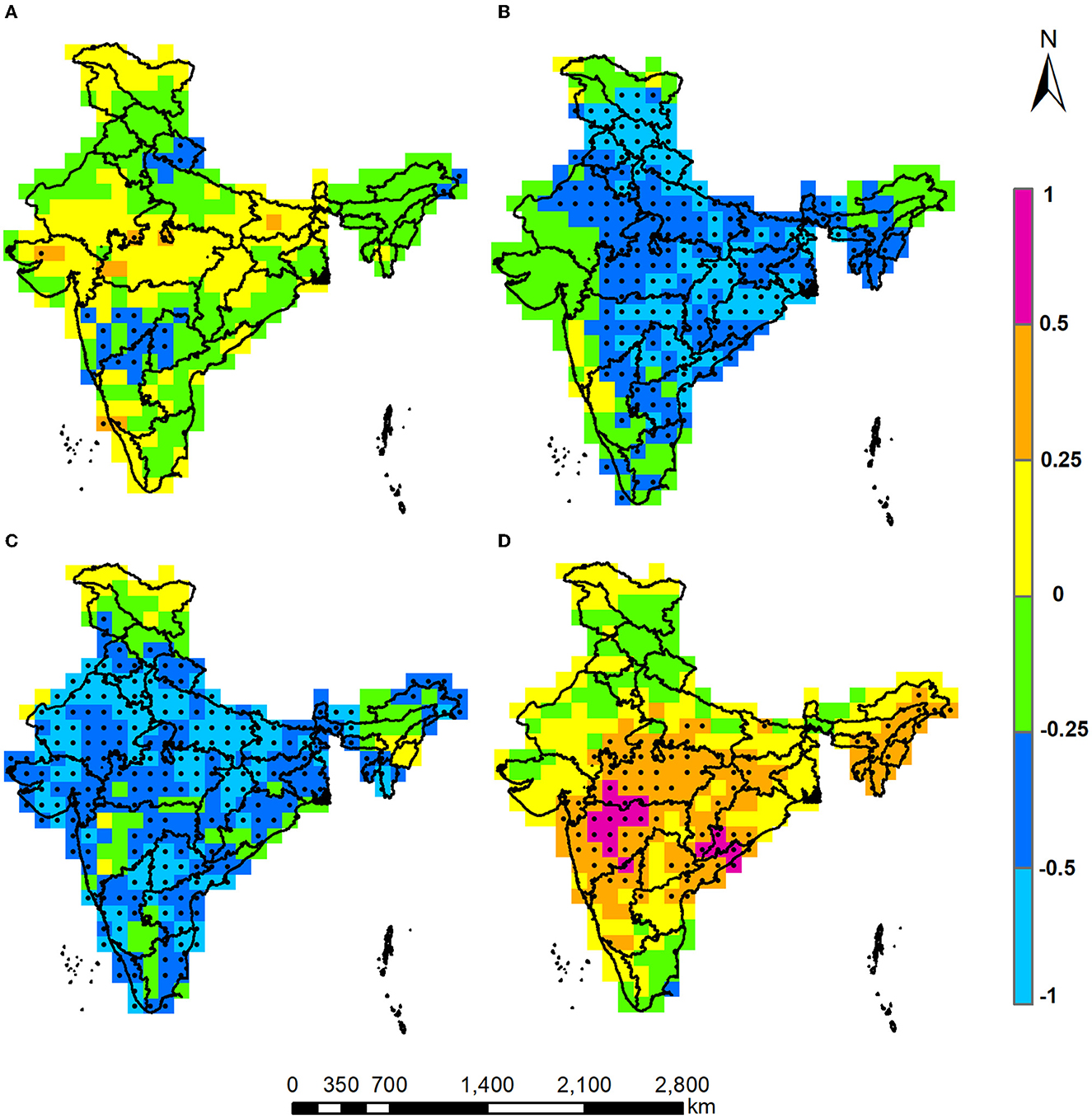
Figure 2. Cross-Correlation between observed monthly precipitation (PRCP) and monthly average temperature (Tavg) for historical time-frame 1951–1999. Marked grids points are indicating the statistical significance at 95% confidence level for the months of January (A), March (B), July (C), and November (D).

Figure 2A shows that cross-correlation between the observed PRCP and the observed Tavg during January is positive but statistically insignificant. However, during November, the variables are positively correlated, except for a few regions of Northern (and Southeast) India (Figure 2D). Further, during March and July, most of the grids exhibit a negative cross-correlation with values between −0.25 and −0.5. The negative cross-correlations during March and July also exhibit statistical significance. From Supplementary Figures 1, 2, The study found that the PRCP and the Tmax (PRCP and Tmin) show a strong dependence during the pre-monsoon season (post-monsoon). Overall, the study found that a strong negative cross-correlation exists between the observed precipitation and observed temperature during the monsoon months, indicating the role of rainfall in providing relief from the heat accumulated during the summer/ pre-monsoon months (Das Bhowmik et al., 2020). During winter, a positive cross-correlation between the PRCP and Tavg is observed for Central and South-Central India, indicating that a rainfall during the winter results in an increase in temperature. Overall, the dependencies between precipitation and temperature exhibit substantial spatio-temporal variation resulting from the northeast and southwest monsoonal circulations, which should be considered a major statistical attribute during the bias-correction of GCM outputs.

3.2. BABC vs. Raw GCM analysis

Figure 3 presents the performance of BABC in reducing the bias in mean, standard deviation, and cross-correlation. At each grid point, the study estimated the fraction change in mean (∅_mean), standard deviation (∅_SD), and cross-correlation (∅_corr) as defined in Equations (7)–(9). The fraction change metric is estimated for fourteen ensembles and the ensemble average of the metric is plotted. The results related to PRCP and Tavg for 4 months are presented in Figure 3 while the results related to the Tmax and Tmin are presented as Supplementary Figure 3. At each grid point, the study measures the metric for fourteen ensembles and plots the ensemble average estimate of the metric. In addition, spatially averaged fraction change in cross-correlation (PRCP-Tavg) estimates across six climate homogeneous regions are presented in the Supplementary Figure 4. The study found that BABC performs satisfactorily in reducing the bias in the mean and the standard deviation over India; however, its performance varies across months and regions. The proposed approach performs better at reducing the bias in the mean and the standard deviation during the monsoonal month (July) as compared to the other months. The proposed approach exhibits superior performance in reducing the bias in the mean of the Tavg as compared to the bias in the mean of the PRCP. Additionally, the approach performs better at reducing the bias in the standard deviation in Tavg as compared to the same in PRCP. The authors note that the raw GCMs have higher bias in their PRCP than the Tavg. Also, the raw GCM outputs could efficiently yield the inter-seasonal variation in the monthly temperature (Salvi et al., 2011). Regarding the bias in cross-correlation, as shown in Figures 3Q–T, the results are mixed since the proposed approach typically performs better in non-monsoonal months as compared to the monsoonal months. During July, the raw GCM cross-correlation exhibits a lower bias as compared to the bias-corrected outputs. However, BABC successfully reduces the bias in cross-correlation during November, a non-monsoon month. A comprehensive analysis related to the performance of the BABC in reducing the bias in cross-correlation is provided in Table 2 and additional information is presented in the Supplementary Tables 1, 2. Monsoon months in India typically experiences a strong negative cross-correlation between precipitation and temperature. Meteorological factors other than precipitation (for example wind, relative humidity) have lesser influence on the heat accumulated during summer compared to the influence of precipitation on the accumulated heat. Although there is a long-standing debate on the efficiency of GCMs in simulating the spatio-temporal characteristics of monsoon (Anand et al., 2018), the strong negative P-T correlation during monsoon is typically well-captured by raw GCM outputs (see Supplementary Figure 5). Following a bias-correction, the bias in the mean and in the standard deviation improve; however, as a trade-off, the slight bias in the P-T cross-correlation gets impacted in the bias-corrected outputs. In contrast, the bias in the cross-correlation for raw GCM outputs is higher during non-monsoonal months as compared to monsoon months, therefore, BABC performs better in reducing the bias in the cross-correlation during non-monsoonal months as compared to monsoon months.

FIGURE 3

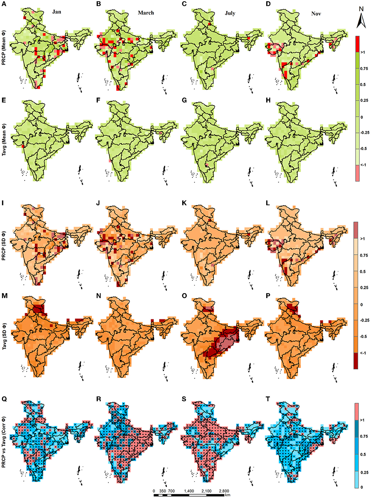
Figure 3. Maps show fraction change in the mean (∅_mean), standard deviation (∅_SD), and cross-correlation (∅_corr) while compared between the bias-corrected (using BABC) and the observed datasets for the months January (A, E, I, M, Q); March (B, F, J, N, R), July (C, G, K, O, S); and November (D, H, L, P, T). Grid points showing statistically significant observed cross-correlation (Q–T) are indicated as a black circle.

TABLE 2

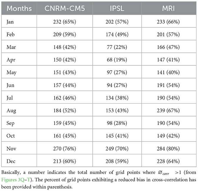
Table 2. Table presents the total number of grid points where the bias in the cross-correlation has been reduced following the application of BABC.

3.3. Reproduction of bias-corrected precipitation time-series

The current study applies bivariate bias-correction separately the for PRCP-Tavg, PRCP-Tmax, and PRCP-Tmin. Therefore, any ensemble member of precipitation over a particular grid point receives three bias-corrected time-series. Since the bivariate bias-correction yields the observed cross-correlation between the precipitation and the temperature variable, the three bias-corrected precipitation time-series might differ slightly in their monthly values, but the three-precipitation series should maintain an overall monthly correspondence. To ensure the reproduction of the bias-corrected precipitation series, the study plotted three bias-corrected precipitation time-series from a randomly selected grid point (Figure 4). The study found that the high and low precipitation months show good correspondence between the three bias-corrected precipitation series. Additionally, the correlation between any two of the precipitation series is higher than 0.9. Therefore, the study concludes that the proposed approach has reproducibility when applied on different combinations of the raw GCM variables.

FIGURE 4

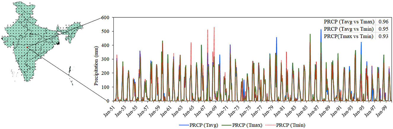
Figure 4. Three time series of bias-corrected precipitation while paired with three temperature variables (Tavg, Tmax, Tmin) at a selected grid point.

3.4. Simulation of precipitation and temperature seasonality

In the current subsection, the study investigates the efficiency of the BABC approach in yielding the seasonality in PRCP and Tavg over India. Toward this end, the long-term mean of the observed time series, the raw GCM outputs, and the bias-corrected GCM outputs are estimated. The raw ensemble members from the CNRM-CM5 have similar values. Therefore, only one ensemble member from the CNRM-CM5 is considered. On the other hand, for the two remaining GCMs, ensemble averaging is not performed due to which the results show inter-ensemble variations. Figures 5, 6 presents the long-term mean in precipitation from the observed and the raw GCM (bias-corrected GCM) outputs. All the three GCMs fail to yield PRCP seasonality; however, the CNRM-CM5 performs slightly better than the MRI and IPSL. Correspondingly, following bias-correction, precipitation seasonality is accurately represented by all the five ensemble members from the three GCMs. Following the seasonality analysis in PRCP, tavg seasonality is examined for post-monsoon and pre-monsoon seasons. as India experiences significant hot and humid weather during these two seasons. Figures 7, 8 presents the long-term mean in Tavg from the observed and raw GCM (bias-corrected GCM) outputs for 6 months. All the three GCMs fail to yield the high pre-monsoon temperature. On the other hand, in the post-monsoon season, the MRI and IPSL perform slightly better than the CNRM-CM5. Overall, none of the GCMs successfully simulate Tavg seasonality. However, the performance of the GCMs substantially improves following bias correction (Figure 8). The low inter-annual variation in Tavg exhibited by the raw GCMs is corrected by the proposed BABC approach. Similar performance of the raw GCM outputs and bias-corrected outputs can be found for Tmax seasonality and Tmin seasonality. The results are presented in Supplementary Figures 6–9. A comparison between Figures 6, 8 indicates that GCMs are more uncertain in simulating the mean precipitation than the mean temperature which potentially resulted from the higher spatial variation in the observed precipitation as compared to the observed temperature. Overall, the study concludes that BABC successfully captures seasonality in PRCP and Tavg by yielding inter-seasonal variations in the meteorological variables.

FIGURE 5

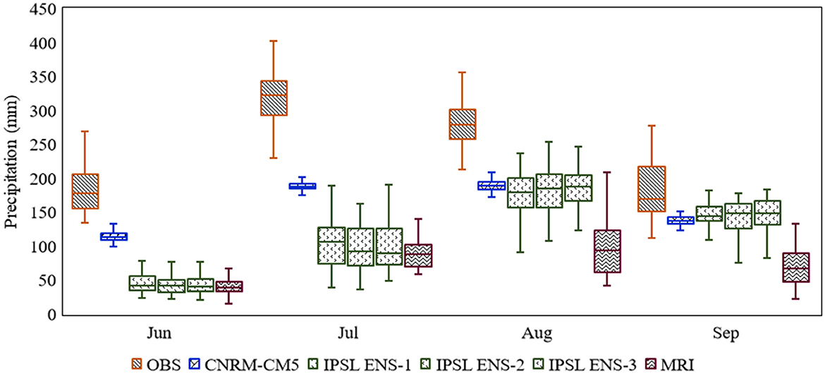
Figure 5. Box plots show the long-term average precipitation for four monsoon months from five Raw GCM ensemble members and from the observed. The spread of a box plot represents the spatial variation in the average PRCP across grid points. One ensemble member is selected for CNRM-CM5 and MRI; whereas, all three members are selected for the IPSL ensemble.

FIGURE 6

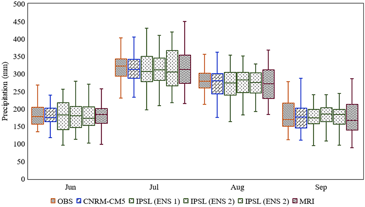
Figure 6. Box plots show the long-term average precipitation for four monsoonal months from five bias-corrected (using BABC) GCM ensemble members and the observed. Rest is same in Figure 5.

FIGURE 7

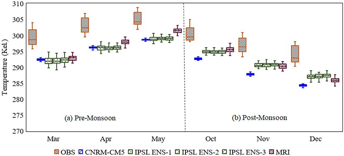
Figure 7. Box plots show the long-term mean Tavg for six pre-monsoon (A) and post-monsoon (B) months from five raw GCM ensemble members and the observed. Rest is same as Figures 5, 6.

FIGURE 8

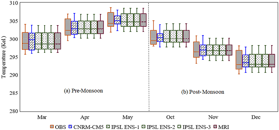
Figure 8. Box plots show the long-term mean Tavg for six pre-monsoon (A) and post-monsoon (B) months from five bias-corrected (using BABC) GCM ensemble members and the observed. Rest is the same as Figures 5–7.

3.5. BABC vs. ACCA analysis

The performance comparison between BABC against ACCA is carried out using the statistical metrics suggested in Equations (10)–(12). Similar to Subsection 3.2, fraction change metrics are processed across ensemble members. Figure 9 presents the results related to PRCP and Tavg for 4 months; additional results related to Tmax and Tmin are presented as Supplementary Figure 10. Further, spatially averaged fraction change in cross-correlation (PRCP-Tavg) estimates across six climate homogeneous regions are presented in the Supplementary Figure 11. BABC performs significantly better than ACCA in reducing the bias in standard deviation of PRCP. During March and July, the performance of BABC is slightly better than ACCA in reducing the bias in the standard deviation of Tavg. Further, the study found, the bias in the cross-correlation during July could be reduced further by BABC as compared to the ACCA. The performance trade-off of the ACCA in yielding the mean and standard deviation results in influencing the joint dependence between PRCP and Tavg. A comprehensive analysis related to the performance of BABC in reducing bias in the cross-correlation as compared to the ACCA is provided in Table 3. An almost similar performance comparison between the BABC and the ACCA can be observed when Tmax and Tmin are considered (see Supplementary Figure 10). To note that the difference between ACCA and univariate bias correction has already been performed in one of our previous studies (Bhowmik et al., 2017). Hence, the current study refrains from comparing BABC with a univariate bias-correction.

TABLE 3

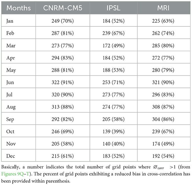
Table 3. Table presents the total number of grid points where the bias in the cross-correlation has been reduced following the application of BABC vs. ACCA.

FIGURE 9

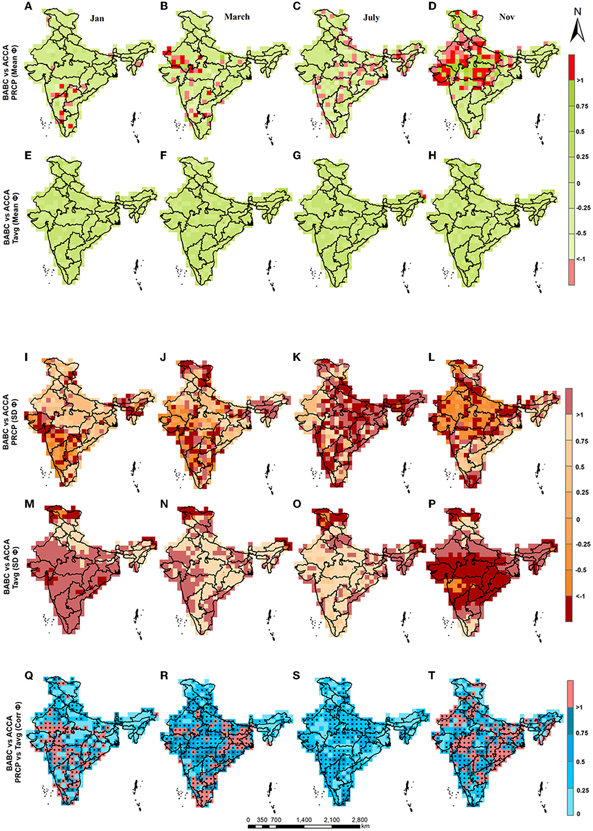
Figure 9. Maps show fraction change in the mean (∅_mean), standard deviation (∅_SD), and cross-correlation (∅_corr) while compared between the two bias-corrected (BABC vs ACCA) datasets for the months January (A, E, I, M, Q); March (B, F, J, N, R), July (C, G, K, O, S); and November (D, H, L, P, T). Grid points showing statistically significant observed cross-correlation (Q, R, S, T) are indicated as a black circle.

4. Summary and discussion

The current study employed a bivariate bias correction approach to post-process GCM ensembles over India. The bias-correction approach relies on a bivariate ranking scheme that finds a stationary distribution of the asynchronous measurements. The study compares the bias corrected outputs with the raw GCM dataset as well as with the outputs from another bivariate approach: ACCA focusing in yielding the observed cross correlation between rainfall and temperature. Additionally, the study also focuses on reproducing the seasonal attributes of Indian precipitation and temperature in the bias-corrected outputs. The major findings of the current study are as follows:

1. The study found that, typically, a negative cross-correlation between the observed monthly PRCP and the observed monthly Tavg exists in India.

2. The BABC approach successfully reduces bias in the mean and in the standard deviation of the PRCP and Tavg. However, it performs better in reducing bias in the cross-correlation during the non-monsoonal months as compared to the monsoonal months.

3. The study confirmed that precipitation time series can be reproduced following bias-correction, irrespective of either of the three temperature variables being considered as the second variable in the ranking scheme.

4. The BABC successfully reproduces precipitation climatology for the monsoon months. Also, the approach yields temperature climatology for the pre- and post- monsoon seasons that experience high inter-seasonal variations in temperature.

5. Finally, the study reports that the BABC and the ACCA both perform equally well in reducing bias in the standard deviation and the mean. However, the BABC performs better than the ACCA in reducing bias in the cross-correlation.

A major limitation related to the application of bivariate bias-correction is that it takes a significant amount of computation time when the bias-correction is applied at a regional scale. The computation time is further increased when optimization is performed at the grid points for the monthly models. The computation time can increase further if finer resolution datasets are considered. The application requires a high-performance cluster computing facility, which shall be considered in the near future to estimate changes in the cross-correlation resulting from anthropogenic climate change. The current study considered the algorithm suggested by Campbell et al. (2011) to find the minimizer of Equation (6). However, He et al. (2012) found that it is better to consider Newton-Raphson as a degeneracy condition (originally suggested by Chaudhuri, 1996) is necessary but not a sufficient condition to check whether the optimized solution is an element of the observed variable.

Former studies have concluded that bivariate bias-correction could not yield the observed cross-correlation in bias-corrected products (Cannon, 2016, 2018; Bhowmik et al., 2017; Vrac, 2018; Eum et al., 2020). The limitation to yield the observed cross-correlation can be a potential problem for bias-correction as it may result in errors in the hydrologic simulations with the univariate bias-corrected outputs (Salvi and Ghosh, 2013; Bhowmik et al., 2017; Seo et al., 2019). Therefore, the development of bivariate approaches is essential as the P-T dependence is expected to be influenced by the increase in greenhouse gas concentrations in the near future. The application of bivariate bias-correction on future GCM projections would help researchers to quantify the potential change in P-T dependence. The authors note that the current study considered a linear relationship between P-T, although it is traditionally considered to follow a non-linear relationship: Clausius Clapeyron equation. The advantage of the BABC is that it does not consider any functional form of the P-T dependence; hence, a non-linear dependence can also be yielded by the proposed approach.

The current study applied BABC and ACCA approaches to bias-correct monthly meteorological variables. The same approaches can also be applied to the daily or sub-daily meteorological series. However, the authors note that the application of BABC at a daily temporal resolution would further increase the computation requirements. Additionally, precipitation and temperature dependence are best witnessed at a monthly scale since several local scale features such as wind, relative humidity, and geomorphic characteristics have a higher influence on the daily precipitation as compared to the temperature (Dingman, 2015). The current study has performed bias-correction for 4 months: January, March, July, and November. Considering the considerable computation time required to perform the bias-correction, we decided to run the bias-correction for only 4 months with the expectation that similar performance can be witnessed for other months within a season. Further, the daily statistical attributes (for example, day-to-day variation) of meteorological variables need to be considered if the BABC is applied at a daily scale. Considering these issues, the current study suggests that the application of a bivariate bias-correction is appropriate in the case of a hydrological long-term simulation being performed at a monthly scale. Overall, the study found that, historically, precipitation and temperature are strongly associated at a monthly scale, and the proposed bivariate bias-correction successfully yields the observed cross-correlation in the GCM outputs.

Data availability statement

The original contributions presented in the study are included in the article/Supplementary material, further inquiries can be directed to the corresponding author.

Author contributions

CG performed investigation, methodology, visualization, data collection, analysis of findings, software, and writing the original draft. RB performed investigation, methodology, visualization, analysis of findings, funding acquisition, validation, supervision, writing, and reviewing and editing the draft. The authors are significantly contributed to the present study. The authors have read and approved the final manuscript.

Funding

This research was funded by an INSPIRE Faculty Fellowship (IFA-18-ENG262) from the Department of Science and Technology, Govt. of India, received by RB.

Acknowledgments

The authors would like to acknowledge the Indian Metrological Department (IMD) for providing the precipitation and temperature datasets and the World Climate Research Program (WCRP—powered by ESGF https://esgf-node.llnl.gov/search/cmip5/) for providing the GCMs datasets from different models and different ensemble members.

Conflict of interest

The authors declare that the research was conducted in the absence of any commercial or financial relationships that could be construed as a potential conflict of interest.

Publisher's note

All claims expressed in this article are solely those of the authors and do not necessarily represent those of their affiliated organizations, or those of the publisher, the editors and the reviewers. Any product that may be evaluated in this article, or claim that may be made by its manufacturer, is not guaranteed or endorsed by the publisher.

Supplementary material

The Supplementary Material for this article can be found online at: https://www.frontiersin.org/articles/10.3389/fclim.2023.1067960/full#supplementary-material

References

Abatzoglou, J. T., and Brown, T. J. (2012). A comparison of statistical downscaling methods suited for wildfire applications. Int. J. Climatol. 32, 772–780. doi: 10.1002/joc.2312

CrossRef Full Text | Google Scholar

Anand, A., Mishra, S. K., Sahany, S., Bhowmick, M., Rawat, J. S., and Dash, S. K. (2018). Indian summer monsoon simulations: usefulness of increasing horizontal resolution, manual tuning, and semi-automatic tuning in reducing present-day model biases. Sci. Rep. 8, 1–15. doi: 10.1038/s41598-018-21865-1

PubMed Abstract | CrossRef Full Text | Google Scholar

Ayar, P. V., Vrac, M., and Mailhot, A. (2021). Ensemble bias correction of climate simulations: preserving internal variability. Sci. Rep. 11, 1–9. doi: 10.1038/s41598-021-82715-1

PubMed Abstract | CrossRef Full Text | Google Scholar

Baño-Medina, J., Manzanas, R., and Gutiérrez, J. M. (2020). Configuration and intercomparison of deep learning neural models for statistical downscaling. Geosci. Model Dev. 13, 2109–2124. doi: 10.5194/gmd-13-2109-2020

CrossRef Full Text | Google Scholar

Bhowmik, R. D., Sankarasubramanian, A., Sinha, T., Patskoski, J., Mahinthakumar, G., and Kunkel, K. E. (2017). Multivariate downscaling approach preserving cross correlations across climate variables for projecting hydrologic fluxes. J. Hydrometeorol. 18, 2187–2205. doi: 10.1175/JHM-D-16-0160.1

CrossRef Full Text | Google Scholar

Bisht, D. S., Mohite, A. R., Jena, P. P., Khatun, A., Chatterjee, C., Raghuwanshi, N. S., et al. (2020). Impact of climate change on streamflow regime of a large Indian river basin using a novel monthly hybrid bias correction technique and a conceptual modeling framework. J. Hydrol. 590, 125448. doi: 10.1016/j.jhydrol.2020.125448

CrossRef Full Text | Google Scholar

Campbell, J. D., Taylor, M. A., Stephenson, T. S., Watson, R. A., and Whyte, F. S. (2011). Future climate of the Caribbean from a regional climate model. Int. J. Climatol. 31, 1866–1878. doi: 10.1002/joc.2200

CrossRef Full Text | Google Scholar

Cannon, A. J. (2016). Multivariate bias correction of climate model output: Matching marginal distributions and intervariable dependence structure. J. Clim. 29, 7045–7064. doi: 10.1175/JCLI-D-15-0679.1

CrossRef Full Text | Google Scholar

Cannon, A. J. (2018). Multivariate quantile mapping bias correction: an N-dimensional probability density function transform for climate model simulations of multiple variables. Clim. Dyn. 50, 31–49. doi: 10.1007/s00382-017-3580-6

CrossRef Full Text | Google Scholar

Chaudhuri, P. (1996). On a geometric notion of quantiles for multivariate data. J. Am. Stat. Assoc. 91, 862–872. doi: 10.1080/01621459.1996.10476954

PubMed Abstract | CrossRef Full Text | Google Scholar

Chen, J., Li, C., Brissette, F. P., Chen, H., Wang, M., and Essou, G. R. (2018). Impacts of correcting the inter-variable correlation of climate model outputs on hydrological modeling. J. Hydrol. 560, 326–341. doi: 10.1016/j.jhydrol.2018.03.040

CrossRef Full Text | Google Scholar

Das Bhowmik, R., Ng, T. L., and Wang, J. (2020). Understanding the impact of observation data uncertainty on probabilistic streamflow forecasts using a dynamic hierarchical model. Water Resour. Res. 56, e2019. doi: 10.1029/2019WR025463

CrossRef Full Text | Google Scholar

Das Bhowmik, R., Seo, S. B., and Sahoo, S. (2018). Streamflow simulation using bayesian regression with multivariate linear spline to estimate future changes. Water 10, 875. doi: 10.3390/w10070875

CrossRef Full Text | Google Scholar

Dingman, S. L. (2015). Physical Hydrology. Waveland Press.

Google Scholar

Dufresne, J. L., Foujols, M. A., Denvil, S., Caubel, A., Marti, O., and Aumont, O. (2013). Climate change projections using the IPSL-CM5 Earth System Model: from CMIP3 to CMIP5. Clim. Dyn. 40, 2123–2165. doi: 10.1007/s00382-012-1636-1

CrossRef Full Text | Google Scholar

Eum, H. I., Gupta, A., and Dibike, Y. (2020). Effects of univariate and multivariate statistical downscaling methods on climatic and hydrologic indicators for Alberta, Canada. J. Hydrol. 588, 125065. doi: 10.1016/j.jhydrol.2020.125065

CrossRef Full Text | Google Scholar

Gadgil, S. (2003). The Indian monsoon and its variability. Annu. Rev. Earth Planet. Sci. 31, 429–467. doi: 10.1146/annurev.earth.31.100901.141251

CrossRef Full Text | Google Scholar

Ghosh, S., and Mujumdar, P. P. (2006). Future rainfall scenario over Orissa with GCM projections by statistical downscaling. Curr. Sci. 90, 396–404.

Google Scholar

Ghosh, S., and Mujumdar, P. P. (2007). Nonparametric methods for modeling GCM and scenario uncertainty in drought assessment. Water Resour. Res. 43. doi: 10.1029/2006WR005351

CrossRef Full Text | Google Scholar

Ghosh, S., and Mujumdar, P. P. (2008). Statistical downscaling of GCM simulations to streamflow using relevance vector machine. Adv. Water Resour. 31, 132–146. doi: 10.1016/j.advwatres.2007.07.005

CrossRef Full Text | Google Scholar

Ghosh, S., Vittal, H., Sharma, T., Karmakar, S., Kasiviswanathan, K. S, Dhanesh, Y., et al. (2016). Indian summer monsoon rainfall: implications of contrasting trends in the spatial variability of means and extremes. PLoS ONE 11, e0158670. doi: 10.1371/journal.pone.0158670

PubMed Abstract | CrossRef Full Text | Google Scholar

Graham, L. P., Andréasson, J., and Carlsson, B. (2007). Assessing climate change impacts on hydrology from an ensemble of regional climate models, model scales and linking methods–a case study on the Lule River basin. Clim. Change 81, 293–307. doi: 10.1007/s10584-006-9215-2

CrossRef Full Text | Google Scholar

Hakala, K., Addor, N., and Seibert, J. (2018). Hydrological modeling to evaluate climate model simulations and their bias correction. J. Hydrometeorol. 19, 1321–1337. doi: 10.1175/JHM-D-17-0189.1

CrossRef Full Text | Google Scholar

He, X., Yang, Y., and Zhang, J. (2012). Bivariate downscaling with asynchronous measurements. J. Agric. Biol. Environ. Stat. 17, 476–489. doi: 10.1007/s13253-012-0098-6

CrossRef Full Text | Google Scholar

Hovenga, P. A., Wang, D., Medeiros, S. C., Hagen, S. C., and Alizad, K. (2016). The response of runoff and sediment loading in the Apalachicola River, Florida to climate and land use land cover change. Earths Fut. 4, 124–142. doi: 10.1002/2015EF000348

CrossRef Full Text | Google Scholar

Jarraud, M., and Steiner, A. (2014). Summary for policymakers, Managing the Risks of Extreme Events and Disasters to Advance Climate Change Adaptation: Special Report of the Intergovernmental Panel on Climate Change. Cambridge University Press.

Google Scholar

Li, F., Zhang, Y., Xu, Z., Teng, J., Liu, C., Liu, W., et al. (2013). The impact of climate change on runoff in the southeastern Tibetan Plateau. J. Hydrol. 505, 188–201. doi: 10.1016/j.jhydrol.2013.09.052

CrossRef Full Text | Google Scholar

Li, W., Sankarasubramanian, A., Ranjithan, R. S., and Brill, E. D. (2014). Improved regional water management utilizing climate forecasts: an interbasin transfer model with a risk management framework. Water Resour. Res. 50, 6810–6827. doi: 10.1002/2013WR015248

CrossRef Full Text | Google Scholar

Mallya, G., Mishra, V., Niyogi, D., Tripathi, S., and Govindaraju, R. S. (2016). Trends and variability of droughts over the Indian monsoon region. Weather Clim. Extremes 12, 43–68. doi: 10.1016/j.wace.2016.01.002

CrossRef Full Text | Google Scholar

Maraun, D. (2016). Bias correcting climate change simulations-a critical review. Curr. Clim. Change Rep. 2, 211–220. doi: 10.1007/s40641-016-0050-x

CrossRef Full Text | Google Scholar

Maraun, D., Wetterhall, F., Ireson, A. M., Chandler, R. E., Kendon, E. J., Widmann, M., et al. (2010). Precipitation downscaling under climate change: recent developments to bridge the gap between dynamical models and the end user. Rev. Geophys. 48. doi: 10.1029/2009RG000314

CrossRef Full Text | Google Scholar

Marden, J. I. (2004). Positions and QQ plots. Stat. Sci. 19, 606–614. doi: 10.1214/088342304000000512

CrossRef Full Text | Google Scholar

Piani, C., Haerter, J. O., and Coppola, E. (2010). Statistical bias correction for daily precipitation in regional climate models over Europe. Theoret. Appl. Climatol. 99, 187–192. doi: 10.1007/s00704-009-0134-9

CrossRef Full Text | Google Scholar

Pierce, D. W., Cayan, D. R., Maurer, E. P., Abatzoglou, J. T., and Hegewisch, K. C. (2015). Improved bias correction techniques for hydrological simulations of climate change. J. Hydrometeorol. 16, 2421–2442. doi: 10.1175/JHM-D-14-0236.1

CrossRef Full Text | Google Scholar

Pierce, D. W., Cayan, D. R., and Thrasher, B. L. (2014). Statistical downscaling using localized constructed analogs (LOCA). J. Hydrometeorol. 15, 2558–2585. doi: 10.1175/JHM-D-14-0082.1

CrossRef Full Text | Google Scholar

Prasanna, V. (2018). Statistical bias correction method applied on CMIP5 datasets over the Indian region during the summer monsoon season for climate change applications. Theoret. Appl. Climatol. 131, 471–488. doi: 10.1007/s00704-016-1974-8

CrossRef Full Text | Google Scholar

Rajeevan, M., Bhate, J., Kale, J. D., and Lal, B. (2006). High resolution daily gridded rainfall data for the Indian region: analysis of break and active monsoon spells. Curr. Sci. 296–306.

Google Scholar

Ruelland, D., Ardoin-Bardin, S., Collet, L., and Roucou, P. (2012). Simulating future trends in hydrological regime of a large Sudano-Sahelian catchment under climate change. J. Hydrol. 424, 207–216. doi: 10.1016/j.jhydrol.2012.01.002

CrossRef Full Text | Google Scholar

Salvi, K., and Ghosh, S. (2013). High-resolution multisite daily rainfall projections in India with statistical downscaling for climate change impacts assessment. J. Geophys. Res. Atmosph. 118, 3557–3578. doi: 10.1002/jgrd.50280

CrossRef Full Text | Google Scholar

Salvi, K., Kannan, S., and Ghosh, S. (2011). “Statistical downscaling and bias-correction for projections of Indian rainfall and temperature in climate change studies,” in 4th International Conference on Environmental and Computer Science, 16–18.

Google Scholar

Seo, S. B., Bhowmik, R. D., Sankarasubramanian, A., Mahinthakumar, G., and Kumar, M. (2019). The role of cross-correlation between precipitation and temperature in basin-scale simulations of hydrologic variables. J. Hydrol. 570, 304–314. doi: 10.1016/j.jhydrol.2018.12.076

CrossRef Full Text | Google Scholar

Seo, S. B., and Kim, Y.-O. (2018). Impact of spatial aggregation level of climate indicators on a national-level selection for representative climate change scenarios. Sustainability 10, 2409. doi: 10.3390/su10072409

CrossRef Full Text | Google Scholar

Sharma, D., Das Gupta, A., and Babel, M. S. (2007). Spatial disaggregation of bias-corrected GCM precipitation for improved hydrologic simulation: Ping River Basin, Thailand. Hydrol. Earth Syst. Sci. 11, 1373–1390. doi: 10.5194/hess-11-1373-2007

CrossRef Full Text | Google Scholar

Sharma, S., and Mujumdar, P. (2017). Increasing frequency and spatial extent of concurrent meteorological droughts and heatwaves in India. Sci. Rep. 7, 1–9. doi: 10.1038/s41598-017-15896-3

PubMed Abstract | CrossRef Full Text | Google Scholar

Singh, R. K., Sinha, V. S. P., Joshi, P. K., and Kumar, M. (2000). Land Use, Land-Use Change and Forestry: A Special Report of the Intergovernmental Panel on Climate Change. Cambridge University Press.

PubMed Abstract | Google Scholar

Smitha, P. S., Narasimhan, B., Sudheer, K. P., and Annamalai, H. (2018). An improved bias correction method of daily rainfall data using a sliding window technique for climate change impact assessment. J. Hydrol. 556, 100–118. doi: 10.1016/j.jhydrol.2017.11.010

CrossRef Full Text | Google Scholar

Subrahmanyam, K. V., and Kumar, K. K. (2013). CloudSat observations of cloud-type distribution over the Indian summer monsoon region. Ann. Geophys. Copernic. GmbH 1155–1162. doi: 10.5194/angeo-31-1155-2013

CrossRef Full Text | Google Scholar

Tan, Y., Guzman, S. M., Dong, Z., and Tan, L. (2020). Selection of effective GCM bias correction methods and evaluation of hydrological response under future climate scenarios. Climate 8, 108. doi: 10.3390/cli8100108

CrossRef Full Text | Google Scholar

Taylor, K. E., Stouffer, R. J., and Meehl, G. A. (2012). An overview of CMIP5 and the experiment design. Bull. Am. Meteorol. Soc. 93, 485–498. doi: 10.1175/BAMS-D-11-00094.1

PubMed Abstract | CrossRef Full Text | Google Scholar

Teutschbein, C., and Seibert, J. (2013). Is bias correction of regional climate model (RCM) simulations possible for non-stationary conditions? Hydrol. Earth Syst. Sci. 17, 5061–5077. doi: 10.5194/hess-17-5061-2013

CrossRef Full Text | Google Scholar

Trenberth, K. E., and Shea, D. J. (2005). Relationships between precipitation and surface temperature. Geophys. Res. Lett. 32. doi: 10.1029/2005GL022760

CrossRef Full Text | Google Scholar

Ullah, S., You, Q., Zhang, Y., Bhatti, A. S., Ullah, W., Hagan, D. F. T., et al. (2020). Evaluation of CMIP5 models and projected changes in temperatures over South Asia under global warming of 1.5 oC, 2 oC, and 3 oC. Atmosph. Res. 246, 105122. doi: 10.1016/j.atmosres.2020.105122

CrossRef Full Text | Google Scholar

Voldoire, A., Sanchez-Gomez, E., Salas y Mélia, D., Decharme, B., Cassou, C., Sénési, S., et al. (2013). The CNRM-CM5. 1 global climate model: description and basic evaluation. Clim. Dyn. 40, 2091–2121. doi: 10.1007/s00382-011-1259-y

CrossRef Full Text | Google Scholar

Vrac, M. (2018). Multivariate bias adjustment of high-dimensional climate simulations: the Rank Resampling for Distributions and Dependences (R 2 D 2) bias correction. Hydrol. Earth Syst. Sci. 22, 3175–3196. doi: 10.5194/hess-22-3175-2018

CrossRef Full Text | Google Scholar

Wang, Y., Fang, Z., Hong, H., and Peng, L. (2020). Flood susceptibility mapping using convolutional neural network frameworks. J. Hydrol. 582, 124482. doi: 10.1016/j.jhydrol.2019.124482

CrossRef Full Text | Google Scholar

Watson, R. T., Noble, I., Bolin, B., Ravindranath, N. H., Leary, N., Canziani, O., et al. (2000). Land Use, Land-Use Change and Forestry: A Special Report of the Intergovernmental Panel on Climate Change. Cambridge University Press.

PubMed Abstract | Google Scholar

Yukimoto, S., Adachi, Y., Hosaka, M., Sakami, T., Yoshimura, H., Hirabara, M., et al. (2012). A new global climate model of the Meteorological Research Institute: MRI-CGCM3—Model description and basic performance. J. Meteorol. Soc. Jpn. Ser. II 90, 23–64. doi: 10.2151/jmsj.2012-A02

CrossRef Full Text | Google Scholar

Zhao, W., and Khalil, M. A. K. (1993). The relationship between precipitation and temperature over the contiguous United States. J. Clim. 6, 1232–6. doi: 10.1175/1520-0442(1993)006<1232:TRBPAT>2.0.CO;2

CrossRef Full Text | Google Scholar