Streamflow and flood prediction in Rwanda using machine learning and remote sensing in support of rural first-mile transport connectivity

1. Introduction

Maintaining and improving mobility for rural communities is essential for climate adaptation. A significant proportion of rural inhabitants in developing countries lack adequate safe transportation infrastructure to cross rivers and flood plains. Floods create a physical barrier that can cause isolation, with consequences that can slow down socio-economic development and poverty eradication (Starkey, 2002). Non-motorized transport has been the main mode of transportation for rural inhabitants in these countries until recently when the use of relatively affordable motorized transport such as motorbikes became common (Starkey, 2016). A number of factors can worsen flood-induced isolation; further compounding rural development challenges (Shirley et al., 2021). Some of these factors include terrain, a limited network of local roads, tracks, footpaths, bridges, and cost (Starkey, 2002). Isolation for rural people curtails access to farms, markets, water supplies, schools, government services, and hospitals. Lack of access to these essential places and services undermines the ability of people to adapt to environmental shocks.

Policy decisions that have traditionally concentrated investments in connecting small and large urban areas are beginning to adapt to new realities as evidence becomes available on the association between environmental factors and rural mobility. This evidence raises awareness of the critical role rural infrastructure could play in facilitating movement as people find ways to cope with an increasingly variable environment. Some recent examples include work by McLeman (2013), Call et al. (2017), Grace et al. (2018), and Best et al. (2022) that examine the relationship between migration and environmental variability including extreme weather events. Other studies have linked rapid environmental shocks such as extreme weather events and disasters to impacts that can lead to asset and income loss for a household (Dercon, 2002; Gray and Bilsborrow, 2013). While these examples do not necessarily evaluate the association between rural infrastructure, mobility, and environmental factors or the impact of the infrastructure on livelihoods, they address an important aspect of the well-being of rural communities related to mobility. As a response strategy, households may choose to find alternative options for generating income which could include wage labor in other villages or nearby urban centers. This response can be a temporary measure but in some cases, it can become a permanent strategy to diversify household income to mitigate impacts from future environmental shocks.

In Sub-Saharan Africa (SSA), trail bridges are some of the most common transportation infrastructures in rural communities (Shirley et al., 2021). Although a key connectivity network, they are temporary, unsafe, of poor design, and at risk of being swept away by high flood waters whenever it rains. Several development programs have introduced more resilient trail bridge designs and constructed hundreds of these bridges in developing countries around the world. The Bridges to Prosperity Non-governmental Organization (B2P) is a leader in designing and building trail bridges in developing regions. The B2P bridges are structurally safe and reliable, unlike many river crossings in rural villages. Early evidence from impact evaluations conducted on B2P bridges shows a positive contribution to community livelihoods. Brooks and Donovan (2020) reported an increase in wages by 35.8%, increased farmer productivity by 75%, and an increase in women entering the labor market by 60% following bridge constructions in Nicaragua. The authors also found a significant association between floods and labor loss. Another evaluation in Rwanda by Thomas et al. (2021) found a 25% increase in labor market income following the construction of four pilot bridges.

The positive outcomes from the two studies motivated a scale-up program in western Rwanda in 2020. A mixed methods impact evaluation of these bridges was concurrently initiated in 22 districts starting with a baseline study and covering a total of 15,435 households. This evaluation will extend to the end of 2024 when the planned bridge interventions will have been completed. The impact evaluation combines experimental and non-experimental methods to enable a comprehensive understanding of the contribution of the bridges to household and community-level outcomes. Household surveys were planned in three additional rounds, covering 147 sites of which 97 were intervention and 50 were control sites (Macharia et al., 2022b). As part of the impact evaluation, understanding how rainfall and flooding affect rural mobility is of high importance because the trail bridge intervention is intended to mitigate flood risks among other outcomes. Whereas rainfall data are generally available for this purpose, finding locally-relevant and temporally-complete time series streamflow data is impossible at the scale of a village in the intervention districts (MIDIMAR, 2015).

Hydrological modeling is a data-intensive application (Solomatine and Wagener, 2011). There are four broad classifications of hydrological models based on model structure: empirical or data-driven models, conceptual models, physics-based models, and hybrid models (Pechlivanidis et al., 2011). Empirical models are primarily built on observations and characterize the system response from the available data. These models include machine learning models like random forests, support vector machines, and artificial neural networks among others. Some studies that have used these models have concluded that they have the ability to reproduce observed streamflow quite well (Asefa et al., 2006; Shortridge et al., 2016; Kumar et al., 2021; Xu and Liang, 2021). Conceptual models generally represent the rainfall-runoff relationship, with the model structure specification done before the modeling is undertaken (Nash and Sutcliffe, 1970). These models require some conceptual model structures to be estimated through calibration against observations. Physics-based models represent multiple components of hydrological processes such as infiltration, runoff, and evapotranspiration using the governing equations of motion based on continuum mechanics. Common examples include the Variable Capacity Infiltration (VIC) model (Liang et al., 1994). These models are intensive and require high-capacity computing resources to implement. Hybrid models combine two or more elements of the models described above. Hybrid methods that combine empirical machine learning and physics-based models take advantage of the strengths that the two types of models provide in understanding hydrological processes (Konapala et al., 2020; Yang et al., 2020; Bhusal et al., 2022).

The main objective of this study, therefore, was to develop a hydrologic model to estimate streamflow and support flood mitigation in the Nyabarongo catchment. To accomplish this goal, we carried out three related analyses. We first performed an extreme rainfall analysis to understand trends in recent wet extremes that are associated with flooding in the catchment. We then set up an experiment to compare the performance of a physics-based model and machine learning models with the aim of selecting the model with the best skill for further applications. Lastly, we simulated time series streamflow using the selected model at a bridge catchment scale and investigated the association between flooding and pedestrian mobility as a contribution to the trail bridge impact evaluation highlighted in previous sections. We used data from satellite remote sensing, observed streamflow, rain gauges, motion-activated cameras, and reported flood events to accomplish our objectives. Our study was broadly preceded by flood modeling studies done by Mind'je et al. (2019) and Ndekezi (2012) in the same study area but whose focus was on short-term peak flow modeling and evaluation of rainfall forcing data on streamflow errors, respectively.

2. Materials and methods

2.1. Study area

The trail bridge scale-up program is situated in three regions: Western, Southern, and Northern provinces in Rwanda as part of the impact evaluation documented by Macharia et al. (2022b). For the present study, we focused on eight trail bridge sites found in the Nyabarongo catchment which cuts across the three provinces and where cameras were installed to track bridge use Figure 1. The focus bridges were randomized and were part of the first wave in the stepped-wedge build design. We also focused on these sites because of the availability of observed streamflow data which were critical in model development. The Nyabarongo catchment drains an area of approximately 8,500 km² or about 33% of the total land area of the country. The catchment has a hilly terrain with an elevation range of 1,300–4,500 m. A tropical climate characterizes the catchment, with a mean rainfall of 1,200 mm/year in the months of March to May (MAM), and September to December (SOND) (Mind'je et al., 2019).

FIGURE 1

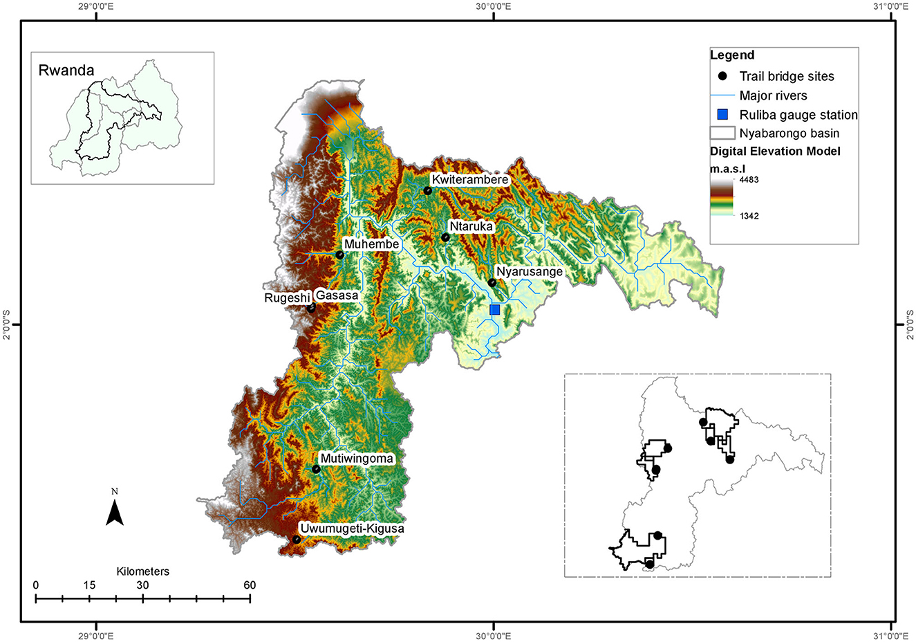
Figure 1. A map showing the Nyabarongo catchment and the trail bridge locations (black circles). The inset map at the bottom shows the approximate watershed of each of the bridge sites. The blue square symbol is the river gauge station at the Ruliba monitoring site along the Nyabarongo river which drains the entire catchment.

2.2. Data

2.2.1. In-situ observations

Three types of in-situ data were collected for bridge crossings analysis, streamflow modeling, and flood validation. The Browning Spec Ops Advantage (https://browningtrailcameras.com/) motion-activated cameras enabled with infrared capability were installed at the eight bridge sites to track and record pedestrian movement entering or exiting a bridge. The cameras were set to record 5-second videos and still pictures of objects passing through the bridges. The eight sites were part of the first wave of the randomized stepped-wedge impact evaluation design. The period of observation for the purpose of this study started in August 2021 and ended in July 2022, however, the cameras were intended to collect data until the end of the impact evaluation study in 2024. An earlier set of similar trail cameras were also used in the pilot study by Thomas et al. (2020), providing high-quality results when validated with data from manual counting devices.

Daily streamflow data was obtained from the Rwanda Water Resources Board (https://waterportal.rwb.rw). Considerable efforts have been made by RWB to improve the collection, archiving, and dissemination of streamflow data. The Ruliba station was instrumented with an automatic telemetry water level measuring station in 2018, improving the consistency and accuracy of streamflow measurements. The time series of the telemetry data extended from March 2018 to September 2022 (Figure 2). The telemetry stations measure the river stage which is then converted to streamflow or discharge using a rating curve derived from the observed stage and the associated discharge. Reported flood events data were provided by the Ministry in Charge of Emergency Management (MINEMA) covering the period between September 2013 and August 2022. These reports include the date of the flood event, and the reported impact including deaths, damages to infrastructure like bridges, schools, roads, etc., and losses experienced in farms among others.

FIGURE 2

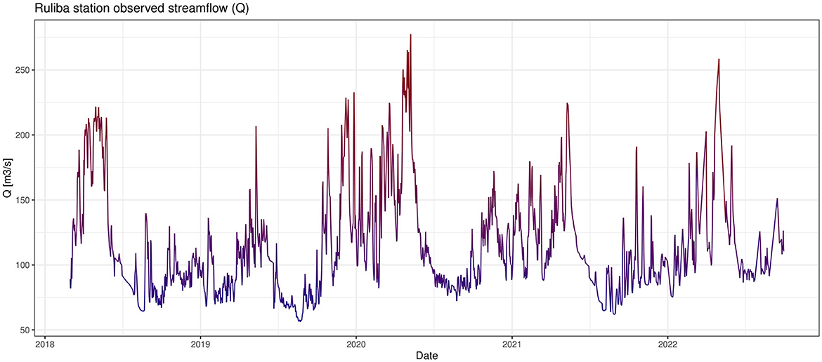
Figure 2. A hydrograph of the observed daily streamflow (Q) for the period 01/03/2018–30/09/2022.

2.2.2. Remote sensing observations

Gridded satellite rainfall data were retrieved from publicly available sources. For time series streamflow simulation and flood frequency analysis, we required gridded rainfall data covering the period 01/01/2001–31/12/2022. Three general types of satellite rainfall retrieval models are available for this type of research; data from gauge-corrected geostationary infrared sensors (Geo-IR) and passive-microwave sensors (PMW). The third model integrates PMW, Geo-IR, radar measurements, and gauge corrections. We used the daily Integrated Multi-Satellite Retrievals for the Global Precipitation Measurement (GPM) mission (IMERG-v06) late-run product available at a grid spacing of approximately 10 km (Huffman et al., 2020). The IMERG products are based on the third rainfall retrieval model. The choice of IMERG was informed by findings from an earlier study by our team highlighting the strengths of the integrated PMW-GeoIR-Radar-Gauge rainfall models in high-altitude areas (Macharia et al., 2022a). Specifically, that study revealed a better daily rainfall occurrence detection and intensity representation from the integrated models compared to Geo-IR models, characteristics that are non-trivial in hydrological modeling. The IMERG final product meets these characteristics but was only available up to 30/09/2021 at the time of data analysis for this study. We used the IMERG late-run data as a result which were downloaded from the SERVIR ClimateSERV data portal; https://climateserv.servirglobal.net/ (accessed January 2, 2023).

Daily gridded temperature data from the Climate Prediction Center (CPC) global temperature data provided by the US National Oceanic and Atmospheric Administration (NOAA) were downloaded from the International Research Institute for Climate and Society (IRI) Climate Data Library at http://iridl.ldeo.columbia.edu/SOURCES/ (accessed January 2, 2023). The data are the minimum and maximum temperature estimates available globally at 50 km spatial resolution. They contain gridded interpolated gauge measurements (Xie et al., 2010).

Soil moisture is an important variable in water balance models. It has been used to initialize model conditions, assimilated to improve model predictions, or generated as an output variable (Brocca et al., 2017). Daily volumetric soil moisture data were retrieved from the European Space Agency Climate Change Initiative (ESA-CCI) and the Copernicus Climate Change Service (C3S). The data have a spatial resolution of 25 km and are derived from radiometer (passive) and scatterometer (active) measurements (Dorigo et al., 2017; Gruber et al., 2019). We downloaded the combined product of the two measurements. The CCI product is available from 1978–2021 whereas the C3S product is available from 1978 to the present. The C3S product is derived from the CCI algorithm. We used the CCI product up to the end of 2021 and extended the time series with the C3S to cover the period from January–October 2022. This choice was made to minimize the area or the number of pixels with null values in the C3S product over the study area. By comparison, the CCI product is gap-filled, providing spatially complete estimates of soil moisture relative to the C3S product over the study area. The CCI and C3S data were retrieved from https://www.esa-soilmoisture-cci.org/node/145 and https://cds.climate.copernicus.eu/portfolio/dataset/satellite-soil-moisture, respectively (accessed January 2, 2023).

Monthly leaf area index (LAI) and normalized difference vegetation index (NDVI) from the Moderate Resolution Imaging Spectroradiometer (MODIS) aboard NASA's Terra and Aqua satellites were downloaded using the Google Earth Engine. Both vegetation indices are important variables for understanding the biological and physical processes associated with vegetated land surfaces and are key inputs in hydrological models (Wang et al., 2004). The LAI represents the green leaf area per unit ground area, an important property for understanding evapotranspiration processes in different vegetation types. The NDVI provides an estimate of vegetation photosynthetic activity and is known to account for the effects of soil and land cover changes on the rainfall-runoff response (Nourani et al., 2017). Both indices are available at various spatial resolutions but for the present study, we used the 500 m resolution product.

Soil data were downloaded from the Harmonized World Soil Database (Nachtergaele et al., 2008), containing fifteen soil properties for topsoil (0–30 cm) and subsoil (30–100 cm) at a grid resolution of 30 arc-sec (1 km). Landcover data was obtained from the Moderate-resolution Imaging Spectroradiometer (MODIS) global product at a 500-m grid resolution (Friedl et al., 2010). Elevation variables were obtained from the Shuttle Radar Topography Mission (SRTM) global Digital Elevation Model (DEM) at a grid resolution of 30 m. Wind speed data were obtained from the National Centers for Environmental Prediction (NCEP) reanalysis data at 2 m height and 250 km grid resolution. The input data is derived by combining eastward and northward wind vectors, represented by the variables “U” and “V” respectively.

2.3. Methods

Our methods included extreme rainfall analysis, streamflow modeling using a process-based and three machine learning models, flood frequency analysis, and correlation analysis to determine the associations between weather events and bridge use trends. These methods are summarized in the flowchart shown in Figure 3.

FIGURE 3

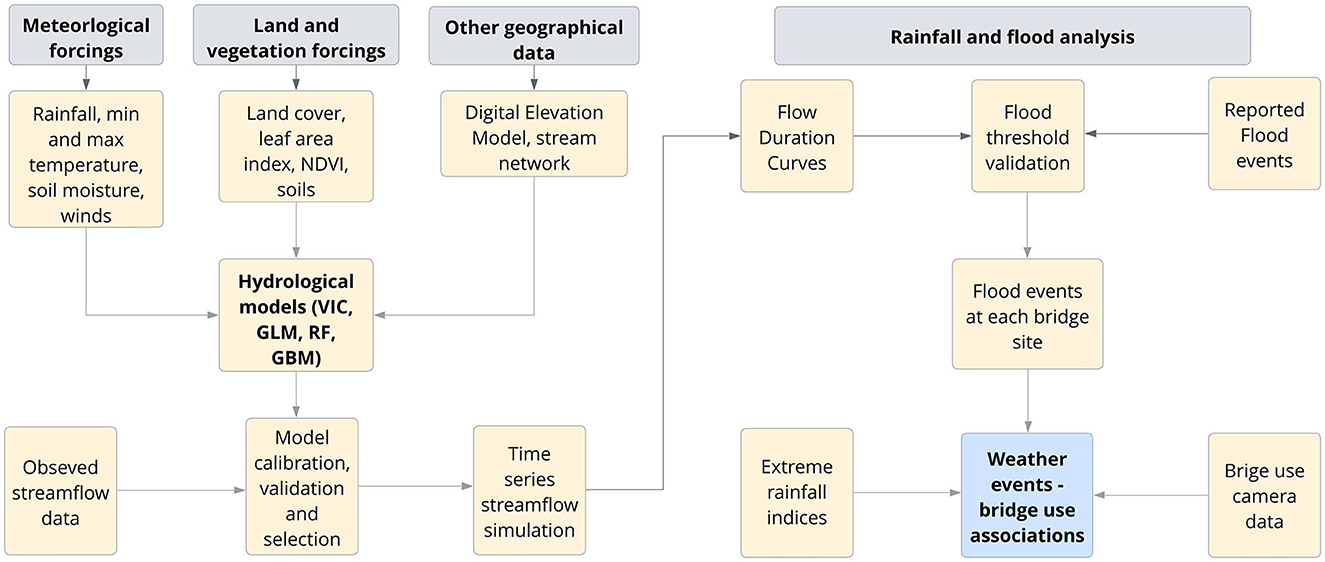
Figure 3. The general flowchart that we followed to carry out rainfall, streamflow, and bridge-use analysis. The acronyms VIC, GLM, RF, and GBM represent the Variable Infiltration Capacity model, Generalized Linear Model, Random Forest model, and Gradient Boosting Machine model, respectively.

2.3.1. Extreme rainfall indices

We constructed two extreme weather variables—number of very heavy precipitation days (R20mm) and Maximum daily rainfall amount (RX1day)—using the standardized approach recommended by the Expert Team on Climate Change Detection Indices (ETCCDI) (Donat et al., 2013). These indices were established by the World Meteorological Organization (WMO) and the World Climate Research Program (WCRP) to promote research on extreme climate events globally, eventually resulting in many studies of extreme events (e.g., Alexander et al., 2006; Ojara et al., 2021), including those focused on demographic behavior (e.g., Carrico et al., 2020). We also included rainfall anomalies to track changes in total annual rainfall over the past 20 years in the Nyabarongo catchment. This analysis was done using the Climate Data Operators (CDO) tool which is a collection of command line operators for analyzing and manipulating gridded climate data (Kaspar et al., 2010). Most ETCCDI studies use gauge station data where sufficient records are available, however, CDO provides the tools to carry out similar analyses using gridded time series satellite or climate model data. This is especially important for regions that have poor station data availability which is the case in the study area.

2.3.2. Streamflow modeling

Streamflow modeling is commonly done using approaches that rely on lumped, semi-, or fully distributed models. More recent approaches combine different types of models which are revolutionalizing hydrologic modeling (Xu and Liang, 2021), like in the case of hybrid process-based and machine learning models (Konapala et al., 2020; Yang et al., 2020; Huang et al., 2022). The machine learning (ML) models can be broadly classified as lumped models because they use input variables that are spatially aggregated at a basin or catchment scale. Distributed models estimate fluxes at a grid cell and then these fluxes, usually representing baseflow and runoff, are routed to a river channel connected to a pour point or basin outlet.

We followed a number of steps to estimate streamflow at the bridge sites. We set up our experiment in the Nyabarongo catchment where the bridges are located, and where we had observed daily streamflow data considered adequate for model training and validation. We then trained, validated, and compared the performance of the process-based semi-distributed Variable Infiltration Capacity (VIC) model (Liang et al., 1994) and three machine learning models: a Gradient Boosting Machine model (GBM) (Friedman, 2001), a Random Forest Model (RFM) (Breiman, 2001), and a Generalized Linear Model (GLM) (McCulloch, 2000). The VIC model solves water and energy fluxes over a gridded domain and a scheme that models how vegetation and soils control the fluxes. It has been used widely for flood and drought monitoring in small and large basins in sub-Saharan Africa, either as a standalone model (Sheffield et al., 2014; Shukla et al., 2014) or coupled with other models (Andreadis et al., 2017).

The VIC model was warmed up for a period of 2 years (01/01/2016–28/02/2018) to stabilize or reach an “optimal” state which is deemed important Kim et al. (2018). The observed streamflow was split into a calibration or training set (01/03/2018–28/02/2022) and a validation or testing set (01/03/2022–30/09/2022). There are contrasting arguments in the literature on the best approach for data splitting. Traditional approaches tend to take a proportional splitting whereas some more recent research advocates for the use of all available data in model calibration (Shen et al., 2022). Both approaches are influenced by the length of observed data and some discretion is required to determine the relevant approach to suit the modeling objectives. Our splitting approach above was intended to have as much data as possible during model calibration to capture recent very heavy rainfall events that resulted in extreme flooding between 2018 and 2022.

Gridded forcing data are required by the VIC model to solve the energy balance, generating baseflow and runoff amongst several other water, and land-atmosphere fluxes. The minimum inputs are rainfall, minimum and maximum temperature, wind speed, soil, land cover, LAI, and a digital elevation model (DEM) from which river network, slope, elevation, and flow direction layers are generated. The model further uses vegetation parameters and soil parameters generated from a combination of the vegetation and soil variables. The model was run at 2.5 km spatial resolution to simulate and calibrate streamflow output over 5000 iterations using the Shuffled Complex Evolution- University of Arizona (SCE-UA) algorithm (Duan et al., 1993, 1994). The VIC calibration was aimed at optimizing soil parameters which have been found to have the most significant impact on baseflow and runoff. The Lohmann routing algorithm (Lohmann et al., 1996, 1998) was coupled with the VIC model to route runoff and baseflow to get streamflow at the catchment outlet (Ruliba station).

The next step was to set up the ML models. All the VIC inputs except wind speed were used as input variables in the ML models in addition to soil moisture, NDVI, and LAI. The NDVI was used as a proxy for land cover and soils whereas the LAI was used to account for variability in evapotranspiration in the catchment. We also included lagged variables (1–3 days) of the soil moisture, rainfall, and temperature in the ML models to account for concentration times and the lagged response of streamflow to the climate variables (Shortridge et al., 2016; Xu and Liang, 2021). Unlike the VIC model, the ML models use spatially aggregated variables (Shortridge et al., 2016). The input variables were aggregated over the Nyabarongo catchment boundary using the mean statistic and maintaining the original spatial resolution of the input data before aggregation.

The ML models were implemented using the H2O package in R statistical tool (Team, 2013). The training and testing set were generated using random sampling i.e., we did not use the date split approach as for the VIC model, so a date in the observed time series streamflow was randomly allocated into either the training or testing set. Ten-fold cross-validation was used to develop and estimate the performance of the ML models using 75% of the observed streamflow data as the training sample. K-fold cross-validation is an important step in model development as it improves generalization by minimizing model error (Fushiki, 2011). The cross-validated models were then used to predict and validate the performance of the models with the remaining 25% of the data. Prior to model development, parameter optimization was done using the training set to select the best model parameters resulting in the lowest MAE and RMSE. This was only done for the RFM and GBM models, with the goal of optimizing the m_try, learning rate, and n-trees parameters. A standard model specification was adopted as given by Equation 1.

$\begin{array}{l}{Q}_{b,t}=f(P_{b,t},P_{b,t-1},P_{b,t-2},P_{b,t-3},T{n}_{b,t},T{n}_{b,t-1},T{n}_{b,t-2},\\ T{n}_{b,t-3},T{x}_{b,t},T{x}_{b,t-1},{\mathrm{Tx}}_{b,t-2},T{x}_{b,t-3},S{M}_{b,t},S{M}_{b,t-1},\\ S{M}_{b,t-2},S{M}_{b,t-3},LA{I}_{b,t},NDV{I}_{b,t})+{\epsilon }_{b,t},& (1)\end{array}$

where Q_{b, t} is the daily streamflow in river b at time period t; P_{b, t}, Tn_{b, t}, Tx_{b, t}, SM_{b, t} are the daily precipitation, minimum and maximum temperature, and soil moisture in river basin b at time period t; LAI_{b, t} and NDVI_{b, t} are the monthly average LAI and NDVI in basin b at time t; and ε_{b, t} is the model error. Lagged measurements represented by subscripts t−1, t−2, and t−3 were included to account roughly for concentration and storage times longer than 1 day that could impact streamflow in the river.

Whereas the main goal of streamflow modeling was to develop a model at the catchment scale, we explored methods to make a “best guess” of time series streamflow at the bridge sites; a major challenge due to the lack of observed river flows at the sites. Predicting streamflow in ungauged basins remains an area of great attention in hydrology, and many attempts have been made suggesting various approaches (Mohamoud, 2008; Atieh et al., 2017; Tegegne and Kim, 2018; Yilmaz and Onoz, 2020). Recognizing these challenges, we considered two general approaches. The first approach was to couple the watershed area ratio method Gianfagna et al. (2015), Ergen and Kentel (2016), Yilmaz and Onoz (2020) with the ML models, and the second approach was to couple the VIC model with the Lohmann flow routing scheme (Lohmann et al., 1996). Both approaches have been applied in hydrology where discharge observations are unavailable, inadequate, or of poor quality. These approaches share a similarity in that the discharge of a larger basin is a function of discharge at the smaller nested basins upstream of the larger basin outlet, and the flows are proportional to their watershed area. The watershed area ratio is calculated using 2;

$\begin{array}{ll}\begin{array}{ccc}WR& =\frac{Q_b}{A_b}& =\frac{Q_n}{A_n},\end{array}& (2)\end{array}$

where the ratio WR of discharge Q and the area A of basin b is equal to the ratio for nested basin n if both basins share a river network and have similarities in physiographic characteristics.

We used the Nash-Sutcliffe Efficiency (NSE) and the Kling-Gupta Efficiency (KGE) scores (Nash and Sutcliffe, 1970; Gupta et al., 2009) to evaluate the skill of the models in reproducing the observed flow hydrograph. We also included the Correlation Coefficient (r), Mean Absolute Error (MAE), Root Mean Squared Error (RMSE), and Percent Bias (PBIAS) as additional loss functions. The optimal values for these metrics are 1 for NSE and KGE, and 0 for MAE, RMSE, and PBIAS. These loss functions are used widely in hydrology to evaluate model performance (Moriasi et al., 2007).

2.3.3. Flood frequency analysis

Flood frequency analysis is useful for characterizing the streamflow regime of a catchment. This type of analysis is typical for applications in water resources planning such as irrigation, dam, and bridge constructions among others. One of the components of flood frequency analysis is the flood duration curve (FDC) which has relevance in calibrating hydrologic models (e.g., Westerberg et al., 2011) and validating hydrological extremes (Onyutha, 2012). The FDC shows the relationship between the frequency and duration of flood events for a specific location. By comparing both sets of data, the validity of the flood event can be determined. For example, if the observed flood event falls within the range of the predicted flood event data, as represented by the FDC, then the flood event can be considered valid. However, if the observed flood event falls outside of the expected range, then further investigation may be needed to determine the validity of the flood event. We adopted the FDC approach to identify flow thresholds upon which floods occur in the basin using the predicted streamflow time series from the methods described in Section 2.3.2 and the flood event data. Because of the similarities in physiographic characteristics across the catchment, we interpolated the flow thresholds to individual bridge sites and classified the streamflow values as either flood or non-flood events.

2.3.4. Bridge use

Pedestrian volumes were obtained by analyzing daily bridge crossings from the motion-activated cameras using a computer vision algorithm. This algorithm uses the open-source framework called Darknet that implements a pre-trained YOLO (You Only Look Once) (Redmon et al., 2016) deep neural network that has been trained to detect various objects, including people. This algorithm was trained and validated previously with traffic data from four bridges in Rwanda (Thomas et al., 2020). Results indicated a strong agreement between manual counting and computer-vision counting (R² range from 0.82–0.99, percent bias = 2.63%). Bridge crossings were aggregated at daily and monthly time scales for subsequent analysis. We only included days that had complete records i.e., 24 h of continuous tracking starting at 12:00 midnight.

3. Results and discussion

3.1. Extreme rainfall trends

Heavy rainfall has occurred in recent years leading to anomalously wet conditions that have had adverse consequences on lives, livelihoods, and transportation infrastructure. Figure 4 shows recent anomalous rainfall events across the country. There were widespread floods in the 2022 MAM season which caused losses and damages across the country. The season was one of the wettest in recent history, following similar events in 2018 and 2020 (Wainwright et al., 2020). The Nyabarongo catchment received an average of 116% [range from 92–146] of the normal annual rainfall whereas 2018 and 2020 events recorded 114% [range from 91–141%] and 104% [range from 84–133%] of the normal rainfall, respectively.

FIGURE 4

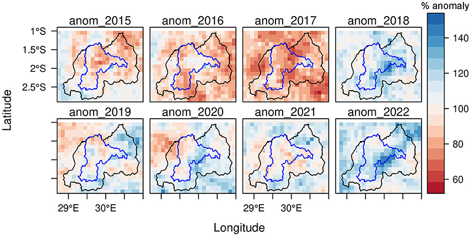
Figure 4. Annual rainfall anomalies across Rwanda expressed as a percentage of long-term mean annual rainfall. The blue polygon is the Nyabarongo catchment.

Focusing on extreme rainfall indices that cause flooding, our analysis revealed that the MAM season in 2018, 2020, and 2022, and the SOND season in 2019 had more very heavy rainfall days (R20mm) than the average of the season across many locations in the catchment (Figure 5). The maximum 1-day (Rx1day) rainfall amount in these seasons was not the highest in the last 20 years, however, the combination of high rainfall and more rainy days than normal resulted in the observed floods. This would seem to be the case for these seasons because flooding can occur when there is excessive rainfall over a short period of time, or when there is prolonged rain over several days. The streamflow hydrograph in Figure 2 is further evidence that the extreme rainfall events resulted in flood-generating flows. It also shows that the streamflow regime in this catchment is significantly influenced by rainfall.

FIGURE 5

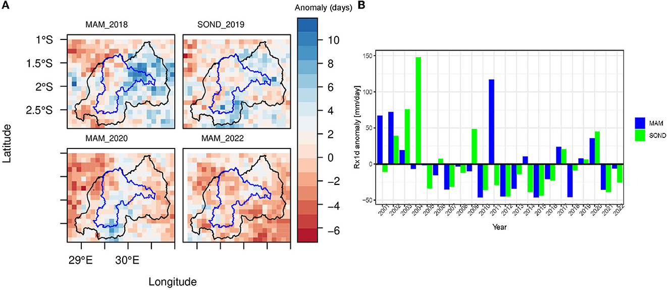
Figure 5. Extreme rainfall indices for the MAM and SOND rainy seasons for selected years. Maps (A) show the number of very heavy rainfall (R20mm) days above or below the long-term mean, whereas graph (B) shows the maximum 1-day rainfall (Rx1day) anomalies relative to the long-term mean maximum daily rainfall between 2001–2022.

Deaths and losses from these extreme events were reported across Western, Northern, and Southern Provinces. Data from the Ministry in charge of Emergency Management (MINEMA) showed that 13 people were killed and 25 bridges were damaged by the floods in 2018. Approximately 1,000 hectares of cropland were also destroyed in the three provinces. The impact on cropland doubled in the 2019 and 2020 floods while the number of deaths more than tripled relative to 2018. The 2022 flood events led to 39 deaths, and 24 bridges were also damaged (Figure 6). These flood events were preceded by droughts in 2015, 2016, and 2017, with the latter recording 83% of the annual normal rainfall. For the inhabitants of these provinces, recurrent floods and droughts compromise adaptation to climate variability.

FIGURE 6

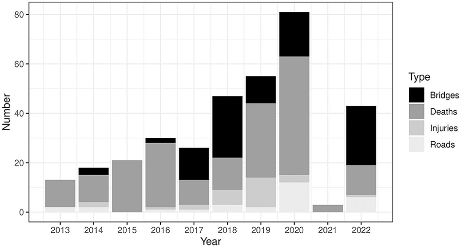
Figure 6. Flood impacts reported by the Rwanda Ministry in charge of Emergency Management (MINEMA) between 24/09/2013 and 17/08/2022 in Western, Northern, and Southern Provinces.

The main livelihood activity for communities in the three provinces is subsistence farming which is almost entirely reliant on rainfall. The terrain is hilly, and most farming is either on steep slopes (slope greater than 30%) or flood plains. Farming on this kind of terrain coupled with heavy rainfall exposes crops and the topsoil to erosion which can lead to loss of agricultural productivity. A recent study by Karamage et al. (2016) found that cropland was responsible for 95.8% of the total annual soil loss in the Nyabarongo catchment, with a mean erosion rate of 618 t/ha/yr. Soil erosion in Rwanda has also been associated with the siltation of streams and rivers downstream causing the reduction of river channel depth, and in turn, reducing the water holding capacity of the river channels (RWB and IUCN, 2022). Other compounding impacts of flooding in this catchment include contamination of drinking water through the transport of contaminants from point and non-point sources (Umwali et al., 2021). Market price hikes resulting from the disruption of supply chains due to damaged roads and reduced agricultural productivity (Kotz et al., 2022) can make it difficult for poor people exposed to flood and drought extremes to afford and sustain their needs.

3.2. Model evaluation

Results obtained from model validation are shown in Table 1. The Gradient Boosting Machine model had the best scores for all metrics, followed by the Random Forest Model and the Generalized Linear Model. These models outperformed the VIC simulations in all the metrics, however, it is important to note that the VIC errors are based on a validation set that did not present an exact corollary to the cross-validation set in the ML models. Nevertheless, the significantly large errors associated with the VIC model demonstrate the difficulty associated with the use of this model in the study area, particularly when relying on remote sensing datasets that may be unreliable at the resolution and accuracy required for process-based modeling in a catchment dominated by hilly terrain. Process-based models developed in the past over this catchment for daily peak flows and volumes have reported model errors comparable to our results. For example, an NSE value of 0.8 reported by Mind'je et al. (2019) compares well with NSE values ranging from 0.73–0.76 for the RFM and GBM models developed here. This is an impressive performance given that our focus was on both low and high flows which differs from the authors' focus on specific high-flow events. Predicting low flows remains a challenging area (Cenobio-Cruz et al., 2023), especially in mountainous regions like the Nyabarongo catchment where groundwater discharge dominates dry season streamflows (Somers and McKenzie, 2020).

TABLE 1

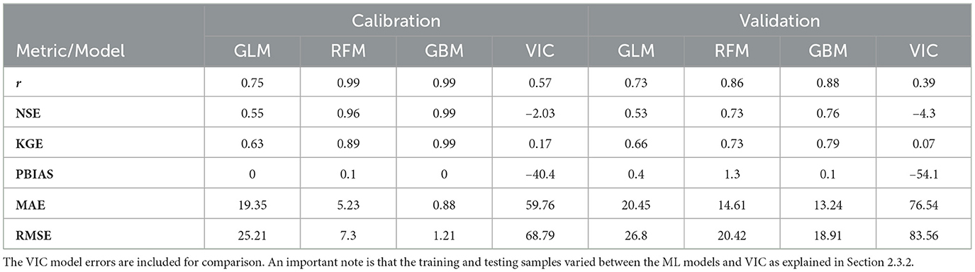
Table 1. Calibration and validation errors are shown for each model.

Soil moisture and vegetation variables had a higher importance across all the ML models compared to the rainfall and temperature variables as shown in Figure 7. This is an important finding for a number of reasons. Soil moisture is an important factor that affects streamflow prediction because it is a key component of the hydrologic cycle. Incorporating soil moisture data into a hydrologic model allows the model to take into account the current state of the soil and how much water is available for runoff. Prediction uncertainties may arise due to factors like errors in forcing data, the model's internal structure, and initial conditions. By taking soil moisture into account, the model can make more accurate predictions about how much runoff to expect given a certain amount of precipitation (Ding et al., 2022). Incorporating soil moisture data into hydrologic models can also help to mitigate the impact of errors in precipitation data on streamflow predictions (Kumar et al., 2021), and can minimize the uncertainties through better model initialization (Visweshwaran et al., 2022).

FIGURE 7

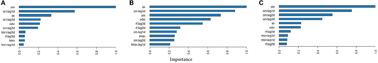
Figure 7. Variable importance for GBM (A), GLM (B), and RFM (C) models. The Y-axis represents the top ten variables ordered by the level of importance for that particular model. The acronyms are soil moisture (“sm”), leaf area index (lai), normalized difference vegetation index (“ndvi”), rainfall (“rf”), minimum temperature (“tmin”), and maximum temperature (“tmax”). Lag 1d, 2d, and 3d represent the lagged measurements of the associated variables.

It is however worth noting that soil moisture data itself can also be subject to measurement errors or uncertainties. Therefore, it is important to consider the quality and reliability of the soil moisture data when using it in hydrological models for streamflow prediction.

We achieved an improvement of the RMSE by 12% and the MAE by 16% when we included soil moisture in the GBM model which supports arguments in the literature that adding soil moisture in hydrological models improves streamflow and flood predictions (Brocca et al., 2010, 2017). The soil moisture data used in our study was evaluated by McNally et al. (2016) in East Africa for hydrological applications and found to be an acceptable alternative to remotely-sensed rainfall and NDVI commonly used for drought monitoring in moderately vegetated regions. We also found a high correlation between the soil moisture data and observed streamflow (r > 0.6), indicating the critical role that this variable plays in runoff-generating processes in the Nyabarongo catchment. This observation agrees with results from Kumar et al. (2021) who found the integration of the Advanced Scatterometer (ASCAT) soil moisture to have a remarkable improvement on streamflow predictions for poorly gauged catchments in India.

Another interesting finding is the combined dominant influence of soil moisture, LAI, and NDVI in the ML predictions. By excluding the three variables from the GBM model, the RMSE and MAE scores worsened by 102 and 108%, respectively whereas the KGE score worsened by 52% relative to the GBM model trained with the three variables present. We can conclude that the combined impact of soil moisture, land use, and land cover and their associated temporal variability on streamflow is substantial in the Nyabarongo catchment. It is also highly likely that the increase in errors when the three variables were excluded from the model was because the remaining variables; rainfall and temperature could not explain the variance in the observed streamflow because of the errors and the low correlations between the two, and observed streamflow. The Nyabarongo catchment has experienced substantial land use changes in the past two decades that could have significantly altered the land surface with an effect on surface runoff. Findings that the LAI and NDVI could be contributing substantially to the variance in the predicted streamflow are consistent with the conclusions made in past studies about the influence of the two variables on streamflow (Tesemma et al., 2015a,b; Ma et al., 2019; Mugo et al., 2020; Ding et al., 2022).

Figure 8 shows the simulated streamflow from the cross-validated models during the validation period. Note here that we do not include the VIC model hydrograph because of the aforementioned reason. We observed that the RFM (Figure 8B) and GBM (Figure 8C) models had larger errors for flow volumes greater than 150 m³/s whereas the errors were more pronounced for flow volumes less than 150 m³/s in the GLM model (Figure 8A). The likely explanation for these observations is that high flow volumes are more linearly influenced by rainfall and soil moisture conditions in the Nyabrongo catchment whereas low flows are influenced by groundwater discharge which nullifies the linear relationship between rainfall and streamflow. The GLM model is more sensitive to outliers than the GBM and RF models and as the results showed, it works well by predicting high flows in the catchment better than the two decision tree-based models. The GLM model underestimated the low flows as shown in the time series plot (Figure 8D) whereas all the models generally underestimated peak flow volumes. Nevertheless, these models reproduced the shape of the hydrograph well as shown by the high correlation coefficients and the KGE scores in Table 1.

FIGURE 8

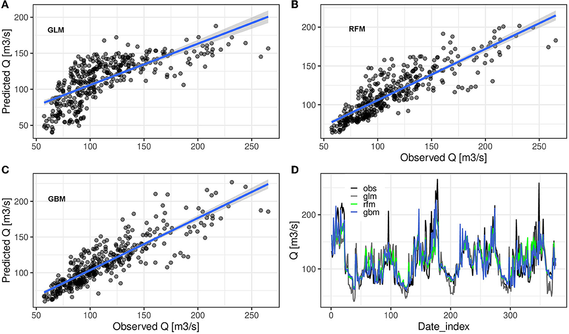
Figure 8. Scatterplots of observed and cross-validated streamflow (Q) predicted by the three machine learning models: GLM (A), RFM (B), and GBM (C). The time series plot (D) shows comparisons between the predictions and the observed streamflow (obs) for the validation set.

Further exploration of the VIC model errors was done by subjecting the GBM model to the same data samples for training and validation as those used by the VIC model. This was done in order to evaluate the performance of the ML models given the same time series as the VIC model. We found that the GBM model still outperformed the VIC model in all metrics. The KGE, MAE, and r scores for the GBM model were better than the VIC scores by a factor of 8, 2.7, and 1.6, respectively. The VIC RMSE score was 2.7 times worse than the GBM RMSE score. A promising finding from the VIC flow hydrograph was that it generally tracked low and high peaks quite well, despite the large volumetric errors that the model depicted. This observation is important for future improvements on the model and the shape of the hydrograph in Figure 9 seems to indicate a likely problem with the model's calibration of the soil depth parameters, probably due to errors in the soil rooting depth generated from the FAO Harmonized World Soils Database (HWSD). These parameters have an influence on the variable infiltration curve parameter which subsequently impacts runoff generation by the VIC model. Because the VIC model infiltration curve parameter calibration is sensitive to the accuracy of the soil layers, it is imperative to investigate and improve the accuracy of the HWSD data following recent findings by Ippolito et al. (2021) that found these data to have considerable discrepancies in the topsoil texture when compared with field data. Topsoil texture and composition are important factors in soil water holding capacity, and would directly impact the infiltration capacity and therefore runoff generation.

FIGURE 9

Figure 9. A plot showing the predicted time series for VIC and the GBM model compared with the observed streamflow for the validation period. The GBM model was configured to the same validation and testing sample as the VIC model for comparisons.

3.3. Flood frequency

Turning to the flood frequency analysis, we found that the annual maximum daily discharge in the Nyabarongo catchment has been on an upward trend in the last two decades (Figure 10B). This trend could be due to the following factors: (i) agricultural land expansion has been on the rise since the early 2000s with the highest land conversions occurring from forested, open, and wooded grasslands into croplands (Mugo et al., 2020; Bullock et al., 2021) and (ii), coupled with the frequency and severity of extreme rainfall, these conversions could have contributed to a reduction in the water holding or storage capacity of the soils which in turn increased surface runoff to rivers and other waterways. We noted a doubling of the annual runoff-to-rainfall ratio in the 20 years. We caution that this analysis was done using streamflow which includes baseflow; the ratio therefore may be more or less pronounced when the streamflow is partitioned into runoff and baseflow for a more realistic rainfall-runoff response relationship. We also note that the inference on landcover changes as a contributor to increasing peak annual runoff is supported by a recent study by Uwacu et al. (2021) indicating that soil erosion protection measures like terracing are not commonly practiced in the catchment which compromises surface runoff attenuation.

FIGURE 10

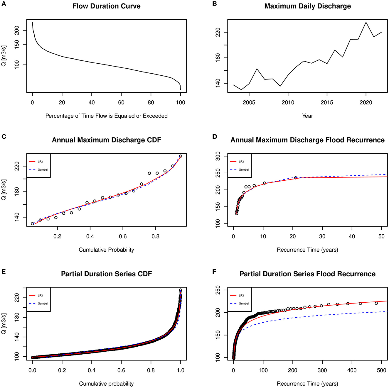
Figure 10. A series of graphs summarizing the flood frequency analysis. The graphs were generated using the time series streamflow predicted by the GBM model for 2003–2022. The partial duration series is generated by thresholding the entire time series of the predicted streamflow. The cutoff value was the 50% exceedance threshold of 98.33 m³/s; the value indicating flows that have a likelihood of 1 in 2 years of being exceeded. (A–F) Represent the Flow Duration Curve, Maximum Daily Discharge, Annual Maximum Discharge Cumulative Distribution Frequency, Annual Maximum Discharge Flood Recurrence, Partial Duration Series Cumulative Distribution Frequency, and Partial Duration Series Flood Recurrence, respectively.

The observed increasing trend in the annual runoff is also consistent with findings by Karamage et al. (2017) which found that Rwanda experienced a mean runoff depth increase of 2.33 mm/year between 1990 and 2016 with above-the-mean runoff depth increases experienced in districts in the Nyabarongo catchment including Ngororero and Gakenke. The authors attributed this increase to severe deforestation ranging between 62–85%, and cropland expansion ranging between 123–293%. Future extreme rainfall events will compound inappropriate land use practices that will further increase soil erosion and lower the stormwater retention capacity in the Nyabarongo catchment.

The Log-Pearson Type III (LP3) and Gumbel distributions indicate a similar pattern with the predicted discharge and flood occurrence return periods for the annual maximum discharge series (Figures 10C, D). Flood recurrence periods generated from the annual maximum daily discharge are appropriate for the design of extreme flood mitigation structures such as dikes, dams, and bridges. These are floods that occur very occasionally at the local level and the annual maximum discharge series would not be able to capture less extreme floods that cumulatively impact people more frequently. For this reason, we turn to Figures 10E, F which show the distribution and recurrence periods from a partial duration series generated by thresholding the entire time series of the predicted streamflow. The cutoff value was the 50% exceedance threshold (Figure 10A) which was 98.33 m³/s; the value indicating flows that have a likelihood of 1 in 2 years of being exceeded. The partial duration series is more appropriate for developing flood early warning systems due to its ability to capture low return period flows more accurately (Shortridge et al., 2016). This type of analysis would be relevant to a flood warning service that targets rural pedestrian movement and the development of anticipatory actions focused on mitigating lower magnitude but more frequent impacts.

For the design of flood early warning systems, and taking into account uncertainties related to the statistical model parameters, input data, and the rating curve model used to convert stage to streamflow, adopting the LP3 distribution function that generates higher flow values would be more appropriate for designing impact models associated with both low and high flow flood volumes.

From the flow duration curve and the flood recurrence plots in Figure 10 and Table 2, 90% of flood events reported between 2013 and 2022 were within the 50% exceedance threshold or 2-yr return period. This finding is consistent with observations made by Mind'je et al. (2019) and Mind'je et al. (2021) that high and moderate flows are the main factors associated with flooding incidences in the Nyabarongo catchment. More than a quarter of the reported floods (26%) were very extreme events in the 5% exceedance threshold (1 in 20 years return period) and most of them occurred between 14^th November and 12^th December 2019, and 12^th March and 16^th May 2020. According to a flood response report by One UN (CERF_Report) (accessed January 18, 2023), nearly 21,000 people were affected by these flood events, which also triggered landslides in affected places. There was widespread destruction of houses and livelihoods which resulted in humanitarian, health, and socio-economic vulnerabilities exacerbated by the COVID-19 pandemic. Most people who were rendered homeless were relocated to temporary shelters, mostly in schools.

TABLE 2

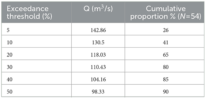
Table 2. This table shows the exceedance threshold, the associated streamflow value, and the percentage of flood events predicted by the GBM model.

As it has been observed since the early 2000s (MIDIMAR, 2015), the increasing impacts of floods and flood-related hazards will continue in the future making it extremely important to prioritize flood mitigation measures to save lives and livelihoods in these provinces. Projected rainfall from the Coupled Model Inter-comparison Project, Phase 5 (CIMP5) climate model ensembles indicate a likely increase in the intensity of heavy rainfall from 3 to 17%, and the frequency of these events is also expected to increase from 9 to 60% by the end of the century (World Bank Group, 2021). These increases are expected in most parts of the western, northern, and southern provinces.

3.4. Bridge use and weather events

The computer vision counted bridge crossings ranged from 1–1175 people per day with mean range crossings of 129–421 people per day (Table 3). The duration of observations ranged from 136–230 days. Comparisons between daily rainfall, streamflow, and daily bridge crossings did not indicate strong correlations but the correlations increased with temporal aggregation. Rugeshi, Nyarusange, and Mutiwingoma sites showed high but statistically insignificant (P > 0.05) correlations between total monthly crossings and total monthly rainfall (r= 0.58, 0.75, and 0.76, respectively) whereas Muhembe and Ntaruka had moderate correlations (r= 0.25 and 0.47, respectively). The rest of the bridges did not indicate any correlations. In terms of correlations between total monthly crossings and the total number of days in a month where streamflow exceeded the site flood threshold, Mutiwingoma, Muhembe, Rugeshi, and Uwumugeti had moderate to strong positive correlations (range from 0.36–0.84) whereas the rest of the bridges indicated moderate negative correlations (range from -0.33– -0.53).

TABLE 3

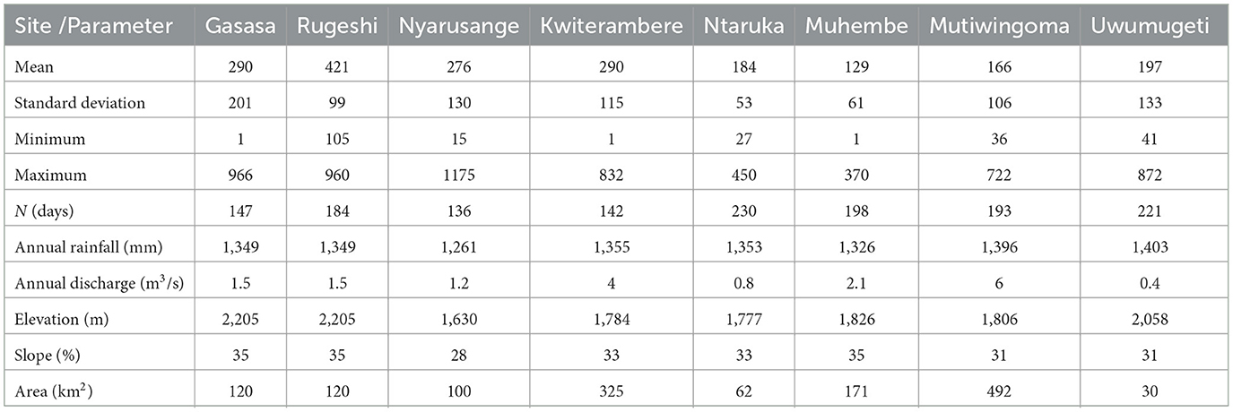
Table 3. Summary statistics of daily bridge crossings from motion-activated video clips at eight sites counted by a computer vision algorithm, and the physical characteristics of the sites.

These results indicate varying behavioral patterns across the bridge sites. The design intent of the trail bridges was to provide year-round transportation infrastructure for villages that are isolated during extreme rainfall events and periods of high river flows. Positive correlations between total rainfall and bridge crossings are indicative of the bridges providing the intended service. Negative correlations between the number of crossings and the total number of days with high river flows in some of the sites may be indicative of behavioral responses that point to people avoiding or minimizing travel during high rainfall months. It may also indicate that while the B2P bridges have the potential to contribute positively to the lives of the people in these sites, it may take some time before it influences the movement behavior of the people in these sites. The months with the highest bridge crossings across the sites were April, May, September, November, and December. The Famine Early Warning Systems Network (FEWS NET) crop calendar for Rwanda (https://fews.net/east-africa/rwanda; accessed January 22, 2023) identifies these months as the peak labor demand and migration periods for weeding (April, May, November, and December), and land preparation (September).

Baseline results from household surveys conducted in the impact evaluation study provide a strong case for the B2P bridge program in Rwanda. From the baseline study findings (Macharia et al., 2022b), 57% of the households across the three provinces had to cross rivers to reach hospitals and markets, and 25% to reach farmlands. Out of all the households, 42% worked outside their community, with the majority of these (63%) working in agriculture. By improving access for the dwellers of target villages, the trail bridges are expected to improve a number of outcomes including increasing agricultural productivity by eliminating flood risks, reducing travel time to markets and the cost of farm inputs as well as increasing wage earnings. This evidence is already available as demonstrated by the pilot study by Thomas et al. (2021) in the same locations and by similar outcomes in the Nicaragua trail bridge impact evaluation by Brooks and Donovan (2020). We plan to do a comprehensive analysis as more data from the cameras becomes available toward the end of the Rwanda impact evaluation study in 2024. This analysis will include linking the bridge use trends with household and site-level outcomes being measured via annual household surveys.

3.5. Limitations and future work

We relied on flow duration curves generated and validated at the catchment scale to interpolate flood thresholds to the individual bridge sites. For this reason, we caution readers that the lack of validation data at the bridge sites could be a source of errors. We also note that the model training and validation data covered a relatively wet period. While we believe that the dry period in part of 2019 and 2021 provided a counter-balance, it is important to continue to retrain and re-evaluate the models as more observed streamflow data become available. These limitations notwithstanding, the findings presented in this paper that associations between bridge use and weather events do exist in rural Rwanda present insights that can drive future research in this area. Findings that the machine learning models produce good skill in reproducing observed streamflow hydrograph reinforces published literature showing that empirical models have resulted in improved streamflow modeling, especially in places where process-based models do not perform well partly due to data constraints. However, we also find valid reasons for continuing VIC development by improving the quality of the meteorological forcing data, taking advantage of an increasing amount of remote sensing data that can be used to complement and bias correct the VIC inputs. We propose to adopt methods cited in the literature to make these improvements including but not limited to assimilating soil moisture data in the VIC model and using soil moisture data to correct rainfall data, among others.

Finally, we propose further work to improve VIC predictions by coupling the empirical models and VIC. Empirical studies have shown that the two types of models can be adapted to complement each other. One way is to use the ML models to predict residuals from the process-based, then use the predicted residuals to bias-correct the process-based predictions. That way, process understanding from the process-based is preserved while taking advantage of the strengths of the ML models in pattern learning to improve the predictions. Another approach is to partition streamflow into baseflow and runoff. Calibrating the VIC model for runoff could improve the simulations. There is sufficient evidence in the literature showing that partitioning the streamflow hydrograph and calibrating process-based models for runoff can improve predictive accuracy in regions where baseflows are a dominant component of the flow hydrograph. This is the case for western Rwanda where a significant amount of water flowing into the rivers comes from groundwater aquifers. Baseflows are high in the Nyabarongo catchment throughout the year but the VIC model's prediction of this streamflow component was poor, resulting in low values in most of the training, and validation periods. In a newly funded project, we will work with local government agencies and communities in the study area to advance the methods and lessons learned here to improve the models. This improvement is envisioned to contribute to the establishment of a flood early warning service connected to the B2P bridge infrastructure as a long-term flood risk mitigation measure.

4. Conclusions

In this study, we developed and compared the performance of two hydrologic models—three machine learning models (Generalized Linear Model, Random Forest Model, and Gradient Boosting Model) and one process-based (Variable Infiltration Capacity Model)— using remote sensing and in-situ streamflow data. We also validated model predictions of floods using observed flood event data in the Nyabarongo catchment. We then compared rainfall, flood events, and temporal bridge use in eight sites to investigate associations between weather events and bridge use traffic collected by motion-activated cameras.

The recent 2018, 2019, 2020, and 2022 wet extremes experienced in the Nyabarongo were associated with higher flood impacts relative to other rainfall events between 2013–2022. We found the machine learning models to perform relatively well compared to the process-based resulting in lower daily mean errors and a good replication of the observed streamflow hydrograph. The ML models had a KGE score range of 0.66–0.79 whereas the VIC model had a KGE score of 0.07. The model with the best skill was the Gradient Boosting Machine followed by the Random Forest model. From the GBM-simulated 20-year streamflow time series, the maximum annual daily streamflow associated with flooding depicted a steeply increasing trend with the probable explanation being a combination of both extreme rainfall and land use change.

We found that soil moisture and temporally varying vegetation variables improved the prediction of streamflow by the ML models. The overall model improvement in the KGE score was 52% when these variables were included in the GBM model. We found support for an existing association between weather and bridge use trends, with the highest bridge use being experienced during peak labor demand and migration months, which also coincided with the highest rainfall months. This trend may be indicative of mobility that is motivated by job opportunities available outside the source village. It may also indicate that mobility via the trail bridges to other places like markets and schools is highest during months with high total rainfall. We did not find clear associations between flood events and daily bridge use, however, we believe that these associations may be evident in the future when more bridge use data is available.

Data availability statement

The datasets used in this study can be found in the links provided in this article. Flood data was obtained from the Ministry in charge of Emergency Management and is not redistributable. The streamflow data was obtained from the Rwanda Water Resources Board portal (https://waterportal.rwb.rw/). The camera data is available from the authors upon request.

Ethics statement

This study was approved by the Rwanda National Ethics Committee (128/RNEC/2021) and the University of Colorado Boulder Institutional Review Board (20–0087). Written informed consent from the participants' legal guardian/next of kin was not required to participate in this study in accordance with the national legislation and the institutional requirements.

Author contributions

DM, LMa, and ET contributed to the conception and design of the study. LMu and AN participated in data collection. FK contributed to setting up the VIC model and reviewed data inputs and model outputs. DM and ET performed the statistical analysis. DM wrote the first draft of the manuscript. All authors contributed to the manuscript editing and approved the submitted version.

Funding

This study was funded by the United States Agency for International Development - Development Innovation Ventures under the terms of award No. 7200AA20FA00021, the Autodesk Foundation, and the Wellspring Foundation.

Acknowledgments

We acknowledge the contributions of Amazi Yego field staff for collecting camera data used in our analysis; colleagues at the Regional Centre for Mapping of Resources for Development (RCMRD) who provided expert advice on the hydrologic modeling plan, and the Rwanda Meteorology Agency (Meteo Rwanda), Rwanda Water Resources Board (RWB), and Ministry in charge of Emergency Management (MINEMA) for providing in-situ hydrometeorological data and flood statistics for model development. We also acknowledge Synaptiq for analyzing the camera data.

Conflict of interest

AN is a staff of the non-profit organization, Bridges to Prosperity, and is in charge of overseeing the construction of bridges in Rwanda. LMu is employed by Amazi Yego Ltd.

The remaining authors declare that the research was conducted in the absence of any commercial or financial relationships that could be construed as a potential conflict of interest.

Publisher's note

All claims expressed in this article are solely those of the authors and do not necessarily represent those of their affiliated organizations, or those of the publisher, the editors and the reviewers. Any product that may be evaluated in this article, or claim that may be made by its manufacturer, is not guaranteed or endorsed by the publisher.

References

Alexander, L. V., Zhang, X., Peterson, T. C., Caesar, J., Gleason, B., Klein Tank, A. M., et al. (2006). Global observed changes in daily climate extremes of temperature and precipitation. J. Geophys. Res. Atmosphere. 111, 6290. doi: 10.1029/2005JD006290

PubMed Abstract | CrossRef Full Text | Google Scholar

Andreadis, K. M., Das, N., Stampoulis, D., Ines, A., Fisher, J. B., Granger, S., et al. (2017). The regional hydrologic extremes assessment system: A software framework for hydrologic modeling and data assimilation. PLoS ONE 12, e176406. doi: 10.1371/journal.pone.0176506

PubMed Abstract | CrossRef Full Text | Google Scholar

Asefa, T., Kemblowski, M., McKee, M., and Khalil, A. (2006). Multi-time scale stream flow predictions: The support vector machines approach. J. Hydrol. 318, 7–16. doi: 10.1016/j.jhydrol.2005.06.001

CrossRef Full Text | Google Scholar

Atieh, M., Taylor, G. M. A, Sattar, A., and Gharabaghi, B. (2017). Prediction of flow duration curves for ungauged basins. J. Hydrol. 545, 383–394. doi: 10.1016/j.jhydrol.2016.12.048

CrossRef Full Text | Google Scholar

Best, K., Gilligan, J., Baroud, H., Carrico, A., Donato, K., and Mallick, B. (2022). Applying machine learning to social datasets: a study of migration in southwestern Bangladesh using random forests. Reg. Environ. Change 22, 52. doi: 10.1007/s10113-022-01915-1

CrossRef Full Text | Google Scholar

Bhusal, A., Parajuli, U., Regmi, S., and Kalra, A. (2022). Application of Machine Learning and Process-Based Models for Rainfall-Runoff Simulation in DuPage River Basin, Illinois. Hydrology 9, 117. doi: 10.3390/hydrology9070117

CrossRef Full Text | Google Scholar

Breiman, L. (2001). Random forests. Mach. Learn. 45, 5–32. doi: 10.1023/A:1010933404324

CrossRef Full Text | Google Scholar

Brocca, L., Ciabatta, L., Massari, C., Camici, S., and Tarpanelli, A. (2017). Soil moisture for hydrological applications: Open questions and new opportunities. Water 9, 140. doi: 10.3390/w9020140

CrossRef Full Text | Google Scholar

Brocca, L., Melone, F., Moramarco, T., Wagner, W., Naeimi, V., Bartalis, Z., et al. (2010). Improving runoff prediction through the assimilation of the ASCAT soil moisture product. Hydrol. Earth Syst. Sci. 14, 1881–1893. doi: 10.5194/hess-14-1881-2010

CrossRef Full Text | Google Scholar

Brooks, W., and Donovan, K. (2020). Eliminating uncertainty in market access: The impact of new bridges in rural nicaragua. Econometrica 88, 1965–1997. doi: 10.3982/ECTA15828

CrossRef Full Text | Google Scholar

Bullock, E. L., Healey, S. P., Yang, Z., Oduor, P., Gorelick, N., Omondi, S., et al. (2021). Three decades of land cover change in East Africa. Land 10, 1–15. doi: 10.3390/land10020150

CrossRef Full Text | Google Scholar

Call, M. A., Gray, C., Yunus, M., and Emch, M. (2017). Disruption, not displacement: Environmental variability and temporary migration in Bangladesh. Global Environ. Change 46, 157–165. doi: 10.1016/j.gloenvcha.2017.08.008

PubMed Abstract | CrossRef Full Text | Google Scholar

Carrico, A. R., Donato, K. M., Best, K. B., and Gilligan, J. (2020). Extreme weather and marriage among girls and women in Bangladesh. Global Environ. Change 65, 102160. doi: 10.1016/j.gloenvcha.2020.102160

CrossRef Full Text | Google Scholar

Cenobio-Cruz, O., Quintana-Seguí, P., Barella-Ortiz, A., Zabaleta, A., Garrote, L., Clavera-Gispert, R., et al. (2023). Improvement of low flows simulation in the SASER hydrological modeling chain. J. Hydrol. 18, 100147. doi: 10.1016/j.hydroa.2022.100147

CrossRef Full Text | Google Scholar

Dercon, S. (2002). Income Risk, Coping Strategies, and Safety Nets. Technical Report 2, The World Bank. doi: 10.1093/wbro/17.2.141

CrossRef Full Text | Google Scholar

Ding, Z., Lü, H., Ahmed, N., Zhu, Y., Gou, Q., Wang, X., et al. (2022). Soil moisture data assimilation in MISDc for improved hydrological simulation in upper Huai River Basin, China. Water 14, 3476. doi: 10.3390/w14213476

CrossRef Full Text | Google Scholar

Donat, M. G., Alexander, L. V., Yang, H., Durre, I., Vose, R., and Caesar, J. (2013). Global land-based datasets for monitoring climatic extremes. Bull. Am. Meteorol. Soc. 94, 997–1006. doi: 10.1175/BAMS-D-12-00109.1

CrossRef Full Text | Google Scholar

Dorigo, W., Wagner, W., Albergel, C., Albrecht, F., Balsamo, G., Brocca, L., et al. (2017). ESA CCI Soil Moisture for improved Earth system understanding: State-of-the art and future directions. Remote Sens. Environ. 203, 185–215. doi: 10.1016/j.rse.2017.07.001

CrossRef Full Text | Google Scholar

Duan, Q., Sorooshian, S., and Gupta, V. K. (1994). Optimal use of the SCE-UA global optimization method for calibrating watershed models. J. Hydrol. 158, 265–284. doi: 10.1016/0022-1694(94)90057-4

PubMed Abstract | CrossRef Full Text | Google Scholar

Duan, Q. Y., Gupta, V. K., and Sorooshian, S. (1993). Shuffled complex evolution approach for effective and efficient global minimization. J. Optimiz. Theory Applic. 76, 501–521. doi: 10.1007/BF00939380

CrossRef Full Text | Google Scholar

Ergen, K., and Kentel, E. (2016). An integrated map correlation method and multiple-source sites drainage-area ratio method for estimating streamflows at ungauged catchments: A case study of the Western Black Sea Region, Turkey. J. Environ. Manage. 166, 309–320. doi: 10.1016/j.jenvman.2015.10.036

PubMed Abstract | CrossRef Full Text | Google Scholar

Friedl, M. A., Sulla-Menashe, D., Tan, B., Schneider, A., Ramankutty, N., Sibley, A., et al. (2010). MODIS Collection 5 global land cover: Algorithm refinements and characterization of new datasets. Remote Sens. Environ. 114, 168–182. doi: 10.1016/j.rse.2009.08.016

CrossRef Full Text | Google Scholar

Friedman, J. (2001). Greedy function approximation: a gradient boosting machine. Ann. Statist. 29, 1189–1232. doi: 10.1214/aos/1013203451

CrossRef Full Text | Google Scholar

Fushiki, T. (2011). Estimation of prediction error by using K-fold cross-validation. Stat. Comput. 21, 137–146. doi: 10.1007/s11222-009-9153-8

CrossRef Full Text | Google Scholar

Gianfagna, C. C., Johnson, C. E., Chandler, D. G., and Hofmann, C. (2015). Watershed area ratio accurately predicts daily streamflow in nested catchments in the Catskills, New York. J. Hydrol. 4, 583–594. doi: 10.1016/j.ejrh.2015.09.002

CrossRef Full Text | Google Scholar

Grace, K., Hertrich, V., Singare, D., and Husak, G. (2018). Examining rural Sahelian out-migration in the context of climate change: An analysis of the linkages between rainfall and out-migration in two Malian villages from 1981 to 2009. World Develop. 109, 187–196. doi: 10.1016/j.worlddev.2018.04.009

CrossRef Full Text | Google Scholar

Gray, C., and Bilsborrow, R. (2013). Environmental influences on human migration in rural ecuador. Demography 50, 1217–1241. doi: 10.1007/s13524-012-0192-y

PubMed Abstract | CrossRef Full Text | Google Scholar

Gruber, A., Scanlon, T., Schalie, R. V. D., Wagner, W., and Dorigo, W. (2019). Evolution of the ESA CCI Soil Moisture climate data records and their underlying merging methodology. Earth Syst. Sci. Data 11, 717–739. doi: 10.5194/essd-11-717-2019

CrossRef Full Text | Google Scholar

Gupta, H. V., Kling, H., Yilmaz, K. K., and Martinez, G. F. (2009). Decomposition of the mean squared error and NSE performance criteria: Implications for improving hydrological modelling. J. Hydrol. 377, 80–91. doi: 10.1016/j.jhydrol.2009.08.003

CrossRef Full Text | Google Scholar

Huang, S., Xia, J., Wang, Y., Wang, W., Zeng, S., She, D., et al. (2022). Coupling machine learning into hydrodynamic models to improve river modeling with complex boundary conditions. Water Resour. Res. 58, 32183. doi: 10.1029/2022WR032183

CrossRef Full Text | Google Scholar

Huffman, G. J., Bolvin, D. T., Braithwaite, D., Hsu, K.-L., Joyce, R. J., Kidd, C., et al. (2020). “Integrated multi-satellite retrievals for the global precipitation measurement (GPM) mission (IMERG),” in Satellite Precipitation Measurement (Springer) 343–353. doi: 10.1007/978-3-030-24568-9_19

CrossRef Full Text | Google Scholar

Ippolito, T. A., Herrick, J. E., Dossa, E. L., Garba, M., Ouattara, M., Singh, U., et al. (2021). A comparison of approaches to regional land-use capability analysis for agricultural land-planning. Land 10, 458. doi: 10.3390/land10050458

CrossRef Full Text | Google Scholar

Karamage, F., Zhang, C., Fang, X., Liu, T., Ndayisaba, F., Nahayo, L., et al. (2017). Modeling rainfall-runoffresponse to land use and land cover change in Rwanda (1990-2016). Water 9, 147. doi: 10.3390/w9020147

CrossRef Full Text | Google Scholar

Karamage, F., Zhang, C., Kayiranga, A., Shao, H., Fang, X., Ndayisaba, F., et al. (2016). USLE-based assessment of soil erosion by water in the nyabarongo river catchment, Rwanda. Int. J. Environ. Res. Public Health 13, 835. doi: 10.3390/ijerph13080835

PubMed Abstract | CrossRef Full Text | Google Scholar

Kaspar, F., Schulzweida, U., and Müller, R. (2010). “Climate data operators' as a user-friendly processing tool for CM SAF's satellite-derived climate monitoring products,” in Conference: EUMETSAT Meteorological Satellite Conference 20–24.

Google Scholar

Kim, K. B., Kwon, H.-H., and Han, D. (2018). Exploration of warm-up period in conceptual hydrological modelling. J. Hydrol. 556, 194–210. doi: 10.1016/j.jhydrol.2017.11.015

CrossRef Full Text | Google Scholar

Konapala, G., Kao, S. C., Painter, S. L., and Lu, D. (2020). Machine learning assisted hybrid models can improve streamflow simulation in diverse catchments across the conterminous US. Environ. Res. Lett. 15, 104022. doi: 10.1088/1748-9326/aba927

CrossRef Full Text | Google Scholar

Kotz, M., Levermann, A., and Wenz, L. (2022). The effect of rainfall changes on economic production. Nature 601, 223–227. doi: 10.1038/s41586-021-04283-8

PubMed Abstract | CrossRef Full Text | Google Scholar

Kumar, A., Ramsankaran, R. A., Brocca, L., and Mu noz-Arriola, F. (2021). A simple machine learning approach to model real-time streamflow using satellite inputs: Demonstration in a data scarce catchment. J. Hydrol. 595, e126046. doi: 10.1016/j.jhydrol.2021.126046

CrossRef Full Text | Google Scholar

Liang, X., Lettenmaier, D. P., Wood, E. F., and Burges, S. J. (1994). A simple hydrologically based model of land surface water and energy fluxes for general circulation models. J. Geophys. Res. 99, 14415–14428. doi: 10.1029/94JD00483

CrossRef Full Text | Google Scholar

Lohmann, D., Raschke, E., and Lettenmaier, D. P. (1998). Regional scale hydrology: I. Formulation of the VIC-2L model coupled to a routing model. Hydrol. Sci. J. 43, 131–141. doi: 10.1080/02626669809492107

CrossRef Full Text | Google Scholar

Lohmann, D. A. G., Nolte-Holube, R., and Raschke, E. (1996). A large-scale horizontal routing model to be coupled to land surface parametrization schemes. Tellus A 48, 708–721. doi: 10.3402/tellusa.v48i5.12200

CrossRef Full Text | Google Scholar

Ma, T., Duan, Z., Li, R., and Song, X. (2019). Enhancing SWAT with remotely sensed LAI for improved modelling of ecohydrological process in subtropics. J. Hydrol. 570, 802–815. doi: 10.1016/j.jhydrol.2019.01.024

CrossRef Full Text | Google Scholar

Macharia, D., Fankhauser, K., Selker, J. S., Neff, J. C., and Thomas, E. A. (2022a). Validation and intercomparison of satellite-based rainfall products over Africa with TAHMO in-situ rainfall observations. J. Hydrometeorol. 23, 1131–1154. doi: 10.1175/JHM-D-21-0161.1

CrossRef Full Text | Google Scholar

Macharia, D., MacDonald, L., Mugabo, L., Donovan, K., Brooks, W., Gudissa, S., et al. (2022b). Mixed methods study design, pre-analysis plan, process evaluation and baseline results of trailbridges in rural Rwanda. Sci. Total Environ. 838, 156546. doi: 10.1016/j.scitotenv.2022.156546

PubMed Abstract | CrossRef Full Text | Google Scholar

McCulloch, C. E. (2000). Generalized linear models. J. Am. Statist. Assoc. 95, 1320–1324. doi: 10.1080/01621459.2000.10474340

CrossRef Full Text | Google Scholar

McLeman, R. (2013). Developments in modelling of climate change-related migration. Clim. Change 117, 599–611. doi: 10.1007/s10584-012-0578-2

PubMed Abstract | CrossRef Full Text | Google Scholar

McNally, A., Shukla, S., Arsenault, K. R., Wang, S., Peters-Lidard, C. D., and Verdin, J. P. (2016). Evaluating ESA CCI soil moisture in East Africa. Int. J. Appl. Earth Observ. Geoinform. 48, 96–109. doi: 10.1016/j.jag.2016.01.001

PubMed Abstract | CrossRef Full Text | Google Scholar

MIDIMAR (2015). The National Risk Atlas of Rwanda. Technical report, Ministry of Disaster Management and Refugee Affairs, Kigali, Rwanda.

Google Scholar

Mind'je, R., Li, L., Amanambu, A. C., Nahayo, L., Nsengiyumva, J. B., Gasirabo, A., et al. (2019). Flood susceptibility modeling and hazard perception in Rwanda. Int. J. Disaster Risk Reduct. 38, 101211. doi: 10.1016/j.ijdrr.2019.101211

CrossRef Full Text | Google Scholar

Mind'je, R., Li, L., Kayumba, P. M., Mindje, M., Ali, S., and Umugwaneza, A. (2021). Article integrated geospatial analysis and hydrological modeling for peak flow and volume simulation in rwanda. Water 13, 2926. doi: 10.3390/w13202926

CrossRef Full Text | Google Scholar

Mohamoud, Y. M. (2008). Prediction of daily flow duration curves and streamflow for ungauged catchments using regional flow duration curves. Hydrol. Sci. J. 53, 706–724. doi: 10.1623/hysj.53.4.706

PubMed Abstract | CrossRef Full Text | Google Scholar

Moriasi, D. N., Arnold, J. G., Liew, M. W. V., Bingner, R. L., Harmel, R. D., and Veith, T. L. (2007). Model evaluation guidelines for systematic quantification of accuracy in watershed simulations. Trans. ASABE 50, 885–900. doi: 10.13031/2013.23153

CrossRef Full Text | Google Scholar

Mugo, R., Waswa, R., Nyaga, J. W., Ndubi, A., Adams, E. C., and Flores-Anderson, A. I. (2020). Quantifying land use land cover changes in the lake victoria basin using satellite remote sensing: The trends and drivers between 1985 and 2014. Remote Sens. 12, 1–17. doi: 10.3390/rs12172829

CrossRef Full Text | Google Scholar

Nachtergaele, F. O., van Velthuizen, H., Verelst, L., Batjes, N. H., Dijkshoorn, J. A., van Engelen, V. W. P., et al. (2008). Harmonized World Soil Database (version 1.0). Rome: Food and Agric Organization of the UN (FAO); International Inst. for Applied Systems Analysis (IIASA); ISRIC - World Soil Information; Inst of Soil Science-Chinese Acad of Sciences (ISS-CAS); EC-Joint Research Centre (JRC).

Google Scholar

Nash, J. E., and Sutcliffe, J. V. (1970). River Flow Forecasting Through Conceptual Models Part I-A Discussion of Principles*. J. Hydrol. 10, 282–290. doi: 10.1016/0022-1694(70)90255-6

CrossRef Full Text | Google Scholar

Ndekezi, F.-X. (2012). Hydrological Modeling of Nyabarongo River Basin in Rwanda: Using Combination of Precipitation Input from Meteorological Models, Remote Sensing, and Ground Station Measurement. Technical report, LAP LAMBERT Academic Publishing.

Google Scholar

Nourani, V., Fard, A. F., Gupta, H. V., Goodrich, D. C., and Niazi, F. (2017). Hydrological model parameterization using NDVI values to account for the effects of land cover change on the rainfall-runoff response. Hydrol. Res. 48, 1455–1473. doi: 10.2166/nh.2017.249

CrossRef Full Text | Google Scholar

Ojara, M. A., Yunsheng, L., Babaousmail, H., and Wasswa, P. (2021). Trends and zonal variability of extreme rainfall events over East Africa during 1960–2017. Natural Hazards 109, 33–61. doi: 10.1007/s11069-021-04824-4

CrossRef Full Text | Google Scholar

Onyutha, C. (2012). Statistical modelling of FDC and return periods to characterise QDF and design threshold of hydrological extremes. J. Urban Environ. Eng. 6, 132–148. doi: 10.4090/juee.2012.v6n2.132148

CrossRef Full Text | Google Scholar

Pechlivanidis, I. G., Jackson, B. M., Mcintyre, N. R., and Wheater, H. S. (2011). Catchment scale hydrological modelling: a review of model types, calibration approaches and uncertainty analysis methods in the context of recent developments in technology and applications. Global NEST J. 13, 193–214. doi: 10.30955/gnj.000778

CrossRef Full Text | Google Scholar

Redmon, J., Divvala, S., Girshick, R., and Farhadi, A. (2016). “You only look once: Unified, real-time object detection,” in Proceedings of the IEEE Computer Society Conference on Computer Vision and Pattern Recognition. doi: 10.1109/CVPR.2016.91

CrossRef Full Text | Google Scholar

RWB and IUCN (2022). The State of Soil Erosion Control in Rwanda. Technical report, Rwanda Water Board, Kigali.

Google Scholar

Sheffield, J., Wood, E. F., Chaney, N., Guan, K., Sadri, S., Yuan, X., et al. (2014). A drought monitoring and forecasting system for sub-Sahara African water resources and food security. Bull. Am. Meteorol. Soc. 95, 861–882. doi: 10.1175/BAMS-D-12-00124.1

CrossRef Full Text | Google Scholar

Shen, H., Tolson, B. A., and Mai, J. (2022). Time to update the split-sample approach in hydrological model calibration. Water Resour. Res. 58, e2021WR031523. doi: 10.1029/2021WR031523

CrossRef Full Text | Google Scholar

Shirley, K., Noriega, A., Levin, D., and Barstow, C. (2021). Identifying water crossings in rural liberia and rwanda using remote and field-based methods. Sustainability 13, 527. doi: 10.3390/su13020527

CrossRef Full Text | Google Scholar

Shortridge, J. E., Guikema, S. D., and Zaitchik, B. F. (2016). Machine learning methods for empirical streamflow simulation: A comparison of model accuracy, interpretability, and uncertainty in seasonal watersheds. Hydrol. Earth Syst. Sci. 20, 2611–2628. doi: 10.5194/hess-20-2611-2016

CrossRef Full Text | Google Scholar

Shukla, S., McNally, A., Husak, G., and Funk, C. (2014). A seasonal agricultural drought forecast system for food-insecure regions of East Africa. Hydrol. Earth Syst. Sci. 18, 3907–3921. doi: 10.5194/hess-18-3907-2014

CrossRef Full Text | Google Scholar

Solomatine, D. P., and Wagener, T. (2011). “2.16 - Hydrological Modeling,” in Treatise on Water Science, eds. P., Wilderer (Oxford: Elsevier) 435–457. doi: 10.1016/B978-0-444-53199-5.00044-0

CrossRef Full Text | Google Scholar

Somers, L. D., and McKenzie, J. M. (2020). A review of groundwater in high mountain environments. Wiley Interdisc. Rev. 7, e1475. doi: 10.1002/wat2.1475

CrossRef Full Text | Google Scholar

Starkey, P. (2002). Improving rural mobility: options for developing motorized and nonmotorized transport in rural areas. Technical report, World Bank. doi: 10.1596/0-8213-5185-0

CrossRef Full Text | Google Scholar

Starkey, P. (2016). The benefits and challenges of increasing motorcycle use for rural access. Technical report, World Bank.

PubMed Abstract | Google Scholar

Team, R. C. (2013). R: A language and environment for statistical computing.

Google Scholar

Tegegne, G., and Kim, Y. O. (2018). Modelling ungauged catchments using the catchment runoff response similarity. J. Hydrol. 564, 452–466. doi: 10.1016/j.jhydrol.2018.07.042

CrossRef Full Text | Google Scholar

Tesemma, Z. K., Wei, Y., Peel, M. C., and Western, A. W. (2015a). Including the dynamic relationship between climatic variables and leaf area index in a hydrological model to improve streamflow prediction under a changing climate. Hydrol. Earth Syst. Sci. 19, 2821–2836. doi: 10.5194/hess-19-2821-2015

CrossRef Full Text | Google Scholar

Tesemma, Z. K., Wei, Y., Peel, M. C., and Western, A. W. (2015b). The effect of year-to-year variability of leaf area index on Variable Infiltration Capacity model performance and simulation of runoff. Adv. Water Resour. 83, 310–322. doi: 10.1016/j.advwatres.2015.07.002

CrossRef Full Text | Google Scholar

Thomas, E., Bradshaw, A., Mugabo, L., MacDonald, L., Brooks, W., Dickinson, K., et al. (2021). Engineering environmental resilience: A matched cohort study of the community benefits of trailbridges in rural Rwanda. Sci. Total Environ. 771, 145275. doi: 10.1016/j.scitotenv.2021.145275

PubMed Abstract | CrossRef Full Text | Google Scholar

Thomas, E., Gerster, S., Mugabo, L., Jean, H., and Oates, T. (2020). Computer vision supported pedestrian tracking: A demonstration on trail bridges in rural Rwanda. PLoS ONE 15, e0241379. doi: 10.1371/journal.pone.0241379

PubMed Abstract | CrossRef Full Text | Google Scholar

Umwali, E. D., Kurban, A., Isabwe, A., Mind'je, R., Azadi, H., Guo, Z., et al. (2021). Spatio-seasonal variation of water quality influenced by land use and land cover in Lake Muhazi. Sci. Rep. 11, 17376. doi: 10.1038/s41598-021-96633-9

PubMed Abstract | CrossRef Full Text | Google Scholar

Uwacu, R. A., Habanabakize, E., Adamowski, J., and Schwinghamer, T. D. (2021). Using radical terraces for erosion control and water quality improvement in Rwanda: A case study in Sebeya catchment. Environ. Develop. 39, 649. doi: 10.1016/j.envdev.2021.100649

CrossRef Full Text | Google Scholar

Visweshwaran, R., Ramsankaran, R. A., Eldho, T. I., and Lakshmivarahan, S. (2022). Sensitivity-based soil moisture assimilation for improved streamflow forecast using a novel forward sensitivity method (FSM) approach. Water Resour. Res. 58, 92. doi: 10.1029/2021WR031092

CrossRef Full Text | Google Scholar

Wainwright, C. M., Finney, D. L., Kilavi, M., Black, E., and Marsham, J. H. (2020). Extreme rainfall in East Africa, October 2019–January 2020 and context under future climate change. Weather 76, 26–31. doi: 10.1002/wea.3824

CrossRef Full Text | Google Scholar

Wang, Y., Woodcock, C. E., Buermann, W., Stenberg, P., Voipio, P., Smolander, H., et al. (2004). Evaluation of the MODIS LAI algorithm at a coniferous forest site in Finland. Remote Sens. Environ. 91, 114–127. doi: 10.1016/j.rse.2004.02.007

CrossRef Full Text | Google Scholar

Westerberg, I. K., Guerrero, J. L., Younger, P. M., Beven, K. J., Seibert, J., Halldin, S., et al. (2011). Calibration of hydrological models using flow-duration curves. Hydrol. Earth Syst. Sci. 15, 2205–2227. doi: 10.5194/hess-15-2205-2011

PubMed Abstract | CrossRef Full Text | Google Scholar

World Bank Group (2021). Rwanda Climate Risk Country Profile. Technical report, World Bank, Washington, DC.

Google Scholar

Xie, P., Chen, M., and Shi, W. (2010). “CPC unified gauge-based analysis of global daily precipitation,” in 24th Conference on Hydrology, Atlanta, GA, Amer. Meteor. Social 2.

Google Scholar

Xu, T., and Liang, F. (2021). Machine learning for hydrologic sciences: An introductory overview. Wiley Interdisc. Rev. 8, e1533. doi: 10.1002/wat2.1533

CrossRef Full Text | Google Scholar

Yang, S., Yang, D., Chen, J., Santisirisomboon, J., Lu, W., and Zhao, B. (2020). A physical process and machine learning combined hydrological model for daily streamflow simulations of large watersheds with limited observation data. J. Hydrol. 590, 125206. doi: 10.1016/j.jhydrol.2020.125206

CrossRef Full Text | Google Scholar

Yilmaz, M. U., and Onoz, B. (2020). A comparative study of statistical methods for daily streamflow estimation at ungauged basins in Turkey. Water 12, 459. doi: 10.3390/w12020459

CrossRef Full Text | Google Scholar