Finite-Time Stability of Hybrid Systems With Unstable Modes

1 Introduction

Stability of the equilibrium point or equilibrium set of switched and hybrid systems has been studied extensively in the literature. In Branicky (1998), the author introduces the concept of multiple Lyapunov functions to analyze stability of switched systems; since then, a lot of work has been done on the topic, see e.g., (Zhao and Hill, 2008); Zhao et al., 2012). In Zhao and Hill (2008), the authors relax the non-increasing condition on the Lyapunov functions used in (Branicky, 1998), by introducing the notion of generalized Lyapunov functions. They present necessary and sufficient conditions for Lyapunov and asymptotic stability (AS) of switched systems under arbitrary switching. Inspired by the results in (Branicky, 1998; Zhao and Hill, 2008), we study conditions for finite-time stability (FTS)¹ of a class of hybrid systems, using multiple generalized Lyapunov functions. In contrast to AS, which pertains to convergence as time tends to infinity, FTS is a concept that requires convergence of solutions in finite time. FTS is a well-studied concept, motivated in part from a practical viewpoint due to properties such as convergence in finite time, as well as robustness with respect to disturbances (Ryan, 1991). In the seminal work (Bhat and Bernstein, 2000), the authors introduce necessary and sufficient conditions in terms of Lyapunov functions for continuous, autonomous systems to exhibit FTS.

FTS of switched and hybrid systems has gained popularity in the last few years. The authors in Liu et al. (2017) consider the problem of designing a controller for a linear switched system under delay and external disturbance with finite-time convergence. The authors in Li and Sanfelice (2019) present conditions in terms of a common Lyapunov function for FTS of hybrid systems. They require the value of the Lyapunov function to be decreasing during the continuous flow and non-increasing at the discrete jumps. The authors in Ríos et al. (2015) design an FTS state observer for switched systems via a sliding-mode technique under the assumption that each individual subsystem is observable on a domain. More recently, the authors in Zhang (2018) study FTS of homogeneous switched systems by introducing the concept of hybrid homogeneous degree, and relating negative homogeneity with FTS. They consider switched systems with an assumption that each subsystem possess a homogeneous Lyapunov function, and that the switching-intervals are constant.

In this paper, we develop sufficient conditions for FTS of a class of hybrid systems in terms of multiple Lyapunov functions. To the best of authors’ knowledge, this is the first work considering FTS of hybrid systems using multiple Lyapunov functions. We first define the notion of FTS for hybrid systems in a way that does not restrict each mode of the hybrid system to be FTS in itself. More specifically, we relax the requirement in (Zhao and Hill, 2008; Li and Sanfelice, 2019) that each Lyapunov function is non-increasing at the discrete jumps, and strictly decreasing during the continuous flow; instead, we allow the Lyapunov functions to increase both during the continuous flow and at the discrete jumps, and require that these increments are bounded. In this respect, we allow the hybrid system to have unstable modes while still guaranteeing FTS. In addition, we present a novel proof on the stability of the origin using multiple Lyapunov functions under the aforementioned relaxed conditions. As compared to Zhang (2018), in the current paper we do not assume that the subsystems are homogeneous or in strict feedback form. The main result is that if the origin is stable under arbitrary switching, and if there exists an FTS mode that is active for a sufficient cumulative time, then the origin of the resulting hybrid system is FTS. As thus, the results in Bhat and Bernstein (2000) on FTS of continuous systems are a special case of the proposed results. The paper also extends and generalizes the results of the authors’ prior work in (Garg and Panagou, 2021) where FTS of a class of switched system is studied.

The motivation of studying FTS using multiple Lyapunov functions comes from applications where the switching law is not under the user’s control authority, or where keeping the FTS mode active for a long period leads to undesirable behavior. As an example, consider a spacecraft that tracks a desired trajectory, with the on-board communication and the controller module requiring a certain minimum energy threshold to function. The charge-level of the spacecraft battery can be modeled as a hybrid system, where being in the path of sunlight would be an FTS mode, leading to increase in the charging level, and tracking the desired trajectory an unstable mode since it depletes the charge. Now, keeping the FTS mode active for a long duration might lead to the spacecraft losing track of its desired trajectory, and thus, the switching signal between the two modes cannot be designed arbitrarily. At the same time, FTS is desired so that the spacecraft can activate its communication module for crucial communications with the ground station and/or the control module to compute inputs for the next part of the journey. Thus, for the applications where the FTS mode cannot be kept active for all times, or the switching signal is not under user’s control, it is essential to study FTS under switching laws that allow the FTS mode to become inactive, and unstable modes to become active.

2 Finite-Time Stability of Hybrid Systems

2.1 Preliminaries

We denote by ‖ ⋅ ‖ the Euclidean norm of vector (⋅), |⋅| the absolute value if (⋅) is scalar and the length if (⋅) is a time interval. The set of non-negative reals is denoted by ${\mathbb{R}}_{+}$, set of non-negative integers by ${\mathbb{Z}}_{+}$ and set of positive integers by $\mathbb{N}$. We denote by int(S) the interior of the set S. The right and left limits of the function $x:\mathbb{R}\to {\mathbb{R}}^n$ are given by x (t⁻) = lim_τ↗tx(τ) and x (t⁺) = lim_τ↘tx(τ) respectively.

Definition: A continuous function $\alpha :{\mathbb{R}}_{+}\to {\mathbb{R}}_{+}$ is called.

• Class-$\mathcal{K}$function: if it is increasing, i.e., for all x > y ≥ 0, α(x) > α(y);

• Class-${\mathcal{K}}_{\infty }$function: if it is a class-$\mathcal{K}$ function, and lim_r→∞α(r) = ∞.

Next, we review the notion of FTS. Consider the system:

$x(t)=f(x(t)),(1)$

where $x\in {\mathbb{R}}^n$, $f:\mathcal{D}\to {\mathbb{R}}^n$ is continuous on an open neighborhood $\mathcal{D}\subseteq {\mathbb{R}}^n$ of the origin and f (0) = 0. Assume that the solution of Eq. 1 exists and is unique. The origin is said to be an FTS equilibrium of Eq. 1 if it is Lyapunov stable and for all $x(0)\in \mathcal{N}\backslash \{0\}$, where $\mathcal{N}\subset \mathcal{D}$ is some open neighborhood of the origin, lim_t→T x(t) = 0, where T = T (x (0)) < ∞ [see (Bhat and Bernstein, 2000)]. The authors also presented Lyapunov conditions for FTS of the origin of Eq. 1:

Theorem 1: [Bhat and Bernstein (2000)].Suppose there exist a continuously differentiable, positive definite function$V:\mathcal{D}\to \mathbb{R}$forEq. 1, real numbersc > 0 andα ∈ (0, 1), and an open neighborhood$\mathcal{V}\subseteq \mathcal{D}\subset {\mathbb{R}}^n$of the origin such that

$V(x)\le -cV{(x)}^{\alpha },x\in \mathcal{V}\backslash \{0\}.(2)$

Then the origin is an FTS equilibrium.

We state the following Lemma before we proceed to the main results, which follows from (Zuo and Tie, 2016, Lemma 3.3).

Lemma 1:Leta_i ≥ b_i ≥ 0 for alli ∈{1, 2, … , K} for some$K\in \mathbb{N}$. Then, for any 0 < r < 1, we have

$\sum _{i=1}^K(a_i^r-b_i^r)\le \sum _{i=1}^K{(a_i-b_i)}^r.(3)$

2.2 Main Results

We consider the class of hybrid systems $\mathcal{H}=\{C,\mathcal{F},D,\mathcal{G}\}$ described as

$\begin{array}{cc}\hfill x(t)& =f_{{\sigma }_f(t,x)}(x(t)),x(t)\in C,\hfill \\ \hfill x(t^{+})& =g(x(t^{-})),x(t)\in D,\hfill \end{array}(4)$

where $x\in {\mathbb{R}}^n$ is the state vector with x (t₀) = x₀, $f_i\in \mathcal{F}\triangleq \{f_k:{\mathbb{R}}^n\to {\mathbb{R}}^n\}$ for k ∈ Σ_f ≜{1, 2, … , N_f} is the continuous flow (called thereafter, subsystem, or mode) allowed on the subset of the state space $C\subset {\mathbb{R}}^n$, and $\mathcal{G}=\{g\}$ where $g:{\mathbb{R}}^n\to {\mathbb{R}}^n$ defines the discrete behavior (called thereafter discrete-jump dynamics), which is allowed on the subset $D\subset {\mathbb{R}}^n$. Note that at the jump instant $t\in {\mathbb{R}}_{+}$, the state x(t) is characterized by multiple values, namely the value just before the jump at time t, which we denote as x (t⁻), and the value just after the jump at time t, which we denote as x (t⁺) (satisfying x (t⁺) = g (x (t⁻))). The switching signal ${\sigma }_f:{\mathbb{R}}_{+}\times {\mathbb{R}}^n\to {\mathrm{\Sigma }}_f$ is assumed to be continuous in x and piecewise continuous (from the right) in t. We omit the argument (t, x) from σ_f for the sake of brevity. Systems of the form Eq. 4 have been studied in (Branicky, 1998), while Zhao and Hill (2008) considers the form Eq. 4 without the discrete-jump dynamics.

Denote by $T_{i_k}=[t_{i_k},t_{i_k+1})\subset {\mathbb{R}}_{+}$, with $t_{i_k+1}\ge t_{i_k}\ge t_0$, the interval in which the flow f_i is active for the k−th time for i ∈Σ_f and $k\in \mathbb{N}$, and $t=t_m^d$ the time when discrete jump x (t⁺) = g (x (t⁻)) takes place for the m−th time, $m\in \mathbb{N}$. Define $J_i=\{t_m^d|t_m^d\in T_{i_k},m\in \mathbb{N}\}$ as the set of all time instances when a discrete jump takes place when the continuous flow f_i is active, and $\mathcal{J}=\bigcup _{i\in {\mathrm{\Sigma }}_f}{J}_i$ as the set of all times when the state of Eq.4 undergoes a discrete jump. Without loss of generality, we assume that the switching signal σ_f is minimal, i.e., for any i ∈ Σ_f, $t_{i_{k+1}}\ne t_{i_k+1}$ for all $k\in \mathbb{N}$, and that there are no two discrete jumps at the same time instant. We also make the following assumption.

Assumption 1.The functionsf_iare continuous for alli ∈Σ_fand the origin is the unique equilibrium point ofEq. 4.

The case when there exists a closed set $D\ne \{0\}$ such that g(x) = 0 for all $x\in D\subset D$ can be treated by studying stability of closed sets; see (Li and Sanfelice, 2019). The solution of the hybrid system Eq. 4 can be defined as follows: a function $x:{\mathbb{R}}_{+}\to {\mathbb{R}}^n$ is a solution of Eq. 4 if.

• it is absolutely continuous between any two jump instants and satisfies $x(t)=f_k(t,x)$ for almost all $t\in {\mathbb{R}}_{+}\backslash \mathcal{J}$ such that x(t) ∈ C, where k = σ(t, x);

• it satisfies x (t⁺) = g (x(t)), for all $t\in \mathcal{J}$ such that x(t) ∈ D.

Interested reader is referred to (Goebel et al., 2012, Chapter 2) for a detailed presentation on solution notion of hybrid systems. We assume that the solution of Eq. 4 exists for all t ≥ 0, and is non-Zeno². Similar assumptions have been used in literature (e.g., Zhao and Hill, 2008; Li and Sanfelice, 2019; Sanfelice et al., 2007) in order to analyze stability properties of the origin of hybrid systems.

Next, we define the notion of FTS for hybrid systems. Note that a mode F ∈Σ_f is called an FTS subsystem or FTS mode if the origin of $\dot{y}=f_F(y)$ is FTS. The notion of stability for switched systems under arbitrary switching, as employed in (Liberzon, 2003; Branicky, 1998; Zhao and Hill, 2008; Lin and Antsaklis, 2009; Fu et al., 2015), is restrictive in the following sense. The conditions therein require every single mode of the system Eq. 4 to be Lyapunov Stable (LS or simply, stable), AS, or FTS for the origin of the system Eq. 4 to be LS, AS, or FTS, respectively. We overcome this restriction by defining the corresponding notions of stability for hybrid system [inspired in part, from (Peleties and DeCarlo, 1991, Theorem 1)] as following. Let $\mathrm{\Pi }\subset \text{PWC}({\mathbb{R}}_{+}\times {\mathbb{R}}^n,{\mathrm{\Sigma }}_f)$ denote the set of all possible switching signals, where PWC is the set of all piecewise constant functions mapping from ${\mathbb{R}}_{+}\times {\mathbb{R}}^n$ to Σ_f.

Definition 1.The origin of the hybrid systemEq. 4is called LS, AS or FTS if there exists an open neighborhood$\mathcal{X}\subset {\mathbb{R}}^n$such that for all$y\triangleq x(0)\in \mathcal{X}$, there exists a subset of switching signals Π_y ⊂Π such that the origin of the system 4) is LS, AS or FTS, respectively, with respect to allσ_f ∈Π_y. The origin is called globally AS or FTS if$\mathcal{X}={\mathbb{R}}^n$.

Before presenting the main result, we define the necessary notation. For each interval $T_{i_k}$, define the largest connected sub-interval $T_{i_k}\subset T_{i_k}$, such that there is no discrete jump in $T_{i_k}$, i.e., $\mathrm{i}\mathrm{n}\mathrm{t}(T_{i_k})\bigcap J_i=\varnothing$. For example, if $T_{i_1}=[\mathrm{0,1})$ and J_i = {0.2, 0.4, 0.75}, then $T_{i_1}=[0.4,0.75)$. Let $T_{F_k}=[t_{F_k},t_{F_k+1})$ with $t_{F_k+1}-t_{F_k}\ge t_d$ for some t_d > 0, and $\{V_{F_1},V_{F_2},\dots ,V_{F_p}\}$ and $\{V_{F_1+1},V_{F_2+1},\dots ,V_{F_p+1}\}$ be the sequence of the values of the Lyapunov function V_F at the beginning and at end of the intervals $T_{i_k}$ for k = {1, 2, … , p}, respectively, i.e., $V_{F_k}\triangleq V_F(x(t_{F_k}))$ and $V_{F_k+1}\triangleq V_F(x(t_{F_k+1}))$. Let {i⁰, i¹, … , i^l, … }∈Σ_f be the sequence of modes that are active during the intervals [t₀, t₁) [t₁, t₂), …, [t_l, t_l+1), …, respectively, where t_k denotes the time instant when the continuous-time dynamics switch from $f_{i^k}$ to $f_{i^{k+1}}$. We now present our main result on FTS of hybrid systems.

Theorem 2.If there exist positive definite, continuous functionsV_ifor eachi ∈Σ_fsatisfyingV_i(x) ≤ α₀ (‖x‖) for alli ∈Σ_f, where${\alpha }_0\in \mathcal{K}$, and a switching signalσ_fsuch that the following hold:

1) There exists${\alpha }_1\in \mathcal{K}$, such that

$\sum _{k=0}^p\left(V_{i^{k+1}}(x(t_{k+1}^{+}))-V_{i^k}(x(t_{k+1}^{+}))\right)\le {\alpha }_1(\Vert x_0\Vert ),\forall p\in {\mathbb{Z}}_{+};(5)$

2) There exists${\alpha }_2\in \mathcal{K}$such that

$\sum _{k=0}^p\left(V_{i^k}(x(t_{k+1}^{-}))-V_{i^k}(x(t_k^{+}))\right)\le {\alpha }_2(\Vert x_0\Vert ),\forall p\in {\mathbb{Z}}_{+};(6)$

3) There exists${\alpha }_3\in \mathcal{K}$such that

$\sum _{t_{k+1}\in J_{i^{k+1}}}\left(V_{i^k}(x(t_{k+1}^{+}))-V_{i^k}(x(t_{k+1}^{-}))\right)\le {\alpha }_3(\Vert x_0\Vert ),\forall k\in {\mathbb{Z}}_{+};(7)$

4) There exist an FTS modeF ∈Σ_f, a positive definite, continuously differentiable Lyapunov functionV_Fand constantsc > 0, 0 < β < 1 such that

$V_F(x)\le -c{V}_F{(x)}^{\beta },\forall x\in {\mathbb{R}}^n\backslash \{0\};(8)$

5) The accumulated duration$|T_F|\triangleq {\sum }_k|T_{F_k}|$corresponding to the period of time during which the modeFis active without any discrete jumps, satisfies

$|T_F|=\gamma (\Vert x_0\Vert )\triangleq \frac{\alpha {(\Vert x_0\Vert )}^{1-\beta }}{c(1-\beta )}+\frac{M^{-\beta }\alpha {(\Vert x_0\Vert )}^{1-\beta }}{c(1-\beta )},$

whereα = α₀ + α₁ + α₂ + N_fα₃,$\alpha =2M\alpha$, and$M\in {\mathbb{Z}}_{+}$is the number of times the modeFis activated,then, the origin ofEq. 4is FTS with respect to the switching signalσ_f. Moreover, if all the conditions hold globally, the functionsV_iare radially unbounded for alli ∈Σ_f, and${\alpha }_1,{\alpha }_2,{\alpha }_3\in {\mathcal{K}}_{\infty }$, then the origin ofEq. 4is globally FTS.

Before presenting the proof, we provide an intuitive explanation of the conditions of Theorem 2 (see Figure 1).

FIGURE 1

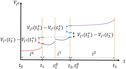
FIGURE 1. Conditions 1), 2) and 3) of Theorem 2 regarding the allowable changes in the values of the Lyapunov functions. The increments shown by blue, red and black double-arrows pertain to condition 1), 2) and 3), respectively.

• Note that since V_i’s are positive definite functions, there exists a class-$\mathcal{K}$ function α₀ such that V_i(x) ≤ α₀ (‖x‖) for all $x\in {\mathbb{R}}^n$ [see (Khalil and Grizzle, 2002, Lemma 4.3)].

• Condition 1) means that the cumulative value of the differences between the consecutive Lyapunov functions at the switching instants of the dynamics of continuous flows (i.e., at switches of the signal σ_f) is bounded by a class-$\mathcal{K}$ function. The functions are evaluated at the post-jump value of the state to include the case when a discrete-jump happens to occur at t = t_k+1. If there is no discrete-jump at t = t_k+1, then simply $V_{i^{k+1}}(x(t_{k+1}^{+}))-V_{i^k}(x(t_{k+1}^{+}))=V_{i^{k+1}}(x(t_{k+1}))-V_{i^k}(x(t_{k+1}))$.

• Condition 2) means that the cumulative increment in the values of the individual Lyapunov functions when the respective modes are active (evaluated before and after a discrete-jump at t_k+1 and t_k, respectively, if any) is bounded by a class-$\mathcal{K}$ function³

• Eq. 7 in condition 3) means that the cumulative increment in the value of the Lyapunov function V_i is bounded by a class-$\mathcal{K}$ function at the discrete jumps occurring at the switching instants, i.e., t_k+1 ∈ J_i. Condition Eq. 6 inherently accommodates any discrete jumps occurring in the interior of the time interval (t_k, t_k+1), i.e., in between two switching instants, for any mode i ≠ F. Thus, we only need to account for the discrete jumps occurring at the boundaries of these intervals through (7) [see, e.g., (Wang et al., 2018)].

• Condition 4) means that there exists an FTS mode F ∈Σ and a Lyapunov function V_F satisfying Eq. 2 for $x(t)=f_F(x(t))$ on $[t_{F_k},t_{F_k+1})\backslash J_F$ for all $k\in {\mathbb{Z}}_{+}$.

• Condition 5) means that the FTS mode F is active for a sufficiently long cumulative time γ(‖x₀‖) without any discrete jump occurring in that cumulative period.

Now we provide the proof of Theorem 2.

Proof. First we prove the stability of the origin under conditions (1–3). Let x₀ ∈ D, where D is some open neighborhood of the origin. For all $p\in {\mathbb{Z}}_{+}$, we have that

$\begin{array}{ll}\hfill V_{i^p}(x(t_p^{+}))& =V_{i^0}(x(t_0))+\sum _{k=1}^p\left(V_{i^k}(x(t_k^{+}))-V_{i^{k-1}}(x(t_k^{+}))\right)+\sum _{k=0}^{p-1}\left(V_{i^k}(x(t_{k+1}^{-}))-V_{i^k}(x(t_k^{+}))\right)\hfill \\ \hfill & +\sum _{i=1}^{N_f}\sum _{t\in J_i}\left(V_i(x(t^{+}))-V_{i^k}(x(t^{-}))\right)\hfill \\ \hfill & {\le }^{\left(5\right),\left(6\right),\left(7\right)}{\alpha }_0(\Vert x_0\Vert )+{\alpha }_1(\Vert x_0\Vert )+{\alpha }_2(\Vert x_0\Vert )+N_f{\alpha }_3(\Vert x_0\Vert )\hfill \\ \hfill & =\alpha (\Vert x_0\Vert )\hfill \end{array}$

where $\alpha ={\alpha }_0+{\alpha }_1+{\alpha }_2+N_f{\alpha }_3\in \mathcal{K}$ with ${\alpha }_0(r)=\underset{i\in {\mathrm{\Sigma }}_f,\Vert x\Vert \le r}{\max }{V}_i(x)$. Thus, we have:

$V_{i^p}(x(t_p^{+}))\le \alpha (\Vert x_0\Vert ),(9)$

for all $p\in {\mathbb{Z}}_{+}$. Let d_i (c) = {x | V_i(x) ≤ c} denote the c sub-level set of the Lyapunov function V_i, i ∈Σ_f, and B_ρ = {x | ‖x‖ ≤ ρ} denote a ball centered at the origin with radius $\rho \in {\mathbb{R}}_{+}$. Define r (c) = inf{ρ ≥ 0 | d_i(c) ⊂ B_ρ} as the radius of the smallest ball centered at the origin that encloses the c sub-level sets d_i (c), for all i ∈Σ_f.

Since the functions V_i are positive definite, the sub-level sets d_i (c) are bounded for small c > 0, and hence, the function r is invertible. The inverse function c_ϵ = r⁻¹ (ϵ) maps the radius ϵ > 0 to the value c_ϵ such that the sub-level sets d_i (c_ϵ) are contained in B_ϵ for all i ∈Σ_f. For any given ϵ > 0, choose δ such that α(δ) ≤ (r⁻¹ (ϵ)) > 0 so that Eq. 9 implies that for ‖x₀‖ ≤ δ, we have $V_{i^p}(x(t_p^{+}))\le \alpha (\Vert x_0\Vert )\le \alpha (\delta )\le r^{-1}(ϵ)$, which implies that $\Vert x(t_p^{+})\Vert \le ϵ$ for all $p\in {\mathbb{Z}}_{+}$, i.e., the origin is LS.

Next, we prove FTS of the origin when conditions (4–5) also hold. From Eq. 9, we have that

$V_F(x(t_{F_i}))\le \alpha (\Vert x_0\Vert ),(10)$

for all $i\in \mathbb{N}$. By definition, we have that there is no discrete jump during $T_{F_k}$, for all $k\in \mathbb{N}$. Let $M\in \mathbb{N}$ denote the total number of times the mode F is activated. From condition 4), we have

$V_F(x(t))\le -c{V}_F{(x(t))}^{\beta }.(11)$

for all $t\in \bigcup T_{F_k}\subset \left(\bigcup [t_{F_k},t_{F_k+1})\backslash J_F\right)$. Using the fact there is no discrete jump in $T_{F_k}$, we can integrate Eq. 11 to obtain $T_{F_k}|\le \frac{V_{F_k}^{1-\beta }}{c(1-\beta )}-\frac{V_{F_k+1}^{1-\beta }}{c(1-\beta )}$, where $|T_{F_k}|=t_{F_k+1}-t_{F_k}$. Thus, for any $M\in \mathbb{N}$, we have that

$\sum _{k=1}^M|T_{F_k}|\le \sum _{k=1}^M\left(\frac{V_{F_k}^{1-\beta }}{c(1-\beta )}-\frac{V_{F_k+1}^{1-\beta }}{c(1-\beta )}\right)=\frac{V_{F_1}^{1-\beta }}{c(1-\beta )}+\sum _{i=1}^{M-1}\frac{V_{F_{i+1}}^{1-\beta }-V_{F_i+1}^{1-\beta }}{c(1-\beta )}-\frac{V_{F_M+1}^{1-\beta }}{c(1-\beta )}.$

Using Eq. 10, we obtain that

$\frac{V_{F_1}^{1-\beta }}{c(1-\beta )}\le \frac{\alpha {(\Vert x_0\Vert )}^{1-\beta }}{c(1-\beta )}.(12)$

Define ${\gamma }_1(\Vert x_0\Vert )\triangleq \frac{{(\alpha (\Vert x_0\Vert ))}^{1-\beta }}{c(1-\beta )}$ and note that ${\gamma }_1\in \mathcal{K}$. Now, let Q = {q₁, q₂, … , q_k}, 0 ≤ q_l ≤ M, be the set of indices such that $V_{F_{i+1}}\ge V_{F_i+1}$ for i ∈ Q. We know that for a ≥ b ≥ 0, a^r ≥ b^r for any r > 0. Hence, we have that

$\sum _{i=1}^{M-1}\frac{V_{F_{i+1}}^{1-\beta }-V_{F_i+1}^{1-\beta }}{c(1-\beta )}\le \sum _{i\in Q}\frac{V_{F_{i+1}}^{1-\beta }-V_{F_i+1}^{1-\beta }}{c(1-\beta )}(13)$

Using Lemma 1, we obtain that

$\sum _{i\in Q}\frac{V_{F_{i+1}}^{1-\beta }-V_{F_i+1}^{1-\beta }}{c(1-\beta )}\le \sum _{i\in Q}\frac{{(V_{F_{i+1}}-V_{F_i+1})}^{1-\beta }}{c(1-\beta )}.(14)$

From the analysis in the first part of the proof, we know that V_F (x (t)) ≤ α (‖x₀‖). Define $\alpha =2M\alpha$ so that we have

$\sum _{i\in Q}\left(V_{F_{i+1}}-V_{F_i+1}\right)\le \sum _{i\in Q}\left(V_{F_{i+1}}+V_{F_i+1}\right)\le 2M\alpha (\Vert x_0\Vert )=\alpha (\Vert x_0\Vert ).(15)$

Hence, we have that

$\sum _{i=1}^{M-1}\frac{V_{F_{i+1}}^{1-\beta }-V_{F_i+1}^{1-\beta }}{c(1-\beta )}\stackrel{\left(14\right)}{\le }\frac{\sum _{i\in Q}{\left(V_{F_{i+1}}-V_{F_i+1}\right)}^{1-\beta }}{c(1-\beta )}\le \frac{M^{-\beta }{\left(\sum _{i\in Q}{V}_{F_{i+1}}-V_{F_i+1}\right)}^{1-\beta }}{c(1-\beta )}\stackrel{\left(15\right)}{\le }\frac{M^{-\beta }{(\alpha (\Vert x_0\Vert ))}^{1-\beta }}{c(1-\beta )},(16)$

where the second inequality follows from (Zuo and Tie, 2016, Lemma 3.4). Define $\gamma (\Vert x_0\Vert )\triangleq {\gamma }_1(\Vert x_0\Vert )+\frac{M^{-\beta }{(\alpha (\Vert x_0\Vert ))}^{1-\beta }}{c(1-\beta )}$ and $|T_F|={\sum }_{k=1}^M|T_{F_k}|$ so that we obtain:

$|T_F|+\frac{V_{F_M+1}^{1-\beta }}{c(1-\beta )}\le \frac{V_{F_1}^{1-\beta }}{c(1-\beta )}+\sum _{i=1}^{M-1}\frac{V_{F_{i+1}}^{1-\beta }-V_{F_i+1}^{1-\beta }}{c(1-\beta )}\le \gamma (\Vert x_0\Vert ).$

Clearly, $\gamma \in \mathcal{K}$. Now, with $|T_F|=\gamma (\Vert x_0\Vert )$, we obtain

$|T_F|+\frac{V_{F_M+1}^{1-\beta }}{c(1-\beta )}\le \gamma (\Vert x_0\Vert )=|T_F|,$

which implies that $\frac{V_{F_M+1}^{1-\beta }}{c(1-\beta )}\le 0$. However, $V_F\ge 0$, which further implies that $V_{F_M+1}=0$. Hence, if mode F is active for the accumulated time $|T_F|=\gamma (\Vert x_0\Vert )$ without any discrete jump in the system state, the value of the function V_F converges to 0 as $t\to t_{F_M+1}$, and thus, the origin of Eq. 4 is FTS. Finally, if all the conditions (1–5) hold globally and the functions V_i are radially unbounded, we have that α₀ is also radially unbounded and ${\alpha }_1,{\alpha }_2,{\alpha }_3\in {\mathcal{K}}_{\infty }$. Thus, we have that α(‖x₀‖) < ∞ and $\alpha (\Vert x_0\Vert )<\infty$ for all ‖x₀‖ < ∞, and hence, γ(‖x₀‖) < ∞ for all ‖x₀‖ < ∞, which implies global FTS of the origin.

Estimation of time of activation$|T_F|$: Note that the expression of $|T_F|$ in condition 5) of Theorem 2 depends on M, the number of times the mode F is activated. In practice, the number M might not be know beforehand. However, an upper bound on the cumulative time of activation $|T_F|$ can still be computed as follows. For the origin of the hybrid system Eq. 4 to be FTS, it is necessary that the mode F is active at least once. Furthermore, under the assumption that there is a dwell-time τ > 0 so that system solutions are non-Zeno, we know that $|T_{F_k}|\ge \tau$. Using these two arguments, we can find an upper bound on $|T_F|$ in Theorem 2. In particular, the upper bound is given as:

$|T_F|\le \max \left\{\frac{\alpha {(\Vert x_0\Vert )}^{1-\beta }}{c(1-\beta )}+\frac{2\alpha {(\Vert x_0\Vert )}^{1-\beta }}{c(1-\beta )},\lceil M^{*}\rceil {\tau }_F\right\}(17)$

where M* is the solution of

$\frac{\alpha {(\Vert x_0\Vert )}^{1-\beta }}{c(1-\beta )}+\frac{M^{1-2\beta }{2}^{1-\beta }\alpha {(\Vert x_0\Vert )}^{1-\beta }}{c(1-\beta )}=M{\tau }_F.(18)$

Activation of the FTS mode: Intuitively, Theorem 2 can be interpreted as follows: if Lyapunov stability of the origin can be established for a given switching signal σ_f, then the presence of a switching signal and an FTS mode such that the latter is active for a sufficient amount of time $|T_F(\Vert x_0\Vert )|$ without any discrete jump guarantees FTS of the origin for the overall system. Depending upon the application at hand, and available authority on the design of the switching signal, the FTS mode can be made active for the required cumulative duration in one activation period, or in multiple activation periods. For the cases when designing the switching signal is not under user’s control, it is possible that the dynamics switches between the FTS and the non-FTS modes, and in such a case, Theorem 2 guarantees FTS when the FTS mode is active for a sufficient amount of cumulative time.

Comparison with earlier results: In contrast to (Zhao and Hill, 2008, Proposition 3.8), where the authors provided necessary and sufficient conditions for stability of switched system under Eq. 9 and non-increasing condition on the Lyapunov functions V_i during activation period, we proved stability of the origin with just Eq. 9. Compared to Li and Sanfelice (2019), our results are less conservative in the sense that the Lyapunov functions are allowed to increase during the continuous flows (per Eq. 6), as well as at the discrete jumps (per Eq. 7). In other words, we allow unstable modes to be present in the hybrid system while still guaranteeing FTS of the origin.

A note on construction of functionsV_i: In practice, the conditions (1–3) in Theorem 2, or those presented in Zhao and Hill (2008) can be difficult to verify for a general class of hybrid systems involving non-linear subsystems. For a class of switched systems consisting of N − 1 linear modes and one FTS mode F, one can follow a procedure similar to (Zhao and Hill, 2008, Remark 3.21) to construct the functions μ_ij to design the switching signal σ_f, as well as the Lyapunov candidates V_i for i ≠ F. The design procedure includes choosing quadratic functions μ_ij = x^TP_ijx and V_i = x^TR_ix with R_i as positive definite matrices to formulate a linear matrix inequality (LMI) problem. For systems consisting of polynomial dynamics f_i, one can formulate a sum-of-square (SOS) problem to find polynomial functions V_i, μ_ij [see Parrilo (2000) for an overview of SOS programming and (Prajna et al., 2002) for methods of solving SOS problems]. The study of finding Lyapunov functions to assess stability for a general class of hybrid systems with nonlinear modes is an open field of research, and is out of scope of this work.

3 Simulations

We present an instance of the hybrid system Eq. 4 with five modes, where one mode is FTS, one is AS, and three are unstable. The simulation results have been obtained by discretizing the continuous-time dynamics using Euler discretization. We use a step size of dt = 10^–3, and run the simulations till the norm of the states drops below 10^–10. At this point we wish to emphasize that while the theoretical results hold for the continuous-time dynamics, and not for the implemented discretized dynamics, still the simulations reflect stable behavior that meets the theoretical bounds on the sufficiently long active time of the finite-time stable mode. Consider the hybrid system $\mathcal{H}=\{C,\mathcal{F},D,\mathcal{G}\}$ where

$\begin{array}{cc}\hfill & \mathcal{F}=\{f_1,f_2,f_3,f_4,f_5\},\mathcal{G}=\{g_1\},C=D={\mathbb{R}}^2,\hfill \\ \hfill & f_1=\left[\begin{array}{c}\hfill 0.01x_1^2+x_2\hfill \\ \hfill -0.01x_1^3+x_2\hfill \end{array}\right],f_2=\left[\begin{array}{c}\hfill 0.01x_1-x_2\hfill \\ \hfill -x_1^2+0.01x_2\hfill \end{array}\right],\hfill \\ \hfill & f_3=\left[\begin{array}{c}\hfill -x_1-x_2\hfill \\ \hfill x_1-x_2\hfill \end{array}\right],f_4=\left[\begin{array}{c}\hfill 0.01x_1^2+0.01x_1{x}_2\hfill \\ \hfill -0.01x_1^3+x_2^2\hfill \end{array}\right],\hfill \\ \hfill & f_5=\left[\begin{array}{c}\hfill x_2-20\mathrm{sign}(x_1)|x_1{|}^{\beta }\hfill \\ \hfill -10\mathrm{sign}(x_1)|x_1{|}^{2-2\beta }\hfill \end{array}\right],g_1=\left[\begin{array}{c}\hfill -1.1x_1\hfill \\ \hfill -1.1x_2\hfill \end{array}\right],\hfill \end{array}(19)$

with β = 0.98, where the fifth mode is FTS, and thus F = 5. Note that the states x₁ and x₂ change sign and increase in magnitude at the discrete jumps. The Lyapunov functions are defined as V_i(x) = x^TP_ix, for i ∈{1, 2, 3, 4}, with $P_1=\left[\begin{array}{cc}\hfill 1\hfill & \hfill 0\hfill \\ \hfill 0\hfill & \hfill 1\hfill \end{array}\right],P_2=\left[\begin{array}{cc}\hfill 5\hfill & \hfill 2\hfill \\ \hfill 2\hfill & \hfill 4\hfill \end{array}\right],P_3=\left[\begin{array}{cc}\hfill 1\hfill & \hfill 0\hfill \\ \hfill 0\hfill & \hfill 3\hfill \end{array}\right],P_4=\left[\begin{array}{cc}\hfill 6\hfill & \hfill 1\hfill \\ \hfill 1\hfill & \hfill 3\hfill \end{array}\right]$, and $V_5(x)=\frac{5}{\beta }|x_1{|}^{2\beta }+\frac{1}{2}|x_2{|}^2$. Note that this example is more general than the examples considered in (Li and Sanfelice, 2019), as we allow the dynamics to have unstable modes. In this example, the switches in the continuous flows occur after 0.2 sec, i.e., $|T_{i_k}|=0.2$ sec, $k\in {\mathbb{Z}}_{+}$, and discrete jumps occur after 0.1 s for all i ∈{1, 2, … , 5}.

The switching signal is designed so that the Lyapunov candidates V_i satisfy conditions 1) and 3) of Theorem 2 (see Garg and Panagou, 2021) for a discussion on how a finite-time stabilizing switching signal can be designed). Mode 3 and 5, being stable, satisfy condition 2) with α₂ = 0, and modes 1, 2 and 4, being active for a finite interval each time, satisfy condition 2) with α₂ = k‖x₀‖² for some k > 0, and so α₂ = k‖x₀‖² satisfy 2) for all the modes. It can be verified that f₅ is homogeneous with degree of homogeneity d = α − 1 < 0. Thus, using (Bhat and Bernstein, 2005, Theorem 7.2), the origin is FTS under the system dynamics f₅, and there exists a V₅ satisfying Eq. 8; therefore, condition 4) is satisfied. Finally, the switching signal is designed so that mode five is active for a sufficient amount of time that satisfies condition 5).

Figure 2 illustrates the state trajectories x₁ (t) and x₂ (t). Note that the states change sign at the discrete jumps. Figure 3 depicts the norm of the state vector x (t) on log scale; note that ‖x (t)‖ is increasing while operating in unstable modes, and decreasing while operating in stable modes. As seen in the figures, the system states, starting from ‖x (0)‖ = 10, reach to a norm of ‖x (t)‖ ≤ 10^–10 within first 90 s of the simulation. Finally, Figure 4 illustrates the evolution of the Lyapunov functions V_i with respect to time; note that the Lyapunov functions increase, as expected, at the times of the switches in σ_f, as well as during the continuous flows along the unstable modes 1, 2, and 4. The provided example demonstrates that the origin of the system is FTS even when one or more modes are unstable, if the FTS mode is active for a sufficient amount of time.

FIGURE 2

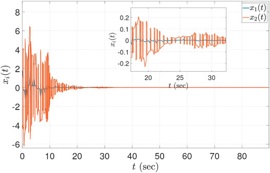
FIGURE 2. The evolution of x₁ (t) and x₂ (t) for hybrid system Eq. 19. The states can be seen switching signs during discrete jumps.

FIGURE 3

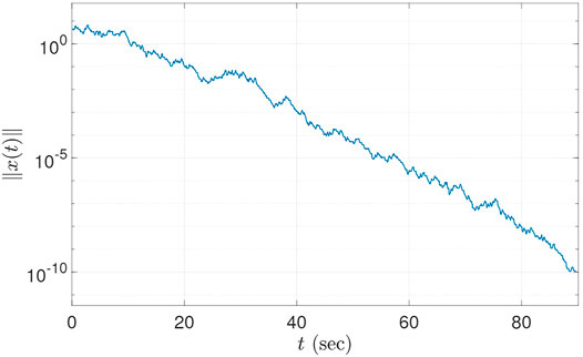
FIGURE 3. The evolution of ‖x (t)‖ for Eq. 19. The norm of the states reach a small neighborhood of the origin within a finite time.

FIGURE 4

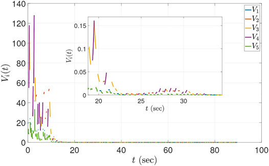
FIGURE 4. The evolution of the Lyapunov functions V_i (t) for t ∈ (0, 10) sec for Eq. 19. The Lyapunov functions for unstable modes (mode 2 and 4) increase when the respective modes are active.

4 Conclusions and Future Work

In this paper, we studied FTS of a class of hybrid systems. We showed that under some mild conditions on the bounds of the increase of the Lyapunov functions, if the FTS mode is active for a sufficient cumulative time, then the origin of the hybrid system is FTS. Our proposed method allows the individual Lyapunov functions to increase both during the continuous flows as well as at the discrete state jumps, i.e., it allows the hybrid system to have unstable modes.

Future research focuses on incorporating input and state constraints in the hybrid systems framework to model safety (in the sense of invariance of a safe set of states) and temporal requirements (in the sense of convergence to a set or to a point within an arbitrarily chosen time, if possible). More specifically, we would like to investigate how to impose convergence of the system trajectories in a finite time that can be a priori selected independent of the initial conditions, so that the overall framework can be used for the synthesis and analysis of controllers under spatiotemporal specifications.

Data Availability Statement

The original contributions presented in the study are included in the article/Supplementary Material, further inquiries can be directed to the corresponding author.

Author Contributions

KG is responsible for the conceptualization, the simulation and the writing of this paper. DP is responsible for the funding acquisition, the conceptualization of the main idea and the revisions of the paper.

Funding

The authors would like to acknowledge the support of the Air Force Office of Scientific Research under award number FA9550-17-1-0284.

Conflict of Interest

The authors declare that the research was conducted in the absence of any commercial or financial relationships that could be construed as a potential conflict of interest.

Publisher’s Note

All claims expressed in this article are solely those of the authors and do not necessarily represent those of their affiliated organizations, or those of the publisher, the editors and the reviewers. Any product that may be evaluated in this article, or claim that may be made by its manufacturer, is not guaranteed or endorsed by the publisher.

Footnotes

¹With slight abuse of notation, we use FTS to denote the phrase “finite-time stability” or “finite-time stable”, depending on the context.

²A sufficient condition for the solutions of a switched or hybrid to exhibit non-Zeno behavior is that there is a non-zero dwell-time τ > 0 between any two switching instants [see (Liberzon, 2003)].

³Note that some authors use the time derivative condition, i.e., $\dot{V}_{i}\leq {\lambda} V_{i}$ with λ > 0, in place of condition 2), to allow growth of Vi, hence, requiring each Vi to be continuously differentiable.

References

Bhat, S. P., and Bernstein, D. S. (2000). Finite-time stability of continuous autonomous systems. SIAM J. Control. Optim. 38, 751–766. doi:10.1137/s0363012997321358

CrossRef Full Text | Google Scholar

Bhat, S. P., and Bernstein, D. S. (2005). Geometric homogeneity with applications to finite-time stability. Math. Control. Signals Syst. 17, 101–127. doi:10.1007/s00498-005-0151-x

CrossRef Full Text | Google Scholar

Branicky, M. S. (1998). Multiple Lyapunov functions and other analysis tools for switched and hybrid systems. IEEE Trans. Automat. Contr. 43, 475–482. doi:10.1109/9.664150

CrossRef Full Text | Google Scholar

Fu, J., Ma, R., and Chai, T. (2015). Global finite-time stabilization of a class of switched nonlinear systems with the powers of positive odd rational numbers. Automatica 54, 360–373. doi:10.1016/j.automatica.2015.02.023

CrossRef Full Text | Google Scholar

Garg, K., and Panagou, D. (2021). Finite-time stabilization of switched systems with unstable modes. IEEE Conference on Decision and Control. Submitted, under review (IEEE).

Goebel, R., Sanfelice, R. G., and Teel, A. R. (2012). Hybrid Dynamical Systems: Modeling, Stability, and Robustness. Princeton, New Jersey: Princeton University Press.

Khalil, H. K., and Grizzle, J. W. (2002). Nonlinear Systems, Vol. 3. Upper Saddle River, NJ): Prentice hall.

Li, Y., and Sanfelice, R. G. (2019). Finite time stability of sets for hybrid dynamical systems. Automatica 100, 200–211. doi:10.1016/j.automatica.2018.10.016

CrossRef Full Text | Google Scholar

Liberzon, D. (2003). Switching in Systems and Control. Germany: Springer Science & Business Media.

Lin, H., and Antsaklis, P. J. (2009). Stability and stabilizability of switched linear systems: a survey of recent results. IEEE Trans. Automat. Contr. 54, 308–322. doi:10.1109/tac.2008.2012009

CrossRef Full Text | Google Scholar

Liu, X., Ho, D. W. C., Song, Q., and Cao, J. (2017). Finite-/fixed-time robust stabilization of switched discontinuous systems with disturbances. Nonlinear Dyn. 90, 2057–2068. doi:10.1007/s11071-017-3782-9

CrossRef Full Text | Google Scholar

Parrilo, P. A. (2000). Structured semidefinite programs and semialgebraic geometry methods in robustness and optimization. California: California Institute of Technology (Ph.D. thesis.

Peleties, P., and DeCarlo, R. (1991). Asymptotic stability of m-switched systems using lyapunov-like functions, 1991 American Control Conference (IEEE). 1679–1684. doi:10.23919/acc.1991.4791667

CrossRef Full Text

Prajna, S., Papachristodoulou, A., and Parrilo, P. A. (2002). Introducing SOSTOOLS: a general purpose sum of squares programming solver, 41st IEEE Conference on Decision and Control (IEEE). 741–746.

Ríos, H., Davila, J., and Fridman, L. (2015). “State estimation on switching systems via high-order sliding modes,” in Hybrid Dynamical Systems (Germany: Springer), 151–178. doi:10.1007/978-3-319-10795-0_6

CrossRef Full Text | Google Scholar

Ryan, E. (1991). “Finite-time stabilization of uncertain nonlinear planar systems,” in Mechanics and Control (Germany: Springer), 406–414. doi:10.1007/bf02169426

CrossRef Full Text | Google Scholar

Sanfelice, R. G., Goebel, R., and Teel, A. R. (2007). Invariance principles for hybrid systems with connections to detectability and asymptotic stability. IEEE Trans. Automat. Contr. 52, 2282–2297. doi:10.1109/tac.2007.910684

CrossRef Full Text | Google Scholar

Wang, Y.-E., Karimi, H. R., and Wu, D. (2018). “Conditions for the stability of switched systems containing unstable subsystems,” in IEEE Transactions on Circuits and Systems II: Express Briefs. IEEE.

Google Scholar

Zhang, B. (2018). On finite-time stability of switched systems with hybrid homogeneous degrees. Math. Probl. Eng. 2018, 1–7. doi:10.1155/2018/309698610.1155/2018/3096986

CrossRef Full Text | Google Scholar

Zhao, J., and Hill, D. J. (2008). On stability, l₂-gain and H_∞ control for switched systems. Automatica 44, 1220–1232. doi:10.1016/j.automatica.2008.05.010

CrossRef Full Text | Google Scholar

Zhao, X., Zhang, L., Shi, P., and Liu, M. (2012). Stability of switched positive linear systems with average dwell time switching. Automatica 48, 1132–1137. doi:10.1016/j.automatica.2012.03.008

CrossRef Full Text | Google Scholar

Zuo, Z., and Tie, L. (2016). Distributed robust finite-time nonlinear consensus protocols for multi-agent systems. Int. J. Syst. Sci. 47, 1366–1375. doi:10.1080/00207721.2014.925608

CrossRef Full Text | Google Scholar