Resilient Biomedical Systems Design Under Noise Using Logic-Based Machine Learning

1 Introduction

The introduction of machine learning (ML) in healthcare has already shown promise in automated diagnosis (Alaoui et al., 2021), most notably in mammogram abnormality detection (Amrane et al., 2018). Its use is likely to expand in other diseases with more exploration into new detection methods, enabled by advances in sensing technologies, coupled with high-throughput computing architectures (Alizadehsani et al., 2021; Baldi, 2018). The rise of this big data landscape has led to an industry-wide reliance on electronic health records (Driggs et al., 2021). Therefore, it is expected that close-knit integration of AI into clinical decision support systems will lead to greater personalization with fast yet reliable diagnosis to tackle the forecast population increase (Castiglioni et al., 2021).

Nevertheless, there remains the possibility of noise corruption in data collection methods which may propagate through an ML diagnosis pipeline resulting in uncertainty or an incorrect classification. This is seen when a feature is blemished through a fluctuation from the nominal value; this new value may then play a crucial part in the classifier deciding the class boundaries. If the range of values that the feature can take is close together, then the effects that are intensified as class boundaries can become less distinct (Shathini et al., 2019). Traditional approaches of mitigating the impact of noise, such as the incorporation of error correction codes or redundancy methods, can incur significant costs in terms of model complexity, learning convergence time, memory requirements, and performance degradation (Gupta and Gupta, 2019).

Naturally, it is understandable why noise corruption may arise when looking into the general characteristics of biomedical data, the main factor being data heterogeneity (Baldi, 2018). Medical data can span many orders of magnitude with specific spatial and temporal characteristics of interest, and it can also range from analog, digital, text, or complex data structures such as sequences or trees. Often the data will come from several sources and may not have a uniform structure; in many cases with clinical data, data imputation techniques are needed to fill missing value gaps, but overuse of this will lead to inaccurate analysis or incorrect conclusions (Tice and Farag, 2019).

To address these problems there are two routes for reducing noise effects for ML applications: a) focusing on data quantity, integrity, and representation granularity (often tackled at the preprocessing stage) and b) the ML models’ learning ability when data points are small.

Gathering sufficient training data to represent the problem is a logical technique to diminish the effects of outlier points in the models’ classification (Driggs et al., 2021), albeit the “small-data” problem is difficult to address for certain medical applications where the disease or virus is novel. However, to tackle this issue for known diseases in classical machine learning pipelines, it is better to create curated data sets where medical experts have removed outlier features (Thottakkara et al., 2016; Castiglioni et al., 2021) or to use techniques such as regularization and other data augmentation techniques to create a more defined problem space (Tice and Farag, 2019). But the method of hand-crafted feature extraction has obvious drawbacks when considering the scale with which future medical data machine learning must be designed for. Data with higher dimensionality will require more time to analyze and curate; in addition, most ML problems are data hungry and will require many data points to leverage satisfactory performance (Obermeyer and Emanuel, 2016).

In traditional machine learning systems, such as neural networks, arithmetic processes can be used to filter out some effects of the noise from the expanded data. This may include adding extra convolution processes to adding more noise screening neural layers (Sukhbaatar and Fergus, 2014). This additional complexity can often be quite significant and may require a system-wide hyperparameter optimization for performance and compact representation (Cao et al., 2020).

To this end, it is better to focus on the second route, adjusting the ML to learn the key information for the “small-data” and reduce uncertainty. According to Gal (2016), the model uncertainty can be seen through two types: model structure uncertainty and model parameter uncertainty; both of which are grouped together and referred as epistemic uncertainty. Therefore one of the main indicators of robustness to noise should be a minimal effect of this uncertainty on the ML model.

In this study, we examine the problem of noise corruption into medical data with the outlook of creating preprocessing and ML methods for noise resilience. We are particularly interested in investigating the impact of noise on a new, logic-driven ML algorithm called the Tsetlin machine (Granmo, 2021). We examine the different ways in which noise can be injected into training and testing data and focus on ways in which the feature spaces of these data sets can be reduced as much as possible while mitigating the impact of noise. We do this with both the intention of examining how ML might be resilient when using data from noise-corrupted electronic health records and also with the aim of minimizing model complexity and energy expenditure. Through these insights we explore the possibilities of edge ML for medical data. We introduce the data sets that will be used and then present the specific contributions and overview of this study.

1.1 Data sets Used for Noise Injection

To evaluate the impact of noise we chose three data sets with specific qualities that might effect our preprocessing method when paired with the Tsetlin machine. We measure performance in terms of sensitivity and specificity, and the TM’s convergence efficiency is expressed in terms of Nash equilibrium. The data sets are as follows:

• Breast Cancer: A data set developed by Dr. William H. Wolberg from patients attended between January 1989 and November 1991 at the University of Wisconsin Hospitals. Wolberg states three crucial aspects for diagnostic decision making for this data set: the universality of the data used in the training set, precision of the numerical representations of the features, and the inherent mutual exclusiveness of the two classes—see Wolberg and Mangasarian (1990). The classification for the Breast Cancer data set is the determination of benign and malignant tumors based on the floating point mammogram data from cell samples taken from a patient. The floating point features represent cell properties such as radius, texture, and concavity. The objective of the TM is to create logic propositions that will determine the boundaries for each of these features that determine either malignant or benign diagnosis.

• Pima Indians Diabetes: This data set is from the National Institute of Diabetes and Digestive and Kidney Diseases. It consists of an oral glucose tolerance test (GTT) and general health measurements used to determine diabetes diagnosis of female Pima Indian population from Phoenix, Arizona. Schulz et al. (2006) states that malignant diagnoses are usually a combination of genetic attributes with environmental factors (not explicitly present in the data set). The data set contains challenges from the classification perspective as some features such as age and glucose levels do not follow normal distributions across the data points and may require more intelligent discretization in preprocessing. The classification of the Pima Indians Diabetes data set is the determination of whether a patient is diabetic based on blood pressure, age, insulin levels, etc. Once again the TM must create propositions that will form boundaries for these features to enable classification.

• Parkinson’s disease: This data set was created as a collaboration between the National Center of Voice and Speech and the University of Oxford to understand the relationship between the severity of Parkinson’s disease (PD) from speech signals. The data set contains 195 voice recordings from 31 people, 23 of whom have PD. The classification of Parkinson’s disease uses vocal recordings to determine the Parkinson’s diagnosis. The features here are different frequency measures and vocal jitter measures. Once again the TM must create propositions that will determine both which feature(s) and what empirical value they must have for Parkinson’s diagnosis.

These data sets will allow us to focus on some commonly faced challenges in medical data ML: the high dimensionality problem where not all features may have meaningful contributions to classification and the class imbalance problem which will dictate the number of false positives and false negatives in the classification depending on which class has more instances (Shanab et al., 2012).

1.2 Contributions

Through this study, we show how the Tsetlin machine is robust to noise impact when the SNR of the data set is reduced, we explore how feature extraction methods can aid the TM to offer better performance at low SNRs and how these extraction methods are themselves affected by noise injection, and finally, we explore the Nash equilibrium of Tsetlin machine’s model parameters to understand the impact of noise on parameter uncertainty. The main contributions are as follows:

• Evaluating the effect of adding attribute noise to the three data sets in question and empirically evaluating how this effect is propagated through the proposed preprocessing + TM pipeline and analyzed through the performance characteristics.

• Proposal of a new discretization and rule mining method for encoding data for the Tsetlin machine and exploration into the performance and noise resilience of this new technique when compared to the standard “Fixed Thresholding” approach to encoding data.

• Exploration into the classification capability of the Tsetlin machine in terms of accuracy, sensitivity, and specificity at varying SNRs when injecting noise into both training and testing data sets.

• Comparison of the Tsetlin machine with binary neural networks to test the robustness of these two different learning systems when injecting noise into training data set.

• Examining the possible energy expenditure of noise resilient TMs as edge nodes.

1.3 Article Outline

The structure of this article is as follows: Section 2 explores previous works that investigate noise injection into biomedical data to understand how commonly used ML models are effected as well as how certain preprocessing methods can be used to mitigate these noise effects. Section 3 introduces the ML model used to test robustness and explains the feature extraction methods employed to diminish noise impact. Section 4 describes the method for noise injection and discusses the testing methods for robustness using both training and testing data sets. The following sections show the experimental results of different noise injection procedures with emphasis on performance and ML models’ ability to cope with epistemic uncertainty.

2 Related Works

There are two different types of noise that can affect an ML model: attribute noise and class noise. Class noise may occur from subjectivity in the data or inadequate information being available for clear labeling (Pechenizkiy et al., 2006). Many neural network (NN)–based models have been explored with the aim of reducing class noise; Sukhbaatar and Fergus (2014) have shown that it is possible to learn from noisy labels using deep neural networks (DNNs) by adding an additional noise layer in the network that uses weights for this layer to learn noise distribution from the data. This method showed promising results on CIFAR10 with a 30% test error from training on 30k noisy training data points.

This method of adding an additional layer is also seen in Cao et al. (2020) where they incorporate a double soft-max design to counter overfitting due to noisy labels. This is done working on the principle suggested in Han et al. (2018) that deep learning models first memorize the clean data labels and then start to learn the noisy labels. The double soft-max design increases the training speed such that more time is spent learning the clean data labels.

Feature extraction methods such as principal component analysis have been effective in spreading out into new extracted axes based on the level of variability; while this is useful in unsupervised learning approaches and an effective form of dimensionality reduction, there is no guarantee that noise-corrupted features (or indeed discriminatory features for classification) will be present on the new axes (Pechenizkiy et al., 2006). This is shown by Romero (2010) on noisy ECG data, where the correlation coefficient starts to decrease as the SNR starts to decrease from 10dB to −10dB and the system variance increases and standard PCA helps in simplifying the problem space. To address this problem, Bailey (2012) proposed a method to weight the input data with known measurement error estimates, although this the method can be resilient to both measurement noise and missing values. This method can be useful with spectral data and systems where the measurement errors of the sensors are known; however, it still suffers from the fundamental issue with PCA. PCA works well when the correlations between feature points are linear; non-linear relations as seen with rotational changes in image data or time shifts in audio data are not correlated leading to more complex problem spaces for the ML to solve. The use of PCA as a preprocessing method with the Tsetlin machine has already been explored in Wheeldon et al. (2020); this method highlighted the benefits of PCA in dimensionality reduction but also poor scalability of larger data sets and data sets with class overlap.

When injecting Gaussian noise into gyroscopic and accelerometer data used to determine a person’s walking speed, Schooltink (2020) showed that upon injecting noise to this training data, it was only at around 60% noise percentage (noise to data) that the support vector classifier (SVC) and random forest start experiencing a major degradation in performance on the training data set.

In ensemble learning, methods such as vote-boosting have been effective in reducing noise by weighting the training data and removing unusually high weights; however, for ensemble learning, many instances of the classifier are required which poses issues of increasing memory and computing expense as the problem scales (Sabzevari et al., 2018).

Our method is designed to reduce the effects of attribute noise where erroneous values occur in one or more feature channels in the data set. We chose to focus on this problem as there are very few methods that explore reducing the effects of attribute noise, mainly due to the complexity of the problem (Gupta and Gupta, 2019). We explored three different routes to attribute noise injection: injecting specific feature channels, injecting all the features of the testing data, and injecting all the feature columns of the training data.

3 Tsetlin Machine

The Tsetlin machine (TM) is a recently proposed ML algorithm that incorporates the use of parallel state machines, such as learning automata, called Tsetlin automata (TA) to form propositional logic; this logic is used to form the relationships that describe the inputs to the determined classification (Granmo, 2021). The block diagram for the TM is given in Figure 1. In this section, we have provided an overview of the Tsetlin machine but readers are encouraged to refer to Granmo (2021); Abeyrathna et al. (2020); Granmo et al. (2019); Jiao et al. (2021) for detailed insights into TM’s functionality and proof of convergence, performance on commonly benchmarked data sets, and recent developments to the algorithm.

FIGURE 1

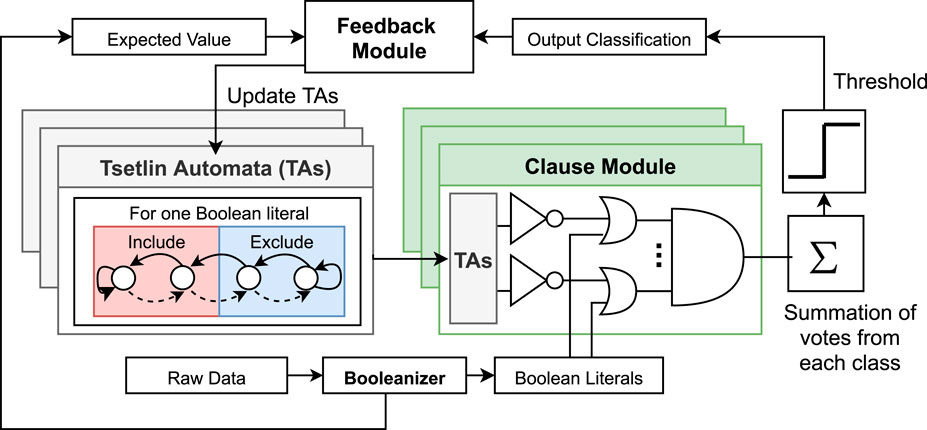
FIGURE 1. Block diagram of the Tsetlin machine.

Figure 1 shows that raw data must pass through a Booleanizer in order to be used by the TM. Booleanization is the encoding of a real value number to either 1 or 0. This is because the TM requires Boolean input features. Here, we have created a distinction between Booleanization and Binarization. For Boolean inputs, each individual bit has equal significance. The notion of a place value is not present unlike in binary and decimal numbering systems.

The next stage of the diagram is the transformation of the Boolean features into Boolean literals. Literals are formed by considering the Boolean feature and its negated form. The TM then creates a TA for each of these literals. In this way, we have an automata for every possible value the Boolean input can take. The TAs themselves correspond to two decisions based on which state the automata is in, include a literal or exclude a literal (view the Tsetlin automata).

The TAs are then used in the Clause Module which performs the operation shown in the block in Figure 1 to relate the include/exclude decisions of the TAs to the input literals. The clauses are stochastically independent blocks that form propositional logic and output a 1-bit value. The outputs of each clause are summed for each class, and the class with the most votes becomes the output classification. This decision is then given to the Feedback Module which updates each TA with a reward or penalty to transition its state.

Therefore, when the training process is complete and these TA states are fixed, we can perform simple logic operations that generate the output class—leading to explainable and dependable AI seen at the hardware level (Shafik et al., 2020). The Boolean data inputs also mean that bit-wise operations can be used over arithmetically heavy floating point computations; therefore, this linear logic–based structure allows for low energy expenditure in hardware implementations (Wheeldon et al., 2020, 2021).

Previous works has already shown that compared to NN methods, it is possible to create TMs with far fewer training parameters and much lower model complexity (Lei et al., 2021, 2020). This is further possible by creating minimal input Boolean feature spaces. In the next section, we have shown how this will impact the memory footprint, model complexity, and performance of the TM.

3.1 Feature Extraction Methods

The Tsetlin machine requires Boolean data as its inputs; this differs from binary data as all the bit inputs to the TM have equal significance. As seen through the diagram, the size of the TM is dictated by the number of inputs and the number of clauses. Therefore, to create smaller TM models that still offer high performance, there must be significant effort given to the preprocessing stage of transforming the raw features to Boolean features.

We have also seen that the number of TAs that are required is directly proportional to the number of inputs (number of TAs = number of clauses × number of classes × number of features × 2). Therefore, reducing the Boolean input space may dramatically reduce the memory footprint, the model complexity, and the number of clause operations that need to be performed. Smaller TMs will require fewer training parameters and perform inference quicker at a lower energy cost.

In this study, we have explored two routes to Booleanization of raw features as our key approaches of feature engineering. First, we have used Fixed Thresholding to Booleanize the data according to some predefined thresholds equally distributed across the feature columns; this is shown visually in Figure 2. Fixed thresholding is the current go-to method for Booleanizing data for the Tsetlin machine; it is favored because it is a simple algorithm that is portable to many problems. However, this method is unable to capture the skew in feature columns as it will simply equally distribute across the range of the highest and lowest values in the feature column. Therefore, we have also considered a method more statistically aware of the feature column distribution in the form of quantile binning. When dividing the features into bins, the bin number must be determined beforehand through a trial and error–based initial exploration.

FIGURE 2

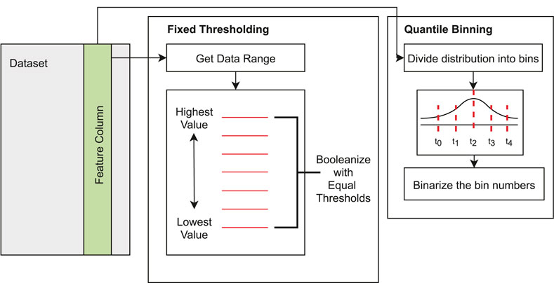
FIGURE 2. Visual representation fixed thresholding vs. quantile binning for data Booleanization.

The quantile binning method uses each feature column’s distributions to generate the bins giving a discretized representation of the feature space. These bin numbers are then binarized. These binary numbers then form the inputs to the Espresso logic minimizer algorithm (Brayton et al., 1984). Espresso combines minimization techniques presented by Quine (1952) and McCluskey Jr (1956) to create a set of sum of products (SoP) expressions for Boolean features that cannot be simplified any further. The full workflow for our proposed preprocessing method is shown in Figure 3. After the end of the pipeline, we have created a reduced Boolean data set for the training data and the testing data. For the testing data, we do not need to run the quantile binning or the minimizer, we simply used the quantiles found during the training and eliminated the redundant columns not used by the minimizer.

FIGURE 3

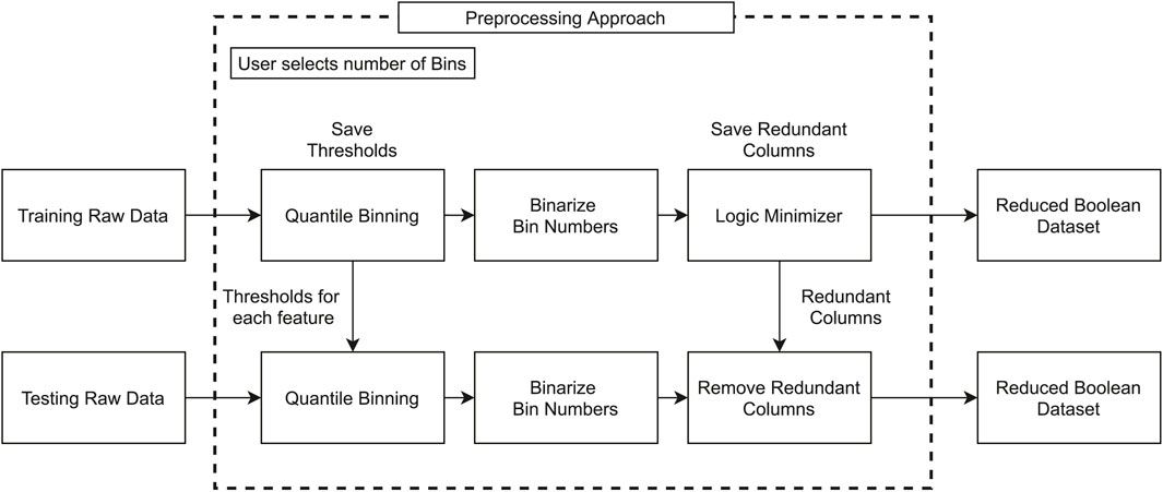
FIGURE 3. Visual representation of the full preprocessing workflow for training and testing data.

We propose this new method of Booleanization (Quantile binning + Espresso) to create a synergy between the Boolean inputs and the Tsetlin machine. We can use the quantile binning as a design knob for controlling the discretization level of the data, that is, the feature granularity. Then using the Espresso algorithm, the rule set of the Boolean feature set post-binning can be derived, thus enabling us to remove redundancies from the data and create a more condensed discriminatory data set for the TM.

Using logic minimization such as Espresso has been a common practice in built-in self-test (BIST) applications for many years (Galivanche and Reddy, 1987); however, given the Boolean inputs to the Tsetlin machine, it seems intuitive that using logic minimization would be an effective dimensionality reduction method. We present visual representation of how the logic minimizer works in Figure 4. We fed the initial Boolean space to the minimizer where each data point forms a logical AND expression relating to the resulting class. Using the minimizer, we can then form a condensed set of Boolean features that form the rule set for the TM. We can then eliminate feature columns that are not present in this rule set thus resulting in a smaller data set.

FIGURE 4

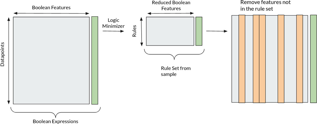
FIGURE 4. Visual representation of logic minimization on a data set.

4 Noise Injection Methods

To inject noise into the data sets chosen, we explored three main routes: injection into all elements of the testing data, injection in specific features of the testing data, and injection to the training data. All these methods require that the data set as a whole, or, the selected features injected with noise has a specific signal-to-noise ratio (SNR). Figure 5 shows how this is implemented.

FIGURE 5

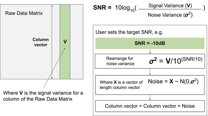
FIGURE 5. Injecting noise at a specific SNR.

For a particular feature of the data set matrix, we selected a particular SNR. Through this SNR we can derive the noise variance to inject for this particular feature. We used a Gaussian distribution across a vector of the same length of the target feature column to generate the noise values. Finally, vector addition of the target feature column vector with the noise vector gives the noise-injected data. We did this for both selected features (to inject noise to specific feature columns) and all features (to inject noise to all the feature columns) of the raw data matrix.

Figure 6 shows the full pipeline of injecting noise. We separated the data into testing and training data and applied the noise injection method shown in Figure 5 on specific features. The noise injection process happens in the preprocessing. We applied noise to the data before the quantile binning stage; this can happen for either the training or testing data based on the approach given in Figure 6. Using the noise injection technique expressed in Figure 6, we applied the three scenarios to explore the noise resilience of the TM. The most logical scenario is that the TM will be trained using clean data and tested on noisy data; however, we also evaluated the TM with both noisy training and testing data, this way we can also examine the epistemic uncertainty in the TAs when training on noisy data.

FIGURE 6

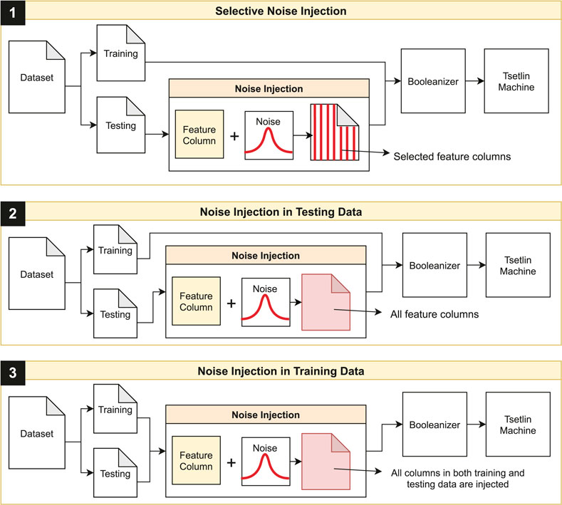
FIGURE 6. Workflow showing injection of noise to specific feature columns, all feature columns for the testing data, and all feature columns for both the testing and training data.

For quantifying noise impact, we explored the performance change through three indicators: classification accuracy, sensitivity, and specificity. Sensitivity and specificity are incredibly important performance measures for medical data as they offer greater insights into the classification ability in terms of true positives (TN), true negatives (TN), false positives (FP), and false negatives (FN). We have given a definition of sensitivity and specificity below:

$Sensitivity=\frac{TP}{TP+FN}(1)$

$Specificity=\frac{TN}{TN+FP}(2)$

5 Impact of Selective Noise Injection

Figure 7 shows the performance change as the SNR increases from −15 to 15dB when injecting specific columns of the Breast Cancer testing data with those SNRs. Given the skew of data points favoring the Benign class, it is expected that the specificity performance would be higher compared to the sensitivity, given there are fewer Malignant class instances. This is seen in the high specificity maintained throughout the SNR sweep.

FIGURE 7

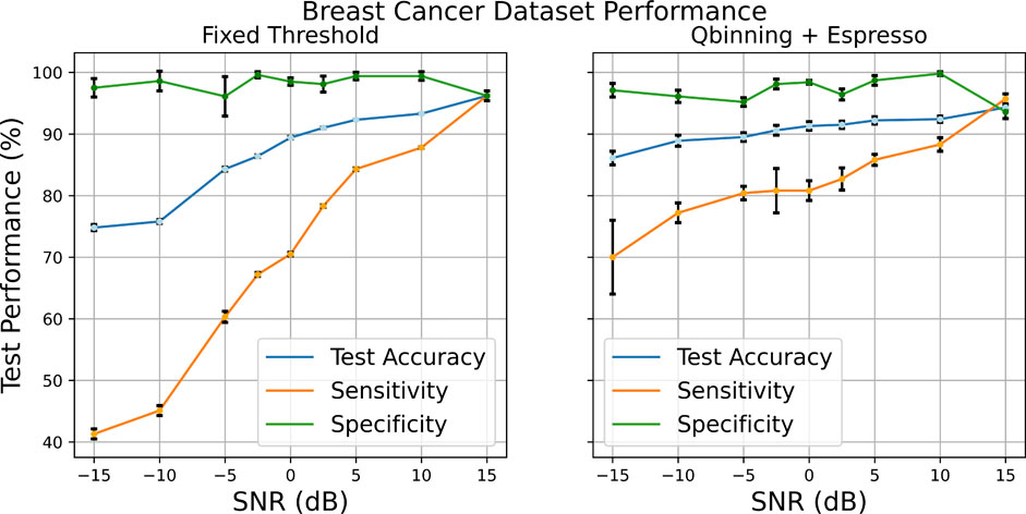
FIGURE 7. Comparison of the two different feature Booleanization methods when injecting specific feature columns of the testing data with noise.

The performance of the fixed threshold Booleanization is much poorer at low SNRs compared to that of the quantile binning + Espresso as seen through the sensitivity. For this experiment, the raw data was Booleanized with 10 bits used to represent each feature, resulting in 300 Boolean features altogether using the fixed thresholding method, while using quantile binning, 10 bins were used to discretize the features, resulting in a 4-bit representation per feature. Espresso then further reduced the feature space down; on average, the feature space was 45 features across the SNR sweep, as summarized in Table 1. The removal of these redundancies is possible through the rule mining approach of the Espresso minimizer; the features that are not present in the rule set are removed thus resulting in a smaller data set (as shown with Figure 4). Therefore, with significantly fewer features, we were able to produce a much more robust encoding method at low SNRs with equal performance at high SNRs.

TABLE 1

TABLE 1. Booleanization configuration for the Breast Cancer data set, with 100 clauses per class.

The large variance in sensitivity seen across the SNR sweeps of both fixed thresholding and Qbinning + Espresso is down to the class imbalance. With fewer data points corresponding to the Malignant class, it is more difficult to create a universal proportional logic in the training set that can then be used for testing. This is particularly true when certain Boolean features of the Malignant class have deviated away from the expected range due to the noise injection. For both preprocessing methods, it is clear that as the noise injection level is reduced (increasing SNR) the possible range a noise-injected feature can take is also reduced, thereby reflecting the features seen in the training set, and this leads to the increase in performance.To explore why the Quantile binning + Espresso method is superior at low SNRs, we looked deeper into the workflow, Figure 8. The block diagram flow at the top of the figure shows our general method; we injected noise into the target features and then performed the quantile binning and allocated the appropriate binary space to represent the binarized bin numbers. Note that, in the diagram, we have chosen to use eight bins for the quantile binning, this means that for each feature column data is divided into eight bins. We have represented the raw data as the binary bin number it is allocated to because there are eight bins and we need 3 bits to represent it. In Figure 8, we have shown this as the Boolean columns. Each feature column that we had at the start is now 3 Boolean columns (created by the 3-bit feature representation through binning; see the three spaces in the Boolean columns). After this point, each column has equal significance, that is, the notion of the place value is gone, and this is why we referred to them as Boolean columns.

FIGURE 8

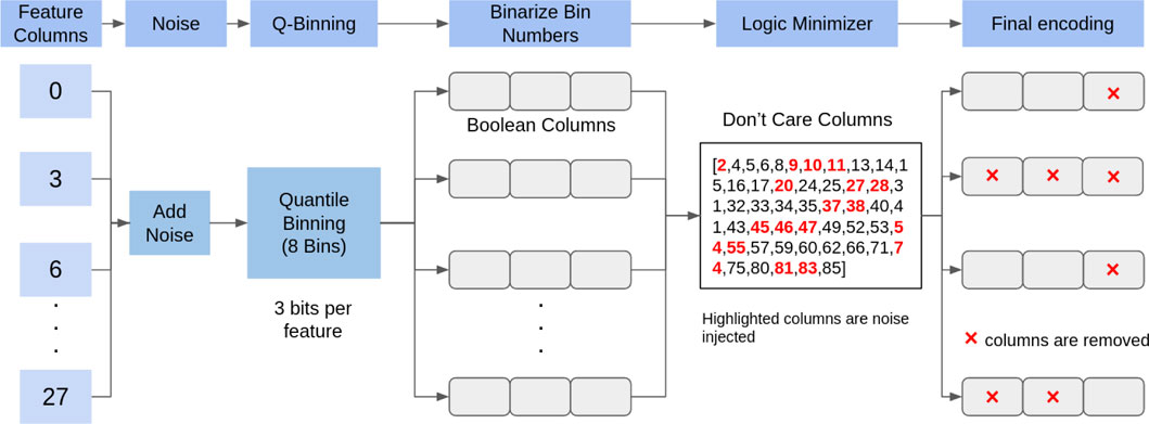
FIGURE 8. Breakdown of the preprocessing approach when using the Qbinning + Espresso workflow with respect to each feature column in the testing data.

These binary bins are then given to the Espresso algorithm to perform the minimization (in Figure 8, this corresponds to the logic minimizer block in the block diagram flow). The output of the algorithm is the rule set for these features.

We can therefore remove all the feature columns that are not within these rules as seen by the “Don’t Care Columns” block in Figure 8. These columns are not used by the minimizer to create the rules that link the Boolean data to the output class. We removed all the columns that deemed “Don’t Care Columns,” note in the final encoding block, shown with a red cross. It means that the entire column is no longer used by the TM. This highlights the redundancy removing capabilities of the logic minimizer, not only does it allow for feature extraction but it also acts as an effective noise filtering mechanism.

This forms a crucial indicator into why our encoding method performs better. Figure 8 shows that the highlighted red columns are the ones with noise injected into them; a large number of these columns have been indicated as redundant by the minimizer and are removed. Therefore, while the final encoding loses some valuable features resulting in reduced accuracy, the sensitivity of the TM remains high as much of the noise is filtered out, and there are still sufficient features remaining to form correct classifications.

Despite the noise injection at −15dB, the Breast Cancer data set still retains relatively high test accuracy at 75.6% (see Figure 1). To understand this behavior, we performed the principal component analysis of the testing data post noise injection, shown in Supplementary Figure S1. Through this we can understand how the covariance of the features is changed when some feature channels lose integrity; the plots show the first two PCA components of the raw data prior to Booleanization. It is clear that even at low SNRs benign data points are still very correlated, while the malignant data points are more scattered. We can see this in the higher specificity compared to sensitivity in Figure 1 as well. Only when the SNR is increased, both classes start to correlate together and therefore the classification problem becomes more defined and performance increases. Nevertheless, these results indicate the TM’s robustness to specific feature corruption if sufficient data points are gathered.

An important parameter of the Tsetlin machine is the number of clauses that are used per class. Increasing the number of clauses can be an effective method in increasing classification ability. More clauses result in a higher likelihood of clauses creating correct propositions that can describe the population. We explored this effect using the Breast Cancer data set, as shown in Figure 9. It is clear from the sensitivity results that increasing the number of clauses results in better performance at low SNRs. This suggests that even with the noise injected in specific feature columns it is still possible for the TM to generate good propositional logic when the number of opportunities to do so is increased (i.e., more clauses).

FIGURE 9

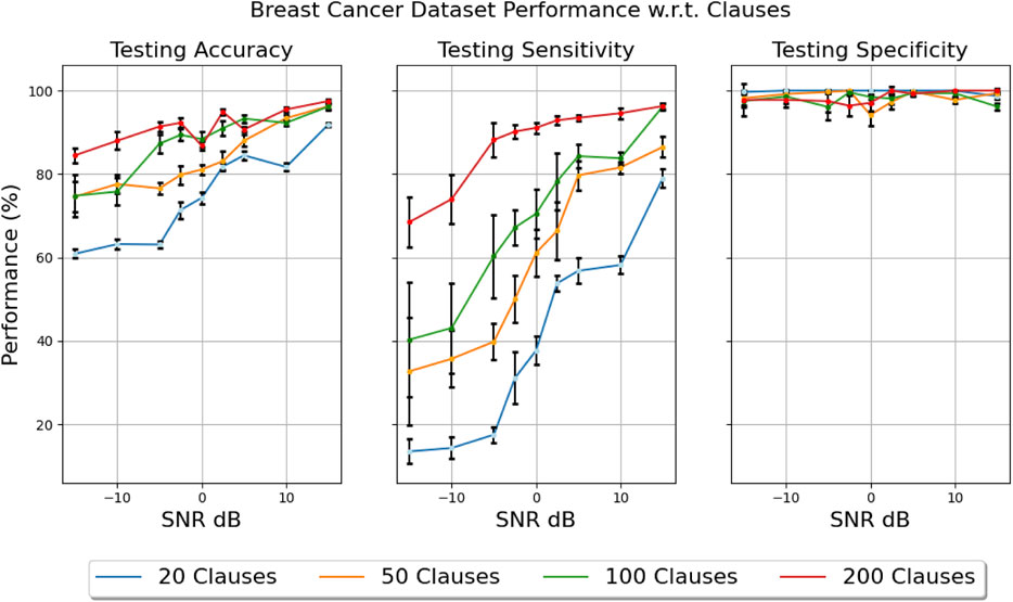
FIGURE 9. Effect on test accuracy when increasing clauses (using fixed threshold Booleanization). (Left) Testing accuracy for clauses ranging from 20 to 200. (Middle) Testing sensitivity for clauses ranging from 20 to 200. (Right) Testing specificity for clauses ranging from 20 to 200.

6 Impact of Noise Injection in Test Data

For this test, we trained the TM on clean data (i.e., without any noise added) and injected the testing data with noise across all the feature columns. Thus, we tested the universality of the training set with the following two hypotheses. First, if the training data is sufficiently diverse in the conditions it can describe each classification, and then it should be more robust to noise. Second, we tested if the rules generated by the minimizer and the resulting redundant features are still the same in the noisy testing population.

Figure 10 and Supplementary Figure S2 show the training vs. testing performance in terms of accuracy for the Breast Cancer and Parkinson’s data sets. We have summarized the preprocessing and TM configurations in Table 2. There are two behaviors that are present across both these results: first, the training accuracies remain high throughout (this is expected as the training data is clean); second, the Quantile binning + Espresso method performs better at low SNRs for both data sets, but as the SNR increases the fixed thresholding method appears to perform better.

FIGURE 10

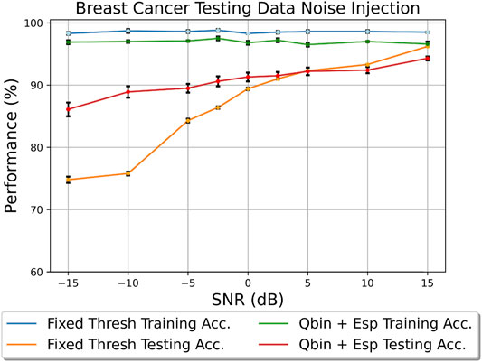
FIGURE 10. Breast Cancer 100 clauses testing data noise injection.

TABLE 2

TABLE 2. Comparing the Tsetlin machine and preprocessing configurations when injecting noise to all the test data on the Breast Cancer and Parkinson’s disease data sets.

Table 2 shows that having more features through fixed thresholding gives more advantages when the SNR increases. As seen through the PCA visualizations, the points for each class became more correlated, and having more bits for feature representation using fixed thresholding means greater granularity and therefore greater ability to capture patterns from the training set. At low SNR this is a disadvantage; the skewing of the data points between the training and testing due to increased noise injection means that patterns derived from the training set may not appear in the testing set. This is where the Quantile binning + Espresso is superior; through discretization, the slight variances due to noise injection can be minimized as the feature will most likely still be put into the same bin during quantile binning.To further prove the idea that discretization allows more robustness to noise, we conducted the same experiment on the Pima Indians Diabetes data set, as seen in Figure 11. We saw similar traits in the Breast Cancer and Parkinson’s disease data sets; the binning process allows for more robustness to noise. However, we also saw that at high SNR quantile binning performs better. This is due to the feature distributions of the data set. The age and glucose features are not normally distributed, and quantile binning is able to capture the data skew better than fixed thresholding. In Figure 11, we used six bins resulting in a 3-bit representation per feature. We chose six bins because this is the lowest discretization level before we start to see aliasing occurring in the data set leading to reduced performance. However, we also observed that having too many bins (more than 12) can result in empty bins in features where the distribution is close together. The choice of bin number should be attained through an initial trial and error exploration.

FIGURE 11

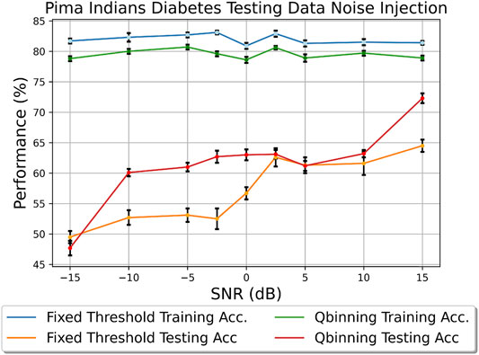
FIGURE 11. Testing data noise injection effect on the Pima Indians Diabetes data set.

Figure 12 examines the effect of changing the number of bins using quantile binning on the raw Pima Indians Diabetes data set. We can see that there is an optimal bin number at eight bins. Bins less than eight are not as effective in capturing enough information from the training data and bins above eight are gathering unnecessary information not seen in the testing data, hence the poorer performance of 10 bins at low SNRs.

FIGURE 12

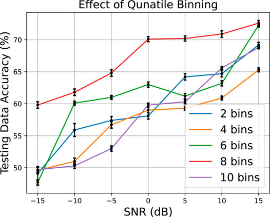
FIGURE 12. Effect of changing the number of bins using quantile binning.

As seen with the testing data selective injection, the Quantile binning + Espresso method offers better sensitivity across the SNR range, and this results in the better testing accuracy. Given the skew of more benign vs. malignant data points in the Breast Cancer data set, it is expected that the specificity should be high. In both cases for fixed threshold and quantile binning + Espresso, the specificity performance remains high echoing the results seen with selective testing column noise injection. To understand the testing accuracies more clearly, we examined the sensitivity and specificity’s for the Breast Cancer data set in Figure 13 across the SNR sweep. It is clear that the sensitivity for the quantile binning + Espresso is higher at low SNRs. We can see that having more granularity (using 10 bits per feature representation using fixed threshold) results in poorer performances at low SNRs.

FIGURE 13

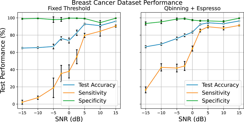
FIGURE 13. Testing data noise injection into the Breast Cancer data set.

More granular Boolean features result in a greater impact from the noise injection and therefore more difficult classification due to the increasing correlations between different features, as shown in Supplementary Figure S3. The SNR increases so does the covariance between features. Therefore, at higher SNR, the problem is better defined and hence higher sensitivity is expected. However, at low SNR, there is a larger correlation between the features leading to greater difficulty in forming a propositional logic that is more universal outside of the training data.

7 Impact of Noise Injection in Training Data

We injected noise across all the feature channels in the training data. This was performed to understand the robustness of the TM in terms of its classification boundaries when learning from noisy data. This is done by considering the TA states (the training parameters) after the training process; thus, we determined if each TA has reached an optimum position with respect to every other TA, that is, reached Nash equilibrium. In addition, we examined if our preprocessing methods can also aid in noise resilience.

To explore the effect on the training data using our noise-injection method, the PCA plots were used, as shown in Supplementary Figure S4. This figure highlights the difficulties present in this data set. Even at high SNR, we can see that there are many overlapping points. Nevertheless, the PCA plots follow the same relationship seen in the earlier plots when injecting testing data with noise; it can be seen that as the SNR increases the points corresponding to each class start to correlate more and therefore the problem becomes more defined for classification.

Figures 14, 15 show effects on the sensitivity and specificity of the training data when injected with noise using the two Booleanization methods. It can be seen that in both cases the specificity is consistently high across the SNR sweep for both Booleanization types, albeit for the quantile binning we saw a degradation in performance at the lower SNRs. The high specificity is explainable through the class imbalance in the data set. As seen through the PCA plots in Supplementary Figure S4, there are more benign points that correlate at higher SNRs.

FIGURE 14

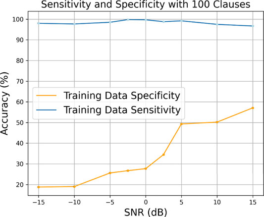
FIGURE 14. Sensitivity and specificity of the Pima Indians Diabetes data set using fixed thresholding when injecting the training data with noise.

FIGURE 15

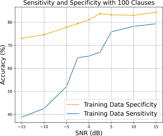
FIGURE 15. Sensitivity and specificity of the Pima Indians Diabetes data set using quantile binning when injecting the training data with noise.

We note that the sensitivity is much higher using quantile binning compared to that using fixed thresholding. This is most likely due to discretization masking the effects of the noise injection as seen with the results for Pima Indians Diabetes data set in the previous section. We know that there is still a large overlap between the two classes even at high SNR; therefore, they have more granularity and redundancy, which makes it harder for the TM to create all the appropriate logic propositions where we have 100 clauses per class. Therefore, having increased discretization means there are fewer features and fewer elements to be incorporated into the logic propositions, so it stands to reason that the sensitivity would be higher.

7.1 Nash Equilibrium Analysis

One of the fundamental tropes of noise resilience is mitigating the effects of epistemic uncertainty (Gal, 2016). In our experiment, we have defined this as the uncertainty of the clauses when creating a propositional logic. We have already seen that the clause computation is a simple logic operation between the include/exclude decisions of the TAs for each literal with the input literals (see Figure 1). In the TM, we know that each clause is aligned to a particular class; therefore, if we can group the clauses for each class, we can examine the decision boundaries of the TM.

We grouped each clause as a vector that contains the include/exclude decisions from its respective TAs. Then we were able to plot the clauses into a 2D space to determine if there are clear clusters for each class. Through this space we also gained insights into the TAs decisions with respect to every other TA at the clause level.

In order to translate our clause vectors to a 2D space, we used T-SNE (t-distributed stochastic neighbor embedding). We favored this method because unlike other dimensionality reduction techniques such as PCA, LDA, or K-means clustering, T-SNE is able to preserve more of the significance of the high-dimensional data structure in the low-dimensional map, whereas linear transformation methods focus more on pushing dissimilar points for apart (Van Der Maaten, 2014).

Through the clustering approach offered by T-SNE, we took a similar approach to Ficici et al. (2012) by examining the strategic view of agents (Clause vectors of TA decisions) in a cluster-based representation. We can use this to show that agents in the same cluster have the same pay-off and each cluster is aligned with a strategy. Therefore if the strategies are clear and explainable, we can conclude that we have reached Nash equilibrium.

For all the Nash equilibrium plots shown, the TM used 100 clauses per class and the number of used features can be seen in Figures 22, 23. Figures 16 and Supplementary Figure S5 show the T-SNE of clauses after training when using the fixed threshold preprocessing at both −15 and 15dB. To create these figures, we ran the TM noise–injected training pipeline 100 times and plotted the clause vectors from all these runs. In both SNR levels, it can be seen that there are clear boundaries present between the two clusters. Next, we examined the points to understand the strategy of each cluster. We saw that the positive clause of one class and the negative clause of the other are grouped together.

FIGURE 16

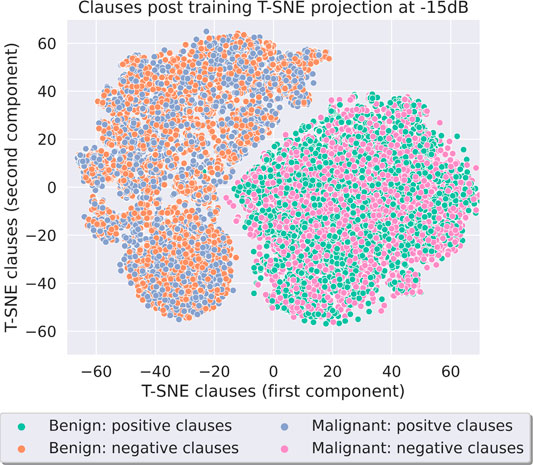
FIGURE 16. Breast Cancer clauses using fixed threshold at −15dB SNR.

This is expected at the TM clause level. We know that we have clauses aligned to each class, and we also know that half the clauses for each class will create propositional logic that supports the class and the other half will create logic that is against the class—this is referred to the polarity of the clause (either positive or negative). With this knowledge, we can say that our figures show that the TA states have reached Nash equilibrium. The clusters are formed of positive clause vectors for the class with TAs whose decisions are used to create propositional logic that supports that class, along with negative clause vectors from the other class whose TAs have been used to create propositional logic that supports the opposing class. The clusters are clear and the strategies they represent are explainable. Next, we determined if it is the preprocessing that allows for Nash equilibrium or whether it is the TM itself that is resilient to the noise impact. Therefore, we performed the same experiment using the quantile binning + Espresso preprocessing method, as seen in Figure 17 and Supplementary Figure S6. Once again the same characteristics are present at both the SNRs, and the same strategies are present in each of the clusters. Through Supplementary Figure S6, we also noted that the separation between the two main clusters is larger; therefore, the TA decisions that create the clause vectors are more similar as the noise is reduced.

FIGURE 17

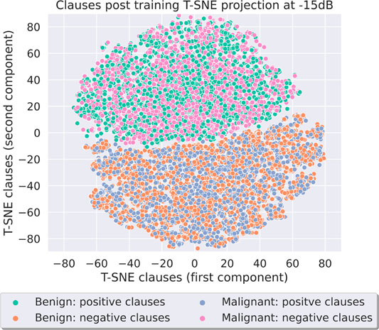
FIGURE 17. Breast Cancer using QBin + Esp at −15dB SNR.

Through Supplementary Figure S7 and Figure 18, it can be seen that the same characteristics that are present in the Breast Cancer data set are also seen here in the Parkinson’s disease data set. Once again, the distinctions between the two clusters are clear at both SNRs, and the strategies that each cluster represents matches the Breast Cancer T-SNE plots and what is expected from the TM algorithm in terms of clause polarity alignment. Once again, we performed the same experiment using the quantile binning + Espresso method on the Parkinson’s disease data set. Supplementary Figure S8 and Figure 19 show that the Nash equilibrium characteristics extend beyond both data set and the preprocessing method.

FIGURE 18

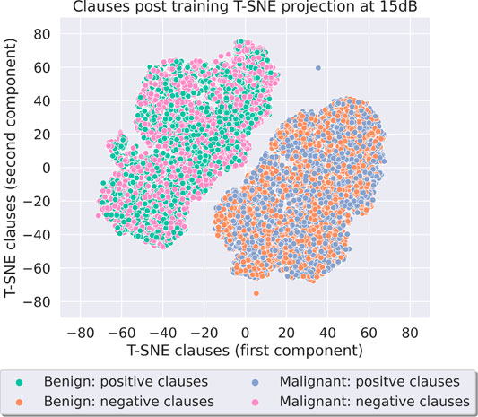
FIGURE 18. Parkinson’s disease using fixed thresholding at 15dB SNR.

FIGURE 19

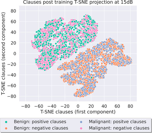
FIGURE 19. Parkinson’s disease using QBin + Esp at 15dB.

Figures 20, 21 shows that when the training data is injected with data, the Qbinning and Espresso method is not as effective as the fixed threshold method. Both encoding methods show an almost linear increase in sensitivity as the SNR is increased. This data set has fewer raw features compared to those of Breast Cancer and also more malignant data points compared to those of benign data points. The number of used features using fixed threshold are 220 for Parkinson’s and 300 for Breast Cancer, and the number of features used using the quantile binning + Espresso method are shown in Figures 22, 23.

FIGURE 20

FIGURE 20. Breast Cancer testing sensitivity of the two encoding procedures when the training data is injected with noise.

FIGURE 21

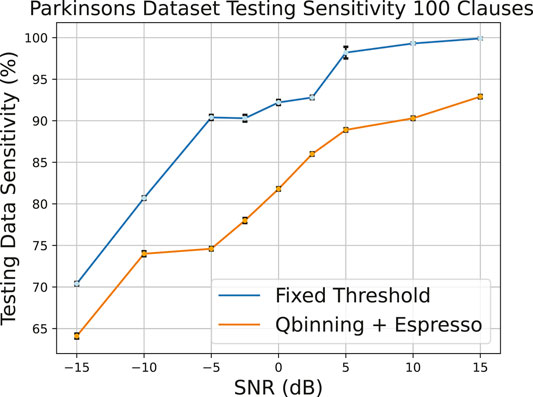
FIGURE 21. Parkinson’s disease testing sensitivity for the two encoding methods.

FIGURE 22

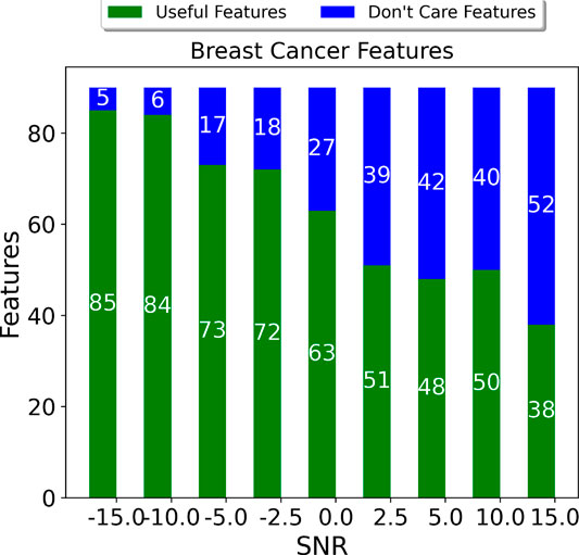
FIGURE 22. Espresso minimization ability for the Breast Cancer data set.

FIGURE 23

FIGURE 23. Espresso minimization ability for the Parkinson’s disease data set.

8 Logic Minimization and Comparative Analysis

This section explores the feature extraction capability of the logic minimizer as the SNR is increased from −15 to 15dB and the impact this Booleanized data has on both the TM and binary neural networks (BNNs) in terms of accuracy and estimated energy costs.

Figures 22, 23 show the effect of the Espresso minimizer when the SNR is increased from −15 to 15dB when the training data is injected across all columns. In both cases, we saw a linear increase in the number of “Don’t Care” features as the SNR increases. The increased noise at low SNR results in more skewed features, and it becomes more difficult to generate rules for these features and hence the smaller set of redundant features. Nevertheless, compared to the fixed threshold approach even at the lowest SNR for Breast Cancer for example, we have 84 features using our proposed approach compared to 300 features for fixed threshold.

The most comparable neural network architecture to the TM that can use the same preprocessing pipeline is the binary neural network (BNN). BNNs use binary activations, weights, and bit-wise XNOR for calculating the dot product (Geiger and Team, 2020).

In this section, we have compared the effects of noise on a BNN compared to that in the TM; we intend to show the effect of noise resilience through two different learning mechanisms: arithmetic weight–based learning vs. logic proposition–based learning.

We used the LARQ BNN software library to build a simple fully connected three layer BNN for all the experiments and compared with a TM that uses 100 clauses per class for all experiments (see Bannink et al. (2020) for further reading into this library).

Figure 24 shows the performance of a simple three layer BNN (300, 256, and 2) using the LARQ library vs. the TM with 100 clauses per class. We performed the fixed thresholding approach and trained both the ML models on noisy data as well as testing on equally noisy data on the Breast Cancer data set. Figure 24 shows that while the BNN offers better performance in the training accuracy when injected with noisy data, it is the TM that performs better in terms of testing accuracy. Through this we gained insights into the robustness of logic proposition–based learning. At low SNR, the TM testing accuracy is significantly higher meaning that the relationships formed through the propositional logic are more universal and less prone to overfitting compared to those in the BNN.

FIGURE 24

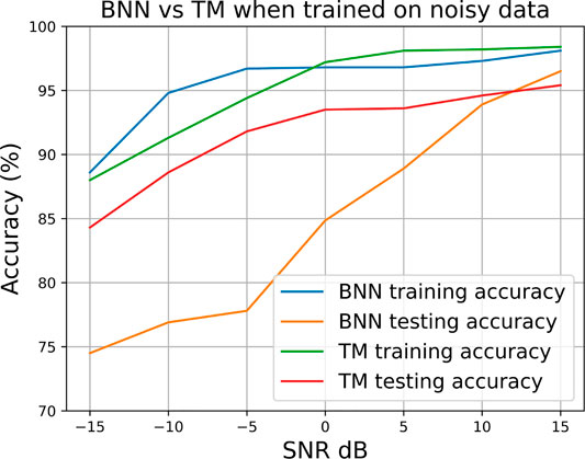
FIGURE 24. BNN vs. TM performance using fixed thresholding on the Breast Cancer data set.

We performed the same experiment using the proposed quantile binning + Espresso approach, as shown in Figure 25. Once again, a similar result with higher TM test accuracy compared to BNN test accuracy across the SNR sweep was observed. We also noted that BNN performs better when using the quantile binning + Espresso method; this further supports the arguments made from previous results that discretization at the right granularity can be a good measure for reducing the effects of noise and using a prior rule finding algorithm can also help in focusing the classifier toward only the most essential features.

FIGURE 25

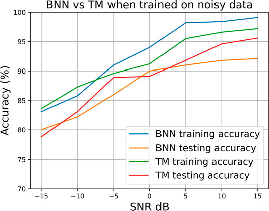
FIGURE 25. BNN vs. TM performance using QBin + Esp on the Breast Cancer data set.

For quantile binning + Espresso, the differences in performance are minor because the logic minimizer algorithm already found redundant features through rule mining in the normal disjunctive form—the same form in which the TM creates clause propositions. This added problem simplification helps the BNN.

One of the most important factors toward more efficient embedded implementations of ML applications is the number of training parameters; this will affect the overall memory footprint of the model (Geiger and Team, 2020). Table 3 shows the number of training parameters when injecting noise into the training data set using different preprocessing methods on both the TM and the BNN; we reported the number of training parameters at an SNR of −15 and 15dB.

TABLE 3

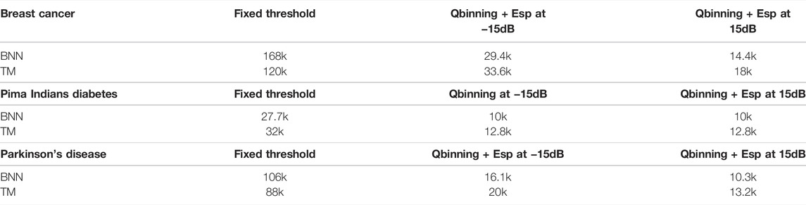
TABLE 3. Number of training parameters for the TM and BNN when injecting noise into training data for the three data sets.

We noted that both models have similar numbers of trainable parameters, but we have seen that the TM offers better resilience to noise. If memory constraints are paramount for a target platform, then we can start to reduce the number of clauses which will further reduce the number of training parameters at the cost of reduced performance, as seen in Figure 10.

When considering the performances of the quantile binning + Espresso, we have fewer features in the input layer of the BNN leading to similar memory footprint to the TM, but the performance of the BNN is poorer. To compensate this, a larger BNN with greater model complexity is required, but we chose to show the configuration closest to the TM complexity to highlight the performance vs. memory cost trade-off.

9 Estimated Energy Costs

To enable the transition to edge ML, it is vital to consider the energy cost associated with the training and inference. To calculate the energy, we extrapolated the energy per Boolean feature from the TM ASIC implementation presented in Wheeldon et al. (2020) and scaled these energy costs to the number of Boolean features in our two different approaches.

We have already seen that when the training data is injected with noise, the capability of the Espresso logic minimizer decreases with the SNR (Figures 22, 23). We applied the ASIC energy per data point measures to the number of features that are present post logic minimization for the Breast Cancer and Parkinson’s disease, shown in Figure 26. It can be seen clearly that as the SNR increases and the minimizer is able to deduce a more compact rule set, the number of features is reduced meaning fewer computations per clause and fewer state transition operations during the feedback stage.

FIGURE 26

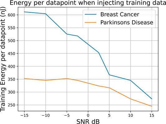
FIGURE 26. Energy per data point when injecting training data; more noise requires additional features for resilience and thereby affects the system energy.

When considering that the Breast Cancer training set has 300 data points for fixed threshold, we found that we used 25x less energy in training using the quantile binning + Espresso approach. It can bee seen that as the number of data points increased, we incurred far greater energy costs from fixed thresholding. Therefore, there is a trade-off to be made in balancing energy expenditure with achieving high sensitivity.

Nevertheless, we know that the feature spaces at the end of the quantile binning + Espresso are much smaller than that using fixed thresholding, as shown in Table 4. Here, we have compared the worst case feature sets for Breast Cancer, Pima Indians Diabetes, and Parkinson’s disease at −15dB with the respective features when using fixed thresholding.

TABLE 4

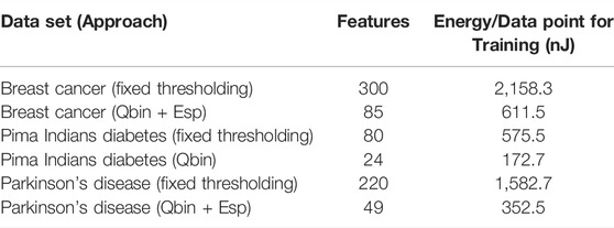
TABLE 4. Table showing the energy per data point for fixed thresholding vs. the proposed preprocessing approach. All models used 100 clauses per class.

10 Conclusion

By examining the impacts of noise injection into specific features, we showed how the removal of redundant features through a logic minimizer can be effective as a noise filtration method. We showed that discretization of the data using quantile binning can also be used as a method of masking the data corrupted by noise. By exploring the Nash equilibrium of the TM after training on noisy features, we showed that even through an SNR sweep on −15–15dB the TM is still able to generate distinct class boundaries where the strategies of the individual TAs are clear. We then examined how effective the TM is in comparison to BNNs; we showed that for both the preprocessing methods used in this study the TM test accuracy is better when the TM and BNN are trained on noisy data and that learning through creating logic proposition is a more robust way of dealing with noise corruption. We then provided insights into the effectiveness of TMs for edge ML implementation. The TM requires roughly the same number of parameters as BNNs, and through the energy per data point numbers we can see the effects of reducing the number of features on the energy expenditure.

Data Availability Statement

Publicly available data sets were analyzed in this study. This data can be found at: https://archive.ics.uci.edu/ml/datasets, https://archive.ics.uci.edu/ml/datasets/Breast+Cancer+Wisconsin+%28Diagnostic%29, https://www.kaggle.com/datasets/uciml/pima-indians-diabetes-database, https://archive.ics.uci.edu/ml/datasets/Parkinsons.

Author Contributions

TR is the lead scientist and author. He designed the experiments and evaluated the results and then generated the initial draft of the manuscript. RS is the principal investigator of the project. He formulated the problem including the use of Boolean minimization for feature engineering, wrote the manuscript with the lead author, and reviewed the scientific content. O-CG is one of the key investigators of the project. He co-designed the problem and led the use of Nash equilibrium to analyze convergence behavior under noise. AY is one of the key investigators of the project. He co-designed the problem and used energy costs for evaluating resilience under noise.

Conflict of Interest

The authors declare that the research was conducted in the absence of any commercial or financial relationships that could be construed as a potential conflict of interest.

Publisher’s Note

All claims expressed in this article are solely those of the authors and do not necessarily represent those of their affiliated organizations, or those of the publisher, the editors, and the reviewers. Any product that may be evaluated in this article, or claim that may be made by its manufacturer, is not guaranteed or endorsed by the publisher.

Supplementary Material

The Supplementary Material for this article can be found online at: https://www.frontiersin.org/articles/10.3389/fcteg.2021.778118/full#supplementary-material

Supplementary Figure S1 | First two principal components of Breast Cancer data set with noise injected to specific feature columns. The blue dots represent benign data points and the orange dots represent malignant data points. As the SNR is increased from (A) to (F) the points corresponding to each class become more correlated and the problem space becomes more defined.

Supplementary Figure S2 | Parkinson’s disease 100 clauses testing data noise injection.

Supplementary Figure S3 | PCA eigenvalues of the Breast Cancer data set across the SNR sweep.

Supplementary Figure S4 | First and second principal components of the Pima Indians Diabetes data set when the training data is injected with noise. The blue dots represent benign data points and the orange dots represent malignant data points. As the SNR is increased from (A) to (F) the points corresponding to each class start to correlate more and the classification problem becomes more defined.

Supplementary Figure S5 | Breast Cancer clauses using fixed threshold at 15dB SNR.

Supplementary Figure S6 | Breast Cancer using QBin + Esp at 15dB SNR.

Supplementary Figure S7 | Parkinson’s disease using fixed threshold at −15dB SNR.

Supplementary Figure S8 | Parkinson’s disease using QBin + Esp at −15dB.

References

Abeyrathna, K. D., Granmo, O.-C., Shafik, R., Yakovlev, A., Wheeldon, A., Lei, J., et al. (2020). “A Novel Multi-step Finite-State Automaton for Arbitrarily Deterministic Tsetlin Machine Learning,” in International Conference on Innovative Techniques and Applications of Artificial Intelligence (Springer), 108–122. doi:10.1007/978-3-030-63799-6_8

CrossRef Full Text | Google Scholar

Alaoui, E. A. A., Tekouabou, S. C. K., Hartini, S., Rustam, Z., Silkan, H., and Agoujil, S. (2021). Improvement in Automated Diagnosis of Soft Tissues Tumors Using Machine Learning. Big Data Min. Anal. 4, 33–46. doi:10.26599/bdma.2020.9020023

CrossRef Full Text | Google Scholar

Alizadehsani, R., Roshanzamir, M., Hussain, S., Khosravi, A., Koohestani, A., Zangooei, M. H., et al. (2021). Handling of Uncertainty in Medical Data Using Machine Learning and Probability Theory Techniques: a Review of 30 Years (1991-2020). Ann. Oper. Res. 12, 14. doi:10.1007/s10479-021-04006-2

CrossRef Full Text | Google Scholar

Amrane, M., Oukid, S., Gagaoua, I., and Ensari, T. (2018). “Breast Cancer Classification Using Machine Learning,” in 2018 Electric Electronics, Computer Science (Istanbul, Turkey: Biomedical Engineerings’ Meeting), 1–4. doi:10.1109/EBBT.2018.8391453

CrossRef Full Text | Google Scholar

Bailey, S. (2012). Principal Component Analysis with Noisy And/or Missing Data, 124. Chicago: University of Chicago Press, 1015–1023. doi:10.1086/668105Principal Component Analysis with Noisy And/or Missing DataPublications Astronomical Soc. Pac.

CrossRef Full Text | Google Scholar

Baldi, P. (2018). Deep Learning in Biomedical Data Science. Annu. Rev. Biomed. Data Sci. 1, 181–205. doi:10.1146/annurev-biodatasci-080917-013343

CrossRef Full Text | Google Scholar

Bannink, T., Bakhtiari, A., Hillier, A., Geiger, L., de Bruin, T., Overweel, L., et al. (2020). Larq Compute Engine: Design, Benchmark, and Deploy State-Of-The-Art Binarized Neural Networks. CoRR abs/2011.

Google Scholar

Brayton, R. K., Sangiovanni-Vincentelli, A. L., McMullen, C. T., and Hachtel, G. D. (1984). Logic Minimization Algorithms for VLSI Synthesis. USA: Kluwer Academic Publishers.

Google Scholar

Cao, Z., Yang, G., Chen, Q., Chen, X., and Lv, F. (2020). Breast Tumor Classification through Learning from Noisy Labeled Ultrasound Images. Med. Phys. 47, 1048–1057. doi:10.1002/mp.13966

PubMed Abstract | CrossRef Full Text | Google Scholar

Castiglioni, I., Rundo, L., Codari, M., Di Leo, G., Salvatore, C., Interlenghi, M., et al. (2021). Ai Applications to Medical Images: From Machine Learning to Deep Learning. Physica Med. 83, 9–24. doi:10.1016/j.ejmp.2021.02.006

CrossRef Full Text | Google Scholar

Driggs, D., Selby, I., Roberts, M., Gkrania-Klotsas, E., Rudd, J. H. F., Yang, G., et al. (2021). Machine Learning for Covid-19 Diagnosis and Prognostication: Lessons for Amplifying the Signal while Reducing the Noise. Radiol. Artif. Intelligence 3, e210011. doi:10.1148/ryai.2021210011

CrossRef Full Text | Google Scholar

Ficici, S. G., Parkes, D. C., and Pfeffer, A. (2012). Learning and Solving many-player Games through a Cluster-Based Representation, 3253. CoRR abs/1206.

Google Scholar

Gal, Y. (2016). Uncertainty in Deep Learning. [Ph.D. thesis]. Cambridge: University of Cambridge. Available at: https://mlg.eng.cam.ac.uk/yarin/thesis/thesis.pdf

Google Scholar

Galivanche, R., and Reddy, S. M. (1987). “A Parallel Pla Minimization Program,” in 24th ACM/IEEE Design Automation Conference (IEEE)–607. doi:10.1145/37888.37983

CrossRef Full Text | Google Scholar

Geiger, L., and Team, P. (2020). Larq: An Open-Source Library for Training Binarized Neural Networks. Joss 5, 1746. doi:10.21105/joss.01746

CrossRef Full Text | Google Scholar

Granmo, O. C. (2021). The Tsetlin Machine – a Game Theoretic Bandit Driven Approach to Optimal Pattern Recognition with Propositional Logic. arXiv.

Google Scholar

Granmo, O., Glimsdal, S., Jiao, L., Goodwin, M., Omlin, C. W., and Berge, G. T. (2019). The Convolutional Tsetlin Machine, 09688. CoRR abs/1905.

Google Scholar

Gupta, S., and Gupta, A. (2019). Dealing with Noise Problem in Machine Learning Data-Sets: A Systematic Review. Proced. Comp. Sci. 161, 466–474. The Fifth Information Systems International Conference, 23-24 July 2019, Surabaya, Indonesia. doi:10.1016/j.procs.2019.11.146

CrossRef Full Text | Google Scholar

Han, B., Yao, Q., Yu, X., Niu, G., Xu, M., Hu, W., et al. (2018). Co-sampling: Training Robust Networks for Extremely Noisy Supervision, 06872. CoRR abs/1804.

Google Scholar

Jiao, L., Zhang, X., Granmo, O.-C., and Abeyrathna, K. D. (2021). On the Convergence of Tsetlin Machines for the Xor Operator. arXiv.

Google Scholar

Lei, J., Rahman, T., Shafik, R., Wheeldon, A., Yakovlev, A., Granmo, O.-C., et al. (2021). Low-power Audio Keyword Spotting Using Tsetlin Machines. Jlpea 11, 18. doi:10.3390/jlpea11020018

CrossRef Full Text | Google Scholar

Lei, J., Wheeldon, A., Shafik, R., Yakovlev, A., and Granmo, O.-C. (2020). From Arithmetic to Logic Based AI: A Comparative Analysis of Neural Networks and Tsetlin Machine. Proc. IEEE ICECS., 1–4. doi:10.1109/icecs49266.2020.9294877

CrossRef Full Text | Google Scholar

McCluskey, E. J. (1956). Minimization of Boolean Functions*. Bell Syst. Tech. J. 35, 1417–1444. doi:10.1002/j.1538-7305.1956.tb03835.x

CrossRef Full Text | Google Scholar

Obermeyer, Z., and Emanuel, E. J. (2016). Predicting the Future - Big Data, Machine Learning, and Clinical Medicine. N. Engl. J. Med. 375, 1216–1219. doi:10.1056/NEJMp1606181

PubMed Abstract | CrossRef Full Text | Google Scholar

Pechenizkiy, M., Tsymbal, A., Puuronen, S., and Pechenizkiy, O. (2006). “Class Noise and Supervised Learning in Medical Domains: The Effect of Feature Extraction,” in 19th IEEE Symposium on Computer-Based Medical Systems (New York: IEEE), 708–713. doi:10.1109/CBMS.2006.65

CrossRef Full Text | Google Scholar

Quine, W. V. (1952). The Problem of Simplifying Truth Functions. The Am. Math. Monthly 59, 521–531. doi:10.1080/00029890.1952.11988183

CrossRef Full Text | Google Scholar

Romero, I. (2010). PCA-based Noise Reduction in Ambulatory ECGs. Comput. Cardiol., 677–680.

Google Scholar

Sabzevari, M., Martínez-Muñoz, G., and Suárez, A. (2018). Vote-boosting Ensembles. Pattern Recognition 83, 119–133. doi:10.1016/j.patcog.2018.05.022

CrossRef Full Text | Google Scholar

Schooltink, W. (2020). Testing the Sensitivity of Machine Learning Classifiers to Attribute Noise in Training Data.

Google Scholar

Schulz, L. O., Bennett, P. H., Ravussin, E., Kidd, J. R., Kidd, K. K., Esparza, J., et al. (2006). Effects of Traditional and Western Environments on Prevalence of Type 2 Diabetes in pima Indians in mexico and the u.S. Diabetes Care 29, 1866–1871. doi:10.2337/dc06-0138

PubMed Abstract | CrossRef Full Text | Google Scholar

Shafik, R., Wheeldon, A., and Yakovlev, A. (2020). “Explainability and Dependability Analysis of Learning Automata Based Ai Hardware,” in 2020 IEEE 26th International Symposium on On-Line Testing and Robust System Design (New York: IEEE), 1–4. doi:10.1109/IOLTS50870.2020.9159725

CrossRef Full Text | Google Scholar

Shanab, A. A., Khoshgoftaar, T. M., Wald, R., and Napolitano, A. (2012). “Impact of Noise and Data Sampling on Stability of Feature Ranking Techniques for Biological Datasets,” in 2012 IEEE 13th International Conference on Information Reuse Integration, 415–422. doi:10.1109/IRI.2012.6303039

CrossRef Full Text | Google Scholar

Shanthini, A., Vinodhini, G., Chandrasekaran, R. M., and Supraja, P. (2019). A Taxonomy on Impact of Label Noise and Feature Noise Using Machine Learning Techniques. Soft Comput. 23, 8597–8607. doi:10.1007/s00500-019-03968-7

CrossRef Full Text | Google Scholar

Sukhbaatar, S., and Fergus, R. (2014). Learning from Noisy Labels with Deep Neural Networks. arXiv preprint arXiv:1406.2080 2, 4.

Google Scholar

Thottakkara, P., Ozrazgat-Baslanti, T., Hupf, B. B., Rashidi, P., Pardalos, P., Momcilovic, P., et al. (2016). Application of Machine Learning Techniques to High-Dimensional Clinical Data to Forecast Postoperative Complications. PLOS ONE 11, e0155705–19. doi:10.1371/journal.pone.0155705

PubMed Abstract | CrossRef Full Text | Google Scholar

Tice, A. M., and Farag, H. A. (2019). Machine Learning in Microbiology: Finding the Signal in the Noise. Clin. Microbiol. Newsl. 41, 121–127. doi:10.1016/j.clinmicnews.2019.06.004

CrossRef Full Text | Google Scholar

Van Der Maaten, L. (2014). Accelerating T-Sne Using Tree-Based Algorithms. J. Machine Learn. Res. 15, 3221–3245.

Google Scholar

Wheeldon, A., Shafik, R., Rahman, T., Lei, J., Yakovlev, A., and Granmo, O.-C. (2020). Learning Automata Based AI Hardware Design for IoT. Phil. Trans. A R. Soc.

Google Scholar

Wheeldon, A., Yakovlev, A., Shafik, R., and Morris, J. (2021). “Low-latency Asynchronous Logic Design for Inference at the Edge,” in 2021 Design, Automation Test in Europe Conference Exhibition (DATE), 370–373. doi:10.23919/DATE51398.2021.9474126

CrossRef Full Text | Google Scholar

Wolberg, W. H., and Mangasarian, O. L. (1990). Multisurface Method of Pattern Separation for Medical Diagnosis Applied to Breast Cytology. Proc. Natl. Acad. Sci. U.S.A. 87, 9193–9196. doi:10.1073/PNAS.87.23.9193

PubMed Abstract | CrossRef Full Text | Google Scholar