PID control: Resilience with respect to controller implementation

1 Introduction

The proportional–integral–derivative (PID) controller was first proposed in 1922 by Minorsky (1922) and first applied in industrial applications in 1939 (Bennett, 1993). Since then, it has been considered an effective tool and is one of the most common control schemes that have dominated the majority of industrial processes and mechanical systems because of its versatility, high reliability, and ease of operation (Astrom and Hagglund, 2006). PID controllers can be manually tuned appropriately by the operators and control engineers based on the empirical knowledge when the mathematical model of the controlled plant is unknown. Some classical tuning methods, such as Ziegler–Nichols method (Ziegler and Nichols, 1942), Chien–Hrones–Reswick method (Chien et al., 1952), IMC (Rivera et al., 1986), S-IMC (Skogestad, 2003), robust IMC (Vilanova, 2008), and MoReRT (Alfaro and Vilanova, 2016), are applied to the process control, and the performance is then significantly outperformed compared to the one that is manually tuned.

One of the major drawbacks of the basic parallel formulations of PID controllers is the effects of proportional and derivative kick. The changes in the set point cause an impulse signal or sudden change in the controller output as well as in the output response (Johnson, 2005). The controller output is given to the final control elements like control valve, motor, or electronic circuit in which the spikes create serious problems. In order to minimize these effects, modified forms of parallel controller structures such as ID-P and I-PD are usually considered in practice as suggested by Ogawa and Kano (2008) and Ang et al. (2005).

Another motivation for the appropriate selection of the controller structure comes from the differences that arise depending on the mode of operation of the designed closed-loop. This is a common factor (O’Dwyer, 2009) that all approaches face: the frequently referred topic of set-point tracking vs. disturbance rejection performance. It is well-known (Alcantara et al., 2013) that there is an inherent tradeoff between both modes of operation in addition to the also well-known performance/robustness tradeoff. This distinction has made available in recent years a number of research works that analyze and provide tuning solutions to each one of the operational modes under a variety of performance indexes as well as control constraints. However, it has also been recognized (Shinskey, 2002; Vilanova et al., 2017) that disturbance rejection is much more important than set-point tracking for many process control applications, leading set-point tracking to a secondary level of interest. Therefore, a controller design that emphasizes disturbance rejection rather than set-point tracking is an important design problem that, even if it has been the focus of research, it may have not received the appropriate attention. One way of focusing explicitly on load disturbance is by the appropriate selection of the controller equation. In the ideal PID formulation, all the three modes process the error signal and therefore both the reference and the disturbance signals. However, industrial software packages (Ang et al., 2005) used to offer a choice menu where different implementations are available. One can choose which controller modes are fed with the reference signal. From this aspect, we can go, for example, from PID to PI-D, where the derivative term just acts on the process output, or the I-PD where the error signal is just seen by the integral term.

On the basis of the previous situation, the authors aim to focus on the idea of resilience of PID tuning rules. This is the idea of tuning rules that guarantee appropriate performance and robustness even when applied on a different PID formulation from the one the tuning rule was conceived for. We do not refer in this work to the problem of not appropriately converting the tuning equations and making them consistent with the controller formulation. This has already been addressed by Alfaro and Vilanova (2012a) for what matters to the changes in the PID equation. However, a deep analysis of the implications that the signal processed by each controller mode does have on the resulting closed-loop control performance is still needed. This will serve as a basis for evaluating the resilience of the tuning.

Vilanova et al. (2018a) presented a robust tuning rule for I-PD controllers from the point of view of solving the servo vs. regulation choice for tuning. From this perspective, the I-PD implementation is conceived as an alternative that provides a structural solution to tradeoff tuning. The proposal states that a direct, simple, and efficient solution is found if the controller tuning is addressed for the servo mode but using the I-PD controller structure. The effects of the usual tuning rules implemented as an I-PD controller are analyzed, and the loss of performance of the usual IMC tuning, for example, is reported. However, it is to be noted that the IMC tuning is essentially a servo tuning. Therefore, when implemented as an I-PD controller, the loss of performance is expected because the proportional term does not process the process output. This analysis, however, even if correct, is not general and does not imply that all tunings will underperform when implemented as an I-PD controller. In other words, the lack of resilience should not be taken for granted.

On the basis of the previous scenario, the purpose of this work is to gain insights into such a resilience concept. We analyze the performance and robustness of the implementation of simple robust tuning (SRT) presented by Alfaro and Vilanova (2013) when I-PD and PID formulations are considered both a 1-DoF and a 2-DoF controller. The evaluation is confronted with robust tuning explicitly designed for the I-PD controller as presented by Vilanova et al. (2018a). This comparison is not conducted with the aim of establishing the best tuning but to illustrate the advantages of the resilience with respect to controller implementation.

The following section reviews the concepts of fragility and resilience with respect to robustness and performance as they will be used in the work. Next, the control problem formulation is presented, and the differences between PID controller implementations are stated. Notation is introduced regarding PID implementation in terms of signal processing. Following this, simple robust tuning (SRT) is presented. Section 5 presents an evaluation of a benchmark process and different robustness levels, followed by a discussion on the resilience idea and some concluding remarks.

2 Fragility evaluation

Alfaro (2007) presented the concept of controller fragility. Fragility introduces a measure of the change (in fact, the loss) in the controlled closed-loop system robustness due to a change in the controller parameters (changes up to 20% are usually associated to the final fine-tuning of the controller). The loss of robustness caused because of this change in the controller parameters is evaluated by means of the delta 20 fragility index. Values of this index determine if the tuning is fragile (>0.5), non-fragile (≥0.5), or resilient (≥0.1).

Two main differences arise in the idea presented here. First of all, the property that may change is not robustness but the performance. Second, the motivation for such a change is not a change in the controller parameters but a change in the equation that implements the controller.

The notion we introduce in this work refers to controller implementation. In fact, the main difference with respect to the notion of the controller’s fragility presented by Alfaro (2007) is the effect generated by an eventual small change on the controller parameters, whereas here the tuning remains fixed, but the controller equations are the ones that may change. The changes in the controller equation that are considered here mainly refer to reference processing. Even one of the degrees of freedom may be lost. What matters here is which controller modes (proportional and/or integral) process the reference signal and in which way (using the set-point weight—2-DoF—or not—1-DoF)¹. In all such cases, the feedback properties remain unchanged. Therefore, the control system will experience a potential reduction in the tracking performance. Its robustness and regulation properties will remain unchanged.

The classification proposed by Alfaro (2007) as fragile, non-fragile, or resilient, in terms of the delta 20 fragility index, is chosen because the change in the controller parameters may turn a control system with a highly robust controller (with M_s between 1.2 and 1.4) into one with minimum acceptable robustness (M_s ≈ 2.0)².

In this case, it is not possible to get an idea of relative loss because the change in the controller is structural. It gets difficult to establish a single number as a threshold where we can say whether the performance loss is acceptable or not. This will be process- and application-dependent. In addition, it must be considered that as the effects of the implementation will be just on tracking, the evaluation will depend on the measure that the control system will operate as a regulator or as a servo. There are too many considerations that prevent a single, objective definition to be established. However, even in this different framework, it is the author’s opinion to better consider a conceptual extension of the initial fragility index along the same lines as presented by Alfaro and Vilanova (2012b) for the idea of performance fragility with respect to a small variation in the controller parameters.

Therefore, we propose to extend the same classification of performance-fragile, non-fragile, and resilient controllers as presented by Alfaro and Vilanova (2012b), but with respect to a change in the controller implementation rather than a 20% change in its parameters. Of course, this adoption is made with the idea of avoiding to introduce other different and subjective measures. Considering a change in the controller’s equation implementation, the delta performance-fragility index, PFI_Δ, could define the maximum loss of the control system performance with respect to the original equation the controller was conceived for (Alfaro and Vilanova, 2012b):

$PF{I}_{\mathrm{\Delta }}\doteq \frac{J_{e\mathrm{\Delta }}^m}{J_e^o}-1,(1)$

where $J_e^o$ is the performance measure index evaluated on the nominal system and $J_{e\mathrm{\Delta }}^m$ is the extreme value for the same index evaluated when a Δ variation in the controller parameters is introduced. This index usually takes the form of an integral criterion such as IAE, ITAE, ISE, and ITSE. However, it does not need to be constrained to this form. Based on the PFI_Δ, the controller’s performance, its fragility degree is defined as follows:

• Performance-fragile PID controller: A PID controller is performance-fragile if its delta performance fragility index is higher than 0.50, PFI_Δ > 0.50.

• Performance-non-fragile PID controller: A PID controller is performance-non-fragile if its delta performance fragility index is less than or equal to 0.50, PFI_Δ ≤ 0.50.

• Performance-resilient PID controller: A PID controller is performance-resilient if its delta performance fragility index is less than or equal to 0.10, PFI_Δ ≤ 0.10.

3 Control problem and PID controller formulation

In this section, we revise the control problem formulation as well as the formulation of the PID controller equation and the different options for error, feedback, and reference signal processing. As some of the concepts, especially what matters to the control problem are well-known, the presentation will be succinct.

3.1 Control problem

Consider a closed-loop control system, as shown in Figure 1, where P(s) is the controlled process model and C_r(s) and C_y(s) are the transfer functions of the set-point controller and the feedback controller, respectively. In this system, r(s) is the set point, u(s) is the controller output signal, d(s) is the load disturbance, and y(s) is the controlled process variable.

FIGURE 1

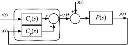
FIGURE 1. Closed-loop control system.

The control system output is

$y\left(s\right)=M_{yr}\left(s\right)r\left(s\right)+M_{yd}\left(s\right)d\left(s\right),(2)$

where the servo-control and the regulatory control closed-loop transfer functions are

$M_{yr}\left(s\right)=\frac{C_r\left(s\right)P\left(s\right)}{1+C_y\left(s\right)P\left(s\right)}(3)$

and

$M_{yd}\left(s\right)=\frac{P\left(s\right)}{1+C_y\left(s\right)P\left(s\right)},(4)$

respectively, that are related by

$M_{yr}\left(s\right)=C_r\left(s\right)M_{yd}\left(s\right).(5)$

As the control system closed-loop characteristic polynomial is

$p\left(s\right)=1+C_y\left(s\right)P\left(s\right),(6)$

the control system relative stability depends on the controlled process model and the feedback controller parameters but not on the set-point controller parameters that are not included in the feedback controller transfer function.

Given a controlled process model P(s) and the controller C(s) = {C_r(s), C_y(s)}, control algorithm parameters must be selected considering the control system robustness—relative stability—and its performance under a selected design metric.

3.2 PID controllers

As a general controller, the two-degree-of-freedom (2-DoF) proportional integral derivative control algorithm,

$u\left(t\right)=K_p\left\{\beta r\left(t\right)-y\left(t\right)+\frac{1}{T_i}{\int }_0^t\left[r\left(\xi \right)-y\left(\xi \right)\right]\mathrm{d}\xi +T_d\frac{\mathrm{d}\left[\gamma r\left(t\right)-y\left(t\right)\right]}{\mathrm{d}t}\right\},(7)$

is considered that can be expressed in the s domain as

$u\left(s\right)=K_p\left\{\beta r\left(s\right)-y\left(s\right)+\frac{1}{T_{i}s}\left[r\left(s\right)-y\left(s\right)\right]+\frac{T_{d}s}{\alpha T_{d}s+1}\left[\gamma r\left(s\right)-y\left(s\right)\right]\right\},(8)$

where K_p is the controller proportional gain, T_i is the integral time, T_d is the derivative time, α is the derivative filter constant, β is the proportional set-point weight factor, and γ is the derivative set-point weight factor. It is to be noted that in Eq. 8, as usual practice, a first-order filter has been added to the derivative term.

Controller output Eq. 8 can be expressed as

$u\left(s\right)=C_r\left(s\right)r\left(s\right)-C_y\left(s\right)y\left(s\right),(9)$

and the control system error signal is

$e\left(s\right)=r\left(s\right)-y\left(s\right).(10)$

Selection of the set-point weight factors ß and γ allows to obtain the different members of the PID controller “family”: the general 2-DoF PID controller PID_e2—control modes act on different weighted error signals; the 2-DoF PID controller PI_eD_y2—derivative mode acts only on the feedback signal; the basic one-degree-of-freedom (1-DoF) PID controller PID_e1—all control modes act on the error signal; the 1-DoF PI_eD_y1 controller—proportional and integral control modes act on the error; and the 1-DoF I_ePI_y1 controller—only the integral control acts on the error signal, as listed in Table 1. Figure 2 shows a generic block diagram of a 2-DoF PID controller, showing the role of the ß and γ weights according to this table.

TABLE 1

TABLE 1. PID controller “family.”

FIGURE 2

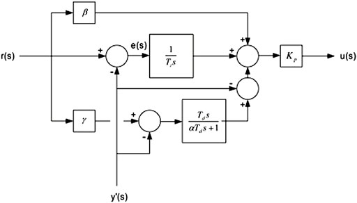
FIGURE 2. Block diagram of a PID controller Eq. 8 representing all situations for the PID controller’s “family” shown in Table 1.

From Eq. 8 and Table 1, it is found that all the aforementioned PID control algorithms provide the same feedback controller but different regulatory controllers as follows—considering here only controllers with no derivative “kick” (γ = 0):

• Feedback controller of all the PID algorithms:

$C_y\left(s\right)=K_p\left(1+\frac{1}{T_{i}s}+\frac{T_{d}s}{\alpha T_{d}s+1}\right).(11)$

• Set-point controller of the PI_eD_y2:

$C_r\left(s\right)=K_p\left(\beta +\frac{1}{T_{i}s}\right).(12)$

• Set-point controller of the PI_eD_y1:

$C_r\left(s\right)=K_p\left(1+\frac{1}{T_{i}s}\right).(13)$

• Set-point controller of the I_ePD_y1:

$C_r\left(s\right)=\frac{K_p}{T_{i}s}.(14)$

In the I-PD controller structure, all three parameters contribute to the disturbance attenuation as all three parameters process the output signal. On the other hand, only the integral time constant contributes to the tracking performance. Therefore, the final allocation of the controller gains should result in different controller tunings depending on the use of an I-PD or a PID. Questions such as the following ones naturally arise: will the performance of the I-PD degrade significantly from the PID one? Will it be beneficial to elaborate tuning rules specifically for the I-PD configuration?

4 Simple robust tuning

As presented, the simple robust tuning (SRT) method by Alfaro and Vilanova (2013) is considered for evaluation with respect to the different PID controller implementations. In this section, the SRT formulation, tuning equations, and robustness characterization are presented. The SRT equations for the 2-DoF PID controllers (PI_eD_y2) are obtained on the basis of a performance/robustness tradeoff analysis.

The SRT method regards a controlled process as a generic SOPDT model, given by the following transfer function:

$\begin{array}{ll}\hfill P\left(s\right)& =\frac{K{\mathrm{e}}^{-Ls}}{\left(Ts+1\right)\left(aTs+1\right)},\hfill \\ \hfill & 0\le a\le 1,0.1\le {\tau }_L=\frac{L}{T}\le 2,\hfill \end{array}(15)$

covering first- and second-order plus dead-time overdamped processes.

The control system performance is optimized under the integrated absolute error (IAE) cost functional

$J_e\doteq {\int }_0^{\infty }|e\left(t\right)|\mathrm{d}t={\int }_0^{\infty }|r\left(t\right)-y\left(t\right)|\mathrm{d}t,(16)$

and its robustness is measured with the maximum sensitivity

$M_S\doteq \underset{\omega }{\max }|S\left(\mathrm{j}\omega \right)|=\underset{\omega }{\max }\frac{1}{|1+C_y\left(\mathrm{j}\omega \right)P\left(\mathrm{j}\omega \right)|}.(17)$

As additional performance evaluation metrics, the control effort total variation

$T{V}_u\doteq \sum _{k=1}^{\infty }|u_{k+1}-u_k|,(18)$

and the controller output instant change to a set-point step change

$\mathrm{\Delta }{u}_0\doteq \beta K_p\mathrm{\Delta }r,(19)$

can be used.

Analysis of the regulatory control performance and robustness shows that for a model with a given time constant ratio a, increasing the control system target robustness $M_S^t$ results in a substantial reduction in the controller gain K_p but has a negligible effect on the controller integral time T_i and the derivative time T_d. As a result, tuning equations that are independent of the desired robustness are obtained for the T_i and T_d controller parameters. On the other hand, K_p is used to match the control system target robustness level and becomes the only robustness-dependent controller parameter. As the controller gain depends on the control system robustness, the proportional set-point weight factor ß depends on it as well.

The SRT equations are of the general form³:

$K_p=\mathbf{H}\left(T,{\tau }_L,a;M_S^t\right),(20)$

$T_i=\mathbf{F}\left(T,{\tau }_L,a\right),(21)$

$T_d=\mathbf{G}\left(T,{\tau }_L,a\right),(22)$

$\beta =\mathbf{Q}\left({\tau }_L;M_S^t\right).(23)$

SRT equations H, F, G, and Q for four target robustness levels, $M_S^t\in$ {minimum (2.0), low (1.8), intermediate (1.6), high (1.4)}, and controlled process models with five time constant ratios, a ∈ {fopdt (0.0), sopdt (0.25, 0.50, 0.75), dppdt (1.0)}, can be found in Alfaro and Vilanova (2013).

5 Performance evaluation

Having presented the SRT tuning equations, now it is time to evaluate their performance regarding the operation of the closed-loop control system with the PID controller implemented under different variations, say PI_eD_y2, PI_eDy1, and I_ePD_y1. Performance is evaluated with respect to regulatory control and servo-control operation. Also, robustness of the control system should be taken into account. The evaluation will be conducted by considering a usual benchmark process model from Åström and Hägglund (2000) and also considering the robust I-PD tuning from Vilanova et al. (2018a) to have a reference of robust tuning regarding I_ePD_y1 implementation.

The evaluation is conducted using the following steps: first of all, the process models are obtained, and the corresponding controllers are adjusted according to the presented SRT tuning rule. Next, the regulatory control performance is analyzed, and evaluation of the robustness/performance tradeoff in terms of the process model used (FOPDT and SOPDT) is presented. Next, we proceed with the servo-control performance. The effects of losing the reference signal processing (either because of a 1-DoF or I_ePD_y1 implementation) are discussed. Those evaluations provide an idea of the effects of changing the controller implementation with respect to the SRT tuning rule itself. As a final step, in order to get an idea of the achievable performance of SRT compared with a specific I_ePD_y1 tuning, the robustness/performance tradeoff of the SRT tuning is faced with that of the tuning presented by Vilanova et al. (2018a).

5.1 Controlled process and models

As controlled processes, the four-order test system from Astrom and Hagglund (2000)

$P_0\left(s\right)=\frac{K}{\left(T^{\prime }s+1\right)\left(a^{\prime }{T}^{\prime }s+1\right)\left(a^{\prime 2}{T}^{\prime }s+1\right)\left(a^{\prime 3}{T}^{\prime }s+1\right)},(24)$

with K = 1.25, T′ = 10 s, and a′ ∈ {0.4, 0.8} is used.

For controller tuning purposes, these processes are approximated by FOPDT and SOPDT models

$P_1\left(s\right)=\frac{K{\mathrm{e}}^{-Ls}}{Ts+1},(25)$

$P_2\left(s\right)=\frac{K{\mathrm{e}}^{-Ls}}{\left(Ts+1\right)\left(aTs+1\right)},(26)$

using the three-point 123c identification method (Alfaro, 2006). The parameters of the identified low-order models are listed in Table 2. At this point, it is important to highlight that both FOPDT and SOPDT are considered, mainly because even though SRT can be based on both FOPDT and SOPDT, the robust I_ePD_y1 method by Vilanova et al. (2018a) just considers FOPDT process models.

TABLE 2

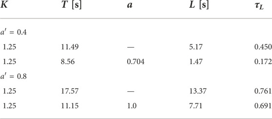
TABLE 2. FOPDT and SOPDT models.

5.2 SRT controller parameters and regulatory control performance

The SRT PI_eD_y2 controller parameters for four target robustness levels $M_S^t$ using the FOPDT and the SOPDT controlled process models are listed in Table 3 for the process with the time constant ratio a′ = 0.4 and in Table 4 for the process with a′ = 0.8. These tables also include the obtained control system robustness $M_S^m$ and the regulatory control behavior—performance J_ed and controller output total variation TV_ud. The control system robustness $M_S^m$ is evaluated using the controlled process low-order models Eqs. 25, 26, in a real industrial application, and it cannot be obtained directly with the controlled process. However, the system performance in terms of J_ed and TV_ud is evaluated with the original processes Eq. 24 as it may correspond to an application of the tuned controller and the corresponding recording of the closed-loop signals.

TABLE 3

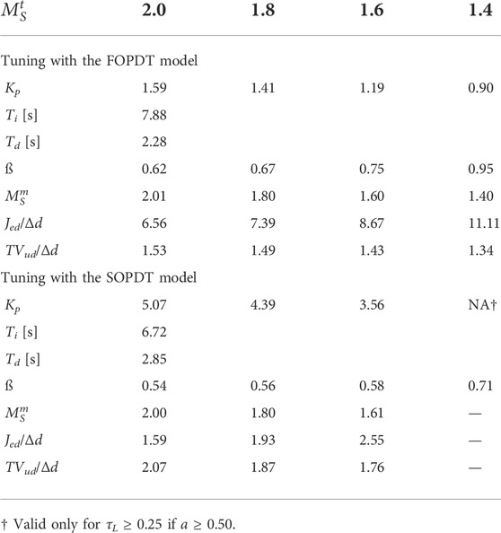
TABLE 3. SRT PI_eD_y2 controllers; process with a′=0.4

TABLE 4

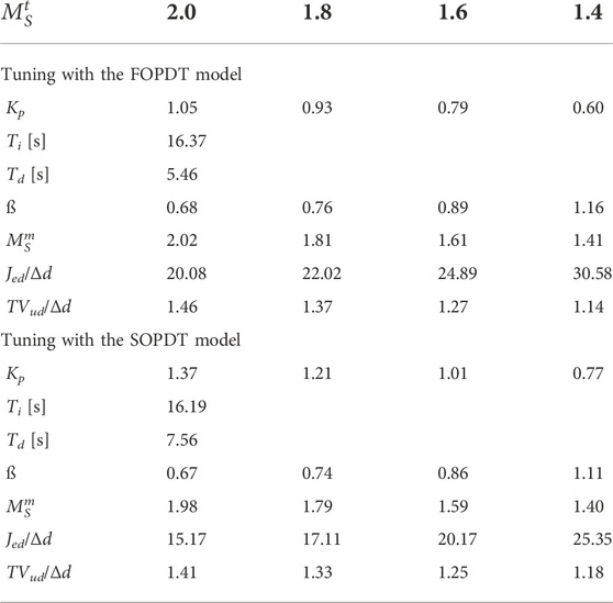
TABLE 4. SRT PI_eD_y2 controllers; process with a′ = 0.8

Regarding the achieved robustness and its effects on the control system performance, the first thing noticed in these tables is that all the controllers—based on four different models—achieve the target robustness levels within 1%. It is also noticed that an inverse relation exists between the control system robustness and its performance. If the target robustness is increased $-M_S^t\downarrow -$, the control system performance decreases—J_ed ↑—but the control effort is smoother—J_ud ↓. There is a conflict between the control system robustness and its performance, but it cannot be considered an industrial control system design tradeoff. The control system design robustness level is process-dependent. It is a requirement imposed by the controlled process non-linearity—changes in the process dynamic characteristics in the control system operation range. Then, the required control system robustness level is a must and its performance should be sacrificed.

As all the controllers considered—PI_eD_y2, PI_eD_y1, and I_ePD_y1—have the same feedback controller transfer function Eq. 11, their closed-loop regulatory control transfer functions as well as their robustness and performance are all the same as listed in Tables 3, 4. In fact, robustness is a feedback property, and having the same closed-loop regulatory control transfer functions, the three controller implementations provide the same robustness.

For both controlled processes—a ∈ {0.4, 0.8}—two low-order models were obtained—FOPDT and SOPDT—and used for tuning purposes. From the control system evaluation, it is clear that for the same robustness level, the control systems designed using the SOPDT models provide better performance, but with a less smooth control effort, than the corresponding systems designed using the FOPDT models.

From the designer’s point of view, the marginal extra effort needed to obtain a SOPDT low-order model to represent the controlled process in the controller design procedure pays for itself with the higher performance obtained. The regulatory control responses for the process Eq. 24 with a′ = 0.4 are shown in Figure 3. It shows the robustness/performance conflict, but more important is the performance increase obtained by designing the control system using the SOPDT model instead of the FOPDT one. As a complementary view of the better regulatory capabilities, we can look at the integral gain. This is defined as K_i = K_p/T_i. We can observe that larger values are obtained for designs based on an SOPDT process model. Therefore, better capacity of the controller is needed to reduce the load disturbance effect.

FIGURE 3

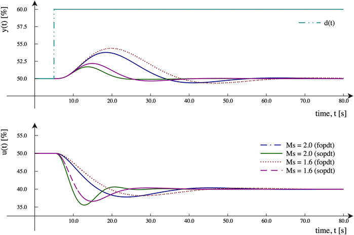
FIGURE 3. Regulatory control responses, when a′ = 0.4.

5.3 SRT servo-control performance

The obtained servo-control performance with the three different controllers for the controlled process with a′ = 0.4 is listed in Table 5—tuned with the FOPDT model—and in Table 6—tuned with the SOPDT model.

TABLE 5

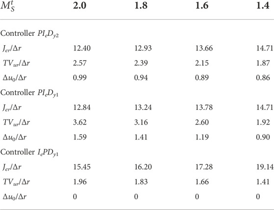
TABLE 5. Servo-control response; process with a′ = 0.4 and tuning using the FOPDT model.

TABLE 6

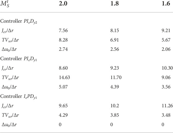
TABLE 6. Servo-control response; process with a′ = 0.4 and tuning using the SOPDT model.

Corresponding performance data for the controlled process with a′ = 0.8 are listed in Table 7 (FOPDT) and in Table 8 (SOPDT).

TABLE 7

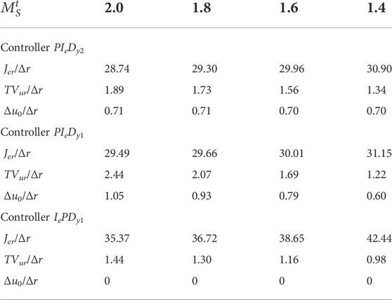
TABLE 7. Servo-control response; process with a′ = 0.8 and tuning using the FOPDT model.

TABLE 8

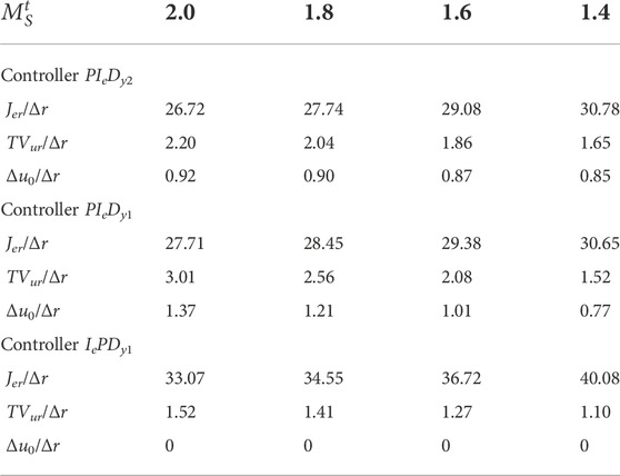
TABLE 8. Servo-control response; process with a′ = 0.8 and tuning using the SOPDT model.

As in PI_eD_y1 and I_ePD_y1 controllers, the second degree of freedom of the PI_eD_y2 controller is lost, and its servo-control performance is lower than the performance obtained with the latter. As shown in Table 1, the PI_eD_y1 controller is equivalent to a PI_eD_y2 controller with ß = 1, and the I_ePD_y1 controller is equivalent to a PI_eD_y2 controller with ß = 0. The drop in the servo-control performance obtained using the 1-DoF controllers depends on the controlled process, the model used for controller tuning, and its target robustness level can be related with the proportional set-point weight factor ß.

For the controlled processes used for the evaluation, the set-point weight factor ß-values vary from 0.54 to 1.16. Then, as the required ß-value approaches 1.0, the PI_eD_y1 servo-control performance losses decrease, but the performance corresponding to the I_ePD_y1 controller increases (this implementation corresponds to a ß = 0 2-DoF controller).

The SRT proportional set-point weight factor ß as a function of the normalized model dead-time τ_L = L/T and the different robustness target levels $M_S^t$ are shown in Figure 4. As for all models ß > 0.50, the servo-control performance lost with a PI_eD_y1 controller is lower than the one lost with an I_ePD_y1 controller. A performance reduction in the tracking operation is therefore expected. Some of the robust servo-control responses (a′ = 0.4, $M_S^t=1.6$) are shown in Figure 5. For a given robustness level, the PI_eD_y2 controller output is “optimal”—has the lowest J_er. The I_ePD_y1 controller loses 22% less performance than the PI_eD_y2 controller, but its control effort is smoother—has the lowest TV_ur and, more importantly, has no proportional “kick”—Δu₀ = 0.

FIGURE 4

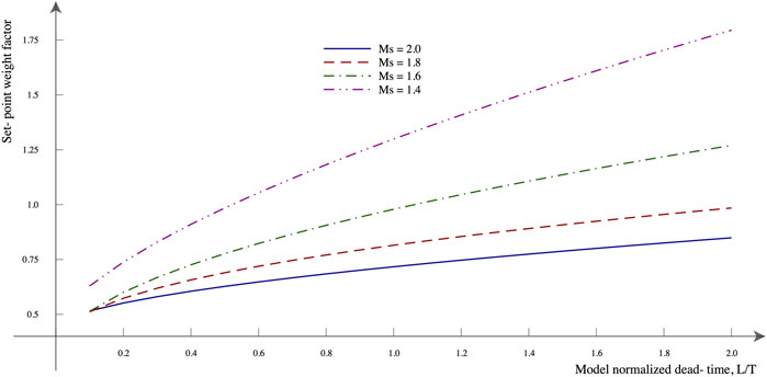
FIGURE 4. SRT proportional set-point weight factor.

FIGURE 5

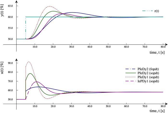
FIGURE 5. Servo-control responses, when a′ = 0.4 and $M_S^t=1.6$.

5.4 Robust I_ePD_y tuning performance

To the best of the authors’ knowledge, the method proposed by Vilanova et al. (2018b) is one of the few robust tuning procedures available specifically designed for I_ePD_y1 controllers. Herein, it is denoted as the VAGG method. It optimizes the I_ePD_y1 control system servo-control response—using the IAE cost functional—assuring at the same time a specific robustness level—M_S ∈ {2.0 (tight), 1.6 (smooth)}—for FOPDT-controlled process models. The VAGG controller parameters and performance indices for the controlled process Eq. 24 using models Eq. 25 are listed in Table 9.

TABLE 9

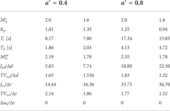
TABLE 9. VAGG robust I_ePD_y tuning.

As it can be noticed, the obtained closed-loop control system robustness $(M_S^m)$ is in the range of 6.25%–11.5% lower than the corresponding target levels. Therefore, the resulting control system is less robust than expected. Then, to have a fair comparison, the VAGG controller proportional gains K_p are reduced in the range of 8%–15%—without changing the controller integral times T_i and derivative times T_d—to increase the control system robustness up to the target levels. The new controller’s proportional gains $K_p^{*}$ and the performance obtained are listed in Table 10.

TABLE 10

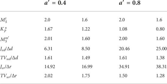
TABLE 10. VAGG robust I_ePD_y tuning with reduced gain.

The VAGG I_ePD_y1 controller performances are very similar to the ones obtained with the FOPDT model-based SRT I_ePD_y1 controllers, ΔJ_ex% ∈ [ − 3.8 ⋯ + 1.9], and with smoother control efforts but not better than the ones obtained with the SOPDT model-based SRT I_ePD_y1 controllers. Then, additional investigation is needed on the performance of the robustly tuned I_ePD_y1 controllers using SOPDT models to see if a new tuning rule is needed or if one of the existing optimal and robust regulatory control tunings for 1-DoF or 2-DoF PI_eD_y controllers can be used with an I_ePD_y1 controller without a significant loss of performance⁴.

5.5 Servo-control performance for a controlled variable with noise

As a complementary evaluation, additional controller performance tests are conducted for a controlled process variable corrupted with a measurement noise. The servo-control normalized performances J_ern for five simulation runs, and their averages values are listed in Table 11 for different controller configurations. The servo responses for a noisy signal (Run 2) are shown in Figure 6. As the change in the controller configurations is relevant for what matters to the tracking operation, the load disturbance is not evaluated or shown here. We can see that the effect of the noise with respect to the ideal situation can be considered negligible. Table 6 shows the values obtained in the ideal case.

TABLE 11

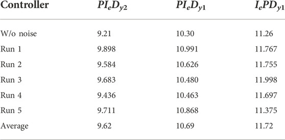
TABLE 11. Servo-control performance J_er/Δr (a′ = 0.4, SOPDT model, and $M_S^t=1.6$).

FIGURE 6

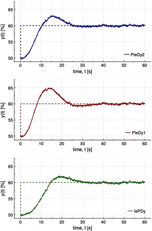
FIGURE 6. Servo-control, controlled variable w/noise (Run 2), a′ = 0.4, SOPDT model, and $M_S^t=1.6$.

6 Discussion

The previous section provided the performance evaluation of the SRT under different scenarios. It is evident that the comparison is process- and robustness-dependent. However, some general conclusions can be drawn.

According to the performance measures shown in Tables 5, 6, it is possible to evaluate the performance loss with respect to the following two implementation changes:

• PI_eD_y2 → PI_eD_y1: In this case, the second degree of freedom is lost, and a 2-DoF-tuned controller is implemented in a 1-DoF form. If we evaluate the performance losses and the corresponding PFI_Δ, it turns out that they are <0.1 for all tunings carried out using an FOPDT model. Therefore, we face resilient tuning. For the design concurred with a better SOPDT model, the PFI_Δ is also <0.1 for the process with a′ = 0.4 and slightly higher than 0.1 for a′ = 0.8 but in any case far from 0.5. Therefore, we can say that SRT tuning is resilient and non-fragile.

• PI_eD_y2 → I_ePD_y1: As we move to I_ePD_y1 implementation, the change is more drastic because just the integral term processes the reference signal. Therefore, a larger performance drop is expected for reference changes. In fact, in this case, for both FOPDT and SOPDT-based tuning, the resulting PFI_Δ is very similar: slightly greater than 0.2 but in any case far from 0.5. Therefore, we can say that SRT tuning is non-fragile.

The previous classification of the SRT rule as resilient in almost all cases is a rather qualitative evaluation that, in any case, provides an idea of the low sensitivity of the tuning with respect to the implementation of the reference processing term. It is important to bear in mind here that when tuning the three (or four in the 2-DoF case) parameters of a PID controller, distribution of the controller gain is carried out among the different parameters. Therefore, assigning how those gains take care of the two essential signals that do generate the error: the reference signal—for tracking purposes—and the feedback signal—for regulation purposes—altered because of potential disturbances. Depending on how those gains are distributed, the loss of performance in one of the operating modes can be really higher. Therefore, even qualitatively, the fact that the SRT tuning rule is almost in all cases resilient stands as a proof of a balanced gain distribution.

If we focus on a more quantitative evaluation, the only option is to compare the achieved performance on the implemented configuration with respect to a tuning designed specifically for such controller implementation. In this respect, we conducted an evaluation of the VAAG tuning (Vilanova et al., 2018b) performance. As this is a tuning optimized for the I_ePD_y1 controller implementation and includes at the same time robustness considerations, it provides a perfect scenario to quantitatively evaluate the degraded performance of the SRT tuning.

Table 10 shows the VAAG performance for a fair comparison. For the two robustness levels considered in Vilanova et al. (2018b), as observed in the previous subsection, the results show that the performance of an I_ePD_y1 controller tuned with the VAGG is very similar to the one obtained with the FOPDT model-based SRT (even SRT is not originally optimized for I_ePD_y1). If we start with SOPDT model-based SRT tuning, in this case, even the SRT’s degraded performance is better than the one achieved by the VAAG. This quantitative evaluation raises the question about the potential interpretation of the previously categorized non-fragility of SOPDT-based SRT tuning as really resilient with respect to structural changes in the controller implementation.

7 Conclusion

This work has presented a position work regarding the importance of the PID controller structure. Most of the tuning rules are conceived for a PID controller where the reference signal is processed by both the integral and the proportional term (either with or without a reference weighting factor).

One of the major drawbacks of the basic parallel formulations of the PID controllers is the effects of proportional and derivative kick. The changes in the set-point cause an impulse signal or a sudden change in the controller output as well as the output response. The controller output is given to the final control elements like control valve, motor, or electronic circuit in which the spikes create serious problems. In order to minimize these effects, modified forms of parallel controller structures such as PI-D and I-PD are usually considered in practice. Therefore, it turns out that tuning may finally be applied to an I-PD controller.

The considered simple robust tuning (SRT) allows to tune a PI/PID controller for an FOPDT as well as an SOPDT process model. The advantages of using a better process model have been outlined, and the use of SOPDT models instead of FOPDT models is greatly encouraged. This fact may allow minimizing the loss of performance when the final implementation is an I-PD instead of a PID as usual. This fact will make the tuning rule resilient with respect to the PID implementation.

This issue is not usually considered when presenting new tuning rules or when comparing with existing, well-established tunings. Modern tunings use approaches driven by advanced multi-objective algorithms that provide the final tuning values for the controller parameters. The optimality of such a design is not discussed at all. However, other more practical constraints should also be taken into account. This is a similar situation as the one with the fragility of tuning (Alfaro, 2007). Fragility and resilience, taken together, are concepts of great utility for the final practitioner as this will generate more confidence into the provided tuning.

In this work, only simple robust tuning was evaluated as an example. The purpose was to present a situation where a robust design based on FOPDT and SOPDT process models can be evaluated with respect to different PID controller implementations—PI_eD_y2, PI_eDy1, and I_ePD_y1. This helped shed light on the robustness/performance tradeoff, effect of the process model, and loss of performance because of controller implementation, as well as quite different evaluation issues that are not usually taken into account.

Data availability statement

The original contributions presented in the study are included in the article/Supplementary Material; further inquiries can be directed to the corresponding authors.

Author contributions

All authors listed have made a substantial, direct, and intellectual contribution to the work and approved it for publication.

Funding

This work received support from the Catalan government under project 2017 SGR 1202 and also by the Spanish government under project PID 2019-105434RBC33 co-funded by the European Union ERDF.

Conflict of interest

The authors declare that the research was conducted in the absence of any commercial or financial relationships that could be construed as a potential conflict of interest.

Publisher’s note

All claims expressed in this article are solely those of the authors and do not necessarily represent those of their affiliated organizations, or those of the publisher, the editors, and the reviewers. Any product that may be evaluated in this article, or claim that may be made by its manufacturer, is not guaranteed or endorsed by the publisher.

Footnotes

¹A second degree of freedom is understood here as the separate processing of the reference signal, usually with a set-point weight ß that modifies the usual error signal e = r − y to e = βr − y.

²M_S is the well-known robustness measure of the closed-loop system in terms of the maximum sensitivity function $M_S\dot{=}{\max }_{\omega }\left|\frac{1}{1+C(jw)P(jw)}\right|$.

³Derivative filter constant α = 0.1 is used in all controllers.

⁴For example, the RoPe tuning method (Alfaro et al., 2011).

References

Alcantara, S., Vilanova, R., and Pedret, C. (2013). PID control in terms of robustness/performance and servo/regulator trade-offs: A unifying approach to balanced autotuning. J. Process Control 23, 527–542. doi:10.1016/j.jprocont.2013.01.003

CrossRef Full Text | Google Scholar

Alfaro, V. M., and Vilanova, R. (2012a). “Conversion formulae and performance capabilities of two-degree-of-freedom pid control algorithms,” in Proceedings of 2012 IEEE 17th International Conference on Emerging Technologies Factory Automation (ETFA), Krakov, Poland, September 17–September 21, 2012, 1–6.

CrossRef Full Text | Google Scholar

Alfaro, V. M., and Vilanova, R. (2012b). “Chap. Fragility evaluation of PI and PID controllers tuning rules,” in PID control in the third millenium - lessons learned and new approaches (Springer-Verlag London Limited), 349–380.

CrossRef Full Text | Google Scholar

Alfaro, V. M., and Vilanova, R. (2013). Simple robust tuning of 2DoF PID controllers from a performance/robustness trade-off analysis. Asian J. Control 15, 1700–1713. doi:10.1002/asjc.653

CrossRef Full Text | Google Scholar

Alfaro, V. M., and Vilanova, R. (2016). “Model-reference robust tuning of PID controllers,” in Advances in industrial control series (Springer-Verlag).

CrossRef Full Text | Google Scholar

Alfaro, V. M., Méndez, V., and Vilanova, R. (2011). “Robust-performance tuning od 2DoF PI/PID controllers for first- and second-order-plus-dead-time models,” in 9th IEEE International Conference on Control & Automation (ICCA11), Santiago, Chile, December 19-21.

Google Scholar

Alfaro, V. M. (2006). Low-order models identification from the process reaction curve, (In Spanish). Cienc. Tecnol. (Costa Rica) 24 (2), 197–216. Available at https://revistas.ucr.ac.cr/index.php/cienciaytecnologia/article/view/2647/2598.

Google Scholar

Alfaro, V. M. (2007). PID controllers’ fragility. ISA Trans. 46, 555–559. doi:10.1016/j.isatra.2007.03.006

PubMed Abstract | CrossRef Full Text | Google Scholar

Ang, K. H., Chong, G., and Li, Y. (2005). Pid control system analysis, design, and technology. IEEE Trans. Control Syst. Technol. 13, 559–576. doi:10.1109/tcst.2005.847331

CrossRef Full Text | Google Scholar

Åström, K. J., and Hägglund, T. (2000). “Benchmark systems for PID control,” in IFAC Digital Control: Past, Present and Future of PID Control (PID’00), Terrasa, Spain, 5-7 April.

Google Scholar

Åström, K. J., and Hägglund, T. (2006). “Advanced PID control,” in ISA - The instrumentation, systems, and automation society.

Google Scholar

Bennett, S. (1993). Development of the pid controller. IEEE Control Syst. Mag. 13, 58–62. doi:10.1109/37.248006

CrossRef Full Text | Google Scholar

Chien, I., Hrones, J., and Reswick, J. (1952). On the automatic Control of generalized passive systems. J. Fluids Eng. 74, 175–183. doi:10.1115/1.4015724

CrossRef Full Text | Google Scholar

Johnson, M. A. (2005). “Chap. PID control technology,” in PID control - new identification and design methods (U.K: Springer-Verlag London Ltd.), 1–46.

Google Scholar

Minorsky, N. (1922). Directional stability of automatically steered bodies. J. Am. Soc. Nav. Eng. 34, 280–309. doi:10.1111/j.1559-3584.1922.tb04958.x

CrossRef Full Text | Google Scholar

O’Dwyer, A. (2009). Handbook of PI and PID controller tuning rules. 3rd. edn. London, UK: Imperial College Press.

Google Scholar

Ogawa, M., and Kano, M. (2008). Practice and challenges in chemical process control applications in Japan. IFAC Proc. Vol. 41, 10608–10613. doi:10.3182/20080706-5-kr-1001.01797

CrossRef Full Text | Google Scholar

Rivera, D. E., Morari, M., and Skogestad, S. (1986). Internal model control: PID controller design. Ind. Eng. Chem. Proc. Des. Dev. 25, 252–265. doi:10.1021/i200032a041

CrossRef Full Text | Google Scholar

Shinskey, F. G. (2002). Process control:as taught vs as practiced. Ind. Eng. Chem. Res. 41, 3745–3750. doi:10.1021/ie010645n

CrossRef Full Text | Google Scholar

Skogestad, S. (2003). Simple analytic rules for model reduction and PID controller tuning. J. Process Control 13, 291–309. doi:10.1016/s0959-1524(02)00062-8

CrossRef Full Text | Google Scholar

Vilanova, R., Santín, I., and Pedret, C. (2017). Control and operation of wastewater treatment plants (I). Rev. Iberoam. Autom. Inform. Ind. RIAI 14, 217–233. doi:10.1016/j.riai.2017.05.004

CrossRef Full Text | Google Scholar

Vilanova, R., Arrieta, O., Gonzalez, R., and Garrido, X. (2018a). I-pd controller as an structural alternative to servo/regulation tradeoff tuning. IFAC-PapersOnLine 51, 787–792. doi:10.1016/j.ifacol.2018.06.200

CrossRef Full Text | Google Scholar

Vilanova, R., Arrieta, O., González, R., and Garrido, X. G. (2018b). I-PD controller as an structural alternative to servo/regulation tradeoff tuning. IFAC-PapersOnLine 51, 787–792. doi:10.1016/j.ifacol.2018.06.200

CrossRef Full Text | Google Scholar

Vilanova, R. (2008). Imc based robust PID design: Tuning guidelines and automatic tuning. J. Process Control 18, 61–70. doi:10.1016/j.jprocont.2007.05.004

CrossRef Full Text | Google Scholar

Ziegler, J. G., and Nichols, N. B. (1942). Optimum settings for automatic controllers. Trans. ASME 64, 759–768.

Google Scholar