Competitive perimeter defense with a turret and a mobile vehicle

1 Introduction

With ever-expanding capabilities of Unmanned Aerial Vehicles (UAVs) and ground robots, collectively known as autonomous agents, it is now possible to deploy a team of autonomous agents for critical tasks such as surveillance (Ma’sum et al., 2013; Tavakoli et al., 2012), exploration (Howard et al., 2006; Koveos et al., 2007), and patrolling (Kappel et al., 2020). Although homogeneous agents can be used in such applications, a team of heterogeneous autonomous agents can outperform homogeneous autonomous agents because of the different capabilities of the agents and thus, there has been a considerable interest in employing heterogeneous autonomous agents for such applications (Santos and Egerstedt, 2018; Ramachandran et al., 2019; Ramachandran et al., 2021). A critical application for such autonomous agents is defending a region (commonly known as perimeter) such as airports, wildlife habitats, or a military facility from intrusive UAVs or poachers (Casey, 2014; Lykou et al., 2020) motivating fundamental algorithmic research for perimeter defense applications using heterogeneous defenders.

In this work, we address a perimeter defense problem in a conical environment. The environment contains two heterogeneous defenders, namely a turret and a mobile vehicle, which seek to defend a perimeter by capturing mobile intruders. The intruders are released at the boundary of the environment and move radially inwards with fixed speed toward the perimeter. Defenders have access to intruder locations only after they are released in the environment. Further, the defenders have distinct motion and capture capability and thus, are heterogeneous in nature. Specifically, the vehicle, having a finite capture radius, moves with unit speed in the environment whereas the turret has a finite range and can only turn clockwise or anti-clockwise with a fixed angular rate. Jointly, the defenders aim to capture as many intruders as possible before they reach the perimeter. This is an online problem as the input, which consists of the total number of intruders, their release locations, as well as their release times, is gradually revealed over time to the defenders. Thus, we focus on the design and analysis of online algorithms to route the defenders. Aside from military applications, this work is also motivated by monitoring applications wherein a drone and a camera jointly monitor the crowd entering a stadium.

Introduced in (Isaacs, 1999) as a target guarding problem, perimeter defense problem is a variant of pursuit evasion problems in which the aim is to determine optimal policies for the pursuers (or vehicles) and evaders (or intruders) by formulating it as a differential game. Versions with multiple vehicles and intruders have been studied extensively as reach-avoid games (Chen et al., 2016; Yan et al., 2018; Yan et al., 2019) and border defense games (Garcia et al., 2019; Garcia et al., 2020) and generally focus on a classical approach which requires computing solutions to the Hamilton-Jacobi-Bellman-Isaacs equation. However, this approach, due to the curse of dimensionality, is applicable only for low dimensional state spaces and simple environments (Margellos and Lygeros, 2011). Another work (Lee et al., 2020) addresses a class of perimeter defense problems, called perimeter defense games, which require the defenders to be constrained on the perimeter. We refer the reader to (Shishika and Kumar, 2020) for a review of perimeter defense games. Other recent works include (Guerrero-Bonilla et al., 2021) and (Lee and Bakolas, 2021) which consider an approach based on control barrier function or a convex shaped perimeter, respectively. All of these works consider mobile agents or vehicles that can move in any direction in the environment. Recently, (Akilan and Fuchs, 2017) considered a turret as a defender and introduced a differential game between a turret and a mobile intruder with an instantaneous cost based on the angular separation between the two. A similar problem setup with the possibility of retreat was considered in (Von Moll and Fuchs, 2020; Von Moll and Fuchs, 2021). Further, (Von Moll et al., 2022a) and (Von Moll et al., 2022b) considered a scenario in which the turret seeks to align its angle to that of the intruders in order to neutralize an attacker. All of these works assume that some information about the intruders is known a priori and do not consider heterogeneous defenders.

Online problems which require that the route of the vehicle be re-planned as information is revealed gradually over time are known as dynamic vehicle routing problems (Psaraftis, 1988; Bertsimas and Van Ryzin, 1991; Bullo et al., 2011). In these problems, the input (also known as demands) is static and therefore, the problem is to find the shortest route through the demands in order to minimize (maximize) the cost (reward). Examples of such metrics would be the total service time or the number of inputs serviced. In perimeter defense scenarios, the input (intruders) are not static. Instead, they are moving towards a specified region, making this problem more challenging than the former. With the assumption that the arrival process of the intruders is stochastic (Smith et al., 2009; Bajaj and Bopardikar, 2019; Macharet et al., 2020), consider the perimeter defense problem, in a circular or rectangular environment, as a vehicle routing problem using a single defender or multiple but homogeneous defenders. Recently (Adler et al., 2022) considered a problem of perimeter defense wherein either all of the attackers are known to the defenders at time 0 or the attackers are generated (i) uniformly randomly or (ii) by an adversary and determine how fast each defender must be in order to defend the perimeter. Although, in this work we consider worst-case scenarios, which is equivalent to the intruders being generated by an adversary, the speed of the defenders is fixed and we focus on designing cooperative online algorithms for the defenders. Other related works that do not make any assumptions on the intruders are (McGee and Hedrick, 2006; Francos and Bruckstein, 2021). However in these works, the aim is to design must-win algorithms, i.e., algorithms that detect every intruder in an environment.

Most prior works on perimeter defense problems have only considered defenders with identical capabilities. Further, they have either focused on determining an optimal strategy for scenarios with either few intruders or intruders generated by a stochastic process. The optimal strategy approaches do not scale with an arbitrary number of intruders released online. While stochastic approaches yield important insights into the average-case performance of defense strategies, they do not account for the worst-case in which intruders may coordinate their arrival to overcome the defense.

This work considers a perimeter defense problem with two heterogeneous defenders and focuses on worst-case instances. In particular, we establish fundamental guarantees as well as design online algorithms and provide analytical bounds on their performance in the worst-case. To evaluate the performance of online algorithms in the worst-case when faced with arbitrarily many intruders, we adopt a competitive analysis perspective (Sleator and Tarjan, 1985) which has also been studied in robotic exploration (Deng and Mirzaian, 1996), searching (Ozsoyeller et al., 2013), and design of state-space controllers (Sabag et al., 2022). Under this paradigm, an online algorithm $\mathcal{A}$’s performance is measured using the notion of competitive ratio: the ratio of the optimal (possibly non-causal) algorithm’s performance and algorithm $\mathcal{A}$’s performance for a worst-case input sequence for algorithm $\mathcal{A}$. An algorithm is c-competitive if its competitive ratio is no larger than c, which means its performance is guaranteed to be within a factor c of the optimal, for all input sequences.

Previously, we introduced the perimeter defense problem for a single defender in linear environments using competitive analysis (Bajaj et al., 2021). This was followed by (Bajaj et al., 2022c), which are the conference version of this current paper and focused on the perimeter defense problem for a single vehicle and a single turret in conical environments, respectively. The main contributions of this work are as follows:

• Perimeter defense problem with heterogeneous defenders: We address a perimeter defense problem in a conical environment with two cooperative heterogeneous defenders, i.e., a vehicle and a turret, tasked to defend a perimeter. The vehicle has a finite capture radius and moves with unit speed, whereas the turret has a finite engagement range and turns in the environment with a fixed angular rate. We do not impose any assumption on the arrival process of the intruders. More precisely, an arbitrary number of intruders can be released in the environment at arbitrary locations and time instances. Upon release, the intruders move with fixed speed v towards the perimeter. Thus, the perimeter defense problem is characterized by six parameters: (i) angle θ of the conical environment, (ii) the speed v of the intruders, (iii) the perimeter radius ρ, (iv) the engagement range of the turret r_t, (v) the angular rate of the turret ω, and (vi) the capture radius of the vehicle r_c.

• Necessary condition: We establish a necessary condition on the existence of any c-competitive algorithm for any finite c. This condition serves as a fundamental limit to this problem and identifies regimes for the six problem parameters in which this problem does not admit an effective online algorithm.

• Algorithm Design and Analysis: We design and analyze four classes of cooperative algorithms with provably finite competitive ratios under specific parameter regimes. Specifically, the first two cooperative algorithms are provably 1-competitive, the third cooperative algorithm exhibits a finite competitive ratio which depends on the problem parameters and finally, the fourth algorithm is 1.5-competitive.Additionally, through multiple parameter regime plots, we shed light into the relative comparison and the effectiveness of our algorithms. We also provide a brief discussion on the time complexity of our algorithms and how this work can be extended to other models of the vehicle.The paper is organized as follows. In Section 2, we formally define the competitive ratio and our problem. Section 3 establishes the necessary conditions, Section 4 presents the algorithms and their analysis. Section 5 provides several numerical insights. Finally, Section 7 summarizes the paper and outlines future directions.

2 Problem formulation

Consider a planar conical environment (Figure 1) described by $\mathcal{E}(\theta )=\{(y,\alpha ):0<y\le 1,-\theta \le \alpha \le \theta \}$, where (y, α) denotes a location in polar coordinates. The environment has two endpoints, (1, θ) and (1, − θ). The environment contains a concentric and coaxial region, $\mathcal{R}$, described by a set of points (z, α) in polar coordinates, where 0 < z ≤ ρ and α ∈ [−θ, θ]. Mathematically, $\mathcal{R}(\rho ,\theta )=\{(z,\alpha ):0<z\le \rho <1,-\theta \le \alpha \le \theta \}$ for some ρ ∈ (0, 1). Analogous to the environment, $\mathcal{R}$’s endpoints are (ρ, θ) and (ρ, − θ). Arbitrary numbers of intruders are released at the circumference of the environment, i.e., y = 1, at arbitrary time instants. Upon release, each intruder moves radially inward with a fixed speed v > 0¹ toward the perimeter $\partial \mathcal{R}(\theta )=\{(\rho ,\alpha ):-\theta \le \alpha \le \theta \}$. Mathematically, if the ith intruder is released at time t_i, then its location is represented by a constant angle θ_i and its distance $z_i^t$ from the origin satisfying $z_i^t=1-v(t-t_i),\forall t\in [t_i,t_i+(1-\rho )/v]$. Two defenders are employed to defend the perimeter, $\partial \mathcal{R}$ of the region $\mathcal{R}(\rho ,\theta )$: a turret located at the origin of $\mathcal{E}(\theta )$ and a vehicle, both with simple motion dynamics. The vehicle has a finite capture radius, r_c > 0 and can either move with unit speed or remain stationary. The turret has a finite engagement range, r_t such that ρ ≤ r_t ≤ 1, and can either turn clockwise or anti-clockwise with an angular speed of at most ω or remain stationary. We consider that the vehicle’s capture radius is sufficiently small, in particular, r_c < min{ρ, ρ tan(θ)}. Otherwise, this problem becomes trivial (refer to (Bajaj et al., 2022c)).

FIGURE 1

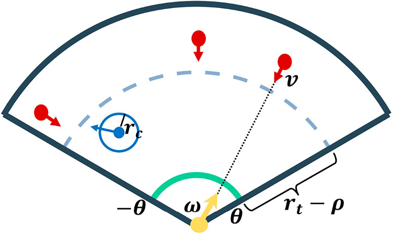
FIGURE 1. Problem Description. The vehicle is depicted by a blue dot and the blue circle around the vehicle depicts the capture circle. The direction of the vehicle is shown by the blue arrow. The yellow arrow depicts the turret (located at the origin of $\mathcal{E}(\theta )$) and the blue dashed curve denotes the engagement range of the turret. The green curve denotes the perimeter and the red dots denote the intruders. Note that the intruder that the turret is pointing to (black dashed line) is not captured unless it is within the engagement range of the turret (blue dashed curve).

Intruder i, located at $(z_i^t,{\theta }_i)$, is said to be captured at time instant t if either one of the following holds:

• intruder i is inside or on the capture circle of the mobile vehicle at time t, or

• intruder i is at most r_t distance away from the origin and γ_t = θ_i holds, where γ_t denotes the heading of the turret at time instant t.

The intruder is said to be lost by the defenders if it reaches the perimeter without getting captured. The intruder is removed from $\mathcal{E}(\theta )$ if it is either captured or lost. We assume that the turret and the vehicle neutralize an intruder instantaneously, i.e., they do not require any additional service time. This implies that the defenders do not need to stop to complete the capture of an intruder. We further assume that the turret can start and stop firing instantaneously. This implies that the turret does not neutralize the vehicle in case the turret’s heading angle is the same as the vehicle’s angular coordinate at a particular time instant.

A problem instance $\mathcal{P}$ is characterized by six parameters: (i) the speed of the intruders v > 0, (ii) the perimeter radius 0 < ρ < 1, (iii) the angle 0 < θ ≤ π that defines the size of the environment as well as the perimeter, (iv) the capture radius of the vehicle 0 < r_c < min{ρ, ρ tan(θ)}, (v) the angular speed of the turret ω > 0, and (vi) the range of the turret ρ ≤ r_t ≤ 1. An input sequence $\mathcal{I}$ is a set of 3-tuples comprising: (i) an arbitrary time instant t ≤ T, where T denotes the final time instant, (ii) the number of intruders N(t) that are released at time instant t, and (iii) the release location (radius and angle) of each of the N(t) intruders. Formally, $\mathcal{I}={\{t,N(t),\{(1,{\alpha }_1),(1,{\alpha }_2),\dots ,(1,{\alpha }_{N(t)})\}\}}_{t=0}^T$, for any α_l ∈ [−θ, θ], where 1 ≤ l ≤ N(t).

An online algorithm $\mathcal{A}$ assigns velocities with unit (resp. at most ω) magnitude to the vehicle (resp. turret) at time t as a function of the input $I(t)\subset \mathcal{I}$ revealed until time t. An optimal offline algorithm is an algorithm which has complete information of the entire input sequence $\mathcal{I}$ a priori to assign velocities to the vehicle and the turret at any time t. The performance of an online algorithm as well as the optimal offline algorithm for a problem instance $\mathcal{P}$ is the total number of intruders captured by the vehicle and by the turret out of an input sequence $\mathcal{I}$. Let $n_{\mathcal{A}}(\mathcal{I},\mathcal{P})$ (resp. $n_{\mathcal{O}}(\mathcal{I},\mathcal{P})$) denote the performance of an online algorithm $\mathcal{A}$ (resp. optimal offline algorithm $\mathcal{O}$) on an input sequence $\mathcal{I}$. Then, we define the competitive ratio as the following.

Definition 1 (Competitive Ratio): Given a problem instance $\mathcal{P}$, an input sequence $\mathcal{I}$, and an online deterministic algorithm $\mathcal{A}$, the competitive ratio of $\mathcal{A}$ for the input sequence $\mathcal{I}$ is defined as $C_{\mathcal{A}}(\mathcal{I},\mathcal{P})≔\frac{n_{\mathcal{O}}(\mathcal{I},\mathcal{P})}{n_{\mathcal{A}}(\mathcal{I},\mathcal{P})}\ge 1$, and the competitive ratio of $\mathcal{A}$ for the problem instance $\mathcal{P}$ is $c_{\mathcal{A}}(\mathcal{P})={\sup }_{\mathcal{I}}{C}_{\mathcal{A}}(\mathcal{I},\mathcal{P})$. Finally, the competitive ratio for the problem instance $\mathcal{P}$ is $c(\mathcal{P})={\inf }_{\mathcal{A}}{c}_{\mathcal{A}}(\mathcal{P})$. An online algorithm is c-competitive for the problem instance $\mathcal{P}$ if, for all input sequences $\mathcal{I}$, $n_{\mathcal{A}}(\mathcal{I},\mathcal{P})\le c{n}_{\mathcal{O}}(\mathcal{I},\mathcal{P})+\bar{c}$ holds, where c ≥ 1 and $\bar{c}\ge 0$ are fixed constants.

The constant $\bar{c}$ is sometimes used to account for the initial differences in the state of the online and the optimal offline algorithm and is generally insignificant for longer initial input sequences. In this work, we use the strict definition of competitive ratio, i.e., $\bar{c}=0$. More formally, we say that an online algorithm is c-competitive for the problem instance $\mathcal{P}$ if, for all input sequences $\mathcal{I}$, $n_{\mathcal{A}}(\mathcal{I},\mathcal{P})\le c{n}_{\mathcal{O}}(\mathcal{I},\mathcal{P})$ holds. However, we will see later that all of our results also hold for $\bar{c}>0$ as well. We refer (Borodin and El-Yaniv, 2005) for further details on the definition of c-competitive algorithms.

Competitive analysis falls under a general framework of Request-Answer games and thus, can be viewed as a game between an online player and an adversary (Borodin and El-Yaniv, 2005). An adversary is defined as a pair $(\mathcal{Q},\mathcal{O})$, where $\mathcal{Q}$ is the input component responsible for generating the input sequences $\mathcal{I}$ and $\mathcal{O}$ is an optimal offline algorithm which maximizes $n_{\mathcal{O}}(\mathcal{I},\mathcal{P})$. Thus, the adversary, with the information of the online algorithm, constructs a worst-case input sequence so as to maximize the competitive ratio, i.e., it minimizes the number of intruders captured by the online algorithm and simultaneously maximizes the number of intruders captured by an optimal offline algorithm. On the other hand, the online player operates an online algorithm on an input sequence created by the adversary. In this work, we restrict the choice of inputs $\mathcal{I}$ to those for which there exists an optimal offline algorithm $\mathcal{O}$ such that $n_{\mathcal{O}}(\mathcal{I},\mathcal{P})\ge 1$. Clearly, $n_{\mathcal{O}}(\mathcal{I},\mathcal{P})\ge n_{\mathcal{A}}(\mathcal{I},\mathcal{P})$. However, if for some $\mathcal{I}$, $n_{\mathcal{A}}(\mathcal{I},\mathcal{P})=0$, then we say that $\mathcal{A}$ is not c-competitive for any finite c. We now formally define the objective of this work.

Problem Statement: Design online deterministic cooperative algorithms with finite competitive ratios for the defenders and establish fundamental guarantees on the existence of online algorithms with finite competitive ratio.

We start by determining a fundamental limit on the existence of c-competitive algorithms followed by designing online cooperative algorithms.

3 Fundamental limits

We start by defining a partition of the environment. A partition of $\mathcal{E}(\theta )$ is a collection of q ≥ 1 cones $\mathcal{W}=\{W_1,W_2,\dots ,W_q\}$ with disjoint interiors and whose union is $\mathcal{E}(\theta )$. Additionally, each cone is of unit radius having a finite positive angle and is concentric with the environment. We refer to a cone W_m, 1 ≤ i ≤ q as the mth dominance region. Further, an endpoint of a dominance region is defined analogously as the endpoints of the environment. Given any set of initial locations of the defenders with distinct angular coordinates, the environment $\mathcal{E}(\theta )$ can be partitioned into two dominance regions such that each dominance region corresponds to a particular defender. We denote the portion of the perimeter contained in dominance region m, 1 ≤ m ≤ 2, as ∂R_m. Without loss of generality, we assume that $\partial {\mathcal{R}}_1$ (resp. $\partial {\mathcal{R}}_2$) corresponds to the leftmost (resp. rightmost) dominance region.

Let f₁(α) = 2ω(ρ sin(α) − r_c) + α − θ and f₂(α) = 0.5ω(ρ sin(α) − r_c) + α − θ. Let ${\bar{\alpha }}_1$ denote the solution to the equation f₁(α) = 0 and let ${\bar{\alpha }}_2$ be the solution to the equation f₂(α) = 0. Then, following result establishes a necessary condition on the existence of c-competitive algorithms.

Theorem 3.1: (Necessary Condition for finite $c_{\mathcal{A}}(\mathcal{P})$). Let

${\alpha }_1^{*}=\left\{\begin{array}{cc}\theta -2\omega \left(\rho -r_c\right),\hfill & \mathit{\text{i}}\mathit{\text{f}}\theta \ge \frac{\pi }{2}+2\omega \left(\rho -r_c\right),\hfill \\ {\bar{\alpha }}_1,\hfill & otherwise,\hfill \end{array}\right.$

and let

${\alpha }_2^{*}=\left\{\begin{array}{cc}\theta -0.5\omega \left(\rho -r_c\right),\hfill & \mathit{\text{i}}\mathit{\text{f}}\theta \ge \frac{\pi }{2}+\omega \left(\rho -r_c\right),\hfill \\ {\bar{\alpha }}_2,\hfill & otherwise.\hfill \end{array}\right.$

Then, for any problem instance $\mathcal{P}$ such that ρ sin(θ) > r_c and $\frac{v}{\omega }>\frac{1-\rho }{\min \{\theta -{\alpha }_1^{*},2(\theta -{\alpha }_2^{*})\}}$ holds, there does not exist a c-competitive algorithm for any finite c.

Proof. Recall from Definition 1 that any online algorithm $\mathcal{A}$ is c-competitive if the condition $n_{\mathcal{O}}(\mathcal{I},\mathcal{P})\le c{n}_{\mathcal{A}}(\mathcal{I},\mathcal{P})$ holds for every input sequence $\mathcal{I}$. Thus, the aim is to construct an input sequence $\mathcal{I}$ such that the condition $n_{\mathcal{O}}(\mathcal{I},\mathcal{P})\le c{n}_{\mathcal{A}}(\mathcal{I},\mathcal{P})$ does not hold for any constant c ≥ 1 regardless of which online algorithm is used. The proof is in three parts. First, we construct an input sequence $\mathcal{I}$. Then, we determine the best locations for the defenders against such an input sequence. Finally, we evaluate the performance of any online algorithm $\mathcal{A}$ on the input $\mathcal{I}$ as well as the performance of the optimal offline algorithm $\mathcal{O}$ on the same input sequence $\mathcal{I}$, to establish the result. Without loss of generality, we assume that both $\mathcal{A}$ and $\mathcal{O}$ have the vehicle at the origin at time instant 0 and the turret at angle γ₀ = 0.

Let $\mathbf{I}=\{{\mathcal{I}}_1,{\mathcal{I}}_2\}$ denote a set of two input sequences. Each input sequence ${\mathcal{I}}_l\in \mathbf{I}$, where l ∈ {1, 2}, differs in the location of the arrival of intruders. Both input sequences ${\mathcal{I}}_1$ and ${\mathcal{I}}_2$ start at time instant $\max \{1,\frac{\theta }{\omega }\}$ and consists of a stream of intruders, i.e., a sequence of a single intruder arriving at location (1, θ) at every time instant $\max \{1,\frac{\theta }{\omega }\}+k\frac{1-\rho }{v},k\in \mathbb{N}\cup \{0\}$ until time instant t. The time instant t ≥ 0 corresponds to the time instant when either the vehicle or the turret, following any online algorithm $\mathcal{A}$, captures an intruder from the stream. A burst of c + 1 intruders are then released at time instant t. The location where the burst of intruder arrives is different for each input sequence ${\mathcal{I}}_l,l\in \{\mathrm{1,2}\}$. Given the location of the turret and the vehicle at time instant t, there can be at most two dominance regions of the environment and thus, at most two locations where the burst of intruders can arrive. These locations have the same angular coordinate as the endpoints of each ∂R_m, ∀m ∈ {1, 2} excluding θ and including −θ. Without loss of generality, the burst of intruders are released at location (1, − θ) for ${\mathcal{I}}_1$. Further, if the heading angle of the turret is the same as the angular coordinate of the vehicle at time t, i.e., γ_t = θ and the vehicle’s angular coordinate is θ at time instant t, then the burst intruders arrive at (1, − θ) for both ${\mathcal{I}}_1$ and ${\mathcal{I}}_2$ (In this case, ${\mathcal{I}}_1$ is same as ${\mathcal{I}}_2$).

If neither the vehicle nor the turret captures the stream intruder, the stream never ends and the result follows as the optimal offline algorithm $\mathcal{O}$ can have its vehicle move, at time instant 0, to location (ρ, θ) and capture all stream intruders. Thus, in the remainder of the proof, we only consider online algorithms $\mathcal{A}$ for which either the vehicle or the turret captures at least one stream intruder at time instant t. Since the stream intruders arrive every $\frac{1-\rho }{v}$ time units apart and stops when an intruder from the stream is captured, it follows that no online algorithm can capture more than one intruder from the stream. Thus, we assume that the ith stream intruder was captured at time instant t, for some $i\in {\mathbb{Z}}_{+}$, where ${\mathbb{Z}}_{+}$ denotes the set of positive integers.

We now determine the best locations, or equivalently the dominance regions of the environment, for the turret and the vehicle at time instant t. Note that the heading angle of the turret must not be equal to the angular coordinate of the vehicle at time instant t. This is because in such case, the burst arrives at (1, − θ) and thus, there always exist a location closer to angle −θ such that the vehicle or the turret can reach angular location −θ in less time. This implies that at time instant t, the environment consists of two dominance regions, each of which contains a defender. We denote the dominance region which contains the vehicle (resp. turret) as W_Veh (resp. W_Tur) and determine them in the following two cases. These two cases arise based on whether the vehicle or the turret captures the ith intruder, each of which is considered below.

Case 1 (Vehicle captures the ith intruder): Let 2α₁ and 2β₁ be the angles of W_Veh and W_Tur, respectively. The best location for the vehicle and the turret in this case can be summarized as follows. The vehicle must be located on the line joining the two endpoints of the perimeter within its W_Veh $(\partial {\mathcal{R}}_2)$ only if 2α₁ < π. Otherwise, vehicle must be located on the line joining the origin to the location (1, θ). In both cases, it must be at a distance r from location (ρ, θ). The angle of the turret must be equal to the angle bisector of 2β₁ (Figure 2A). Finally, the time taken by the vehicle to reach the other endpoint of $\partial {\mathcal{R}}_2$ must be equal to the time taken by the turret to turn to the same angle corresponding to that location. This is denoted mathematically as

$\frac{\theta -{\alpha }_1}{\omega }=\left\{\begin{array}{c}2\left(\rho \sin \left({\alpha }_1\right)-r_c\right)\text{\hspace{0.17em}if\hspace{0.17em}}{\alpha }_1<\frac{\pi }{2}\hfill \\ 2\left(\rho -r_c\right),\text{\hspace{0.17em}otherwise}\hfill \end{array}\right.(1)$

where by definition 2θ = 2α₁ + 2β₁ and the time taken by the vehicle to capture intruders at the other endpoint of the perimeter contained in its dominance region is 2(ρ sin(α₁) − r_c) (resp. 2(ρ − r_c)) when ${\alpha }_1<\frac{\pi }{2}$ (resp. ${\alpha }_1\ge \frac{\pi }{2}$). As $\frac{\theta -{\alpha }_1}{\omega }=2(\rho -r_c)$ only holds if ${\alpha }_1\ge \frac{\pi }{2}$, it follows that ${\alpha }_1^{*}=\theta -2\omega (\rho -r_c)$ if $\theta \ge \frac{\pi }{2}+2\omega (\rho -r_c)$ holds. Otherwise, ${\alpha }_1^{*}$ is determined by solving the equation f₁(α) = 0, where f₁(α) = 2ω(ρ sin(α) − r_c) + α − θ where ${\alpha }_1\in \left[0,\pi /2\right)$. We now show that the solution to f₁(α) = 0 always exist if r_c < ρ sin(θ).

Suppose that α₁ = ϵ, where ϵ > 0 is a very small number. Then, f(ϵ) = 2ωρ sin(ϵ) + ϵ − θ − 2r_cω < 0. Now consider that α₁ = θ − ϵ for the same ϵ. Then, as ρ sin(θ) > r_c, it follows that f₁(θ − ϵ) = 2ω(ρ sin(θ − ϵ) − r_c) − ϵ > 0, for a sufficiently small ϵ. This means that for a sufficiently small ϵ > 0, f₁(⋅) changes its sign in the interval [ϵ, θ − ϵ]. Thus, from Intermediate Value Theorem and using the fact that f₁(α₁) is continuous function of α₁, it follows that there must exist an ${\alpha }_1^{*}$ such that $f_1({\alpha }_1^{*})=0$ if r_c < ρ sin(θ). Further, since f₁(α) is a continuous function and its derivative is strictly increasing for $\alpha \in \left[0,\frac{\pi }{2}\right)$ and hence, there exists a unique ${\bar{\alpha }}_1\in \left[0,\frac{\pi }{2}\right)$ which satisfies f₁(α).

FIGURE 2

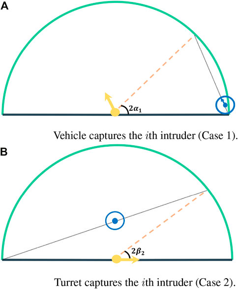
FIGURE 2. Depiction of the perimeter depicting the two cases under which one of the defenders captures the ith intruder. (A) Vehicle captures the ith intruder (Case 1). (B) Turret captures the ith intruder (Case 2).

Case 2 (Turret captures the ith intruder): Similar to Case 1, let 2α₂ and 2β₂ be the angles of W_Veh and W_Tur, respectively (Figure 2B). As the turret captures the stream intruder, it follows that γ_t = θ. Further, the vehicle must be located at the midpoint of the line joining the two endpoints of the perimeter within its dominance region. Finally, the time taken by the vehicle to reach any endpoint of the perimeter must be equal to the time taken by the turret to turn to the same angle corresponding to that location. Mathematically, this yields

$\frac{2\left(\theta -{\alpha }_2\right)}{\omega }=\left\{\begin{array}{c}\rho \sin \left({\alpha }_2\right)-r_c,\text{\hspace{0.17em}if\hspace{0.17em}}{\alpha }_2<\frac{\pi }{2}\hfill \\ \left(\rho -r_c\right),\text{\hspace{0.17em}otherwise}\hfill \end{array}\right.(2)$

where we used the fact that 2θ = 2α₂ + 2β₂ and ρ sin(α₂) − r_c (resp. (ρ − r_c)) denotes the time taken by the vehicle to capture intruders at the other endpoint of the perimeter contained in its dominance region when ${\alpha }_2<\frac{\pi }{2}$ (resp. ${\alpha }_2\ge \frac{\pi }{2}$). As $2\frac{\theta -{\alpha }_2}{\omega }=(\rho -r_c)$ only holds if ${\alpha }_2\ge \frac{\pi }{2}$, it follows that ${\alpha }_2^{*}=\theta -0.5\omega (\rho -r_c)$ if $\theta \ge \frac{\pi }{2}+0.5\omega (\rho -r_c)$ holds. Otherwise, ${\alpha }_2^{*}$ is determined by solving the equation f₂(α) = 0, where f₂(α) = 0.5ω(ρ sin(α) − r_c) + α − θ. By following similar steps as in Case 1, it can be shown that a unique solution to f₂(α) = 0 always exists if r_c < ρ sin(θ) and thus, has been omitted for brevity.

As $\frac{1-\rho }{v}<\min \{2(\rho \sin ({\alpha }_1^{*})-r_c),\rho \sin ({\alpha }_2^{*})-r_c\}$ or equivalently $v>\frac{1-\rho }{\min \{2(\rho \sin ({\alpha }_1^{*})-r_c),\rho \sin ({\alpha }_2^{*})-r_c\}}$ holds for ${\alpha }_1^{*}<\frac{\pi }{2}$, it follows that the vehicle cannot capture the burst intruders from ${\mathcal{I}}_2$ or ${\mathcal{I}}_1$. Further, as $2(\rho \sin ({\alpha }_1^{*})-r_c)=\frac{\theta -{\alpha }_1^{*}}{\omega }$ or $\rho \sin ({\alpha }_2^{*})-r_c=\frac{2(\theta -{\alpha }_2^{*})}{\omega }$ holds at time instant t, it follows that the turret can also not capture the burst intruders from both ${\mathcal{I}}_1$ and ${\mathcal{I}}_2$. Therefore, the turret and the vehicle jointly captures at most one intruder from input instance ${\mathcal{I}}_1$ as well as ${\mathcal{I}}_2$. A similar conclusion holds when ${\alpha }_1^{*}\ge \frac{\pi }{2}$ or when ${\alpha }_2^{*}\ge \frac{\pi }{2}$.

Thus, we have established that for any online algorithm $\mathcal{A}$, the vehicle and the turret can jointly capture at most a single intruder from input instance ${\mathcal{I}}_l,1\le l\le 2$. We now show that the optimal offline algorithm $\mathcal{O}$ captures all of the intruders on the input sequence ${\mathcal{I}}_l,1\le l\le 2$.

Recall that $\mathcal{O}$ has complete information at time 0, of when, where, and how many intruders will arrive. Thus, at time 0, $\mathcal{O}$ moves its vehicle to location (ρ, θ) and the turret to angle −θ. The defenders of $\mathcal{O}$ have sufficient time to reach these locations as the first intruder arrives at time instant $\max \{1,\frac{\theta }{\omega }\}$ and thus, the capture of all i stream intruders as well as the burst intruders is guaranteed. Thus, $n_{\mathcal{O}}(\mathcal{I},\mathcal{P})=i+c+1$ and $n_{\mathcal{A}}(\mathcal{I},\mathcal{P})=1$ which yields that $\frac{n_{\mathcal{O}}(\mathcal{I},\mathcal{P})}{n_{\mathcal{A}}(\mathcal{I},\mathcal{P})}=i+c+1$. As i + c + 1 > c for any constant c, it follows that $n_{\mathcal{O}}(\mathcal{I})\le c{n}_{\mathcal{A}}(\mathcal{I})$ does not hold for any c. This concludes the proof.

Remark 3.2: Since we do not impose any restriction on the number of intruders that can arrive in the environment, an adversary can repeat the input sequence designed in the proof of Theorem 3.1 any number of times. Thus, the lower bound derived in Theorem 3.1 holds asymptotically for when $\bar{c}>0$ in the definition of c-competitive algorithms as well.

We now turn our attention to designing online algorithms and deriving upper bounds on their competitive ratios. In the next section, we design and analyze four online algorithms, each with a provably finite competitive ratio in a specified parameter regime.

4 Online algorithms

In this section, we design and analyze online algorithms and characterize the parameter space in which these algorithms have finite competitive ratios. The parameter space of all of our algorithms is characterized by two main quantities:

• The time taken by the intruders to reach the perimeter in the worst-case and

• the time taken by the defenders to complete their respective motions.

Intuitively, the parameter space is obtained by comparing the aforementioned quantities². Since the time taken by the intruders is inversely proportional to v, the (v, ρ) parameter space of our algorithms can be increased by designing the algorithms such that the time taken by the defenders to complete their motions is the least. We characterize the time taken by the defenders to complete their respective motions as epochs, which is formally defined as follows.

An epoch k for an algorithm is defined as the time interval which begins when at least one of the two defenders moves from its initial position and ends when both defenders return back to their respective initial positions. We denote the time instant when an epoch k begins as k_s.

We now describe our first algorithm that has the best possible competitive ratio.

Algorithm 1. Sweep within Dominance Region Algorithm

1 Turret is at angle −θ

2 if α = arctan($r_c/\rho$) then

3    Vehicle is located at (ρ/cos(α) , θ − α)

4    for each epoch k do

5      Turn the turret clockwise to angle θ − 2α

6      Turn the turret anti-clockwise to angle −θ

7    end

8  else

9    Vehicle is located at ($z_v$, θ)

10    for each epoch k do

11      Turn vehicle (resp. turret) anti-clockwise (resp. clockwise) until it reaches location (resp. angle) ($z_v$, θ − 2α) (resp. θ − 2α)

12      Turn vehicle (resp. turret) clockwise (resp. anti-clockwise) until it reaches location (resp. angle) ($z_v$, θ) (resp. −θ)

13    end

14  end

4.1 Sweep within dominance region (SiR)

Algorithm SiR is an open-loop and memoryless algorithm in which we constrain the vehicle to move in an angular motion, i.e., either clockwise or anti-clockwise. This can be achieved by moving the vehicle with unit speed in the direction perpendicular to its position vector (see Figure 3A). By doing so, we aim to understand the worst-case scenarios for heterogeneous defenders and gain insights into the effect of the heterogeneity that arises due to the capture range of the defenders, i.e., the capture circle and the engagement range of the turret. We say that a defender sweeps in its dominance region if it turns, from its starting location, either clockwise or anti-clockwise to a specified location and then turns back to its initial location. Algorithm SiR is formally defined in Algorithm 1 and is summarized as follows.

FIGURE 3

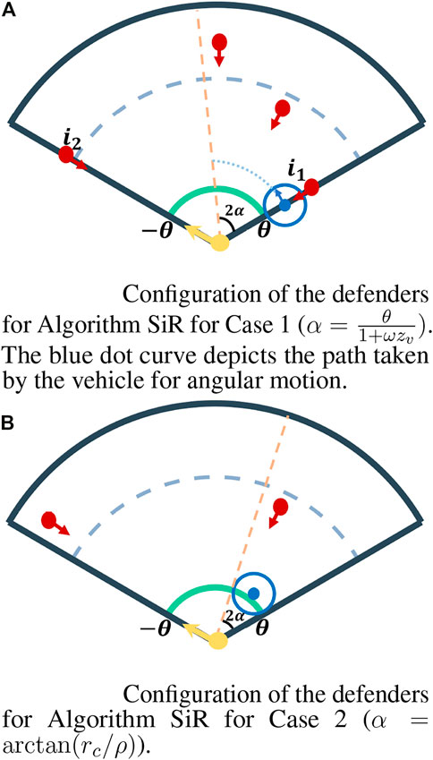
FIGURE 3. Partition (shown by the orange line) of the environment and the configuration of the defenders for the two cases of Algorithm SiR. (A) Configuration of the defenders for Algorithm SiR for Case 1 ($\alpha =\frac{\theta }{1+\omega z_v}$). The blue dot curve depicts the path taken by the vehicle for angular motion. (B) Configuration of the defenders for Algorithm SiR for Case 2 ($\alpha =\arctan (r_c/\rho )$).

Algorithm SiR first partitions the environment $\mathcal{E}(\theta )$ into two dominance regions and assigns a single defender to a dominance region. Let 2α denote the angle of W_Veh. Then, the vehicle takes exactly 4αz_v to sweep within its dominance region, where z_v denotes the radial location of the vehicle and will be determined shortly (see Case 1 below). Similarly, as the turret can only turn either clockwise or anti-clockwise with at most angular speed ω, the turret takes exactly $\frac{4(\theta -\alpha )}{\omega }$ to sweep in its respective dominance region W_Tur. Observe that the environment must be partitioned such that the time taken by the defenders to complete their motion in their respective dominance region is equal. Otherwise, in the worst-case, all of the intruders will be concentrated in the dominance region of that defender that takes more time to sweep its dominance region. Mathematically, this means $4\alpha z_v=\frac{4(\theta -\alpha )}{\omega }$ must hold which yields that $\alpha =\frac{\theta }{1+\omega z_v}$. Observe that as ω → ∞, α → 0. This means that the turret sweeps the entire environment, in time $\frac{4\theta }{\omega }$, if ω is sufficiently high. Recall that the (v, ρ) parameter space is characterized by the time taken by the defenders to complete their motion and can be improved by reducing the time taken by the turret, for high values of ω. In case of very high ω, this can be achieved by having the vehicle remain static at a specific location while the turret sweeps the remaining environment as opposed to the entire environment. This means that although angle $\alpha =\frac{\theta }{1+\omega z_v}$ characterizes the vehicle’s dominance region, there exists an angle $\widehat{\alpha }\ge \alpha$ for some values of problem parameters for which we can obtain an improved parameter regime by assigning a dominance region of angle $2\widehat{\alpha }$ to the vehicle. Thus, in Algorithm SiR, there are two cases based on the values of the problem parameters. First, as described above, the defenders sweep the environment in their respective dominance regions and second, the vehicle remains static at a specific location while the turret sweeps its dominance region. In what follows, we determine the location at which the vehicle must remain static for the second case, followed by formally describing the two cases.

The vehicle’s location must be such that its capture circle covers the perimeter contained in its dominance region entirely, ensuring that any intruder that arrives in that dominance region is guaranteed to be captured. To achieve this, the boundary of the dominance region assigned to the vehicle must be tangent to its capture circle (see Figure 3B) which, through geometry, yields that $\widehat{\alpha }=\arctan \frac{r_c}{\rho }$ and the location for the vehicle as $(\frac{\rho }{\cos (\widehat{\alpha })},\theta -\widehat{\alpha })$. Therefore, the angle of the vehicle’s dominance region is defined as $2\alpha =2\max \{\frac{\theta }{1+\omega z_v},\widehat{\alpha }\}$, where $\widehat{\alpha }=\arctan \frac{r_c}{\rho }$, and angle α determines if the vehicle sweeps in its dominance region or remains stationary. We first describe the motion of the turret followed by formally describing the motion of the vehicle in the two cases.

At time instant 0, the turret is at an angle −θ. The turret turns clockwise, with angular speed ω towards angle θ − 2α. Upon reaching angle θ − 2α, the turret turns anti-clockwise towards angle −θ. Note that the turret takes exactly $\frac{4(\theta -\alpha )}{\omega }$ time to complete its motion in a particular epoch. We now describe the motion of the vehicle which can be summarized in two cases described as follows:

Case 1 $(\alpha =\frac{\theta }{1+\omega z_v})$: At time instant 0, the vehicle is located at (z_v, θ), where z_v = min{ρ + r_c, 1 − r_c} and was determined in (7) and was proved to be optimal in (4). The vehicle then moves anti-clockwise with unit speed in the direction perpendicular to its position vector until it reaches the location (z_v, θ − 2α). Then, the vehicle moves clockwise, with direction perpendicular to its position vector, until it reaches location (z_v, θ). Note that the vehicle takes exactly 4αz_v time to complete its motion in a particular epoch. Since α is chosen so that $4\alpha z_v=\frac{4(\theta -\alpha )}{\omega }$, the vehicle and the turret return to their respective initial locations at the same time instant, at which the next epoch begins.

Case 2 $(\alpha =\arctan (\frac{r_c}{\rho }))$: At time instant 0, the vehicle is located at $(z_v=\frac{\rho }{\cos (\alpha )},\theta -\alpha )$ and remains stationary at this location for the entire duration. In this case, the next epoch begins once the turret turns back to angle −θ.

The following result characterizes the parameter regime in which Algorithm SiR is 1-competitive.

Theorem 4.1: Algorithm SiR is 1-competitive for a set of problem parameters that satisfy

$v\le \left\{\begin{array}{cc}\min \left\{\frac{\left(r_t-\rho \right)\left(1+\omega z_v\right)}{4\theta z_v},\frac{\left(z_v+r_c-\rho \right)\left(1+\omega z_v\right)}{4\theta z_v}\right\}\hfill & \mathit{\text{i}}\mathit{\text{f}}\frac{\theta }{1+\omega z_v}>\arctan \left(r_c/\rho \right)\hfill \\ \frac{\left(r_t-\rho \right)\omega }{4\left(\theta -\arctan \left(r_c/\rho \right)\right)},\hfill & otherwise.\hfill \end{array}\right.$

Otherwise, Algorithm SiR is not c-competitive for any constant c.

Proof. Suppose that $\alpha =\frac{\theta }{1+\omega z_v}$. At the start of any epoch k, i.e., at time instant k_s, we assume that, in the worst-case, intruders i₁ and i₂ are located at (z_v + r_c + ϵ₁, θ) and (r_t + ϵ₂, − θ), respectively, where ϵ₁ and ϵ₂ are arbitrary small positive numbers (see Figure 3A). To ensure that the vehicle (resp. turret) does not lose any intruder, we require that the time taken by the vehicle (resp. turret) to return to location (resp. angle) (z_v, θ) (resp. −θ) must be less than the time taken by intruder i₁ (resp. i₂) to reach the perimeter. Formally, $\frac{r_t+{ϵ}_2-\rho }{v}\ge \frac{4(\theta -\alpha )}{\omega }$ and $\frac{z_v+r_c+{ϵ}_1-\rho }{v}\ge 4\alpha z_v$ must hold. Given the first condition on v, these two conditions always hold, so any intruder that arrives in the environment is guaranteed to be captured.

If $v>\min \{\frac{(r_t-\rho )(1+\omega z_v)}{4\theta z_v},\frac{(z_v+r_c-\rho )(1+\omega z_v)}{4\theta z_v}\}$, then there exists an input instance with intruders arriving only at (1, − θ) such that these intruders are located at (r_t + ϵ, − θ) at the time instant the turret turns from angle −θ. As $v>\min \{\frac{(r_t-\rho )(1+\omega z_v)}{4\theta z_v},\frac{(z_v+r_c-\rho )(1+\omega z_v)}{4\theta z_v}\}$ all of these intruders will be lost and thus, from Definition 1, Algorithm SiR will not be c-competitive.

Now consider that $\alpha =\arctan (\frac{r_c}{\rho })$. As the vehicle remains stationary in its dominance region and the location of the vehicle is such that no intruder that is released in that dominance region can reach the perimeter, we only focus on the turret. Assume that, in the worst-case, intruder i₁ is located at (r_t + ϵ, − θ) where ϵ is an arbitrary small positive numbers. To ensure that the turret does not lose any intruder, we require that the time taken by the turret to return to angle −θ must be less than the time taken by intruder i₁ to reach the perimeter. Given the second condition on v, i.e., $v\le \frac{(r_t-\rho )\omega }{4(\theta -\arctan (r_c/\rho ))}$ holds, it is ensured that intruder i₁ will be captured. The proof for Algorithm SiR not being c-competitive when $v>\frac{(r_t-\rho )\omega }{4(\theta -\arctan (r_c/\rho ))}$ is analogous to the previous case and has been omitted for brevity. This concludes the proof.

Although Algorithm SiR is 1-competitive, note that for r_t = ρ, the algorithm is not effective as Theorem 4.1 yields v ≤ 0. However, by allowing the vehicle to sweep the entire environment, it is still possible to capture all intruders for some small v > 0. This is addressed in a similar algorithm below.

4.2 Sweep in conjunction (SiCon)

At time instant 0, the turret is at angle θ and the vehicle is located at location (min{r_t + r_c, 1}, θ). The idea is to move the two defenders together in angular motion. Thus, the vehicle moves anti-clockwise with unit speed in the direction perpendicular to its position vector until it reaches the location (min{r_t + r_c, 1}, − θ). Similarly, the turret turns anti-clockwise, in conjunction with the vehicle, to angle −θ. Upon reaching −θ, the vehicle and the turret move clockwise until they reach angle θ. The defenders then begin the next epoch. As the two defenders move in conjunction, $\frac{2\theta }{\omega }=2\theta \min \{r_t+r_c,1\}\Rightarrow \omega =\frac{1}{\min \{r_t+r_c,1\}}$ must hold. Thus, this algorithm is effective for $\omega \ge \frac{1}{\min \{r_t+r_c,1\}}$ by turning the turret exactly with angular speed $\frac{1}{\min \{r_t+r_c,1\}}$.

The following result establishes that Algorithm SiCon is 1-competitive for specific parameter regimes.

Theorem 4.2: Algorithm SiCon is 1-competitive for a set of problem parameters which satisfy $\omega \ge \frac{1}{\min \{r_t+r_c,1\}}$ and $v\le \frac{\min \{r_t+2r_c,1\}-\rho }{4\theta \min \{r_t+r_c,1\}}$. Otherwise, it is not c-competitive for any constant c.

Proof. As the proof is analogous to the proof of Theorem 4.1, we only provide an outline of this proof for brevity. In the worst-case, an intruder requires exactly $\frac{\min \{r_t+2r_c,1\}-\rho }{v}$ time to reach the perimeter whereas, the defenders synchronously require 4θ min{r_t + r_c, 1} time to complete their motion in any epoch. Thus, as the time taken by the defenders must be at most the time taken by the intruders we obtain the competitive ratio. If the condition on v does not hold, then by constructing an input analogous to the input in the proof of Theorem 4.1, it can be shown that Algorithm SiCon is not c-competitive.

Remark 4.3: (Maneuvering Intruders). As the analysis of the fundamental limit (Theorem 3.1), Algorithm SiR, and Algorithm SiCon are independent of the nature of motion of the intruders, the results of Theorem 3.1, Algorithm SiR, and Algorithm SiCon apply directly to the case of maneuvering or evading intruders.

Recall that in Algorithm SiR, the idea was to partition the environment and assign a single defender in each dominance region. By doing so, we obtain valuable insight into the parameter regime wherein we are guaranteed to capture all intruders. However, we refrain from designing such algorithms in this work due to the following two reasons. First, such an algorithm requires that ratio of intruders captured by a defender to the total number of intruders that arrived in that corresponding defender’s dominance region is equal for both defenders. Otherwise, since the adversary has the information of the entire algorithm, it will release more intruders in the dominance region of the defender that has the lower ratio, which determines the competitive ratio of such an algorithm. Second, such algorithms are not cooperative and thus fall out of the scope of this paper. The objective of this work is to study how heterogeneous defenders can be used to improve the competitive ratio of a single defender. Thus, in the next algorithm, although we partition the environment, the defenders are not restricted to remain within their own dominance region.

Algorithm 2. Split and Capture Algorithm

1 Turret is at angle 0

2 Vehicle is located at (x₁, ϕ₁)

3 for each epoch k do

4   Compute $P_{\mathrm{r}\mathrm{i}\mathrm{g}\mathrm{h}\mathrm{t}}^k$, $P_{\mathrm{l}\mathrm{e}\mathrm{f}\mathrm{t}}^k$, $N_{p^{*}}$

5   if $P_{\mathrm{r}\mathrm{i}\mathrm{g}\mathrm{h}\mathrm{t}}^k$| ≥ |$P_{\mathrm{l}\mathrm{e}\mathrm{f}\mathrm{t}}^k$| then

6     Turn the turret clockwise to angle θ

7     Turn the turret back to angle 0

8   else

9     Turn the turret anti-clockwise to angle −θ

10     Turn the turret back to angle 0

11   end

12   if $N_{p^{*}}$ ≠ N_i then

13     if |$S_{{\mathrm{p}}^{*}}^{j+2}$| ≥ |$S_{\mathrm{i}}^{j+1}$ then

14       Move vehicle to $(x_{p^{*}},{\varphi }_{p^{*}})$ and then capture intruders in $S_{{\mathrm{p}}^{*}}^{j+2}$

15     else

16       Keep vehicle at (x_i, ϕ_i) and capture intruders in S^j+1_i

17       Move vehicle to $(x_{p^{*}},{\varphi }_{p^{*}})$

18     end

19   else

20     Keep vehicle at (x_i, ϕ_i) and capture intruders in $S_{\mathrm{i}}^{j+1}$ and $S_{\mathrm{i}}^{j+2}$

21   end

22 end

4.3 Split and capture (Split)

The motivation for this algorithm is to utilize the vehicle’s ability to move in any direction while the turret rotates either clockwise or anti-clockwise. Since the turret can only turn either clockwise or anti-clockwise, the idea is to first partition the environment into two-halves and turn the turret towards the side which has higher number of intruders. By doing so, we hope to capture at least half of the intruders by the turret, assuming they are sufficiently slow, that arrive in every epoch. Further, while the turret moves to capture intruders on one side, the vehicle moves to the other side to capture intruders, ensuring that the defenders jointly capture more than half of the intruders that arrive in the environment in every epoch. Algorithm Split is formally defined in Algorithm 2 and is summarized as follows where we first describe the motion of the turret in every epoch followed by that of the vehicle.

The heading angle of the turret is always ${\gamma }_{k_s}=0$ at the start of every epoch k. To determine whether the turret turns clockwise or anti-clockwise at time instant k_s, we first describe two sets P_left and P_right. These sets characterize a region on the left and right side of the y-axis, respectively, and are determined once at time instant 0.

$\begin{array}{ll}\hfill P_{\mathrm{r}\mathrm{i}\mathrm{g}\mathrm{h}\mathrm{t}}\left(\rho ,v\right)& ≔\left\{\left(y,\beta \right):\rho +\frac{\beta v}{\omega }<y\le \min \left\{1,r_t+\frac{\left(2\theta -\beta \right)v}{\omega }\right\},\forall \beta \in \left[0,\theta \right]\right\},\hfill \\ \hfill P_{\mathrm{l}\mathrm{e}\mathrm{f}\mathrm{t}}\left(\rho ,v\right)& ≔\left\{\left(y,\beta \right):\rho -\frac{\beta v}{\omega }<y\le \min \left\{1,r_t+\frac{\left(2\theta +\beta \right)v}{\omega }\right\},\forall \beta \in \left(0,-\theta \right]\right\}.\hfill \end{array}$

Let $P_{\mathrm{r}\mathrm{i}\mathrm{g}\mathrm{h}\mathrm{t}}^k$ and $P_{\mathrm{l}\mathrm{e}\mathrm{f}\mathrm{t}}^k$ denote the set of intruders contained in P_right and P_left (see Figure 4A), respectively, at the start of an epoch k and let |S| denote the cardinality of a set S of intruders. Then, at time instant k_s, the turret compares the total number of intruders in $P_{\mathrm{l}\mathrm{e}\mathrm{f}\mathrm{t}}^k$ to the total number of intruders in $P_{\mathrm{r}\mathrm{i}\mathrm{g}\mathrm{h}\mathrm{t}}^k$ and turns in the direction of the set which has higher number of intruders. More formally, if $|P_{\mathrm{r}\mathrm{i}\mathrm{g}\mathrm{h}\mathrm{t}}^k|<|P_{\mathrm{l}\mathrm{e}\mathrm{f}\mathrm{t}}^k|$ holds at time instant k_s, then the turret turns anti-clockwise towards angle −θ. Upon turning to angle −θ, the turret turns to angle 0. Otherwise, i.e., if $|P_{\mathrm{r}\mathrm{i}\mathrm{g}\mathrm{h}\mathrm{t}}^k|\ge |P_{\mathrm{l}\mathrm{e}\mathrm{f}\mathrm{t}}^k|$ holds at time instant k_s, then the turret turns clockwise towards angle θ. Upon turning to angle θ, the turret turns to angle 0. As the turret’s dominance region is determined at the start of every epoch k, we denote the turret’s dominance region as $W_{\mathrm{T}\mathrm{u}\mathrm{r}}^k$, and consequently, the other dominance region as the vehicle’s dominance region denoted as $W_{\mathrm{V}\mathrm{e}\mathrm{h}}^k$. We now characterize the motion for the vehicle which builds upon the SNP algorithm designed in (Bajaj et al., 2022).

FIGURE 4

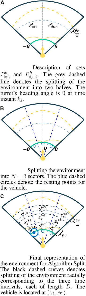
FIGURE 4. Description of Algorithm Split. The light grey dashed line denotes the splitting of the environment. The region between the yellow dashed curve and the yellow dot curve on the left (resp. right) side of the grey line denotes $P_{\mathrm{l}\mathrm{e}\mathrm{f}\mathrm{t}}^k$ (resp. $P_{\mathrm{r}\mathrm{i}\mathrm{g}\mathrm{h}\mathrm{t}}^k$). The blue dashed straight lines denote the sectors ($N=3$) of the environment and the black dashed curves denotes the three radial intervals of length $Dv$ each. The vehicle is located at $(x_1,{\varphi }_1)$. (A) Description of sets $P_{\mathrm{l}\mathrm{e}\mathrm{f}\mathrm{t}}^k$ and $P_{\mathrm{r}\mathrm{i}\mathrm{g}\mathrm{h}\mathrm{t}}^k$. The grey dashed line denotes the splitting of the environment into two halves. The turret's heading angle is $0$ at time instant $k_s$. (B) Splitting the environment into $N=3$ sectors. The blue dashed circles denote the resting points for the vehicle. (C) Final representation of the environment for Algorithm Split. The black dashed curves denotes splitting of the environment radially corresponding to the three time intervals, each of length $D$. The vehicle is located at $(x_1,{\varphi }_1)$.

Algorithm Split further divides the environment $\mathcal{E}(\theta )$ into $N=\lceil \frac{\theta }{{\theta }_s}\rceil$ sectors, where 2θ_s = 2 arctan(r_c/ρ) denotes the angle of each sector (see Figure 4B). The value 2 arctan(r_c/ρ) of the angle of each of the sectors is to ensure that the portion of the perimeter in a sector can be completely contained in the capture circle of the vehicle. This can be achieved by positioning the vehicle at resting points (see Figure 4B), which is a specific location in every sector and is formally defined as follows.

Definition 2 (Resting points). Let N_l denote the lth sector, for every l ∈ {1, …, N} where N₁ corresponds to the leftmost sector. Then, a resting point $(x_l,{\varphi }_l)\in \mathcal{E}(\theta )$ for sector N_l, is the location for the vehicle such that when positioned at (x_l, ϕ_l), the portion of the perimeter inside sector N_l is contained completely within the capture circle of the vehicle. Mathematically, this is equivalent to

$\left(x_l,{\varphi }_l\right)=\left(\frac{\rho }{\cos \left({\theta }_s\right)},\left(l-\frac{N+1}{2}\right)2{\theta }_s\right).$

Now, let D denote the distance between the two resting points that are furthest apart in the environment (see Figure 4B). Formally,

$D=\left\{\begin{array}{c}2\frac{\rho }{\cos \left({\theta }_s\right)}\sin \left(\left(N-1\right){\theta }_s\right),\text{\hspace{0.17em}if\hspace{0.17em}}\left(N-1\right){\theta }_s<\frac{\pi }{2},\hfill \\ 2\frac{\rho }{\cos \left({\theta }_s\right)},\text{\hspace{0.17em}otherwise.}\hfill \end{array}\right.(3)$

Observe that when N = 1, D = 0. This means that the vehicle captures all intruders that arrive in the environment by positioning itself to the unique resting point of the single sector.

Next, Algorithm Split radially divides the environment $\mathcal{E}(\theta )$ into three intervals of length Dv, corresponding to time intervals of time length D each (see Figure 4C). Specifically, the jth time interval for any j > 0 is defined as the time interval [(j − 1)D, jD]. Note that this time interval is different than the epoch of the algorithm. Let $S_l^j$ denote the set of intruders that are contained in the lth, l ∈ {1, …, N}, sector and were released in the jth interval. Then, at the start of each epoch, the motion of the vehicle is based on the following two steps: First, select a sector with the maximum number of intruders. Second, determine if it is beneficial to switch over to that sector. These two steps are achieved by two simple comparisons; C1 and C2 detailed below.

Suppose that the vehicle is located at the resting point of sector N_i at the start of the jth epoch and let $\tilde{\mathbf{N}}$ denote the set of sectors in the vehicle’s dominance region. Then, to specify the first comparison C1, we associate each sector $N_l\in \tilde{\mathbf{N}}$ with the quantity

${\eta }_i^l\triangleq \left\{\begin{array}{cc}|S_l^{j+2}|+|S_l^{j+3}|,\hfill & \text{if\hspace{0.17em}}l\ne i,\hfill \\ |S_i^{j+1}|+|S_i^{j+2}|+|S_i^{j+3}|,\hfill & \text{if\hspace{0.17em}}l=i.\hfill \end{array}\right.$

Note that ${\eta }_i^l$ is not defined for every sector in the environment. Instead, it is only defined for the sectors in $W_{\mathrm{V}\mathrm{e}\mathrm{h}}^j$, which may contain N_i. Then, as the outcome of C1, Algorithm Split selects the sector $N_{p^{*}}$, where $p^{*}={\mathrm{a}\mathrm{r}\mathrm{g}\mathrm{m}\mathrm{a}\mathrm{x}}_{p\in \tilde{\mathbf{N}}}{\eta }_i^p$. In case there are multiple sectors with same number of intruders, then Algorithm Split breaks the tie as follows. If the tie includes the current sector N_i (which is only possible if $N_i\in \tilde{\mathbf{N}}$ holds³), then Algorithm Split selects N_i. Otherwise, Algorithm Split selects the sector contained in $\tilde{\mathbf{N}}$ with the maximum number of intruders in the interval j + 2, i.e., $p^{*}={\mathrm{a}\mathrm{r}\mathrm{g}\mathrm{m}\mathrm{a}\mathrm{x}}_{p\in \widehat{\mathbf{N}}}|S_{\mathrm{p}}^{j+2}|$, where $\widehat{\mathbf{N}}$ denotes the set of sectors that have the same number of intruders. If this results in another tie, then this second tie is resolved by selecting the sector with the least index. Let the sector chosen as the outcome of C1 be N_o.

We now describe comparison C2 jointly with the motion of the vehicle in the following two points:

• If the sector chosen as the outcome of C1 is N_o, o ≠ i, and the total number of intruders in the set $S_o^{j+2}$ is no less than the total number of intruders in $S_i^{j+1}$, then Algorithm Split moves the vehicle to (x_o, ϕ_o) arriving in at most D time units. Then the vehicle waits at that location to capture all intruders in $S_o^{j+2}$. Otherwise, i.e., the total number of intruders in $S_o^{j+2}$ is less than $S_i^{j+1}$, then the vehicle stays at (x_i, ϕ_i) until it captures all of the intruders in $S_i^{j+1}$ and then moves to (x_o, ϕ_o) arriving in at most D time units.

• If the sector chosen is N_i, then the vehicle stays at its current location (x_i, ϕ_i) for 2D time units capturing intruders in $S_i^{j+1}$ and $S_i^{j+2}$.

Note that the vehicle takes at most 2D time units in every case above. The vehicle then re-evaluates after 2D time. At time instant 0, the turret’s heading angle is 0 and the vehicle is located at (x₁, ϕ₁). The first epoch begins when the first intruder arrives in the environment.

We now describe two key requirements for the algorithm. The first requirement is to ensure that the defenders start their individual motion in an epoch at the same time instant. Recall that the turret requires exactly $\frac{2\theta }{\omega }$ time to turn from its initial heading angle to either θ or −θ, at time instant k_s, and turn back to its initial heading angle. On the other hand, the vehicle requires 2D time units to capture intruders in at least one interval. Thus, to ensure that the defenders begin their motion at the same time instant, $\frac{2\theta }{\omega }=2D$ must hold, i.e., the speed of the turret must be at least $\frac{\theta }{D}$. The second requirement is to ensure that the algorithm has a finite competitive ratio. This is achieved by ensuring that any intruder that was not accounted for comparison by the defenders (for instance intruders that are not in $P_{\mathrm{l}\mathrm{e}\mathrm{f}\mathrm{t}}^k$ or $P_{\mathrm{r}\mathrm{i}\mathrm{g}\mathrm{h}\mathrm{t}}^k$) in an epoch k, are accounted in epoch k + 1. Our next result formally characterizes this requirement for the turret.

Lemma 4.4. Any intruder with radial coordinate greater than $\min \{1,r_t+\frac{(2\theta -\beta )v}{\omega }\},\forall \beta \in [0,\theta ]$ (resp. $\min \{1,r_t+\frac{(2\theta +\beta )v}{\omega }\},\forall \beta \in (0,-\left.\theta \right])$ at time instant k_s will be contained in the set $P_{\mathrm{r}\mathrm{i}\mathrm{g}\mathrm{h}\mathrm{t}}^{k+1}$ (resp. $P_{\mathrm{l}\mathrm{e}\mathrm{f}\mathrm{t}}^{k+1}$) at time instant (k + 1)_s if $v\le \frac{\omega (r_t-\rho )}{2\theta }$ holds.

Proof. Without loss of generality, suppose that $|P_{\mathrm{l}\mathrm{e}\mathrm{f}\mathrm{t}}^k|\le |P_{\mathrm{r}\mathrm{i}\mathrm{g}\mathrm{h}\mathrm{t}}^k|$ holds at time instant k_s. Then, the total time taken by the turret to move towards θ and turn back to angle 0 is $\frac{2\theta }{\omega }$. In order for any intruder i to not be captured in epoch k, in the worst-case, the intruder i must be located at (min{1, r_t} + ϵ, θ), where ϵ is a very small positive number, by the time the turret reaches angle θ. Note that 1 + ϵ here means that the intruder is released after ϵ time at location (1, θ) after the turret’s heading angle is θ. Thus, in order to ensure that i can be captured in epoch k + 1, the condition $\frac{2\theta }{\omega }\le \frac{r_t-\rho }{v}$ must hold, where we used the fact that r_t ≤ 1 and ϵ is a very small positive number. From the definition of $P_{\mathrm{r}\mathrm{i}\mathrm{g}\mathrm{h}\mathrm{t}}^k$, if the intruder i can be captured in epoch k + 1, then it follows that the intruder i was contained in the set $P_{\mathrm{r}\mathrm{i}\mathrm{g}\mathrm{h}\mathrm{t}}^{k+1}$ at the start of epoch (k + 1). This concludes the proof.

The proof of Lemma 4.4 is established in the worst-case scenario which is that an intruder, with angular coordinate θ (resp. −θ), is located just above the range of the turret at the time instant when the turret’s heading angle is θ (resp. −θ) in an epoch k. This is because in an epoch k, the angle θ is the only heading angle that is visited by the turret once as the turret turns to all angles $\beta \forall \beta \in \left[0,\theta \right)$ (resp. $\left[0,-\theta \right)$) twice; once when the turret turns to angle θ or −θ and second, when turret turns back to angle 0. This results in the following corollary, the proof of which is analogous to the proof of Lemma 4.4.

Corollary 4.5: Suppose that the turret moves to capture intruders in $P_{\mathrm{l}\mathrm{e}\mathrm{f}\mathrm{t}}^k$ (resp. $P_{\mathrm{r}\mathrm{i}\mathrm{g}\mathrm{h}\mathrm{t}}^k$) in epoch k. Then, the intruders contained in $P_{\mathrm{r}\mathrm{i}\mathrm{g}\mathrm{h}\mathrm{t}}^k$ (resp. $P_{\mathrm{l}\mathrm{e}\mathrm{f}\mathrm{t}}^k$) with radial coordinate strictly greater than $r_t+\frac{v\theta }{\omega }$ at time instant k_s will be considered for comparison at the start of epoch (k + 1) if $v\le \frac{\omega (r_t-\rho )}{2\theta }$.

Recall that the adversary selects the release times and the locations of the intruders in our setup. Thus, with the information of the online algorithm, the adversary can release intruders such that all the intruders have their radial coordinates at most $r_t+\frac{\theta v}{\omega }$ and at angular location θ of −θ at the start of every epoch k, which is considered to be the worst-case scenario. This ensures that if the turret selects to turn towards −θ (resp. θ) at time k_s, then the turret cannot capture any intruder that was contained in $P_{\mathrm{r}\mathrm{i}\mathrm{g}\mathrm{h}\mathrm{t}}^k$ (resp. $P_{\mathrm{l}\mathrm{e}\mathrm{f}\mathrm{t}}^k$) in epoch k + 1. As the idea is to have the vehicle capture these intruders, we require that the intruders must be sufficiently slow. This is explained in greater detail as follows.

For the vehicle, the requirement is that the intruders take at least 3D time units to reach the perimeter. This is to ensure that the vehicle can account for intruders that are very close to the perimeter at the start of an epoch. From Corollary 4.5, as the intruders with radial location greater than $r_t+\frac{\theta v}{\omega }$ are counted for comparison in next epoch by the turret, we require that these intruders must also be counted by the vehicle in the next epoch. This yields that $3D\le \frac{\min \{1,r_t+\frac{\theta v}{\omega }\}-\rho }{v}$ which implies that either $v\le \frac{1-\rho }{3D}$ or $v\le \frac{r_t-\rho }{2D}$ must hold, where we used the fact that $\frac{2\theta }{\omega }=2D$. Finally, as Lemma 4.4 requires that $v\le \frac{r_t-\rho }{2D}$ must hold, the second requirement for Algorithm Split is that $v\le \min \{\frac{1-\rho }{3D},\frac{r_t-\rho }{2D}\}$. We now establish the competitive ratio of Algorithm Split.

Theorem 4.6: Let θ_s = arctan(r_c/ρ) and $N=\lceil \frac{\theta }{{\theta }_s}\rceil$. Then, for any problem instance $\mathcal{P}$ with the turret’s angular velocity $\omega \ge \frac{\theta }{D}$, where D is defined in equation 3, Algorithm Split is $\frac{3N-1}{3\lfloor 0.5N\rfloor +2}$-competitive if $v\le \min \{\frac{1-\rho }{3D},\frac{r_t-\rho }{2D}\}$.

Proof. First observe that although the turret can capture intruders from one-half of the environment, the vehicle only captures at most two intervals out of all intervals that are in $W_{\mathrm{V}\mathrm{e}\mathrm{h}}^k$ (the total number of intervals in $W_{\mathrm{V}\mathrm{e}\mathrm{h}}^k$ will be determined shortly). Thus, in the worst-case, the intruders are released in the environment such that there are as many intruders possible in the vehicle’s dominance region. Since $W_{\mathrm{V}\mathrm{e}\mathrm{h}}^k$ is selected based on $W_{\mathrm{T}\mathrm{u}\mathrm{r}}^k$, there cannot be more number of intruders in the vehicle’s dominance region as than those in the turret’s dominance region. This implies that there are equal number of intruders in each dominance region in every epoch in the worst-case. We now characterize the total number of intervals in the vehicle’s dominance region.

If N is even then, the vehicle’s dominance region contains $\frac{N}{2}$ sectors and $3\frac{N}{2}$ intervals due to the three intervals of length Dv each. Otherwise, the total number of intervals in the vehicle’s dominance region is $3\lceil \frac{N}{2}\rceil$. The explanation is as follows. Observe that, for odd N, the sector in the middle is contained in the turret’s as well as the vehicle’s dominance region. As the portion of the middle sector which is contained in the vehicle’s dominance region may contain intruders and from the fact that the number of intervals must be an integer, we obtain that there are $3\lceil \frac{N}{2}\rceil$ intervals in the vehicle’s dominance region. Since the total number of intervals in the environment is 3N, this implies that the turret’s dominance region has $3N-3\lceil \frac{N}{2}\rceil =3\lfloor \frac{N}{2}\rfloor$ intervals and not $3\lceil \frac{N}{2}\rceil$ intervals as we already accounted for the portion of the middle sector contained in the turret’s dominance region in the vehicle’s dominance region by using the ceil function. Intuitively, this means that there is no benefit for the adversary to release intruders in the portion of the middle sector contained in the turret’s dominance region as the turret captures all intruders in its dominance region in an epoch. Thus, the adversary can have all intruders in a single interval within the turret’s dominance region and the number of intruders that the turret capture remain the same, which is not the case in the vehicle’s dominance region. We now account for the number of intruders jointly captured by the defenders in any epoch k.

Since at the start of every epoch k, the turret selects a dominance region based on the number of intruders on either side of the turret, it follows that the turret captures at least half of the total number of intruders that arrive in epoch k. This means that the turret captures intruders in all $3\lfloor \frac{N}{2}\rfloor$ intervals. The number of intruders captured by the vehicle in an epoch k is determined as follows. Recall that in Algorithm Split, the vehicle’s motion is independent of the turret’s motion. The only information exchange that is required is the dominance region selected by the turret at the start of each epoch, which governs the number of sectors that the vehicle must account intruders in. Hence, this part of the analysis of accounting the number of intruders captured by the vehicle is identical to the proof of Lemma IV.5 in (Bajaj et al., 2022), so we only give an outline of the proof. From the fact that the vehicle’s dominance region can have at most $3\lceil \frac{N}{2}\rceil$ intervals and by following similar steps as in proof of Lemma IV.5 from (Bajaj et al., 2022), it follows that for every two consecutively captured intervals, the vehicle loses at most 3⌈0.5 N⌉ − 3 intervals. Further, from Lemma 4.4 and by following similar steps as in the proof of Lemma IV.6 from (Bajaj et al., 2022), it follows that every lost interval is accounted for by the captured intervals of the turret and the vehicle. Thus, we obtain that the turret and the vehicle jointly capture at least 2 + 3⌊0.5 N⌋ intervals of intruders and lose at most 3⌈0.5N⌉ − 3 intruders in every epoch of Algorithm Split. Therefore, by assuming that there exists an optimal offline algorithm that can capture all 2 + 3⌊0.5 N⌋ + 3⌈0.5N⌉ − 3 = 3N − 1 intruder intervals in every epoch establishes that Algorithm Split is $\frac{3N-1}{3\lfloor 0.5N\rfloor +2}$-competitive. This concludes the proof.

Recall that the motion of the vehicle in Algorithm Split builds upon Algorithm SNP designed in (Bajaj et al., 2022), which was shown to be $\frac{3N-1}{2}$-competitive. A major drawback of Algorithm SNP was that its competitive ratio increases linearly with the number of sectors N. The following remark highlights that Algorithm Split does not suffer from this drawback and is effective under the same parameter regime as Algorithm SNP.

Algorithm 3. Partition and Capture Algorithm

1 Turret’s heading angle is θ/3.

2 Vehicle is located at (z_v, −θ/3).

3 for each epoch k ≥ 1 do

4   Compute $V_{\mathrm{l}\mathrm{e}\mathrm{f}\mathrm{t}}^k$|, |$T_{\mathrm{r}\mathrm{i}\mathrm{g}\mathrm{h}\mathrm{t}}^k$|, and |I^k|.

5   if |I^k| ≥ $|V_{\mathrm{l}\mathrm{e}\mathrm{f}\mathrm{t}}^k|$ and |I^k| ≥ $|T_{\mathrm{r}\mathrm{i}\mathrm{g}\mathrm{h}\mathrm{t}}^k|$ holds then

6     if |$V_{\mathrm{l}\mathrm{e}\mathrm{f}\mathrm{t}}^k$ | ≥ |$T_{\mathrm{r}\mathrm{i}\mathrm{g}\mathrm{h}\mathrm{t}}^k$| then

7       Assign $V_{\mathrm{l}\mathrm{e}\mathrm{f}\mathrm{t}}^k$ to the vehicle and I^k to the turret.

8     else

9       Assign $T_{\mathrm{r}\mathrm{i}\mathrm{g}\mathrm{h}\mathrm{t}}^k$ to the turret and I^k to the vehicle.

10     end

11   else

12     if |$V_{\mathrm{l}\mathrm{e}\mathrm{f}\mathrm{t}}^k$| < |I^k| (resp. |$T_{\mathrm{r}\mathrm{i}\mathrm{g}\mathrm{h}\mathrm{t}}^k$| < |I^k|) then

13       Assign I^k to the vehicle (resp. turret).

14     else

15       Assign $V_{\mathrm{l}\mathrm{e}\mathrm{f}\mathrm{t}}^k$ (resp. $T_{\mathrm{r}\mathrm{i}\mathrm{g}\mathrm{h}\mathrm{t}}^k$) to the vehicle (resp. turret).

16   end

17  end

18  Turn the defenders in an angular motion to the respective endpoint of the assigned set.

19  Turn the defenders back to the initial position.

20 end

Remark 4.7 (Heterogeneity improves competitive ratio of Algorithm Split). The competitive ratio of Algorithm Split is at most 2, achieved when N → ∞. Further, for r_t = 1, the parameter regime that required by Algorithm Split $(v\le \frac{1-\rho }{3D})$) is the same as that of Algorithm SNP in (Bajaj et al., 2022).

Further note that if N is odd and N ≠ 1, then the competitive ratio of Algorithm Split is higher than that for N + 1. This is because when N is odd, the adversary can exploit the fact that there are higher number of intervals that the vehicle can lose as compared to that in the turret’s dominance region. Finally, for N = 2, Algorithm Split is 1-competitive. The explanation is as follows. For N = 2, the two sectors of the environment overlap the two dominance region. Thus, in this case, the turret captures all intruders in one dominance region while the vehicle remains stationary at the resting point of the second dominance region, ensuring that all intruders that are released in the environment are captured.

Given that the turret can only move clockwise or anti-clockwise and from the requirement that the defenders must start their motions at the same time instant, the parameter regime of Algorithm Split is primarily defined by the time taken by the turret to sweep its dominance region. This means that by reducing the time taken by the turret to complete its motion, it is possible to achieve an algorithm with higher parameter regime. This is exploited in our next algorithm which is provably 1.5-competitive.

4.4 Partition and capture (part)

Algorithm Part, formally defined in Algorithm 3, partitions the environment into three equal dominance region, each of angle $\frac{2\theta }{3}$. We denote these dominance regions as W₁, W₂, and W₃, where W₁ denotes the leftmost dominance region. The idea is to move the vehicle and the turret similar to the motion of the turret in Algorithm Split and capture all intruders from two out of the three total dominance region in each epoch. The dominance region are determined as follows.

At the start of every epoch k, the turret’s heading angle, measured from the y-axis, is set to $\frac{\theta }{3}$. Similar to Algorithm Split, we describe two sets for the turret that characterize specific regions in the two dominance regions that surround the turret, i.e., W₂ and W₃. Intuitively, these sets corresponds to the locations in the environment that the turret can capture intruders at during its sweep motion.

$\begin{array}{ll}\hfill T_{\mathrm{r}\mathrm{i}\mathrm{g}\mathrm{h}\mathrm{t}}\left(\rho ,v\right)& ≔\left\{\left(y,\beta \right):\rho +\frac{\left(\beta -\frac{\theta }{3}\right)v}{\omega }\le y\le \min \left\{1,r_t+\frac{\left(\frac{5\theta }{3}-\beta \right)v}{\omega }\right\}\forall \beta \in \left[\frac{\theta }{3},\theta \right]\right\},\hfill \\ \hfill T_{\mathrm{l}\mathrm{e}\mathrm{f}\mathrm{t}}\left(\rho ,v\right)& ≔\left\{\left(y,\beta \right):\rho -\frac{\left(\beta -\frac{\theta }{3}\right)v}{\omega }\le y\le \min \left\{1,r_t+\frac{\left(\theta +\beta \right)v}{\omega }\right\}\forall \beta \in \left[-\frac{\theta }{3},\frac{\theta }{3}\right)\right\}.\hfill \end{array}$

Similarly, at the start of every epoch k, the vehicle is assumed to be located at $(z_v,-\frac{\theta }{3})$, where the angle is measured from the y-axis and z_v is as defined for Algorithm SiR. Next, we define two sets that characterize a specific region in W₁ and W₂, respectively.

$\begin{array}{ll}\hfill V_{\mathrm{r}\mathrm{i}\mathrm{g}\mathrm{h}\mathrm{t}}\left(\rho ,v\right)& ≔\left\{\left(y,\beta \right):\rho +\left(\frac{\theta }{3}+\beta \right)z_{v}v\le y\le \min \left\{1,z_v+r_c+\left(\theta -\beta \right)z_{v}v\right\}\forall \beta \in \left[-\frac{\theta }{3},\frac{\theta }{3}\right]\right\},\hfill \\ \hfill V_{\mathrm{l}\mathrm{e}\mathrm{f}\mathrm{t}}\left(\rho ,v\right)≔\left\{\left(y,\beta \right):\rho -\left(\beta +\frac{\theta }{3}\right)z_{v}v\le y\le \min \left\{1,z_v+r_c+\left(\frac{5\theta }{3}+\beta \right)v{z}_v\right\}\forall \beta \in \left[-\theta ,-\frac{\theta }{3}\right)\right\}.\end{array}$

Let $T_{\mathrm{r}\mathrm{i}\mathrm{g}\mathrm{h}\mathrm{t}}^k$, $T_{\mathrm{l}\mathrm{e}\mathrm{f}\mathrm{t}}^k,V_{\mathrm{r}\mathrm{i}\mathrm{g}\mathrm{h}\mathrm{t}}^k$, and $V_{\mathrm{l}\mathrm{e}\mathrm{f}\mathrm{t}}^k$ denote the set of intruders contained in T_right, T_left, V_right, and V_left, respectively, at the start of an epoch k. Finally, denote I^k as the set of intruders contained in $V_{\mathrm{r}\mathrm{i}\mathrm{g}\mathrm{h}\mathrm{t}}^k\cap T_{\mathrm{l}\mathrm{e}\mathrm{f}\mathrm{t}}^k$ (see Figure 5).

FIGURE 5

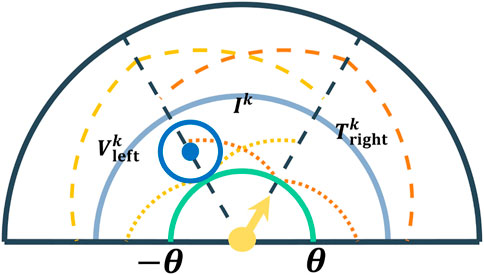
FIGURE 5. Description of Algorithm Part. The black dashed line denotes the partitioning of the environment, each of angle $\frac{2\theta }{3}$. The region between the orange (resp. yellow) dashed curve and the orange (resp. yellow) dot curve on the left (resp. right) side of the vehicle (resp. turret) denotes the V_left (resp. T_right).

We now describe the motion of the defenders. The objective is to move the defenders such that intruders from any two sets out of $V_{\mathrm{l}\mathrm{e}\mathrm{f}\mathrm{t}}^k$, $T_{\mathrm{r}\mathrm{i}\mathrm{g}\mathrm{h}\mathrm{t}}^k$, and I^k are captured. This requires assigning the defenders to the sets containing maximum number of intruders, which can be summarized into two cases.

Case 1: The set I^k contains maximum number of intruders, i.e., $|I^k|\ge V_{\mathrm{l}\mathrm{e}\mathrm{f}\mathrm{t}}^k$ and $|I^k|\ge T_{\mathrm{r}\mathrm{i}\mathrm{g}\mathrm{h}\mathrm{t}}^k$ hold at the start of epoch k. This means that one of the defenders must be assigned to the set I^k. By determining which set has more intruders out of $V_{\mathrm{l}\mathrm{e}\mathrm{f}\mathrm{t}}^k$ and $T_{\mathrm{r}\mathrm{i}\mathrm{g}\mathrm{h}\mathrm{t}}^k$, Algorithm Part performs an assignment of the sets to the defenders. Mathematically, if $|I^k|\ge |V_{\mathrm{l}\mathrm{e}\mathrm{f}\mathrm{t}}^k|$ and $|I^k|\ge |T_{\mathrm{r}\mathrm{i}\mathrm{g}\mathrm{h}\mathrm{t}}^k|$, then

• If $|V_{\mathrm{l}\mathrm{e}\mathrm{f}\mathrm{t}}^k|\ge |T_{\mathrm{r}\mathrm{i}\mathrm{g}\mathrm{h}\mathrm{t}}^k|$, then the vehicle is assigned the set $V_{\mathrm{l}\mathrm{e}\mathrm{f}\mathrm{t}}^k$ and the turret is assigned the set I^k.

• Otherwise, the vehicle is assigned the set I^k and the turret is assigned the set $T_{\mathrm{r}\mathrm{i}\mathrm{g}\mathrm{h}\mathrm{t}}^k$.

Case 2: $|V_{\mathrm{l}\mathrm{e}\mathrm{f}\mathrm{t}}^k|<|I^k|$ or $|T_{\mathrm{r}\mathrm{i}\mathrm{g}\mathrm{h}\mathrm{t}}^k|<|I^k|$ holds at the start of epoch k. This implies that at least one set out of $V_{\mathrm{l}\mathrm{e}\mathrm{f}\mathrm{t}}^k$ and $T_{\mathrm{r}\mathrm{i}\mathrm{g}\mathrm{h}\mathrm{t}}^k$ has the maximum number of intruders out of the three $V_{\mathrm{l}\mathrm{e}\mathrm{f}\mathrm{t}}^k,I^k$, and $T_{\mathrm{r}\mathrm{i}\mathrm{g}\mathrm{h}\mathrm{t}}^k$ sets. Then, the sets are assigned as follows:

• If $|V_{\mathrm{l}\mathrm{e}\mathrm{f}\mathrm{t}}^k|<|I^k|$, then the vehicle is assigned the set I^k. Otherwise, the vehicle is assigned the set $V_{\mathrm{l}\mathrm{e}\mathrm{f}\mathrm{t}}^k$.

• Similarly, if $|T_{\mathrm{r}\mathrm{i}\mathrm{g}\mathrm{h}\mathrm{t}}^k|<|I^k|$, then the turret is assigned the set I^k. Otherwise, the turret is assigned the set $T_{\mathrm{r}\mathrm{i}\mathrm{g}\mathrm{h}\mathrm{t}}^k$. Note that if the vehicle is already assigned set I^k then that means that $|I^k|\ge |V_{\mathrm{l}\mathrm{e}\mathrm{f}\mathrm{t}}^k|$ holds. Given the condition in Case 2, this implies that $|T_{\mathrm{r}\mathrm{i}\mathrm{g}\mathrm{h}\mathrm{t}}^k|<|I^k|$ holds and the turret is assigned $T_{\mathrm{r}\mathrm{i}\mathrm{g}\mathrm{h}\mathrm{t}}^k$. Thus, in Case 2, both defenders are never assigned the set I^k.

Once the sets are assigned, the vehicle turns as follows. If the set assigned to the vehicle is I^k, then the vehicle moves clockwise with unit speed in the direction perpendicular to its position vector until it reaches location $(z_v,\frac{\theta }{3})$. Upon reaching the location, the vehicle moves anti-clockwise with unit speed in the direction perpendicular to its position vector until it returns to location $(z_v,-\frac{\theta }{3})$. Otherwise (if the vehicle is assigned the set $V_{\mathrm{l}\mathrm{e}\mathrm{f}\mathrm{t}}^k$), the vehicle moves anti-clockwise with unit speed in the direction perpendicular to its position vector until it reaches location (z_v, − θ). Upon reaching that location, the vehicle moves clockwise with unit speed in the direction perpendicular to its position vector until it returns to location $(z_v,-\frac{\theta }{3})$.

Before we describe the motion of the turret, we determine its angular speed to ensure that the defenders start an epoch at the same time instant. As we require that the defenders take the same amount of time to return to their starting locations in an epoch, we require that $\frac{4\theta }{3\omega }=\frac{4\theta }{3}{z}_v\Rightarrow \omega =\frac{1}{z_v}$, which means that the angular speed of the turret must be at least $\frac{1}{z_v}$.

We now describe the turret’s motion in an epoch. Similar to the motion of the vehicle, if the set assigned to the turret is I^k, then the turret turns to angle $-\frac{\theta }{3}$ and then turns back to the initial heading angle $\frac{\theta }{3}$ with angular speed $\frac{1}{z_v}$. Otherwise, the turret turns to angle θ and then back to angle $\frac{\theta }{3}$ with angular speed $\frac{1}{z_v}$.

Analogous to Lemma 4.4, we have the following lemma which ensures that any intruder that was not considered for comparison at the start of epoch k is considered for comparison at the start of epoch (k + 1).

Lemma 4: Any intruder which lies beyond the sets $V_{\mathrm{l}\mathrm{e}\mathrm{f}\mathrm{t}}^k,V_{\mathrm{r}\mathrm{i}\mathrm{g}\mathrm{h}\mathrm{t}}^k,T_{\mathrm{r}\mathrm{i}\mathrm{g}\mathrm{h}\mathrm{t}}^k$, and $T_{\mathrm{l}\mathrm{e}\mathrm{f}\mathrm{t}}^k$ at the start of epoch k will be contained in the sets $V_{\mathrm{l}\mathrm{e}\mathrm{f}\mathrm{t}}^{k+1},V_{\mathrm{r}\mathrm{i}\mathrm{g}\mathrm{h}\mathrm{t}}^{k+1},T_{\mathrm{r}\mathrm{i}\mathrm{g}\mathrm{h}\mathrm{t}}^{k+1}$, and $T_{\mathrm{l}\mathrm{e}\mathrm{f}\mathrm{t}}^{k+1}$, respectively, at the start of epoch (k + 1) if

$v\le \min \left\{\frac{3\left(\min \left\{1,z_v+r_c\right\}-\rho \right)}{4\theta z_v},\frac{3\left(r_t-\rho \right)}{4\theta z_v}\right\}$

Proof. The proof is analogous to the proof of Lemma 4.4 and has been omitted for brevity.

Corollary 4.9: Any intruder that lies beyond the set I^k at time instant k_s will be contained in the set I^k+1 at the start of epoch (k + 1) if the conditions of Lemma 4.8 hold.

Proof. The proof directly follows from the fact that Lemma 4.8 holds for both the defenders and I^k represents the intersection of $V_{\mathrm{r}\mathrm{i}\mathrm{g}\mathrm{h}\mathrm{t}}^k$ and $T_{\mathrm{l}\mathrm{e}\mathrm{f}\mathrm{t}}^k$.

Theorem 4.10: Algorithm Part is 1.5-competitive for any problem instance $\mathcal{P}$ with $\omega \ge \frac{1}{z_v}$ that satisfies

$v\le \min \left\{\frac{3\left(\min \left\{1,z_v+r_c\right\}-\rho \right)}{4\theta z_v},\frac{3\left(r_t-\rho \right)}{4\theta z_v}\right\}$

Proof. Observe that from Lemma 4.8 and Corollary 4.9, every intruder is accounted for and no intruder that is not considered for comparison in a particular epoch is lost under the condition on v. Now, from the definition of Algorithm Part, the defenders are assigned two sets out of the total three in every epoch. Further, the assignment is carried out in a way that the sets with maximum number of intruders are assigned to the defenders in every epoch. Assuming that there exists an optimal offline algorithm that captures all intruders from all three sets then, from Definition 1, competitive ratio of Algorithm Part is at most $\frac{3}{2}$.

5 Numerical observations

We now provide numerical visualization of the bounds derived in this work and emphasize on the (v, ρ) and (ω, ρ) parameter regime. These plots allow the defenders to choose an appropriate online algorithm out of the four proposed, based on the values of the problem parameters.

5.1 (ω, ρ) Parameter regime

Figure 6 shows the (ω, ρ) parameter regime plot for fixed values of r_t, r_c, θ, and v and provides insights into the requirement of the angular speed ω for different values of the ρ. Note that the markers represent a lower bound on the angular speed of the turret.

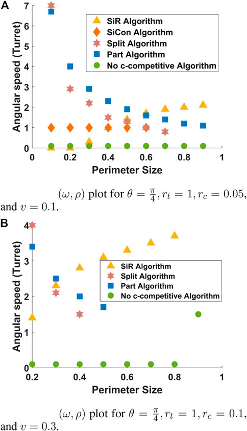
FIGURE 6

FIGURE 6. $(\omega ,\rho )$ plot for different values of $\theta ,r_c,r_t$, and $v$. Markers represent a lower bound on the turret's angular speed. (A) $(\omega ,\rho )$ plot for $\theta =\frac{\pi }{4},r_t=1,r_c=0.05$, and $v=0.1$. (B) $(\omega ,\rho )$ plot for $\theta =\frac{\pi }{4},r_t=1,r_c=0.1$, and $v=0.3$.

In Figure 6A, the condition in Theorem 3.1 for the existence of c-competitive algorithms is represented by the green circles. For all values of 0.1 ≤ ρ ≤ 0.9, as the green circles are at ω = 0.1, it implies that there exists a c-competitive algorithm for all values of ω ≥ 0.1 and the values of v, r_c, r_t, and θ selected for this figure. We now provide insights into the requirement on ω for our algorithms. Algorithm SiR, represented by the yellow triangle, requires higher angular speed for the turret as the radius of the perimeter increases. However, Algorithm Split and Algorithm Part, represented by the red star and blue square respectively, require lower angular speed for the turret when the radius of the perimeter is sufficiently large. Although counter intuitive, this can be explained as follows. Recall that Algorithm Part and Algorithm Split require the two defenders to be synchronous and the vehicle moves with a fixed unit speed. As the perimeter size increases, the time taken by the vehicle to complete its motion increases, which in turn requires lower values of ω to ensure synchronicity. Observe that for ρ ≥ 0.8, there are no markers for Algorithm Split. This is because for ρ ≥ 0.8 and the values of θ, r_t, r_c, and v considered for this figure, the condition defined for Algorithm Split in Theorem 4.6 is not satisfied for any 0 < ω ≤ 7, implying that Algorithm Split is not c-competitive. Analogous conclusions can be drawn for Algorithms SiCon (resp. Part), represented by orange diamond (resp. blue square), for values of ρ ≥ 0.6 (resp. ρ ≥ 0.9). Finally, note that Algorithm SiCon requires ω ≥ 1 for all values of ρ ≤ 0.6. This is because in this algorithm, the turret is required to move with unit angular speed to maintain synchronicity with the vehicle.

Analogous observations can be drawn in Figure 6B. For instance, when ρ = 0.9 and ω ≥ 1.5, there always exists a c-competitive algorithm with a finite constant c. Equivalently, there does not exist a c-competitive algorithm for ω < 1.5, ρ = 0.9 and for the values of r_t, r_c, θ, and v selected. Similarly, as ρ increases, Algorithm SiR requires a faster turret whereas Algorithm Part and Algorithm Split can work with a slower turret to ensure synchronicity. Note that Algorithm Part and Split do not have markers beyond ρ = 0.6 and ρ = 0.5, respectively, which is lower than the values of ρ in Figure 6A. This implies that, although the values of r_c are slightly higher than those in Figure 6A, it is more difficult to capture intruders given the higher value of v. Finally, there are no markers for Algorithm SiCon as it is not c-competitive for the values of parameters selected for this figure.

5.2 (v, ρ) Parameter regime

Figure 7 shows the (v, ρ) parameter regime for fixed values of θ, r_c, and r_t. Since, Algorithms Split, Part, SiCon require fixed but different values of ω, we set $\omega =\max \{\frac{1}{\min \{1,r_t+r_c\}},\frac{1}{z_v},\frac{\theta }{D}\}$. Note that the value of ω for this figure depends on the value of ρ as z_v is a function of ρ.

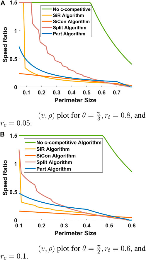
FIGURE 7

FIGURE 7. $(v,\rho )$ plot for different values of $\theta ,r_c$ and $r_t$. (A) $(v,\rho )$ plot for $\theta =\frac{\pi }{3},r_t=0.8$, and $r_c=0.05$. (B) $(v,\rho )$ plot for $\theta =\frac{\pi }{2},r_t=0.6$, and $r_c=0.1$.

Figure 7A shows the (v, ρ) parameter regime plot with θ, r_t, and r_c set to $\frac{\pi }{3},0.8$, and 0.05, respectively. For any value of parameters ρ and v, for instance 0.7 and 1, respectively, that lie beyond the green curve, there does not exists a c-competitive algorithm. For any value of parameters ρ and v that lie below the yellow curve, Algorithm SiR is 1-competitive. Similarly, for any value of parameters ρ and v that lie below the blue curve, Algorithm Part is 1.5-competitive. Analogous observations can be made for Algorithm Sicon and Algorithm Split. Note that for parameter regime that lies below the yellow curve, Algorithm Part is not effective as there exists Algorithm SiR with a better competitive ratio. For instance, for ρ = 0.2 and v = 0.2, it is better to use Algorithm SiR as it has a lower competitive ratio. Observe that for very high values of ρ, Algorithm SiCon is the most effective as it has the highest parameter regime curve. Finally, the light red curve of Algorithm Split is divided into regions where each region corresponds to a specific competitiveness. An important characteristic for Algorithm Split is that it can be used to determine the tradeoff between the competitiveness and the desired parameter regime for a specific problem instance.

Figure 7B shows the (v, ρ) parameter regime plot with θ, r_t, and r_c set to $\frac{\pi }{2},0.6$, and 0.1, respectively. Note that the green curve, which represents the curve for Theorem 3.1, is shifted slightly upwards as compared to in Figure 7A. This follows from the two cases considered in the proof which is based on the capture capability of the defenders (vehicle is now more capable and Theorem 3.1 is independent of r_t). As the angle of the environment increases and the engagement range of the turret decreases, it is harder to capture intruders. This is visualized in Figure 7B as the curves for all the algorithms have shifted downward compared to those in Figure 7A. Finally, for values of ρ > 0.3, Algorithm Part is more effective than Algorithm Split only if the competitive ratio of Algorithm Split is less than 1.5 for the chosen values of parameters. Similar to the curve of Algorithm Split, note that the curve for Algorithm SiR is also divided into regions. This is because of the different values of ω for different perimeter sizes.

6 Discussion

In this section, we provide a brief discussion on the time complexity of our algorithms and how this work extends to different models of the vehicle. We start with the time complexity of our algorithms.

6.1 Time complexity

We now establish the time complexity of each our algorithms and show that they can be implemented in real time if the information about the total number of intruders in every epoch is provided to the defenders.

Algorithm SiR and SiCon: Since Algorithm SiR and SiCon are open loop algorithms, the time complexity is O (1).

Algorithm Split: There are three quantities that must be computed at the start of every epoch of Algorithm Split, i.e., $|P_{\mathrm{r}\mathrm{i}\mathrm{g}\mathrm{h}\mathrm{t}}^k|,|P_{\mathrm{l}\mathrm{e}\mathrm{f}\mathrm{t}}^k|$, and $N_{p^{*}}$. Since $N_{p^{*}}$ is determined using a max() function over N sectors, its time complexity is O(N). Similarly, determining the sets $P_{\mathrm{r}\mathrm{i}\mathrm{g}\mathrm{h}\mathrm{t}}^k$ and $P_{\mathrm{l}\mathrm{e}\mathrm{f}\mathrm{t}}^k$ also have a time complexity of O(n), where n is the number of intruders in an epoch. This yields that the time complexity of Algorithm Split is O(max{n, N}). Recall that N is finite as r_c > 0. Thus, in the case when n → ∞, if the information about the number of intruders in $P_{\mathrm{r}\mathrm{i}\mathrm{g}\mathrm{h}\mathrm{t}}^k$ and $P_{\mathrm{l}\mathrm{e}\mathrm{f}\mathrm{t}}^k$ is provided to the defenders (through some external sensors), then this algorithm can be implemented in real time.

Algorithm Part: Similar to Algorithm Split, Algorithm Part computes $|T_{\mathrm{r}\mathrm{i}\mathrm{g}\mathrm{h}\mathrm{t}}^k|,|V_{\mathrm{l}\mathrm{e}\mathrm{f}\mathrm{t}}^k|$, and |I^k| at the start of every epoch which yields that the time complexity of Algorithm Part is O(n). This requires that the information about the total number of intruders in each of these sets must be provided to the defenders, for n → ∞, to implement this algorithm in real time.

6.2 Different motion models for the vehicle

We now discuss how this work extends to different motion model of the vehicle.

Observe that the analysis in this work is based upon two quantities; first, the time taken by the intruders to reach the perimeter and second, the time taken by the defenders to complete the motion. This work can be extended to other models for the vehicle, for instance double integrator, by suitably modifying the time taken by the vehicle to complete its motion. By doing so, it may be that the parameter regimes may be lower than in Figure 7 but the bounds on the competitive ratios will remain the same. The reason that the parameter regimes will be lower is as follows. Note that the parameter regimes are characterized by the conditions determined for each of the algorithms. Essentially, these conditions are determined by requiring the intruders to be sufficiently slow such that they take more time to reach the perimeter than the time taken by the vehicle to complete its motion. For a different model of the vehicle, such as the Dubins model, the path and the time taken by the vehicle to complete its motion can be determined by suitably incorporating the turn radius. Precise dependence of the competitiveness of such realistic models will be a topic of a future investigation.

7 Conclusions and future extensions

This work analyzed a perimeter defense problem in which two cooperative heterogeneous defenders, a mobile vehicle with finite capture range and a turret with finite engagement range, are tasked to defend a perimeter against mobile intruders that arrive in the environment. Our approach was based on a competitive analysis that first yielded a fundamental limit on the problem parameters for finite competitiveness of any online algorithm. We then designed and analyzed four algorithms and established sufficient conditions that guaranteed a finite competitive ratio for each algorithm under specific parameter regimes.

Apart from closing the gap between the curve that represents Theorem 3.1 and the curve that represents Algorithm Split, key future directions include multiple heterogeneous defender scenarios with energy constraints. Analyzing the problem with a weaker model of the adversary, realistic motion motions, maneuvering intruders, or with asymmetric information are also potential extensions.

Data availability statement

The original contributions presented in the study are included in the article/supplementary material, further inquiries can be directed to the corresponding author.

Author contributions

SB contributed towards the problem formulation, algorithm design, conceptual analysis, the results and preparing the manuscript. AVM contributed towards problem formulation and the literature review section. DWC contributed towards the problem formulation. SDB and ET contributed towards evaluating and improving the analysis and the presentation. All authors contributed equally towards reading and revising the manuscript and approving the submitted version.

Funding

This research was supported by the Aerospace Systems Technology Research and Assessment (ASTRA) Aerospace Technology Development and Testing (ATDT) program at AFRL under contract number FA865021D2602. Approved for public release: distribution unlimited, case number: AFRL-2022-6028.

Conflict of interest

The authors declare that the research was conducted in the absence of any commercial or financial relationships that could be construed as a potential conflict of interest.

Publisher’s note

All claims expressed in this article are solely those of the authors and do not necessarily represent those of their affiliated organizations, or those of the publisher, the editors and the reviewers. Any product that may be evaluated in this article, or claim that may be made by its manufacturer, is not guaranteed or endorsed by the publisher.

Footnotes

¹As the speed of the intruders is normalized by the speed of the vehicle, we use the speed of intruders and speed ratio interchangeably.

²The time taken by the defenders must be at most the time taken by the intruders to reach the perimeter.

³This case arises when the Algorithm Split moves the turret in the same direction for at least two consecutive epochs.

References

Adler, A., Mickelin, O., Ramachandran, R. K., Sukhatme, G. S., and Karaman, S. (2022). The role of heterogeneity in autonomous perimeter defense problems. arXiv preprint arXiv:2202.10433.

Google Scholar

Akilan, Z., and Fuchs, Z. (2017). “Zero-sum turret defense differential game with singular surfaces,” in 2017 IEEE conference on control Technology and applications (CCTA), 2041–2048. doi:10.1109/CCTA.2017.8062754

CrossRef Full Text | Google Scholar

Bajaj, S., and Bopardikar, S. D. (2019). “Dynamic boundary guarding against radially incoming targets,” in 2019 IEEE 58th conference on decision and control (CDC) (IEEE), 4804–4809.

CrossRef Full Text | Google Scholar

Bajaj, S., Bopardikar, S. D., Torng, E., Moll, A. V., and Casbeer, D. W. (2022). Competitive perimeter defense with multiple vehicles. In IEEE transactions on robotics. Under Review.

Google Scholar

Bajaj, S., Bopardikar, S. D., Von Moll, A., Torng, E., and Casbeer, D. W. (2022). “Perimeter defense using a turret with finite range and service times,” in 2023 American control conference (ACC) (IEEE).

Google Scholar

Bajaj, S., Torng, E., and Bopardikar, S. D. (2021). “Competitive perimeter defense on a line,” in 2021 American control conference (ACC) (IEEE), 3196–3201.

CrossRef Full Text | Google Scholar

Bajaj, S., Torng, E., Bopardikar, S. D., Von Moll, A., Weintraub, I., Garcia, E., et al. (2022). “Competitive perimeter defense of conical environments,” in 2022 IEEE 61st conference on decision and control (CDC) (IEEE), 6586–6593. doi:10.1109/CDC51059.2022.9993007

CrossRef Full Text | Google Scholar

Bertsimas, D. J., and Van Ryzin, G. (1991). A stochastic and dynamic vehicle routing problem in the Euclidean plane. Operations Res. 39, 601–615. doi:10.1287/opre.39.4.601

CrossRef Full Text | Google Scholar

Borodin, A., and El-Yaniv, R. (2005). Online computation and competitive analysis. Cambridge University Press.

Google Scholar

Bullo, F., Frazzoli, E., Pavone, M., Savla, K., and Smith, S. L. (2011). Dynamic vehicle routing for robotic systems. Proc. IEEE 99, 1482–1504. doi:10.1109/jproc.2011.2158181

CrossRef Full Text | Google Scholar

Casey, M. (2014). Drones bring fight and flight to battle against poachers. Sci. Am. (online) 20.

Google Scholar

Chen, M., Zhou, Z., and Tomlin, C. J. (2016). Multiplayer reach-avoid games via pairwise outcomes. IEEE Trans. Automatic Control 62, 1451–1457. doi:10.1109/tac.2016.2577619

CrossRef Full Text | Google Scholar

Deng, X., and Mirzaian, A. (1996). Competitive robot mapping with homogeneous markers. IEEE Trans. Robotics Automation 12, 532–542. doi:10.1109/70.508436

CrossRef Full Text | Google Scholar

Francos, R. M., and Bruckstein, A. M. (2021). Search for smart evaders with swarms of sweeping agents. IEEE Trans. Robotics 38, 1080–1100. doi:10.1109/tro.2021.3104253

CrossRef Full Text | Google Scholar

Garcia, E., Casbeer, D. W., Von Moll, A., and Pachter, M. (2020). Multiple pursuer multiple evader differential games. IEEE Trans. Automatic Control 66, 2345–2350. doi:10.1109/tac.2020.3003840

CrossRef Full Text | Google Scholar

Garcia, E., Von Moll, A., Casbeer, D. W., and Pachter, M. (2019). “Strategies for defending a coastline against multiple attackers,” in 2019 IEEE 58th conference on decision and control (CDC) (IEEE), 7319–7324.

CrossRef Full Text | Google Scholar

Guerrero-Bonilla, L., Nieto-Granda, C., and Egerstedt, M. (2021). “Robust perimeter defense using control barrier functions,” in 2021 international symposium on multi-robot and multi-agent Systems (MRS) (IEEE), 164–172.

CrossRef Full Text | Google Scholar

Howard, A., Parker, L. E., and Sukhatme, G. S. (2006). Experiments with a large heterogeneous mobile robot team: Exploration, mapping, deployment and detection. Int. J. Robotics Res. 25, 431–447. doi:10.1177/0278364906065378

CrossRef Full Text | Google Scholar

Isaacs, R. (1999). Differential games: A mathematical theory with applications to warfare and pursuit, control and optimization. Courier Corporation.

Google Scholar

Kappel, K. S., Cabreira, T. M., Marins, J. L., de Brisolara, L. B., and Ferreira, P. R. (2020). Strategies for patrolling missions with multiple UAVs. J. Intelligent Robotic Syst. 99, 499–515. doi:10.1007/s10846-019-01090-2

CrossRef Full Text | Google Scholar

Koveos, Y., Panousopoulou, A., Kolyvas, E., Reppa, V., Koutroumpas, K., Tsoukalas, A., et al. (2007). “An integrated power aware system for robotic-based lunar exploration,” in 2007 IEEE/RSJ international conference on intelligent robots and Systems (IEEE), 827–832.

CrossRef Full Text | Google Scholar

Lee, E. S., Shishika, D., and Kumar, V. (2020). “Perimeter-defense game between aerial defender and ground intruder,” in 2020 59th IEEE conference on decision and control (CDC) (IEEE), 1530–1536.

CrossRef Full Text | Google Scholar

Lee, Y., and Bakolas, E. (2021). “Optimal strategies for guarding a compact and convex target set: A differential game approach,” in 2021 60th IEEE conference on decision and control (CDC) (IEEE), 4320–4325.

CrossRef Full Text | Google Scholar

Lykou, G., Moustakas, D., and Gritzalis, D. (2020). Defending airports from uas: A survey on cyber-attacks and counter-drone sensing technologies. Sensors 20, 3537. doi:10.3390/s20123537

PubMed Abstract | CrossRef Full Text | Google Scholar

Macharet, D. G., Chen, A. K., Shishika, D., Pappas, G. J., and Kumar, V. (2020). “Adaptive partitioning for coordinated multi-agent perimeter defense,” in 2020 IEEE/RSJ international conference on intelligent robots and Systems (IROS) (IEEE), 7971–7977.

CrossRef Full Text | Google Scholar

Margellos, K., and Lygeros, J. (2011). Hamilton–Jacobi formulation for reach–avoid differential games. IEEE Trans. automatic control 56, 1849–1861. doi:10.1109/tac.2011.2105730

CrossRef Full Text | Google Scholar

Ma’sum, M. A., Arrofi, M. K., Jati, G., Arifin, F., Kurniawan, M. N., Mursanto, P., et al. (2013). “Simulation of intelligent unmanned aerial vehicle (UAV) for military surveillance,” in 2013 international conference on advanced computer science and information Systems (ICACSIS), 161–166. doi:10.1109/ICACSIS.2013.6761569

CrossRef Full Text | Google Scholar

McGee, T. G., and Hedrick, J. K. (2006). “Guaranteed strategies to search for mobile evaders in the plane,” in 2006 American control conference (IEEE), 2819–2824.

CrossRef Full Text | Google Scholar

Ozsoyeller, D., Beveridge, A., and Isler, V. (2013). Symmetric rendezvous search on the line with an unknown initial distance. IEEE Trans. Robotics 29, 1366–1379. doi:10.1109/tro.2013.2272252

CrossRef Full Text | Google Scholar

Psaraftis, H. N. (1988). Dynamic vehicle routing problems. Veh. routing Methods Stud. 16, 223–248.

Google Scholar

Ramachandran, R. K., Pierpaoli, P., Egerstedt, M., and Sukhatme, G. S. (2021). Resilient monitoring in heterogeneous multi-robot systems through network reconfiguration. IEEE Trans. Robotics 38, 126–138. doi:10.1109/tro.2021.3128313

CrossRef Full Text | Google Scholar

Ramachandran, R. K., Preiss, J. A., and Sukhatme, G. S. (2019). “Resilience by reconfiguration: Exploiting heterogeneity in robot teams,” in 2019 IEEE/RSJ international conference on intelligent robots and Systems (IROS) (IEEE), 6518–6525.

CrossRef Full Text | Google Scholar

Sabag, O., Lale, S., and Hassibi, B. (2022). “Competitive-ratio and regret-optimal control with general weights,” in 2022 IEEE 61st conference on decision and control (CDC) (IEEE), 4859–4864. doi:10.1109/CDC51059.2022.9993106

CrossRef Full Text | Google Scholar

Santos, M., and Egerstedt, M. (2018). “Coverage control for multi-robot teams with heterogeneous sensing capabilities using limited communications,” in 2018 IEEE/RSJ international conference on intelligent robots and Systems (IROS) (IEEE), 5313–5319.

CrossRef Full Text | Google Scholar

Shishika, D., and Kumar, V. (2020). “A review of multi agent perimeter defense games,” in International conference on decision and game theory for security (Springer), 472–485.

CrossRef Full Text | Google Scholar

Sleator, D. D., and Tarjan, R. E. (1985). Amortized efficiency of list update and paging rules. Commun. ACM 28, 202–208. doi:10.1145/2786.2793

CrossRef Full Text | Google Scholar

Smith, S. L., Bopardikar, S. D., and Bullo, F. (2009). “A dynamic boundary guarding problem with translating targets,” in Decision and control, 2009 held jointly with the 2009 28th Chinese control conference. CDC/CCC 2009 (IEEE), 8543–8548.

CrossRef Full Text | Google Scholar

Tavakoli, M., Cabrita, G., Faria, R., Marques, L., and de Almeida, A. T. (2012). Cooperative multi-agent mapping of three-dimensional structures for pipeline inspection applications. Int. J. Robotics Res. 31, 1489–1503. doi:10.1177/0278364912461536

CrossRef Full Text | Google Scholar

Von Moll, A., and Fuchs, Z. E. (2020). “Optimal constrained retreat within the turret defense differential game,” in 2020 IEEE conference on control Technology and applications (CCTA) (IEEE), 611–618.

CrossRef Full Text | Google Scholar

Von Moll, A., and Fuchs, Z. (2021). “Turret lock-on in an engage or retreat game,” in American Control Conference. IEEE, 3188–3195. doi:10.23919/ACC50511.2021.9483106

CrossRef Full Text | Google Scholar

Von Moll, A., Pachter, M., Shishika, D., and Fuchs, Z. (2022). Circular target defense differential games. Trans. Automatic Control 68. doi:10.1109/TAC.2022.3203357

CrossRef Full Text | Google Scholar

Von Moll, A., Shishika, D., Fuchs, Z., and Dorothy, M. (2022). Turret–runner–penetrator differential game with role selection. Trans. Aerosp. Electron. Syst. 58, 5687–5702. doi:10.1109/TAES.2022.3176599

CrossRef Full Text | Google Scholar

Yan, R., Shi, Z., and Zhong, Y. (2018). Reach-avoid games with two defenders and one attacker: An analytical approach. IEEE Trans. Cybern. 49, 1035–1046. doi:10.1109/tcyb.2018.2794769

PubMed Abstract | CrossRef Full Text | Google Scholar

Yan, R., Shi, Z., and Zhong, Y. (2019). Task assignment for multiplayer reach–avoid games in convex domains via analytical barriers. IEEE Trans. Robotics 36, 107–124. doi:10.1109/tro.2019.2935345

CrossRef Full Text | Google Scholar