Obstacle-avoidance trajectory planning and sliding mode-based tracking control of an omnidirectional mobile robot

1 Introduction

With the development of science and technology, mobile robots are more and more widely implemented in industry and services industries and services. For simple and repetitive transportation tasks in factories and warehouses, it is more efficient and economical to utilize mobile robots instead of labor force (Kassaeiyan et al., 2019; Mai et al., 2019; Zou, 2019; Wang et al., 2021). In addition, on some dangerous occasions, robots are more suitable than humans to complete the corresponding hazardous tasks. Compared with traditional mobile robots, an omnidirectional mobile robot possesses high mobility and good maneuverability due to transient movement in any direction without a swerve (Clavien et al., 2018). Therefore, this type of mobile robot has attracted extensive attention from academia and industry. In order to achieve omnidirectional mobility, researchers and engineers have designed omnidirectional mobile robots with various structures, such as a spherical mobile robot (Chen et al., 2013), a roller mobile robot (Terakawa et al., 2018), and a snake-like mobile robot (Fukushima et al., 2012). Among all kinds of omnidirectional mobile robots, the Mecanum-wheeled omnidirectional mobile robot (MWOMR) is a classical type. A typical Mecanum wheel is equipped with a series of rotary rollers at the edge of the wheel hub evenly, and the rollers’ axles are normally set to form an angle of 45° with the Mecanum wheel’s axle (Cooney et al., 2004). When a Mecanum wheel rotates, the roller that touches the ground will generate friction along the roller’s axle. Hence, through the combination of the rotational movements of all Mecanum wheels installed on an MWOMR, a resultant force can be generated in an arbitrarily predetermined direction, which can thereby realize the omnidirectional-movement characteristics.

Trajectory planning and tracking control are key technologies to realize the autonomous movement of a mobile robot. The meaning of trajectory planning is to generate a series of reference position-and-posture signals for a mobile robot according to the surrounding-environment information perceived by the robot, while the kinematic constraints of the robot and its surrounding obstacles are taken into consideration. Based on the need for environmental information, trajectory planning can be classified into global planning and local planning. A global planning algorithm not only takes a long time to be executed but also needs all environmental information a priori, which results in the difficulty of actual implementations. Compared with global planning, local planning possesses a stronger real-time property by utilizing the environmental information collected by sensors to iteratively update the reference trajectory. Typical local planning strategies mainly include fuzzy logic methods (Chen et al., 2022), artificial potential field (APF)-based methods (Tian et al., 2021), neural network methods (Zhang et al., 2017), etc., among these methods, the APF scheme utilizes a virtual resultant force generated by the target and obstacles to guide the movement of a mobile robot (Huang et al., 2020). Due to the advantages of smooth-trajectory generation and real-time obstacle-avoidance ability, APF-based strategies play a key role in trajectory planning for mobile robots.

In addition to trajectory planning, motion control is also a hot research topic in the field of mobile robots. Among various control strategies, sliding mode control has been widely utilized in numerous kinds of mechatronic engineering practices owing to its superior performance and firm robustness in handling external disturbances and model uncertainties (Zong et al., 2013; Li et al., 2018; Nguyen et al., 2018; Alipour et al., 2019; Sun et al., 2019; Saha et al., 2022). Elementary Conventional sliding mode control is only able to realize asymptotic convergence. To overcome this shortage, a terminal sliding mode control method is developed to enhance the convergence speed and suppress the chattering phenomenon (Man et al., 1995). On this basis, a non-singular terminal sliding mode control method is further proposed to address the singularity problem that exists in classical terminal sliding mode control (Feng et al., 2002). The non-singular terminal sliding mode control has a wide spectrum of applications, such as the control of a vehicle steer-by-wire system (Sun et al., 2017) and a servomotor rigid robot (Ba et al., 2019).

With the improvement of the computational capabilities of embedded control apparatuses, more and more control algorithms are implemented by computer control systems. Normally, computer control systems require sampling periods, which means that the control input signal remains constant during a sampling period (Young et al., 1999). For sliding mode control, discrete control inputs can bring the system states close to the sliding surface, but usually cannot make the states stay on the sliding surface (Yu et al., 2012). Direct application of a continuous sliding mode control algorithm to a discrete-time system may harm the stability of the system and even result in a loss of control. In order to deploy effective control schemes on sampled-data systems, discrete sliding mode control is investigated and developed. In (Gao et al., 1995), the concepts of quasi-sliding mode and quasi-sliding mode bands are elaborated, and an approaching condition for discrete single-input-single-output systems is established. In (Wu and Sun, 2015), a discrete chattering-free repetitive sliding mode control method is proposed and applied to a motor system. Aiming at the problem of a large switching gain of sliding mode control when dealing with external disturbances, an extended state observer-based feedforward-compensation sliding mode control strategy is presented (Ma et al., 2022). In (Hou and Wang, 2019), combining a discrete-time predictor with sliding mode control, a model-free sliding mode control method is developed such that the control system possesses strong robustness against large non-linear hysteresis.

Considering the unique merits of APF-based methods and sliding mode control, we combine these two powerful tools, propose an APF-based trajectory-planning scheme and a discrete integral terminal sliding mode (DITSM)-based trajectory-tracking control scheme for an MWOMR such that the robot can plan and follow an obstacle-avoidance trajectory, and finally arrive at a predetermined target. The contributions of this paper can be summarised as follows:

1) Based on the kinematic-and-dynamic mechanism analysis, a discrete-time plant model is identified to describe the MWOMR’s movement characteristics, which lays the foundation of subsequent trajectory planning and tracking control.

2) An APF-based trajectory-planning method is proposed for the MWOMR via the position information of the robot, obstacles, and target. Furthermore, the planned reference trajectory can be calculated and updated iteratively such that the scenario of dynamic obstacles can also be handled well.

3) An effective DITSM control algorithm is designed for the MWOMR, which cooperates with the trajectory-planning method well and guarantees that the robot can track the planned trajectory accurately. In addition, the control system possesses firm robustness against system uncertainties and disturbances.

The rest of this paper is organized as follows: In Section 2, a continuous kinematic-and-dynamic model is established for the MWOMR, and it is properly discretized by the Euler method. In Section 3, an APF-based trajectory-planning algorithm and a DITSM-based trajectory-tracking control algorithm are designed for the MWOMR. The stability of the control system is analyzed and assured via the Lyapunov stability criterion. In Section 4, simulation results in the scenarios of static obstacles and dynamic obstacles are illustrated and analyzed, which verifies the effectiveness and superiority of the proposed strategy. Last, the conclusion of this paper is given in Section 5.

2 Modeling

For the issue of trajectory planning and tracking control of an MWOMR, the identification of a precise model based on the analysis in kinematics and dynamics plays a fundamental role. To facilitate the corresponding analysis, a vertical-view schematic is introduced here as shown in Figure 1. In this schematic, there exists a global coordinate frame Y_gO_gX_g and a rotational coordinate frame Y_rO_rX_r sharing the same origin O_g (O_r). Note that the coordinate frame Y_rO_rX_r rotates with the MWOMR simultaneously, which implies that ω_r = ω_g as shown in Figure 1. Then, we utilize the parameter $P_g={[x_g,y_g,{\omega }_g]}^T$ to describe the MWOMR’s position and heading under the global coordinate. The component [x_g, y_g] denotes the robot’s displacements along the X_g and Y_g axes, respectively; the parameter ω_g is the robot’s yaw angle around its center of gravity O_CG. Likewise, the parameter $P_r={[x_r,y_r,{\omega }_r]}^T$ is employed to describe the robot’s position and posture under the rotational coordinate.

FIGURE 1

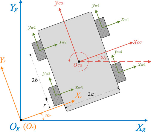
FIGURE 1. Vertical-view schematic of MWOMR.

According to the kinematics illustrated in Figure 1, it can be inferred that

${\dot{P}}_g=\left[\begin{array}{c}\hfill {\dot{x}}_g\hfill \\ \hfill {\dot{y}}_g\hfill \\ \hfill {\dot{\omega }}_g\hfill \end{array}\right]=T_r\left({\omega }_g\right){\dot{P}}_r=T_r\left({\omega }_g\right)\left[\begin{array}{c}\hfill {\dot{x}}_r\hfill \\ \hfill {\dot{y}}_r\hfill \\ \hfill {\dot{\omega }}_r\hfill \end{array}\right](1)$

where T_r (ω_g) is a transformation matrix between the two coordinate frames, and its expression is given by

$T_r\left({\omega }_g\right)=\left[\begin{array}{ccc}\hfill \cos \left({\omega }_g\right)\hfill & \hfill -\sin \left({\omega }_g\right)\hfill & \hfill 0\hfill \\ \hfill \sin \left({\omega }_g\right)\hfill & \hfill \cos \left({\omega }_g\right)\hfill & \hfill 0\hfill \\ \hfill 0\hfill & \hfill 0\hfill & \hfill 1\hfill \end{array}\right].(2)$

According to Sun et al. (2021), we have the following kinematic relationship between the derivative of P_r and the Mecanum wheels’ angular velocities:

${\dot{P}}_r=\left[\begin{array}{c}\hfill {\dot{x}}_r\hfill \\ \hfill {\dot{y}}_r\hfill \\ \hfill {\dot{\omega }}_r\hfill \end{array}\right]=\frac{r}{4}\left[\begin{array}{cccc}\hfill -1\hfill & \hfill 1\hfill & \hfill -1\hfill & \hfill 1\hfill \\ \hfill 1\hfill & \hfill 1\hfill & \hfill 1\hfill & \hfill 1\hfill \\ \hfill \frac{1}{a+b}\hfill & \hfill -\frac{1}{a+b}\hfill & \hfill -\frac{1}{a+b}\hfill & \hfill \frac{1}{a+b}\hfill \end{array}\right]\cdot \left[\begin{array}{c}\hfill {\dot{\theta }}_1\hfill \\ \hfill {\dot{\theta }}_2\hfill \\ \hfill {\dot{\theta }}_3\hfill \\ \hfill {\dot{\theta }}_4\hfill \end{array}\right](3)$

where 2a and 2b represent the main body width of the MWOMR and the distance between the front and rear Mecanum-wheel axles as shown in Figure 1, respectively; r denotes the radius of all Mecanum wheels since their dimensions are identical; θ_i is the rotation angle of the i^th Mecanum wheel.

Combining (Eqs. 1–3) yields

${\dot{P}}_g=\left[\begin{array}{c}\hfill {\dot{x}}_g\hfill \\ \hfill {\dot{y}}_g\hfill \\ \hfill {\dot{\omega }}_g\hfill \end{array}\right]=\frac{r}{4}h\left(\omega \right)\dot{\theta }(4)$

where $\theta ={[{\theta }_1,{\theta }_2,{\theta }_3,{\theta }_4]}^T$, and h(ω) is a matrix with the following expression:

$h\left(\omega \right)=\sqrt{2}\left[\begin{array}{cccc}\hfill -\sin \left(\omega \right)\hfill & \hfill \cos \left(\omega \right)\hfill & \hfill -\sin \left(\omega \right)\hfill & \hfill \cos \left(\omega \right)\hfill \\ \hfill \cos \left(\omega \right)\hfill & \hfill \sin \left(\omega \right)\hfill & \hfill \cos \left(\omega \right)\hfill & \hfill \sin \left(\omega \right)\hfill \\ \hfill \frac{1}{\sqrt{2}\left(a+b\right)}\hfill & \hfill -\frac{1}{\sqrt{2}\left(a+b\right)}\hfill & \hfill -\frac{1}{\sqrt{2}\left(a+b\right)}\hfill & \hfill \frac{1}{\sqrt{2}\left(a+b\right)}\hfill \end{array}\right](5)$

with $\omega ={\omega }_g+\frac{\pi }{4}$. Then, according to Eq. 4, we can get the second-order derivative of P_g as:

${\ddot{P}}_g=\frac{r}{4}h{\left(\omega \right)}^{\prime }\dot{\theta }+\frac{r}{4}h\left(\omega \right)\ddot{\theta }(6)$

where

$h{\left(\omega \right)}^{\prime }=\sqrt{2}\left[\begin{array}{cccc}\hfill -\cos \left(\omega \right)\dot{\omega }\hfill & \hfill -\sin \left(\omega \right)\dot{\omega }\hfill & \hfill -\cos \left(\omega \right)\dot{\omega }\hfill & \hfill -\sin \left(\omega \right)\dot{\omega }\hfill \\ \hfill -\sin \left(\omega \right)\dot{\omega }\hfill & \hfill \cos \left(\omega \right)\dot{\omega }\hfill & \hfill -\sin \left(\omega \right)\dot{\omega }\hfill & \hfill \cos \left(\omega \right)\dot{\omega }\hfill \\ \hfill 0\hfill & \hfill 0\hfill & \hfill 0\hfill & \hfill 0\hfill \end{array}\right].(7)$

As shown in Figure 1, there exist four Mecanum wheels in the WMOMR, and they are connected with four motors installed on the robot body such that the motors can generate appropriate torques to drive the corresponding Mecanum wheels. Based on the mechanism analysis, the dynamic model of the wheel-and-motor system can be identified as:

$J_0\ddot{\theta }+b_0\dot{\theta }+d=u(8)$

where J₀ and b₀ stand for the nominal moment of inertia and viscous friction of each motor-connected wheel, respectively; $d={[d_1,d_2,d_3,d_4]}^T$ denotes the lumped system uncertainties; $u={[u_1,u_2,u_3,u_4]}^T$ is the control input, i.e., the output torques of the corresponding motors. Note that all the Mecanum wheels possess the same dimension and material. Thus, the parameters J₀ and b₀ are unified for all wheels. Furthermore, according to the robot’s mechanical and dynamic characteristics, it can be assumed that the uncertainty components d_i are bounded and satisfy the following condition:

$|d_i|<\bar{d}(9)$

where the parameter d $\bar{d}$ denotes the corresponding upper bound presumed to be known a priori.

Combining the kinematic model as shown in Eq. 6 and the wheel-and-motor dynamic model given by Eq. 8, the following plant model can be obtained:

${\ddot{P}}_g=\frac{r}{4J_0}h\left(\omega \right)\left(H\dot{\omega }\dot{\theta }-b_0\dot{\theta }-d+u\right)(10)$

where H is a matrix whose expression is as follows:

$H=\left[\begin{array}{cccc}\hfill 0\hfill & \hfill \frac{J_0}{2}\hfill & \hfill 0\hfill & \hfill \frac{J_0}{2}\hfill \\ \hfill -\frac{J_0}{2}\hfill & \hfill 0\hfill & \hfill -\frac{J_0}{2}\hfill & \hfill 0\hfill \\ \hfill 0\hfill & \hfill \frac{J_0}{2}\hfill & \hfill 0\hfill & \hfill \frac{J_0}{2}\hfill \\ \hfill -\frac{J_0}{2}\hfill & \hfill 0\hfill & \hfill -\frac{J_0}{2}\hfill & \hfill 0\hfill \end{array}\right].(11)$

Finally, for the convenience of realizing the obstacle-avoidance trajectory planning and tracking control simultaneously, it is necessary to discretize the above continuous-time plant model. A corresponding discrete-time model is obtained as follows:

$\begin{array}{cc}\hfill \mathrm{\Delta }{P}_g\left(k\right)& =v\left(k\right)\hfill \\ \hfill \mathrm{\Delta }v\left(k\right)& =\frac{r}{4J_0}h\left(\omega \left(k\right)\right)\left[H{v}_{\omega g}\left(k\right)\psi \left(k\right)-b_0\psi \left(k\right)+u\left(k\right)-d\left(k\right)\right]\hfill \end{array}(12)$

where the parameter $\psi (k)={[{\psi }_1(k),{\psi }_2(k),{\psi }_3(k),{\psi }_4(k)]}^T$ denotes the wheel angular velocity. $v(k)={[v_{xg}(k),v_{yg}(k),v_{\omega g}(k)]}^T$ represents the MWOMR’s velocities in terms of horizontal displacement, vertical displacement, and heading direction, respectively. By employing the Euler discretization method, we have:

$\begin{array}{cc}\hfill \mathrm{\Delta }{P}_g\left(k\right)& =\frac{P_g\left(k+1\right)-P_g\left(k\right)}{T}\hfill \\ \hfill \mathrm{\Delta }v\left(k\right)& =\frac{v\left(k+1\right)-v\left(k\right)}{T}\hfill \end{array}(13)$

where T stands for the sampling period in the discretization procedure. Up to now, the plant model to be utilized in the subsequent obstacle-avoidance trajectory planning and tracking control has been established.

3 Trajectory planning and tracking control

3.1 Obstacle-avoidance trajectory planning

For an APF-based trajectory-planning method, the target and obstacles are regarded as objects that exert virtual attractive and repulsive forces on the robot, respectively. The resultant force indicates the MWOMR’s moving direction, and it guides the robot to bypass obstacles and arrive at the target.

According to (Tian et al., 2021), an attractive-field function can be set as:

$U_{att}\left(k\right)=\left\{\begin{array}{cc}\frac{1}{2}\zeta l^2\left(k\right)\hfill & l\left(k\right)\le l^{*}\hfill \\ l^{*}\zeta l\left(k\right)-\frac{1}{2}\zeta {\left(l^{*}\right)}^2\hfill & l\left(k\right)>l^{*}\hfill \end{array}\right.(14)$

where l(k) represents the distance between the robot and target at the sampling moment of k; ζ is an attractive-field parameter; l* is a switching distance positive constant that denotes a distance threshold of the function. Then, we can get an attractive force which is the first-order derivative of the corresponding attractive-field function:

$\nabla U_{\mathit{att}}\left(k\right)=\left\{\begin{array}{cc}\zeta l\left(k\right)\hfill & l\left(k\right)\le l^{*}\hfill \\ l^{*}\zeta \hfill & l\left(k\right)>l^{*}.\hfill \end{array}\right.(15)$

The purpose of setting the attractive-field function as a piecewise function as shown in Eq. 14 is to avoid an overlarge attractive force if the robot is far away from the target. Otherwise, if the attractive force is always proportional to the distance l(k), the robot will be forced to rush at a high velocity from the starting point. With the setting of Eq. 14, a constant attractive force will be generated and exerted on the robot until the robot enters an area with a predetermined radius l* around the destination.

On the other hand, we set a repulsive-field function as:

$U_{\mathit{rep}}^i\left(k\right)=\left\{\begin{array}{cc}\frac{1}{2}\kappa {\left(\frac{1}{L^i\left(k\right)}-\frac{1}{Q^{*}}\right)}^2\hfill & L^i\left(k\right)\le Q^{*}\hfill \\ 0,\hfill & L^i\left(k\right)>Q^{*}\hfill \end{array}\right.(16)$

where κ represents the repulsive-field coefficient; Lⁱ(k) denotes the distance between the i^th obstacle and the mobile robot; Q* stands for the maximum acting range of the repulsive field. Similar to the attractive force, the corresponding repulsive force can be obtained as follows:

$\nabla U_{rep}^i\left(k\right)=\left\{\begin{array}{cc}-\kappa \left(\frac{1}{L^i\left(k\right)}-\frac{1}{Q^{*}}\right)\frac{1}{{\left(L^i\left(k\right)\right)}^2}\hfill & L^i\left(k\right)\le Q^{*}\hfill \\ 0\hfill & L^i\left(k\right)>Q^{*}.\hfill \end{array}\right.(17)$

According to the above analysis, the resultant force acting on the robot is:

$F\left(k\right)=\nabla U_{att}\left(k\right)-\sum _{i=1}^N\nabla U_{rep}^i\left(k\right).(18)$

The resultant force is composed of two components in the directions of the X and Y-axes. Then, the reference velocities of the robot are generated in the directions of the X and Y-axes, which can be used as the reference signal of the trajectory-tracking control system.

3.2 Trajectory-tracking controller design

In this section, a DITSM control algorithm is designed for the MWOMR. According to the dynamic model as shown in Eq. 12, the velocity error is defined as:

$\begin{array}{c}\hfill e_v\left(k\right)=\left[\begin{array}{c}\hfill e_{v1}\left(k\right)\hfill \\ \hfill e_{v2}\left(k\right)\hfill \\ \hfill e_{v3}\left(k\right)\hfill \end{array}\right]=\left[\begin{array}{c}\hfill v_{xg}\left(k\right)-v_{xd}\left(k\right)\hfill \\ \hfill v_{yg}\left(k\right)-v_{yd}\left(k\right)\hfill \\ \hfill v_{\omega g}\left(k\right)-v_{\omega d}\left(k\right)\hfill \end{array}\right]\end{array}(19)$

where $v_d(k)={\left[v_{xd}(k),v_{yd}(k),v_{\omega d}(k)\right]}^T$ denotes the reference velocity signal of the control system. Then, we can construct a DITSM surface (Yu et al., 2012) as follows:

$\begin{array}{c}\hfill s\left(k\right)=\left[\begin{array}{c}\hfill s_1\left(k\right)\hfill \\ \hfill s_2\left(k\right)\hfill \\ \hfill s_3\left(k\right)\hfill \end{array}\right]=\left[\begin{array}{c}\hfill e_{v1}\left(k\right)+\beta E_1\left(k-1\right)\hfill \\ \hfill e_{v2}\left(k\right)+\beta E_2\left(k-1\right)\hfill \\ \hfill e_{v3}\left(k\right)+\beta E_3\left(k-1\right)\hfill \end{array}\right].\end{array}(20)$

In Eq. 20, the integral term E (k − 1) is with the following expression:

$\begin{array}{c}\hfill E\left(k-1\right)=\left[\begin{array}{c}\hfill {\sum }_{i=0}^{k-1}{e}_{v1}^{p/q}\left(i\right)\hfill \\ \hfill {\sum }_{i=0}^{k-1}{e}_{v2}^{p/q}\left(i\right)\hfill \\ \hfill {\sum }_{i=0}^{k-1}{e}_{v3}^{p/q}\left(i\right)\hfill \end{array}\right]=\left[\begin{array}{c}\hfill E_1\left(k-2\right)+e_{v1}^{p/q}\left(k-1\right)\hfill \\ \hfill E_2\left(k-2\right)+e_{v2}^{p/q}\left(k-1\right)\hfill \\ \hfill E_3\left(k-2\right)+e_{v3}^{p/q}\left(k-1\right)\hfill \end{array}\right]\end{array}(21)$

where the parameters p, q > 0 are odd integers and satisfy $0<\frac{q}{p}<1$; β > 0 is another control parameter to be tuned.

Based on the concept of equivalent control input as described in (Slotine and Li, 1991), we temporarily assume that the lumped parametric uncertainties are zero, i.e., d(k) = [0, 0, 0, 0]^T, and substitute (20) into s (k + 1) − s(k) = 0, then we get:

$\begin{array}{c}\hfill e_v\left(k+1\right)+\beta E\left(k\right)-s\left(k\right)=0.\end{array}(22)$

Combining Eqs, 13, 19, 22, we can get:

$\begin{array}{c}\hfill v_g\left(k\right)+T\mathrm{\Delta }{v}_g\left(k\right)-v_d\left(k+1\right)+\beta E\left(k\right)-s\left(k\right)=0.\end{array}(23)$

Substituting (Eqs. 12, 23) yields the equivalent control input u_eq as:

$\begin{array}{c}\hfill u_{eq}\left(k\right)=\frac{4J_0}{rT}h{\left(\omega \left(k\right)\right)}^{†}\left[v_d\left(k+1\right)-v_g\left(k\right)+s\left(k\right)-\beta E\left(k\right)\right]-H{v}_{\omega g}\left(k\right)\psi \left(k\right)+b_0\psi \left(k\right)\end{array}(24)$

where

${h\left(\omega \left(k\right)\right)}^{†}=\frac{1}{4}\left[\begin{array}{ccc}\hfill -\sqrt{2}\sin \left(\omega \left(k\right)\right)\hfill & \hfill \sqrt{2}\cos \left(\omega \left(k\right)\right)\hfill & \hfill a+b\hfill \\ \hfill \sqrt{2}\cos \left(\omega \left(k\right)\right)\hfill & \hfill \sqrt{2}\sin \left(\omega \left(k\right)\right)\hfill & \hfill -\left(a+b\right)\hfill \\ \hfill -\sqrt{2}\sin \left(\omega \left(k\right)\right)\hfill & \hfill \sqrt{2}\cos \left(\omega \left(k\right)\right)\hfill & \hfill -\left(a+b\right)\hfill \\ \hfill \sqrt{2}\cos \left(\omega \left(k\right)\right)\hfill & \hfill \sqrt{2}\sin \left(\omega \left(k\right)\right)\hfill & \hfill a+b\hfill \end{array}\right](25)$

and it satisfies h (ω(k))h (ω(k))^† = I_{3 × 3}. Note that the so-called equivalent control input is derived from s (k + 1) − s(k) = 0 while temporarily neglecting the system uncertainties. Hence, the expression of u_eq as shown in Eq. 24 does not contain the lumped uncertainties d. The system uncertainties can be handled by a reaching control input which will be designed subsequently.

In order to ensure the robustness of the control system, a reaching control input u_r is designed as:

$\begin{array}{c}\hfill u_r\left(k\right)=-\frac{4J_0}{r}h{\left(\omega \left(k\right)\right)}^{†}K\mathrm{s}\mathrm{g}\mathrm{n}\left(s\left(k\right)\right)\end{array}(26)$

where $K=\text{diag}(2\epsilon ,2\epsilon ,\frac{2\epsilon }{a+b})$, and ɛ is a control parameter to be selected. Where K is the switching gain of the designed reaching control input. For the convenience of the subsequent stability analysis of the control system, K is defined as

$\begin{array}{c}\hfill K=\text{diag}\left(2\epsilon ,2\epsilon ,\frac{2\epsilon }{a+b}\right)\end{array}(27)$

where the parameter ɛ should be chosen to satisfy the following condition:

$\begin{array}{c}\hfill \epsilon >\frac{r}{J_0}\bar{d}.\end{array}(28)$

Note that the main reason for the above setting as shown in Eqs. 27, 28 is to assure that the control system is stable and the corresponding stability analysis procedure can be simplified to a large extent. Another reason is that this setting can also reduce the difficulty of tuning the switching gain K, since only one parameter ɛ needs to be selected.

Lemma 1. For the MWOMR system as described in Eq. 12, the control input is designed as

$\begin{array}{c}\hfill u\left(k\right)=u_{eq}\left(k\right)+u_r\left(k\right)\end{array}(29)$

where u_eq(k) and u_r(k) are given by (Eqs. 24, 26), respectively. Meanwhile, the switching gainɛ is chosen to satisfy the condition of$\epsilon >\frac{r}{J_0}\bar{d}$Then, the following convergence property can be guaranteed:

1) The discrete sliding variable s(k) can converge into a bounded region Ω in finite steps with the following expression:

$\begin{array}{cc}\hfill \mathrm{\Omega }& =\left\{s\left(k\right)||s_i\left(k\right)|<{\epsilon }_{si}\right\}\hfill \\ \hfill {\epsilon }_s& =\left[\begin{array}{c}\hfill {\epsilon }_{s1}\hfill \\ \hfill {\epsilon }_{s2}\hfill \\ \hfill {\epsilon }_{s3}\hfill \end{array}\right]=\left[\begin{array}{c}\hfill 4T\epsilon -\frac{rT}{J_0}\bar{d}\hfill \\ \hfill 4T\epsilon -\frac{rT}{J_0}\bar{d}\hfill \\ \hfill \frac{4T}{a+b}\epsilon -\frac{rT}{J_0\left(a+b\right)}\bar{d}\hfill \end{array}\right].\hfill \end{array}(30)$

2) Once the sliding variable converges into Ω, it will stay within this region and cannot escape. In other words, if s(k) ∈ Ω, then s (k + 1) ∈ Ω.

3) The tracking error e_v(k) can converge into a bounded region as follows:

$\begin{array}{cc}\hfill |e_{v1}\left(k\right)|& \le \psi \left(\sigma \right)\cdot \max \left\{{\left(\frac{4\bar{d}}{\beta }\right)}^{1/\sigma },{\beta }^{\frac{1}{1-\sigma }}\right\}\hfill \\ \hfill |e_{v2}\left(k\right)|& \le \psi \left(\sigma \right)\cdot \max \left\{{\left(\frac{4\bar{d}}{\beta }\right)}^{1/\sigma },{\beta }^{\frac{1}{1-\sigma }}\right\}\hfill \\ \hfill |e_{v3}\left(k\right)|& \le \psi \left(\sigma \right)\cdot \max \left\{{\left(\frac{4\bar{d}}{\beta \left(a+b\right)}\right)}^{1/\sigma },{\beta }^{\frac{1}{1-\sigma }}\right\}\hfill \end{array}(31)$

where $\sigma =\frac{q}{p}$, and $\psi (\sigma )=1+{\sigma }^{\frac{\sigma }{1-\sigma }}-{\sigma }^{\frac{1}{1-\sigma }}$.To demonstrate the structure of the proposed strategy more intuitively, a block diagram is shown in Figure 2.

FIGURE 2

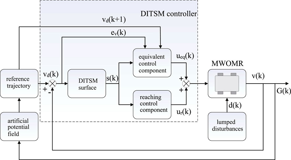
FIGURE 2. Block diagram of proposed strategy.

3.3 Stability proof

To confirm the stability of the whole control system, we set a discrete-time Lyapunov function as:

$V\left(k\right)=s{\left(k\right)}^{T}s\left(k\right).(32)$

According to the definition of the Lyapunov function V(k), the following equation can be obtained:

$\begin{array}{cc}\hfill V\left(k+1\right)-V\left(k\right)& =s{\left(k+1\right)}^{T}s\left(k+1\right)-s{\left(k\right)}^{T}s\left(k\right)\hfill \\ \hfill & =s_1^2\left(k+1\right)+s_2^2\left(k+1\right)+s_3^2\left(k+1\right)-s_1^2\left(k\right)-s_2^2\left(k\right)-s_3^2\left(k\right)\hfill \\ \hfill & =\left[s_1\left(k+1\right)-s_1\left(k\right)\right]\left[s_1\left(k+1\right)+s_1\left(k\right)\right]\left[s_2\left(k+1\right)+s_2\left(k\right)\right]\left[s_2\left(k+1\right)-s_2\left(k\right)\right]+\left[s_3\left(k+1\right)-s_3\left(k\right)\right]\left[s_3\left(k+1\right)+s_3\left(k\right)\right].\hfill \end{array}(33)$

Combining (Eqs. 12, 20, 29), we can get the expression of s (k + 1) as:

$\begin{array}{c}\hfill s\left(k+1\right)=\left[\begin{array}{c}\hfill s_1\left(k\right)-2T\epsilon \mathrm{sgn}\left(s_1\left(k\right)\right)+\frac{rT}{4J_0}{D}_1\left(k\right)\hfill \\ \hfill \hfill \\ \hfill s_2\left(k\right)-2T\epsilon \mathrm{sgn}\left(s_2\left(k\right)\right)+\frac{rT}{4J_0}{D}_2\left(k\right)\hfill \\ \hfill \hfill \\ \hfill s_3\left(k\right)-\frac{2T}{a+b}\epsilon \mathrm{sgn}\left(s_3\left(k\right)\right)+\frac{rT}{4J_0}{D}_3\left(k\right)\hfill \end{array}\right]\end{array}(34)$

where the expressions of D₁, D₂, and D₃ are given by:

$\begin{array}{cc}\hfill D_1\left(k\right)& =\sqrt{2}\left[\sin \left(\omega \left(k\right)\right)d_1\left(k\right)-\cos \left(\omega \left(k\right)\right)d_2\left(k\right)+\sin \left(\omega \left(k\right)\right)d_3\left(k\right)-\cos \left(\omega \left(k\right)\right)d_4\left(k\right)\right]\hfill \\ \hfill & \le 4\bar{d}\hfill \\ \hfill D_2\left(k\right)& =\sqrt{2}\left[-\cos \left(\omega \left(k\right)\right)d_1\left(k\right)-\sin \left(\omega \left(k\right)\right)d_2\left(k\right)-\cos \left(\omega \left(k\right)\right)d_3\left(k\right)-\sin \left(\omega \left(k\right)\right)d_4\left(k\right)\right]\hfill \\ \hfill & \le 4\bar{d}\hfill \\ \hfill D_3\left(k\right)& =-\frac{1}{a+b}{d}_1\left(k\right)+\frac{1}{a+b}{d}_2\left(k\right)+\frac{1}{a+b}{d}_3\left(k\right)-\frac{1}{a+b}{d}_4\left(k\right)\hfill \\ \hfill & \le \frac{4}{a+b}\bar{d}.\hfill \end{array}(35)$

Afterward, a classified discussion is carried out to prove that the sliding variable s can converge into the region Ω.

3.3.1 The situation of s_i(k) > ɛ_si

According to Eqs. 20, 34, we can obtain

$\begin{array}{cc}\hfill s_1\left(k+1\right)-s_1\left(k\right)& =-2T\epsilon \mathrm{sgn}\left(s_1\left(k\right)\right)+\frac{rT}{4J_0}{D}_1\left(k\right)\hfill \\ \hfill & <-2T\epsilon +\frac{rT}{J_0}\bar{d}\hfill \\ \hfill & <-T\epsilon \hfill \end{array}(36)$

and

$\begin{array}{cc}\hfill s_1\left(k+1\right)+s_1\left(k\right)& =2s_1\left(k\right)-2T\epsilon +\frac{rT}{4J_0}{D}_1\left(k\right)\hfill \\ \hfill & >2{\epsilon }_{s1}-2T\epsilon +\frac{rT}{4J_0}{D}_1\left(k\right)\hfill \\ \hfill & =8T\epsilon -2\frac{rT}{J_0}\bar{d}-2T\epsilon +\frac{rT}{4J_0}{D}_1\left(k\right)\hfill \\ \hfill & >T\epsilon +\left(5T\epsilon -2\frac{rT}{J_0}\bar{d}-\frac{rT}{J_0}\bar{d}\right)\hfill \\ \hfill & >T\epsilon .\hfill \end{array}(37)$

Thus, from (Eqs. 36, 37), we can easily infer that

$s_1^2\left(k+1\right)-s_1^2\left(k\right)<-T^2{\epsilon }^2.(38)$

Since s₁(k) and s₂(k) as shown in Eq. 30 possess the same convergence area, the deducing steps to prove that s₂(k) converges into Ω are similar to the above analysis. Thus, it can be inferred that

$s_2^2\left(k+1\right)-s_2^2\left(k\right)<-T^2{\epsilon }^2.(39)$

Next, we analyze the situation of s₃(k) > ɛ_s3. Following the above steps, we can get:

$\begin{array}{cc}\hfill s_3\left(k+1\right)-s_3\left(k\right)& =-\frac{2T}{a+b}\epsilon \mathrm{sgn}\left(s_3\left(k\right)\right)+\frac{rT}{4J_0}{D}_3\left(k\right)\hfill \\ \hfill & <-\frac{2T}{a+b}\epsilon +\frac{rT}{J_0\left(a+b\right)}\bar{d}\hfill \\ \hfill & <-\frac{T}{a+b}\epsilon \hfill \end{array}(40)$

and

$\begin{array}{cc}\hfill s_3\left(k+1\right)+s_3\left(k\right)& =2s_3\left(k\right)-\frac{2T}{a+b}\epsilon \mathrm{sgn}\left(s_3\left(k\right)\right)+\frac{rT}{4J_0}{D}_3\left(k\right)\hfill \\ \hfill & >2{\epsilon }_{s3}-\frac{2T}{a+b}\epsilon \mathrm{sgn}\left(s_3\left(k\right)\right)+\frac{rT}{4J_0}{D}_3\left(k\right)\hfill \\ \hfill & =\frac{8T}{a+b}\epsilon -2\frac{rT}{J_0\left(a+b\right)}\bar{d}-\frac{2T}{a+b}\epsilon +\frac{rT}{4J_0}{D}_3\left(k\right)\hfill \\ \hfill & >\frac{T}{a+b}\epsilon +\left[\frac{5T}{a+b}\epsilon -2\frac{rT}{J_0\left(a+b\right)}\bar{d}-\frac{rT}{J_0}\bar{d}\right]\hfill \\ \hfill & >\frac{T}{a+b}\epsilon .\hfill \end{array}(41)$

According to (Eqs. 40, 41), it can be deduced that $s_3^2(k+1)-s_3^2(k)<-\frac{T^2{\epsilon }^2}{{(a+b)}^2}$.

3.3.2 The situation of s_i(k) < −ɛ_si

The theoretical analysis in this situation can also be carried out by utilizing similar deducing steps as shown in (Eqs. 36–41).

In summary, when |s_i(k)| > ɛ_si, we have the following conclusion:

$\begin{array}{c}\hfill \left\{\begin{array}{c}{s}_1^2\left(k+1\right)-s_1^2\left(k\right)<-T^2{\epsilon }^2\hfill \\ s_2^2\left(k+1\right)-s_2^2\left(k\right)<-T^2{\epsilon }^2\hfill \\ s_3^2\left(k+1\right)-s_3^2\left(k\right)<-\frac{T^2{\epsilon }^2}{{\left(a+b\right)}^2}.\hfill \end{array}\right.\end{array}(42)$

Furthermore, the above formula can be extended as follows:

$\begin{array}{cc}\hfill & s_1^2\left(\eta \right)<s_1^2\left(0\right)-\eta T^2{\epsilon }^2<{\epsilon }_{s1}^2\hfill \\ \hfill & s_2^2\left(\eta \right)<s_2^2\left(0\right)-\eta T^2{\epsilon }^2<{\epsilon }_{s2}^2\hfill \\ \hfill & s_3^2\left(\eta \right)<s_3^2\left(0\right)-\frac{\eta T^2{\epsilon }^2}{{\left(a+b\right)}^2}<{\epsilon }_{s3}^2\hfill \end{array}(43)$

which means that when s (0) is outside the region Ω, the sliding variable s can converge into this region within η steps. The expression of η is given by:

$\eta =\mathrm{m}\mathrm{a}\mathrm{x}\left\{\frac{s_1^2\left(0\right)-{\epsilon }_{s1}^2}{T^2{\epsilon }^2}+1,\frac{s_2^2\left(0\right)-{\epsilon }_{s2}^2}{T^2{\epsilon }^2}+1,\frac{{\left(a+b\right)}^2\left[s_3^2\left(0\right)-{\epsilon }_{s3}^2\right]}{T^2{\epsilon }^2}+1\right\}.(44)$

Remark 1. During the converging procedure, the convergence of s₁, s₂, and s₃ is independent. Hence, the parameter η is the number of steps for the last one of s_i to converge into the region Ω.Up to now, we have proved that the sliding variable s(k) can converge into the region Ω. Next, we need to analyze whether s (k + 1) can remain within this region or not.First, considering the range of 0 < s_i (k) < ɛ_si, we can get:

$\begin{array}{cc}\hfill s_1\left(k+1\right)& =s_1\left(k\right)-2T\epsilon +\frac{rT}{4J_0}{D}_1\left(k\right)\hfill \\ \hfill & <{\epsilon }_{s1}-2T\epsilon +\frac{rT}{4J_0}{D}_1\left(k\right)\hfill \\ \hfill & <{\epsilon }_{s1}-2T\epsilon +\frac{rT}{J_0}\bar{d}\hfill \\ \hfill & <{\epsilon }_{s1}\hfill \end{array}(45)$

and

$\begin{array}{cc}\hfill s_1\left(k+1\right)& =s_1\left(k\right)-2T\epsilon +\frac{rT}{4J_0}{D}_1\left(k\right)\hfill \\ \hfill & >-4T\epsilon +\frac{rT}{J_0}\bar{d}+\left[4T\epsilon -2T\epsilon +\frac{rT}{4J_0}{D}_1\left(k\right)-\frac{rT}{J_0}\bar{d}\right]\hfill \\ \hfill & >-{\epsilon }_{s1}.\hfill \end{array}(46)$

From Eqs. 45, 46, we can see that when 0 < s₁k) < ɛ_s1, s₁ (k + 1) will remain in the region of |s₁ (k + 1)| ≤ ɛ_s1.For the situation of 0 < s₂ (k + 1) < ɛ_s2, we have:

$\begin{array}{cc}\hfill s_2\left(k+1\right)& =s_2\left(k\right)-2T\epsilon +\frac{rT}{4J_0}{D}_2\left(k\right)\hfill \\ \hfill & <{\epsilon }_{s2}-2T\epsilon +\frac{rT}{4J_0}{D}_2\left(k\right)\hfill \\ \hfill & <{\epsilon }_{s2}-2T\epsilon +\frac{rT}{J_0}\bar{d}\hfill \\ \hfill & <{\epsilon }_{s2}\hfill \end{array}(47)$

and

$\begin{array}{cc}\hfill s_2\left(k+1\right)& =s_2\left(k\right)-2T\epsilon +\frac{rT}{4J_0}{D}_2\left(k\right)\hfill \\ \hfill & >-4T\epsilon +\frac{rT}{J_0}\bar{d}+\left[4T\epsilon -2T\epsilon +\frac{rT}{4J_0}{D}_2\left(k\right)-\frac{rT}{J_0}\bar{d}\right]\hfill \\ \hfill & >-{\epsilon }_{s2}.\hfill \end{array}(48)$

Thus, when 0 < s₂k) < ɛ_s2, it can be inferred that |s₂ (k + 1)| ≤ ɛ_s2.For the situation of 0 < s₃ (k + 1) < ɛ_s3, we can get:

$\begin{array}{cc}\hfill s_3\left(k+1\right)& =s_3\left(k\right)-\frac{2T}{a+b}\epsilon +\frac{rT}{4J_0}{D}_3\left(k\right)\hfill \\ \hfill & <{\epsilon }_{s3}-\frac{T}{a+b}\epsilon \hfill \\ \hfill & <{\epsilon }_{s3}\hfill \end{array}(49)$

and

$\begin{array}{cc}\hfill s_3\left(k+1\right)& =s_3\left(k\right)-\frac{2T}{a+b}\epsilon +\frac{rT}{4J_0}{D}_3\left(k\right)\hfill \\ \hfill & >-\frac{4T}{a+b}\epsilon +\frac{rT}{J_0\left(a+b\right)}\bar{d}+\left[\frac{4T}{a+b}\epsilon -\frac{2T}{a+b}\epsilon -\frac{rT}{J_0\left(a+b\right)}\bar{d}+\frac{rT}{4J_0}{D}_3\left(k\right)\right]\hfill \\ \hfill & >-{\epsilon }_{s3}.\hfill \end{array}(50)$

Hence, when 0 < s₃k) < ɛ_s3, we can infer that |s₃ (k + 1)| ≤ ɛ_s3.Similar to the analysis procedure as shown in 45–50, for the range of −ɛ_si < s_i(k) < 0, we can also derive the conclusion of |s_i (k + 1)| ≤ ɛ_si.Thus, we have completed the proof of s (k + 1) ∈ Ω. In other words, under the action of the proposed DITSM control law, the sliding variable s can converge into the region Ω in finite steps without escaping from this region.

Lemma 2. (Li et al., 2014): Considering the dynamics of a discrete-time terminal sliding surface e (k + 1) = e(k) − le(k)^σ + g(k) with |g(k)| ≤ γ, the variable e(k) can converge into a bounded region in finite steps shown as follows:

$|e\left(k\right)|\le \psi \left(\sigma \right)\cdot \max \left\{{\left(\frac{\gamma }{l}\right)}^{1/\sigma },l^{\frac{1}{1-\sigma }}\right\}(51)$

where the function ψ(σ) is defined as

$\psi \left(\sigma \right)=1+{\sigma }^{\frac{\sigma }{1-\sigma }}-{\sigma }^{\frac{1}{1-\sigma }}.(52)$

It has been proved that the proposed DITSM control law can drive the sliding variable s into the region Ω. Based on the definition of the DITSM surface, we have:

$\begin{array}{c}\hfill \left[\begin{array}{c}\hfill e_{v1}\left(k+1\right)\hfill \\ \hfill e_{v2}\left(k+1\right)\hfill \\ \hfill e_{v3}\left(k+1\right)\hfill \end{array}\right]=\left[\begin{array}{c}\hfill e_{v1}\left(k\right)-\beta e_{v1}^{p/q}\left(k\right)+\frac{rT}{4J_0}{D}_1\left(k\right)\hfill \\ \hfill e_{v2}\left(k\right)-\beta e_{v2}^{p/q}\left(k\right)+\frac{rT}{4J_0}{D}_2\left(k\right)\hfill \\ \hfill e_{v3}\left(k\right)-\beta e_{v3}^{p/q}\left(k\right)+\frac{rT}{4J_0}{D}_3\left(k\right)\hfill \end{array}\right].\end{array}(53)$

Finally, according to the conclusion given by Lemma 2, we can infer that:

$\begin{array}{cc}\hfill |e_{v1}\left(k\right)|& \le \psi \left(\sigma \right)\cdot \max \left\{{\left(\frac{4\bar{d}}{\beta }\right)}^{1/\sigma },{\beta }^{\frac{1}{1-\sigma }}\right\}\hfill \\ \hfill |e_{v2}\left(k\right)|& \le \psi \left(\sigma \right)\cdot \max \left\{{\left(\frac{4\bar{d}}{\beta }\right)}^{1/\sigma },{\beta }^{\frac{1}{1-\sigma }}\right\}\hfill \\ \hfill |e_{v3}\left(k\right)|& \le \psi \left(\sigma \right)\cdot \max \left\{{\left(\frac{4\bar{d}}{\beta \left(a+b\right)}\right)}^{1/\sigma },{\beta }^{\frac{1}{1-\sigma }}\right\}\hfill \end{array}(54)$

where $\sigma =\frac{q}{p}$. Then, it has been verified that the tracking error e_v(k) converges into a bounded region after finite steps.Thus, the stability proof of the control system is accomplished.

3.4 Selection of control parameters

3.4.1 Selection of p and q

The parameters p and q should be chosen as odd numbers and satisfy $0<\frac{q}{p}<1$. Note that the closer the value of $\frac{q}{p}$ gets to 1, the closer s is to a proportional sliding surface. Then, the control input signal is more smooth, but the convergence rate is slower. Considering this tradeoff, we set p = 5 and q = 3.

3.4.2 Selection of β

Increasing β can accelerate the convergence rate and keep small steady-state errors. However, an overlarge β may cause system instability. To strike a balance, we set β = 1.5.

3.4.3 Selection of ɛ

The parameter ɛ affects the convergence rate of tracking errors. A larger ɛ can accelerate the convergence procedure but at the cost of intensifying chattering. Weighing these two factors, we set ɛ = 8.

3.5 Benchmark controllers

For the aim of reflecting the advantages of the designed DITSM control algorithm, a discrete conventional sliding mode (DCSM) controller and a discrete terminal sliding mode (DTSM) controller are designed as benchmarks according to (Liu, 2005) and (Li et al., 2014), respectively. To save the paper layout, the stability proof of the benchmark control systems is omitted here, and the corresponding control inputs are given straightforwardly.

3.5.1 DCSM controler

The DCSM control input is designed as follows:

$\begin{array}{cc}\hfill u_c\left(k\right)=& \frac{4J_0}{rT}{h}^{-1}\left(\omega \left(k\right)\right)\left[v_d\left(k+1\right)-v_g\left(k\right)+s_c\left(k\right)-KT\mathrm{sgn}\left(s_c\left(k\right)\right)\right]\hfill \\ \hfill & -H{v}_{\omega g}\left(k\right)\psi \left(k\right)+b_0\psi \left(k\right)\hfill \end{array}(55)$

where s_c(k) is a traditional discrete sliding variable with the following definition:

$\begin{array}{c}\hfill s_c\left(k\right)=e_v\left(k\right).\end{array}(56)$

3.5.2 DTSM controler

Design the DTSM control input as:

$\begin{array}{cc}\hfill u_t\left(k\right)=& \frac{4J_0}{rT}{h}^{-1}\left(\omega \left(k\right)\right)\times \left[v_d\left(k+1\right)-v_g\left(k\right)+s_t\left(k\right)-\beta e_v^{p/q}\left(k\right)-KT\mathrm{sgn}\left(s_t\left(k\right)\right)\right]\hfill \\ \hfill & -H{v}_{\omega g}\left(k\right)\psi \left(k\right)+b_0\psi \left(k\right)\hfill \end{array}(57)$

where s_t(k) is a discrete terminal sliding variable defined as:

$\begin{array}{c}\hfill s_t\left(k\right)=e_v\left(k\right)+\beta e_v^{p/q}\left(k-1\right).\end{array}(58)$

4 Simulation results

To verify the effectiveness of the proposed trajectory-planning-and-tracking-control scheme, simulations via the software of MATLAB are carried out in two scenarios of static-obstacle avoidance and dynamic-obstacle avoidance.

Case 1. Static obstacles.In this case, the MWOMR is controlled to bypass static obstacles and reach the target. The initial positions of the robot and target are set as (0 m, 0 m) and (15 m, 0 m), respectively. Meanwhile, five static obstacles are set with the positions of (2 m, −0.75 m) (3 m, 1.2 m), (7 m, −0.1 m) (10 m, 1.5 m), and (13 m, 0.5 m). By utilizing the APF-based trajectory-planning method as shown in Eqs. 14–18, we set the attractive-field coefficient as ζ = 0.5, the repulsive-field coefficient as κ = 8, the switching coefficient as l* = 5, and the maximum acting range of the repulsive field as Q* = 3, respectively. To mimic the protection of the MWOMR’s motors, the motor output torque is limited to 0–15 Nm. The sampling period is set as T = 0.01s. Considering the computation load and operational efficiency, the trajectory-planning algorithm is set to be updated every 20 sampling periods. Meanwhile, to reflect the omnidirectional-movement characteristics of the MWOMR, the predetermined heading angle is set as zero, which means that the robot’s orientation always remains in the original state during the movement.The simulation results in Case 1 are shown in Figures 3–5. Figure 3 shows the obstacle-avoidance trajectories of the MWOMR under the action of three control strategies. The MWOMR’s X-axis velocity errors, Y-axis velocity errors, and heading-angle velocity errors are shown in Figure 4. As shown in Figure 4A, the DITSM controller possesses the fastest convergence rate in the X-axis velocity error, while the DTSM and DCSM controllers rank the second and the slowest, respectively. From Figure 4B we can see that there exist oscillations in the Y-axis velocity errors, which is mainly because the designed trajectory-planning algorithm updates every 20 sampling periods. However, it is evident that the oscillation amplitude under the action of the DITSM controller is the smallest, where the peak value is only 0.05 m/s. The motor output torques of all control systems are displayed in Figure 5. We can see that the initial action of the DITSM control system is the strongest, which leads to its fast convergence rate.

FIGURE 3

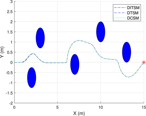
FIGURE 3. Obstacle-avoidance trajectories in Case 1.

FIGURE 4

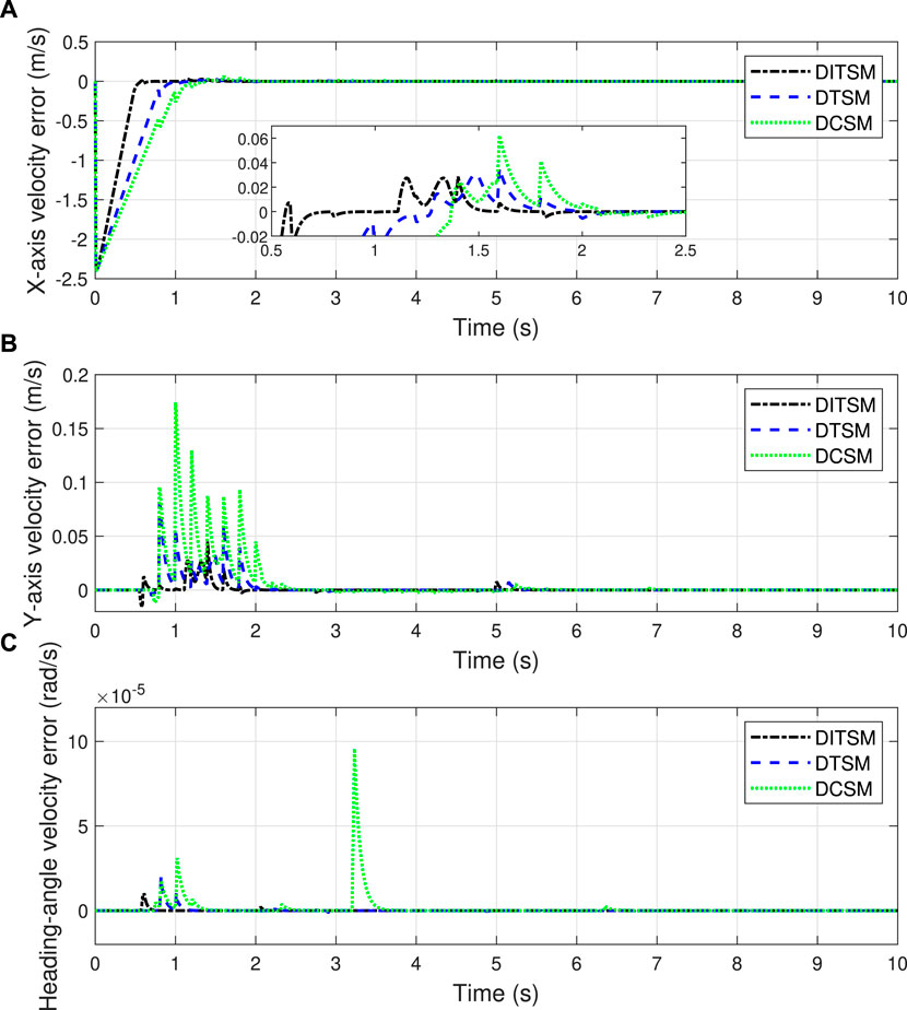
FIGURE 4. Velocity errors in Case 1. (A) X-axis velocity errors, (B) Y-axis velocity errors, (C) Orientation-angle velocity errors.

FIGURE 5

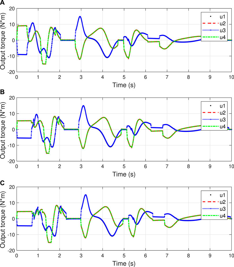
FIGURE 5. Control inputs in Case 1. (A) DITSM, (B) DTSM, (C) DCSM.

Case 2. Dynamic obstacles.Up to now, the performance of the proposed method has been verified in the scenario of static obstacles. However, for numerous actual scenarios, the obstacles are normally not static but dynamic. Hence, it is of great necessity to substantiate the effectiveness of the presented method when there exist moving obstacles. In this case, we set the initial positions of the 3rd and 4th obstacles as (7 m, −1 m) and (10 m, 1.5 m), respectively. In addition, the 3rd obstacle is set to move along the Y-axis at a velocity of 1 m/s within the range of [−1 m, 1 m], and the 4^th obstacle is set to move along the Y-axis at a velocity of 0.5 m/s within the range of [0 m, 3 m]. The other settings are kept the same as those of Case 1. The serial numbers of five obstacles and the dynamic-obstacle-avoidance screenshots are shown in Figure 6.Figures 6A–I shows the screenshots of the MWOMR’s moving trajectories with an interval of 0.5 s. We can see that the presented APF-based trajectory-planning scheme can update the reference trajectory according to the 3rd and 4th obstacles’ moving situations and guide the robot to bypass obstacles. The robot can realize a satisfactory dynamic-obstacle-avoidance performance under the action of the designed DITSM control law. Figures 7, 8 show the MWOMR’s whole moving trajectories, X-axis velocity errors, Y-axis velocity errors, and heading-angle velocity errors, respectively. It is evident that the DITSM control system possesses the fastest velocity-error convergence rate, the fastest transient response rate, and the smallest velocity-error oscillation amplitudes compared with those of the other controllers. The motor output torques are shown in Figure 9, from which it can be seen that the proposed DITSM control strategy can provide a larger control input at the initial moment and accordingly accelerate the convergence of tracking errors.From Case 1 and Case 2 we can see that the proposed APF-based trajectory-planning scheme can realize effective obstacle-avoidance trajectory planning in both static and dynamic scenarios. Meanwhile, compared with the DCSM and DTSM controllers, the presented DITSM control law possesses superior control performance in terms of higher tracking accuracy and firmer robustness in handling different scenarios.

FIGURE 6

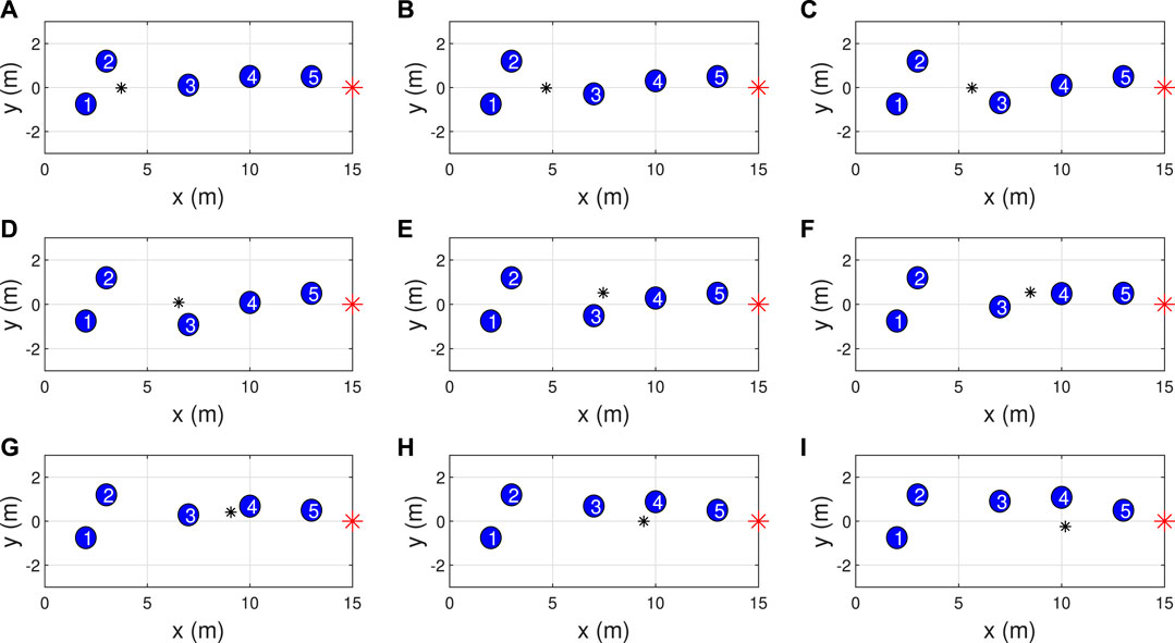
FIGURE 6. Dynamic obstacle avoidance of DITSM controller.

FIGURE 7

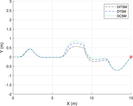
FIGURE 7. Obstacle-avoidance trajectories in Case 2.

FIGURE 8

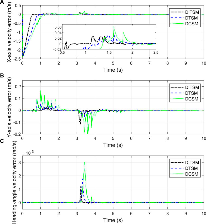
FIGURE 8. Velocity errors in Case 2. (A) X-axis velocity errors, (B) Y-axis velocity errors, (C) Orientation-angle velocity errors.

FIGURE 9

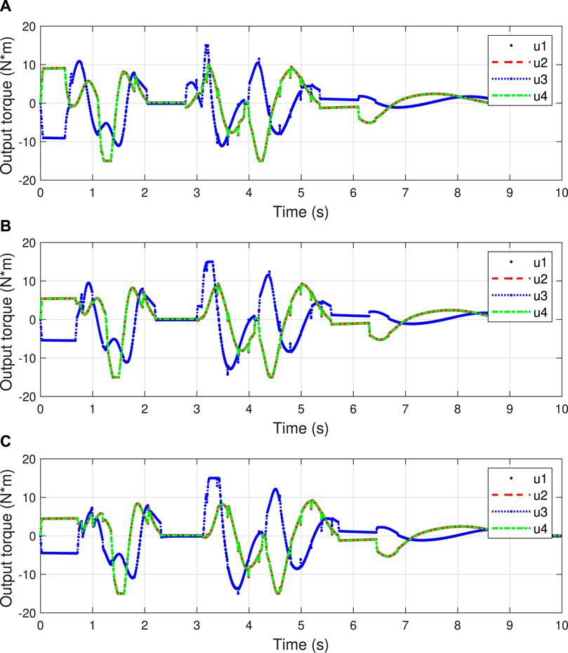
FIGURE 9. Control inputs in Case 2. (A) DITSM, (B) DTSM, (C) DCSM.

5 Conclusion

In this paper, we investigate the issue of obstacle-avoidance trajectory planning and tracking control of a Mecanum-wheeled omnidirectional mobile robot. A discrete kinematic-and-dynamic model is identified for the mobile robot. Then, an artificial potential field-based trajectory-planning algorithm is designed to guide the robot to bypass obstacles, and a discrete integral terminal sliding mode control strategy is proposed to force the robot to track the planned trajectory effectively. The stability of the control system is substantiated via the Lyapunov stability theory, and a tuning guideline of control parameters is elaborated in detail. Lastly, simulations in static-obstacle and dynamic-obstacle scenarios are accomplished for performance tests. The testing results indicate that the proposed trajectory-planning-and-tracking-control method can realize a satisfactory obstacle-avoidance performance for the omnidirectional mobile robot. In addition, compared with the benchmark controllers, the designed discrete integral terminal sliding mode control law demonstrates evident effectiveness and superiority.

Data availability statement

The original contributions presented in the study are included in the article/supplementary material, further inquiries can be directed to the corresponding author.

Author contributions

ZS: Manuscript writing and polishing; SH: Method design; XM: Simulations; BC: Resources; JZ: Manuscript revision; ZM: Control method suggestions; TW: Revision suggestions.

Funding

The authors would like to thank the National Natural Science Foundation of China (62003305), the Natural Science Foundation of Zhejiang Province (LQ21F030015), and the Key Research and Development Program of Zhejiang Province (2022C03029) for their support in this research.

Conflict of interest

Author TW was employed by the company Hangzhou RoboCT Technology Development Co. Ltd.

The remaining authors declare that the research was conducted in the absence of any commercial or financial relationships that could be construed as a potential conflict of interest.

Publisher’s note

All claims expressed in this article are solely those of the authors and do not necessarily represent those of their affiliated organizations, or those of the publisher, the editors and the reviewers. Any product that may be evaluated in this article, or claim that may be made by its manufacturer, is not guaranteed or endorsed by the publisher.

References

Alipour, K., Robat, A. B., and Tarvirdizadeh, B. (2019). Dynamics modeling and sliding mode control of tractor-trailer wheeled mobile robots subject to wheels slip. Mech. Mach. Theory 138, 16–37. doi:10.1016/j.mechmachtheory.2019.03.038

CrossRef Full Text | Google Scholar

Ba, D. X., Yeom, H., and Bae, J. (2019). A direct robust nonsingular terminal sliding mode controller based on an adaptive time-delay estimator for servomotor rigid robots. Mechatronics 59, 82–94. doi:10.1016/j.mechatronics.2019.03.007

CrossRef Full Text | Google Scholar

Chen, L., Hu, X., Tang, B., and Cheng, Y. (2022). Conditional dqn-based motion planning with fuzzy logic for autonomous driving. IEEE Trans. Intelligent Transp. Syst. 23, 2966–2977. doi:10.1109/TITS.2020.3025671

CrossRef Full Text | Google Scholar

Chen, W., Chen, C., Tsai, J., Yang, j., and Lin, p. (2013). Design and implementation of a ball-driven omnidirectional spherical robot. Mech. Mach. Theory 68, 35–48. doi:10.1016/j.mechmachtheory.2013.04.012

CrossRef Full Text | Google Scholar

Clavien, L., Lauria, M., and Michaud, F. (2018). Instantaneous centre of rotation based motion control for omnidirectional mobile robots with sidewards off-centred wheels. Robotics Aut. Syst. 106, 58–68. doi:10.1016/j.robot.2018.03.014

CrossRef Full Text | Google Scholar

Cooney, J. A., Xu, W. L., and Bright, G. (2004). Visual dead-reckoning for motion control of a mecanum-wheeled mobile robot. Mechatronics 14, 623–637. doi:10.1016/j.mechatronics.2003.09.002

CrossRef Full Text | Google Scholar

Feng, Y., Yu, X., and Man, Z. (2002). Non-singular terminal sliding mode control of rigid manipulators. Automatica 38, 2159–2167. doi:10.1016/S0005-1098(02)00147-4

CrossRef Full Text | Google Scholar

Fukushima, H., Satomura, S., Kawai, T., Tanaka, M., Kamegawa, T., and Matsuno, F. (2012). Modeling and control of a snake-like robot using the screw-drive mechanism. IEEE Trans. Robotics 28, 541–554. doi:10.1109/TRO.2012.2183050

CrossRef Full Text | Google Scholar

Gao, W., Wang, Y., and Homaifa, A. (1995). Discrete-time variable structure control systems. IEEE Trans. Industrial Electron. 42, 117–122. doi:10.1109/41.370376

CrossRef Full Text | Google Scholar

Hou, M., and Wang, Y. (2019). An adaptive integral sliding mode control for a class of nonlinear large-lag systems. Control Theory Appl. 36, 1182–1188. doi:10.7641/CTA.2018.70860

CrossRef Full Text | Google Scholar

Huang, Y., Ding, H., Zhang, Y., Wang, H., Cao, D., Xu, N., et al. (2020). A motion planning and tracking framework for autonomous vehicles based on artificial potential field elaborated resistance network approach. IEEE Trans. Industrial Electron. 67, 1376–1386. doi:10.1109/TIE.2019.2898599

CrossRef Full Text | Google Scholar

Kassaeiyan, P., Tarvirdizadeh, B., and Alipour, K. (2019). Control of tractor-trailer wheeled robots considering self-collision effect and actuator saturation limitations. Mech. Syst. Signal Process. 127, 388–411. doi:10.1016/j.ymssp.2019.03.016

CrossRef Full Text | Google Scholar

Li, S., Du, H., and Yu, X. (2014). Discrete-time terminal sliding mode control systems based on euler’s discretization. IEEE Trans. Automatic Control 59, 546–552. doi:10.1109/TAC.2013.2273267

CrossRef Full Text | Google Scholar

Li, S., Yu, X., Fridman, L., Man, Z., and Wang, X. (2018). Advances in variable structure systems and sliding mode control–theory and applications. Switzerland: Springer Cham.

Google Scholar

Liu, J. (2005). Matlab simulation for sliding mode control. Beijing: Publishing House for Tsinghua University.

Google Scholar

Ma, Y., Li, D., Li, Y., and Yang, L. (2022). A novel discrete compound integral terminal sliding mode control with disturbance compensation for pmsm speed system. IEEE/ASME Trans. Mechatronics 27, 549–560. doi:10.1109/TMECH.2021.3068192

CrossRef Full Text | Google Scholar

Mai, R., Luo, Y., Yang, B., Song, Y., Liu, S., and He, Z. (2019). Decoupling circuit for automated guided vehicles ipt charging systems with dual receivers. IEEE Trans. Power Electron. 35, 6652–6657. doi:10.1109/TPEL.2019.2955970

CrossRef Full Text | Google Scholar

Man, Z., Paplinski, A., and Wu, H. R. (1995). A robust mimo terminal sliding mode control scheme for rigid robotic manipulators. IEEE Trans. Automatic Control 39, 2464–2469. doi:10.1109/9.362847

CrossRef Full Text | Google Scholar

Nguyen, M., Chen, X., and Yang, F. (2018). Discrete-time quasi-sliding-mode control with prescribed performance function and its application to piezo-actuated positioning systems. IEEE Trans. Industrial Electron. 65, 942–950. doi:10.1109/TIE.2017.2708024

CrossRef Full Text | Google Scholar

Saha, S., Amrr, S. M., Bhutto, J. K., AlJohani, A. A., and Nabi, M. (2022). Fuzzy logic control of five-dof active magnetic bearing system based on sliding mode concept. Front. Control Eng. 3, 1. doi:10.3389/fcteg.2022.1008134

CrossRef Full Text | Google Scholar

Slotine, J.-J. E., and Li, W. (1991). Applied nonlinear control. Upper Saddle River: Prentice-Hall.

Google Scholar

Sun, Z., Xie, H., Zheng, J., Man, Z., and He, D. (2021). Path-following control of mecanum-wheels omnidirectional mobile robots using nonsingular terminal sliding mode. Mech. Syst. Signal Process. 147, 107128. doi:10.1016/j.ymssp.2020.107128

CrossRef Full Text | Google Scholar

Sun, Z., Zheng, J., Man, Z., Fu, M., and Lu, R. (2019). Nested adaptive super-twisting sliding mode control design for a vehicle steer-by-wire system. Mech. Syst. Signal Process. 122, 658–672. doi:10.1016/j.ymssp.2018.12.050

CrossRef Full Text | Google Scholar

Sun, Z., Zheng, J., Wang, H., and Man, Z. (2017). Adaptive fast non-singular terminal sliding mode control for a vehicle steer-by-wire system. IET Control Theory Appl. 11, 1245–1254. doi:10.1049/iet-cta.2016.0205

CrossRef Full Text | Google Scholar

Terakawa, T., Komori, M., Matsuda, K., and Mikami, S. (2018). A novel omnidirectional mobile robot with wheels connected by passive sliding joints. IEEE/ASME Trans. Mechatronics 23, 1716–1727. doi:10.1109/TMECH.2018.2842259

CrossRef Full Text | Google Scholar

Tian, Y., Zhu, X., Meng, D., Wang, X., and Liang, B. (2021). An overall configuration planning method of continuum hyper-redundant manipulators based on improved artificial potential field method. IEEE Robotics Automation Lett. 6, 4867–4874. doi:10.1109/LRA.2021.3067310

CrossRef Full Text | Google Scholar

Wang, L., Zou, Y., and Meng, Z. (2021). Stationary target localization and circumnavigation by a non-holonomic differentially driven mobile robot: Algorithms and experiments. Int. J. Robust Nonlinear Control 31, 2061–2081. doi:10.1002/rnc.5286

CrossRef Full Text | Google Scholar

Wu, L., and Sun, M. (2015). Design and implementation of a chattering-free discrete-time repetitive controller. Control Theory Appl. 32, 554–560. doi:10.7641/CTA.2015.40268

CrossRef Full Text | Google Scholar

Young, K. D., Utkin, V. I., and Ozguner, U. (1999). A control engineer’s guide to sliding mode control. IEEE Trans. Control Syst. Technol. 7, 328–342. doi:10.1109/87.761053

CrossRef Full Text | Google Scholar

Yu, X., Wang, B., and Li, X. (2012). Computer-controlled variable structure systems: The state-of-the-art. IEEE Trans. Industrial Inf. 8, 197–205. doi:10.1109/TII.2011.2178249

CrossRef Full Text | Google Scholar

Zhang, Y., Li, S., and Guo, H. (2017). A type of biased consensus-based distributed neural network for path planning. Nonlinear Dyn. 89, 1803–1815. doi:10.1007/s11071-017-3553-7

CrossRef Full Text | Google Scholar

Zong, Q., Wang, J., and Tao, Y. (2013). Adaptive high-order dynamic sliding mode control for a flexible air-breathing hypersonic vehicle. Int. J. Robust Nonlinear Control 23, 1718–1736. doi:10.1002/rnc.3040

CrossRef Full Text | Google Scholar

Zou, C. (2019). Motion automation control system of ship assembly robot based on plc. J. Coast. Res. 93, 1006–1012. doi:10.2112/SI93-145.1

CrossRef Full Text | Google Scholar