Application of machine learning to predict unbound drug bioavailability in the brain

1 Introduction

Characterization of the Absorption, Distribution, Metabolism and Excretion (ADME) profile of drug candidates has gained a remarkable relevance in drug discovery (Reichel and Lienau, 2015), including the assessment of drug bioavailability (BA) at the site of action (Cook et al., 2014). For drugs that aim to treat central nervous system (CNS) disorders, brain BA implies crossing the blood–brain barrier (BBB), one of the least permeable and most selective barriers in the human body (Keaney and Campbell, 2015). In addition to well-developed tight junctions that impair paracellular transport, the BBB expresses a variety of efflux transporters that prevent the passage of xenobiotics (Liu et al., 2018).

Several parameters have been used to measure drug bioavailability in the brain (Lanevskij et al., 2013). The most biorelevant is possibly the ratio of unbound drug in the brain to unbound drug in plasma under steady-state conditions (Kp_uu,brain,ss, Eq. (1)):

${Kp}_{uu,brain,ss}=\frac{C_{u,brain,ss}}{C_{u,plasma,ss}}(1)$

where C_u,brain,ss and C_u,plasma,ss are the unbound brain and plasma concentrations under steady-state conditions, respectively (Morales et al., 2017). In contrast to Kp_brain (total brain-to-plasma concentration ratio), Kp_uu,brain,ss considers only the free drug concentrations under steady-state, which are the most relevant from a pharmacological perspective because they are directly responsible for the pharmacological effect (Smith et al., 2010; Benjamin et al., 2012; Summerfield et al., 2022). If a drug readily crosses the BBB by passive diffusion, Kp_uu,brain,ss should have an approximate value of 1 (a similar value may be observed if active uptake and efflux compensate each other, though (Liu et al., 2018)). In contrast, Kp_uu,brain,ss values below 1 indicate limited drug access to the brain owing to efflux transporters and/or low passive permeability. Conversely, values greater than 1 suggest active uptake mechanisms (Summerfield et al., 2016). It should be emphasized that the above is valid if concentrations are measured once steady-state has been reached, and dynamic equilibrium of the concentrations on both sides of the BBB has been achieved.

The determination of Kp_uu,brain,ss by brain microdialysis is considered the gold standard approach because it is the only approximation that allows direct measurement of the in vivo free drug concentration in the brain (Kielbasa and Stratford, 2015). However, it is time-consuming and can only be performed by highly trained staff members. In contrast, homogenate binding (Kalvass et al., 2002) and brain slice (Loryan et al., 2013) methods have been developed as medium to high-throughput techniques, which allow estimation of brain unbound concentrations by correcting the in vivo total brain concentration with an in vitro determined parameter, either the unbound volume of distribution, V_u,brain, or the fraction of unbound drug, f_u,brain. The agreement between the results of both in vitro techniques depends on the compound under examination, and the slice method is considered more reliable. Compared with microdialysis, the homogenate method exhibits greater deviations from the in vivo results (Fridén et al., 2011).

With regard to the in silico prediction of Kp_uu,brain,ss by means of Quantitative Structure-Activity Relationships (QSAR), a relatively small number of models have been reported, and they exhibit an overall moderate performance (Liu et al., 2018; Ma et al., 2024). Table 1 presents a summary of some of the previously reported in silico QSAR models for predicting Kp_uu,brain,ss.

Table 1

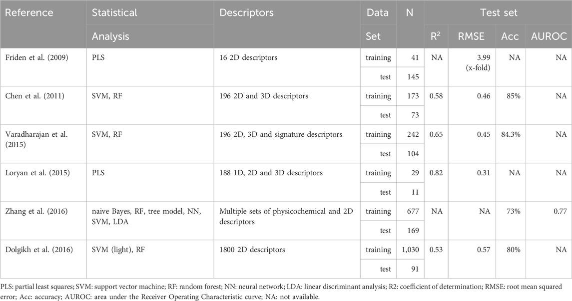
Table 1. Summary of QSAR models developed to predict Kp_uu,brain,ss. When more than one model was obtained in the same study, the values of the best model are presented.

The first QSAR model to predict Kp_uu,brain,ss was reported in 2009 by Fridén et al. (Fridén et al., 2009), based on a regression approach on a training set of 41 marketed drugs, with Kp_uu,brain,ss values derived from either the homogenate, brain slice or microdialysis techniques. As stated earlier, Kp_uu,brain,ss values can be estimated by combining an in vivo estimate of Kp_,brain in rat, and the in vitro estimation of binding parameters in both brain (f_u,brain) and plasma (f_u,plasma) (Eq. (2)).

${Kp}_{uu,brain}={Kp}_{brain}\frac{f_{u,brain}}{f_{u,plasma}}(2)$

In terms of predictive power, the model had a modest performance (Q² = 0.452 and RMSE = 3.49 in the test set), maybe due to the fact that only 16 descriptors were considered in the pool of possible predictors. Since this work initiated the in silico prediction of CNS unbound drug bioavailability, the publicly available dataset used in the study was later used for benchmarking purposes (Loryan et al., 2015; Dolgikh et al., 2016).

As shown in Table 1, an improvement in the Kp_uu,brain,ss predictive power was achieved by some of the QSAR models developed later, although reproducibility was somehow compromised by the fact that the corresponding datasets were totally or partially undisclosed (Chen et al., 2011; Loryan et al., 2015; Varadharajan et al., 2015; Dolgikh et al., 2016; Zhang et al., 2016). Furthermore, in order to expand the size of the dataset and thus achieve a wider applicability domain of the models, experimental Kp_uu,brain values were obtained by any of the three described methods, as well as in different conditions (steady-state/non-steady-state) and species (rat/mice). It should be noted that Table 1 is not exhaustive, as other models were developed until today. Nonetheless, they all have similar performance measures, and most of them still rely on totally or partially undisclosed (not publicly available) datasets (see, for example, Ma 2024 and citations therein).

The present study aimed to develop new in silico classification models to predict unbound drug brain bioavailability, following good practices of QSAR model development (Tropsha, 2010). The models reported here are based on a publicly available dataset, with a balanced training set and an explicit curation procedure. Our best models showed good performance on the hold-out dataset, and their predictive ability was externally validated in a prospective manner.

2 Materials and methods

2.1 Dataset compilation and characterization

After a careful bibliographic search, 711 Kp_uu,brain values corresponding to mice, rats, cynomolgus monkeys and humans were obtained from literature. Data sources are listed in the Supplementary Material. This dataset was then curated using different inclusion/exclusion criteria. As the first inclusion criterion, only the data values obtained under steady state conditions were considered. Secondly, only data obtained by homogenate, microdialysis, or brain slice techniques were considered for modeling purposes, while experimental data obtained by other techniques were disregarded. When the Kp_uu,brain,ss value of a compound was reported by more than one of the mentioned techniques, the data were prioritized according to the following hierarchy: 1) microdialysis; 2) brain slice and; 3) homogenate. After these selection criteria, the dataset was reduced to 157 compounds. The dataset compounds were then standardized using Standardizer 16.7.4.0 (ChemAxon) by following these actions: 1) Strip salts; 2) Remove Solvents; 3) Clear Stereo; 4) Remove Absolute Stereo; 5) Aromatize; 6) Neutralize; 7) Add Explicit Hydrogens; and 8) Clean 2D. Duplicated structures were removed.

Classification models were then trained and validated. A binary classification scheme (high/low CNS unbound BA) was defined using a cut-off value of Kp_uu,brain,ss of 0.4, which is a more conservative value than previously used ones (Zhang et al., 2016). Classification models were chosen over regression models to mitigate the noise linked to data obtained from different laboratories and different experimental settings (Talevi et al., 2012). Based on the previously defined cutoff criteria, 74 compounds were labeled as high CNS unbound BA compounds (Kp_uu,brain,ss ≥ 0.4) and 83 compounds were labeled as low CNS unbound BA compounds (Kp_uu,brain,ss < 0.4).

Except otherwise indicated, the R environment (R Core Team, 2021) was used for data analysis. Heatmaps illustrating the molecular dissimilarity between the compounds were built using ECFP_6 as a fingerprinting system, and Tanimoto distance as a dissimilarity metric. Principal Component Analysis (PCA) and frequency distribution were used to characterize the chemical diversity and chemical space covered by the dataset. For this, eight physicochemical descriptors (widely recognized as key parameters in drug discovery (Lipinski et al., 2001; Veber et al., 2002; Ritchie and Macdonald, 2009; Ward and Beswick, 2014) were used: molecular weight [MW], topological polar surface area [TPSA(Tot)], Moriguchi octanol-water partition coefficient [MLOGP], number of donor atoms for H-bonds [nHDon], number of acceptor atoms for H-bonds [nHAcc], number of rotatable bonds [RBN], number of rings (cyclomatic number) [nCIC] and sum of atomic van der Waals volumes [Sv].

2.2 Splitting the dataset into training and test sets

The compound dataset was divided as follows: a) a training set used to build the models, and b) an independent test set, to assess the predictive ability of the resulting models. To split the database into representative sets, we combined two clustering methodologies: first, a hierarchical clustering method using LibraryMCS software, (Chen and Guestrin, 2016) which relies on the Maximum Common Substructure to cluster a set of chemical structures without exhaustive pairwise comparison (Böcker, 2008). Subsequently, the resulting clustering was optimized using the k-means algorithm, randomly choosing k seeds from the clusters defined via LibraryMCS (R Core Team, 2021). This 2-step clustering was performed independently for the high and low CNS unbound BA categories.

Ideally, the training set should present a balanced class composition to prevent bias towards the prevalent category. Therefore, a balanced training set containing 110 compounds (55 from each category) was obtained by randomly taking 74% of each cluster from the high CNS unbound BA category and 66% of each cluster from the low CNS unbound BA category.

The previous dataset, which from now on will be called “complete dataset”, was further refined to examine the influence of substrates for ABC transporters on the modeling results, particularly over the descriptor selection step. For this purpose, we excluded compounds whose Kp_uu,brain,ss values had been obtained using the homogenate technique (which is subject to greater experimental variability and does not preserve tissue viability) and those compounds that according to the DrugBank database (Wishart et al., 2018) are substrates for P-glycoprotein (P-gp) and/or Breast Cancer Resistance Protein (BCRP), the two efflux transporters with the highest expression levels in the BBB (Liu et al., 2018). The previously described clustering procedure was applied to this “refined dataset” (67 compounds), resulting in a 38-compound training set (including 19 compounds with high and 19 with low CNS free drug BA) and a 29-compound test set (10 drugs with high and 19 with low CNS free drug BA), that is less likely to be influenced by active efflux mechanisms. The compositions of the completed and refined training and test sets are summarized in Table 2. Both datasets are included as Supplementary Material.

Table 2

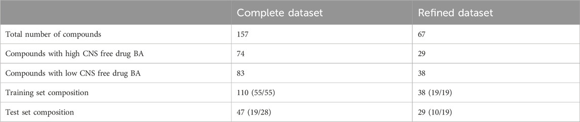
Table 2. Composition of the two datasets employed for modeling. Refined dataset excludes compounds whose Kp_uu,brain,ss value was obtained by the homogenate technique, as well as those labeled as P-gp or BCRP substrates in DrugBank.

2.3 Descriptor calculation

After curating the chemical structures, the molecular descriptors were computed. For this purpose, we used Dragon software (version 6.0; Milano Chemometrics, 2011) to calculate 3,668 conformation-independent descriptors. We removed molecular descriptors with missing values for any training set compound as well as descriptors with very low variance. These criteria yielded a pool of 1848 molecular descriptors that were used for modeling purposes.

2.4 Modeling methods

Models were built through a series of supervised machine learning algorithms: Support Vector Machine (SVM), Gradient Boosting Modeling (GBM), k-nearest neighbors (kNN), classificatory Partial Least Squares (cPLS), Random Forest (RF) and Extreme Gradient Boosting (XGBOOST), provided by the kernlab (Karatzoglou et al., 2004), gbm (Greenwell et al., 2020), caret (Kuhn et al., 2018), pls (Mevik and Wehrens, 2007), randomForest (Liaw and Wiener, 2002) and xgboost (Chen and Guestrin, 2016) R packages. A grid search with 5-times 10-fold cross-validation experiments was used in all cases to optimize the hyperparameters of the models. See Supplementary Material for a brief description of machine learning methods and hyperparameter grid search.

Deep Learning (DL) algorithm was additionally implemented using Keras (Chollet, 2015), a Python deep learning library, and Theano (The Theano Development Team, 2016) as a backend. The recommendations made by Ma et al (Ma et al., 2015) to develop the DL model were followed. The Scikit-learn library (Pedregosa et al., 2011) was used to implement 3-times 10-fold cross validation as a way to optimize the number of epochs during model training and avoid overfitting.

Additionally, an in-house random subspace-based modeling method (Alberca et al., 2018) was applied to obtain 1,000 random subsets of 200 potential independent variables (descriptors). This strategy reduces the probability of finding correlations by chance and allows stochastic exploration of the feature space. The Linear Discriminant Analysis (LDA) approach was then applied on each random subspace. A class label of 1 was used for compounds with Kp_uu,brain,ss ≥ 0.4, and a class label of 0 was used for compounds with Kp_uu,brain,ss < 0.4. A maximum variance inflation factor (VIF) value of 2 was set to exclude highly correlated descriptor pairs. A minimal 10:1 ratio between the number of training instances and the number of independent variables allowed in the model was used to prevent overfitting. The best models (up to five), based on the area under the ROC curve (AUROC) in the training set, were combined by the minimum and average operators (ensemble learning) to further improve their performance (Polikar, 2012). A description of this machine learning method is also provided in the Supplementary Material.

2.5 Applicability domain estimation

To avoid excessive extrapolation, similarity measurements were used to define the applicability domain of the model on the basis of the mean Euclidean distance between the training set compounds and each test compound. The distance of a test compound to its nearest neighbor in the training set is compared to a predefined applicability domain threshold (APD). If the distance exceeds this threshold, the prediction is considered unreliable. APD is calculated according to the following expression:

$APD=〈d〉+\mathrm{Z}\bullet {\mathrm{\sigma }}_{〈d〉}(3)$

The calculation of $〈d〉$ and σ is performed as follows. First, the mean Euclidean distance between all points of the training set is obtained. Then, using those distances lower than the mean, a second mean distance $〈d〉$ is computed, as well as its corresponding standard deviation ${\mathrm{\sigma }}_{〈d〉}$. Z is an empirical cutoff value, which was fixed at 0.5 (Zhang et al., 2006).

2.6 Evaluation of model performance

Accuracy (Acc), sensitivity (Se), specificity (Sp) and Matthews correlation coefficient (MCC) were computed to assess the performance of the obtained models. These parameters are defined by Eq. 4–7, where TP, FP, TN, and FN are the true positive rate, false positive rate, true negative rate, and false negative rate, respectively. Note that in this context, a compound with high CNS unbound BA will be considered a “positive” case.

$Se=\frac{TP}{TP+FN}(4)$

$Sp=\frac{TN}{FP+TN}(5)$

$Acc=\frac{TP+TN}{TP+FP+TN+FN}(6)$

$MCC=\frac{TP\cdot TN-FN\cdot FP}{\sqrt{\left(TP+FN\right)\cdot \left(TP+FP\right)\cdot \left(TN+FN\right)\cdot \left(TP+FP\right)}}(7)$

MCC is a measure of the quality of binary classifications, and it ranges between −1 and +1, with higher values indicating agreement between observed and predicted classes (Matthews, 1975). Receiving Operating Characteristic (ROC) curve analysis was also performed.

Once the best models were selected, the variable importance (VI) was established using different approaches depending on the modeling method (see Supplementary Material for further details).

2.7 Validation of the models

Each generated model was validated by:

› Leave-group-out cross-validation (CV). The training set was split randomly into 10 subsets of equal size; in each round of validation, one of these subsets was reserved and the remaining nine sets were used to retrain the model. It was ensured that each training example was removed at least once. The previous scheme was repeated 500 times to assess the model predictivity and robustness. In the case of DL, it was repeated only three times because of the computational cost.

› Hold-out validation. An independent test set (sampled from the complete and refined datasets, as mentioned in a previous section) was used to assess the predictive ability of the generated models. Visual inspection and two in-house small molecules clustering approximations, SOMoC and IRaPCA (Prada Gori et al., 2022) were used to detect possible chemical similarities across the misclassified compounds of the test set. SOMoC and IRaPCA default parameters were used.

2.8 Experimental validation

The predictive ability of the best classifier model derived from the complete dataset was validated prospectively by experimentally estimating the Kp_uu,brain,ss value of five compounds and comparing the predicted and the observed CNS unbound BA categories.

For this purpose, we experimentally determined the free fractions in plasma and brain of compounds whose Kp value was already reported (in steady-state and using rats as an animal model), but whose Kp_uu,brain,ss value had not been determined yet. As additional criteria, the compounds also had to be representative of both groups (high and low Kp_uu,brain, according to our predictions), and be commercially available in our country. To select such compounds, we performed a bibliographic search, and five drugs were selected: chlorpheniramine (Doan et al., 2004), lidocaine, 4-aminobenzoic acid (PABA) (Nakazono et al., 1991), ranitidine (Young et al., 1988) and theophylline (Yasuhara and Levy, 1988). Drugs were provided by Saporiti (Argentina).

The determination of the free drug fractions was performed by equilibrium dialysis at 37°C, with six independent replicas for each compound. The dialysis experiments were carried out in 6-well Costar Snapwell plates (Corning INC., Corning, NY, United States), by replacing the polycarbonate membrane of the inserts by dialysis membranes of 12 kDA molecular weight cut-off (Merck KGaA, Darmstadt, Germany).

In the plasma experiments, 700 μL of fresh rat plasma spiked with the compound under test (10 μM) were placed in the lower chamber (bottom of the well), and 300 μL of isotonic phosphate buffer solution pH 7.4 were placed in the upper chamber (insert). The system was allowed to equilibrate for at least 6 h on an orbital shaker at 37°C (Chen et al., 2019).

The f_u,plasma calculation was carried out following the method proposed by Banker et al. (Banker and Clark, 2008), which requires simultaneously carrying out an equilibrium control (replacing plasma with buffer), and the quantification of the analyte concentration in the acceptor compartments. Therefore, after 6 h, samples were taken from these compartments (sample and control) and analyzed using high performance liquid chromatography (HPLC). The free (unbound) drug fraction in plasma was then calculated as:

$f_u=\frac{R}{\left\{\frac{\left[\left(V_1+V_2\right)B-V_{2}R\right]}{V_1}\right\}}(8)$

Where R is the drug concentration in the samples dialysate, V₁ and V₂ are the volumes of the donor and acceptor chambers, respectively, and B represents the concentration of the analyte in the control dialysate.

A similar protocol was followed to estimate the free fraction in the brain, except that rat brain homogenate was used instead of plasma. For the preparation of the homogenate, rat brains were harvested and immediately diluted in twice their weight of 100 mM sodium phosphate buffer solution pH 7.4. Homogenization was carried out with a Pro Scientific Bio-Gen Pro200 high shear homogenizer (PRO Scientific Inc., Oxford, CT, United States), for at least 1 min. Subsequently, the dialysis was performed as in the case of plasma, but placing 700 μL of brain homogenate in the donor compartment, spiked with the analyte to reach a 1 μM concentration. The f_u,brain values obtained according to Equation 8 were corrected for the dilution of the tissue (Kalvass et al., 2002). For a dilution factor D (in our experiments, 3), the correction proposed by Kalvass et al. is:

$f_{u,undiluted}=\frac{\raisebox{1ex}{$1$}\!\left/ \!\raisebox{-1ex}{$D$}\right.}{\left(\left(\raisebox{1ex}{$1$}\!\left/ \!\raisebox{-1ex}{$f_{u,diluted}$}\right.\right)-1\right)+\raisebox{1ex}{$1$}\!\left/ \!\raisebox{-1ex}{$D$}\right.}(9)$

Finally, the Kp_uu,brain,ss value of each compound was obtained by means of Equation 2, using the f_u values experimentally determined and the bibliographic values of Kp.

2.8.1 Chromatographic methods

After the dialysis experiments, analytical determinations were carried out in a Dionex Ultimate 3000 UHPLC apparatus (Thermo Scientific, Sunnyvale, CA, United States), equipped with a dual gradient ternary pump (DGP-3000) and a diode array detector (DAD-3000). A Hibar C18 RP column (125 mm × 4 mm, 5 μm, Merck KGaA, Darmstadt, Germany) was used as stationary phase. The mobile phase and the wavelength of detection for each compound were: a mixture of methanol and 50 mM KH₂PO₄ buffer pH 2.5 (40:60) for chlorpheniramine, with detection at 261 nm; a mixture of methanol and 50 mM KH₂PO₄ pH 2.5 buffer solution (25:75) for lidocaine, with detection at 220 nm; a mixture of methanol and 50 mM KH₂PO₄ pH 2.5 buffer solution (5:95) for PABA, with detection at 281 nm; a mixture of methanol and 20 mM Na₂HPO₄ pH 7.4 buffer solution (40:60) for ranitidine, with detection at 316 nm, and; a mixture of methanol and 20 mM KH₂PO₄ pH 2.5 buffer solution (20:80) for theophylline, with UV detection at 271 nm. In all cases, the equipment was operated isocratically at room temperature, with a mobile phase flow of 1 mL/min. HPLC grade Methanol and MiliQ water were used for the preparation of mobile phase. Other reagents were of analytical grade.

Prior to the injections (in duplicate), the samples were centrifuged at 10,000 rpm for 5 min and injected directly or diluted with premixed mobile phase, in order to reach concentrations within the linear range of the methods. A manual injector (Rheodyne, CA, United States) with a 20 μL fixed loop was used for injection.

3 Results

711 data of compounds with their corresponding Kp_uu,brain values were retrieved from literature. Of these, 276 data were disregarded because they have been obtained under non-steady state conditions. 11 data were excluded since they corresponded to determinations in cerebrospinal fluid (not brain) or because they did not correspond to the microdialysis, slice or homogenate techniques. Finally, 267 repeated values were discarded, retaining data for 157 compounds. The heatmap shown in Figure 1 provides graphical evidence of the molecular diversity of the compounds that compose the complete dataset. The predominant color indicates a wide chemical diversity, which is a desirable feature that contributes to ensure a wide applicability domain of the models derived from this dataset.

Figure 1

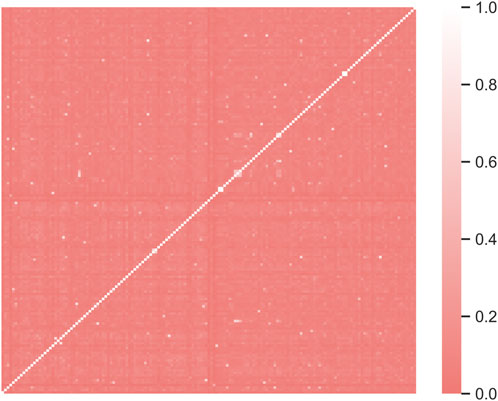
Figure 1. The heatmap illustrates the molecular diversity of the compounds in the complete dataset (157 compounds). Dark coral regions indicate dissimilarity. Morgan fingerprints (radius 3) were used as molecular fingerprinting system and Tanimoto distance was used for dissimilarity calculations. RDKIT and Seborn Python packages were used to compute similarity and build the heatmap, respectively.

The data distribution among the physicochemical space of the complete dataset can be visualized in the PCA and histograms plots (Figures 2, 3).

Figure 2

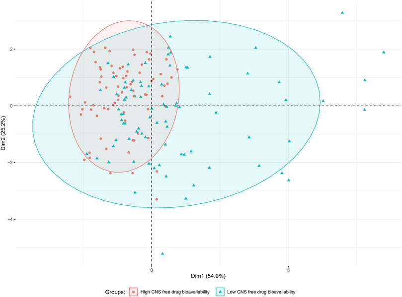
Figure 2. PCA plot of the complete dataset (157 compounds) based on eight physicochemical descriptors (MW; TPSA(Tot); MLogP; nHDon; nHAcc; RBN; nCIC and Sv). Data points are colored according to their category (green triangles and red circles for low and high CNS free BA, respectively). The drawn ellipses assume a multivariate normal distribution of the data by group with a confidence level of 0.9; they are drawn to facilitate the observation of the degree of overlapping between both groups.

Figure 3

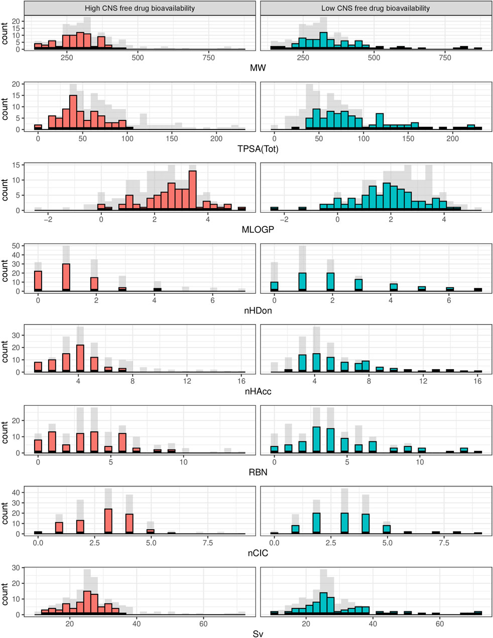
Figure 3. Histograms showing the frequency distribution of the selected physicochemical descriptors across the complete dataset. Gray bars represent the complete dataset, while red and green bars correspond to high and low CNS unbound BA categories, in that order.

From the PCA displayed in Figure 2, constructed using the eight physicochemical descriptors listed in the methodological section, it is clear that the distribution of those properties is wider among the low CNS free drug bioavailability group of compounds (low CNS BA, green triangles in the figure) than for the high CNS free drug bioavailability group (high CNS BA, red circles in the figure). For the latter, which represent our “active” or pursued group, it can be seen that the physicochemical region covered is narrower, and fully embedded within the region covered by the low CNS BA group. The histograms in Figure 3 represent the distribution frequency of the eight selected physicochemical descriptors across the complete dataset. Green and red bars represent low and high CNS BA groups, respectively, whereas gray bars represent the sum of both categories. As expected, the frequency distributions of Figure 3 agree with the previously discussed PCA analysis, with the low CNS BA compounds displaying wider diversity, and a significant overlap between both groups.

Whereas the distribution of the compounds in the chemical space is very informative (for instance, it tells us that some regions of the chemical space are very unlikely to be occupied by compounds with high free CNS BA), the overlapping regions between both groups pose a major challenge for the development of models to predict Kp_uu,brain,ss. It was thus decided to explore a large feature pool as well as several machine learning algorithms to overcome this obstacle.

Table 3 summarizes the performance of the models developed using the complete dataset. The table displays the AUROC and Acc values for both the training and the test sets, as well as the MCC, Se and Sp for the test set. These parameters serve to evaluate the classificatory ability of the models, and to select the best-performing algorithm. The results of the 10-fold CV, in terms of mean accuracy on the hold out examples of each leave-group-out round, are also shown. The value of the metrics shown in the table correspond to the score cutoff value that maximizes MCC.

Table 3

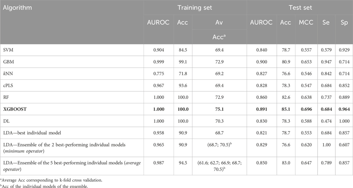
Table 3. Performance metrics of the models derived from the complete dataset. The selected algorithm has been highlighted in bold letters (best model, according to the values of MCC and AUROC in the test set).

In terms of explanatory power (i.e., the ability to accurately classify the training examples), the best-performing algorithms are either extremely flexible ones (DL) or those that resort to some sort of ensemble learning and produce a meta-classifier (RF, GBM, XGBOOST, and the 5-model ensemble of our in-house selective combination of linear classifiers). All of them produce perfect or almost perfect classification of the training set compounds. However, judging from the results of the internal and external cross-validations, it is evident that all the algorithms, with the sole exception of kNN (whose performance on the test set is above that on the training set), have resulted in overfitting. Remarkably, the algorithms with best explanatory power are the ones that seem to present a higher degree of overfitting (as reflected by the difference between Acc in the training set minus Acc in the test set, always positive except for kNN, see Figure 4). This is in line with the well-known fact that using disproportionally flexible algorithms often results in memorization of features of the training set and poor predictive ability.

Figure 4

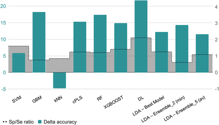
Figure 4. The green bars represent the value of the difference between the accuracy in the training set minus the accuracy in the test set, for each algorithm or meta-algorithm (scale in the left vertical axis). The gray bars represent the Sp/Se ratio (scale in the right vertical axis).

On the other hand, the algorithms with modest performance are the ones with less overfitting (LDA) or no overfitting at all (kNN). This may reflect, in part, that the sampling approach that we used to split the dataset has not provided good results (training and test sets that present a similar coverage in the chemical space). However, it is more likely that the best-performing algorithms are excessively flexible to deal with our small dataset without some degree of overfitting, as exemplified by the DL model, which provides the best performance in the training set but one of the worst in the test set. Importantly, XGBOOST (in bold in Table 3) matches the explanatory power of DL but also shows the best performance in the external validation, for which an accuracy above 85% was observed, similar to the one of the best classification model shown in Table 1. Based on this analysis, the XGBOOST model was chosen as the best-performing one and it was used to predict the categories of those compounds submitted to experimental confirmation of their unbound brain BA.

Regarding the Sp and Se ratio, kNN, LDA (5-model ensemble) and RF are the methods that provide the most balanced relationship between Sp and Se (i.e., Sp/Se ratio closest to one, see Figure 4) at the cutoff score value that maximizes MCC. It is worth highlighting that our 5-model ensemble of linear classifiers greatly improved the robustness of the predictions, judging from the poor behavior in the cross-validation of the individual models that compose the ensemble and the good accuracy (83%) of the combined models in the test set. On the other hand, in the context of CNS drugs R&D, the focus will be on compounds that present good unbound BA in the brain; therefore, due to its Sp/Se ratio >1, XGBOOST results in a conservative model (that is, associated with a low rate of false positives), and therefore useful for optimizing the use of resources.

According to the applicability domain assessment, 44 out of 47 compounds in the test set belong to the applicability domain and thus have been reliably predicted. It should be noted that none of the compounds incorrectly classified by the model were out of the applicability domain. Furthermore, the compounds used for the prospective experimental validation also fall within the application domain of the best model.

The seven compounds that were mispredicted by the XGBOOST model are shown in Figure 5. No clear chemical relationship can be observed across them, apart from the obvious structural relationship between trazodone and ziprasidone. To detect possible structural patterns between these compounds beyond the ones emerging from visual inspection, they were subjected to clustering exercises using two in-house clustering approximations, SOMoC and IRaPCA. SOMoC allocated the seven compounds to three different clusters (three compounds in one cluster, three compounds in another, and the remaining compound in a third cluster). Similarly, IRaPCA allocated the seven compounds to different clusters or subclusters, except for trazodone and ziprasidone, which were assigned to the same subclusters, consistently with visual inspection. Regarding the incorrect predictions by the cPLS and RF models derived from the refined dataset, each of these models misclassified four compounds from the test set, with three common misclassifications (probenecid, gabapentin, and trifluoperazine). According to DrugBank, several of the misclassified molecules (e.g., trifluoperazine, probenecid, ondasetron) have reported interactions with different transporters that are expressed at the BBB, including ABC efflux transporters, which may have contributed to their misclassification by the models emerging from the refined dataset.

Figure 5

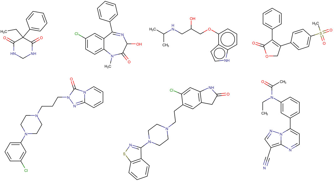
Figure 5. Structures of the seven incorrectly classified test set compounds by the best model derived from the complete dataset.

Table 4 details the results from the experimental validation. Our external validation set was based on five compounds, three of low and two of high Kp_uu,brain,ss. Four of these compounds were correctly predicted, confirming the predictive power of the models. Of note, the accuracy on this small set of compounds (80%) is right between the mean Acc in the cross-validation rounds (75%) and the Acc in the test set (85%). Although the size of this set of compounds is clearly small, the results of the internal, external and experimental validation seem fairly comparable.

Table 4

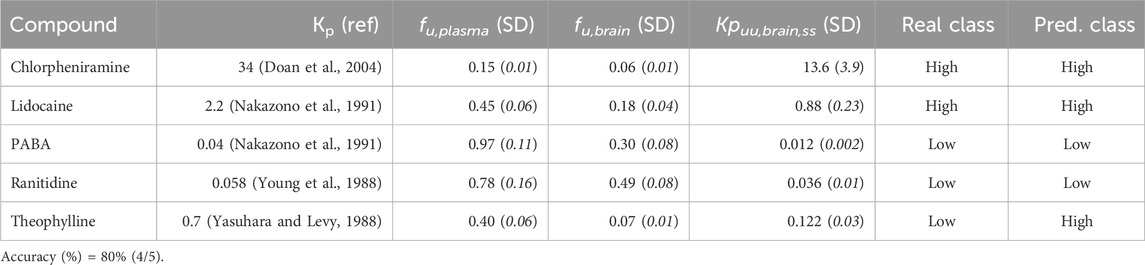
Table 4. Performance of the best model (XGBOOST) in the external validation set.

Finally, when working with the refined dataset (i.e., after removing the compounds which are known substrates of the ABC polyspecific transporters with the highest expression levels at the BBB, P-gp and BCRP), the best-performing algorithms differ from those that performed best on the complete dataset (Table 5), as expected due to the fact that removing the transporter substrates greatly modifies the characteristics of the dataset (notably, its size). According to their performance on the test set, the best algorithms were cPLS and RF, which yielded identical results in terms of Acc (86.2), MCC (0.716), Se (0.9) and Sp (0.842). More interesting, however, is the change in the pattern of relevant descriptors selected by the models trained with the complete or the refined dataset. Figure 6 shows the comparative distribution of the most relevant descriptors and descriptor classes selected by the models in both datasets. To establish the “relevance”, descriptors were listed in descending order according to the number of times that they were selected as one of the 20-most relevant variables by the different algorithms, and the first 20 were included in the figure. The cPLS and RF models derived from the refined dataset have been applied in the prediction of the five compounds subjected to experimental confirmation. Surprisingly, and despite ranitidine is a known P-gp substrate, the five compounds were correctly predicted by the “refined” models.

Table 5

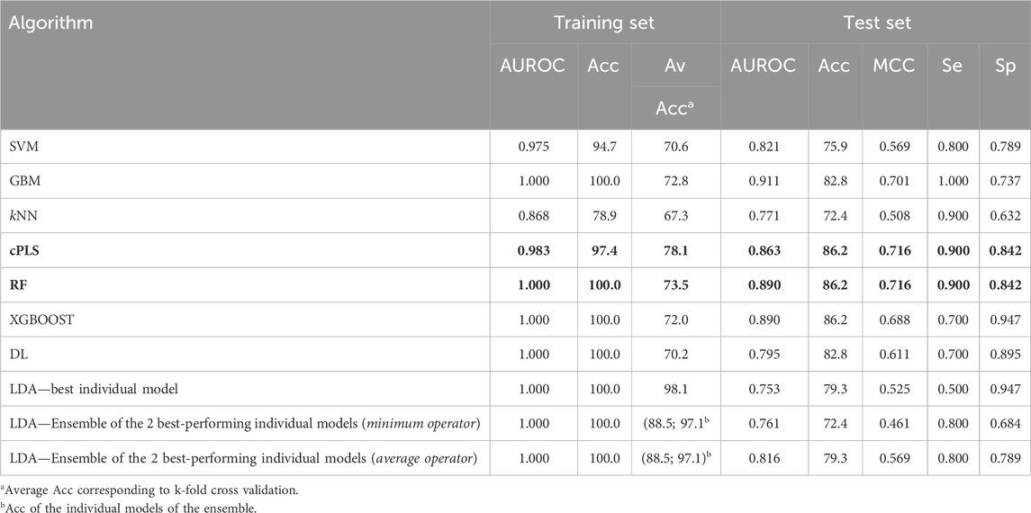
Table 5. Performance metrics of the models derived from the refined dataset. The best performing algorithms (according to the values of MCC and AUROC in the test set) are highlighted in bold letters.

Figure 6

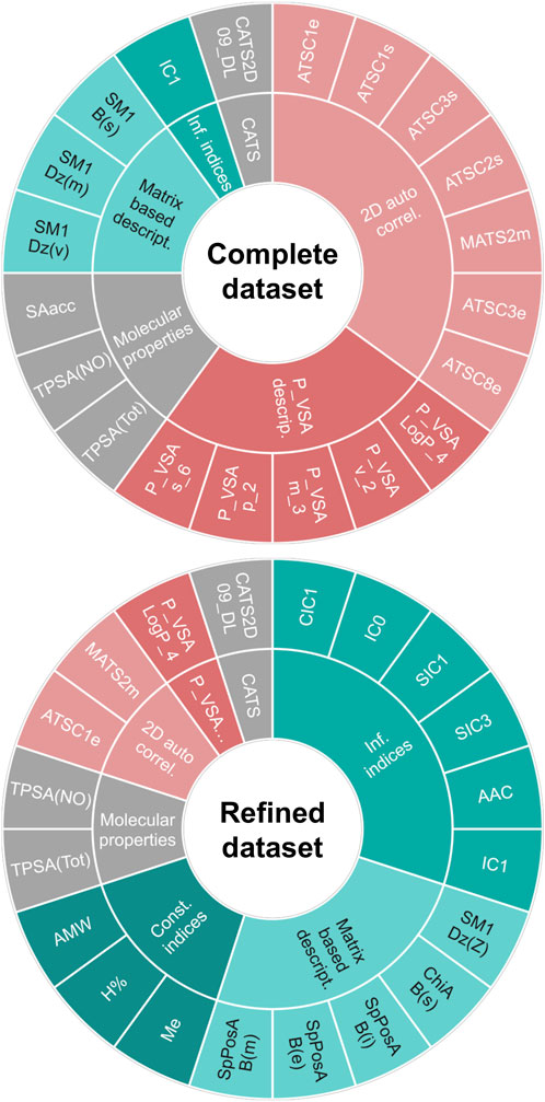
Figure 6. Main descriptors (first 20) selected by the models trained in the complete dataset (up) and in the refined dataset (down). A table indicating the meaning of each descriptor is provided as Supplementary Material.

4 Discussion

It is probable that several factors may have contributed to the good performance of the classification models developed in the present work. Among them, we can cite the different machine learning algorithms used to find the correlation patterns between the data, as well as the large number of molecular descriptors used to characterize the dataset. The careful curation of the complete dataset was possibly a key factor to obtain accurate machine learning models. We have implemented a “less is more” approximation, choosing the use of a small-size but high-quality dataset to derive and validate our models, instead of a large dataset with data of highly variable quality. It is worth noting that the dataset comprised data on unbound partition coefficients obtained from different species, including rodents and primates, which may constitute a source of uncertainty because of inter-species variability. However, we expect that the use of classification models mitigates, at least partially, the noise associated with this issue, especially if inter-species variability does not result in mislabeling of the compound class.

In relation to the refined dataset, it should be emphasized that absence of information in Drugbank regarding whether a specific compound is a substrate of an ABC transporter, does not strictly mean that this compound is not substrate for such transporters, but rather that no evidence exists so far on it being a substrate. The compounds that comprise the refined dataset, on the other hand, may be substrates of other (efflux or influx) transporters not considered in the analysis. In any case, the 42 compounds removed from the complete dataset were predominantly from the low CNS BA group (27 compounds), as expected for a substrate of BCRP or P-gp.

As mentioned in the precedent section, there was, for almost all the machine learning algorithms used and for both the complete and refined datasets, a general trend to observe higher explanatory than predictive power (i.e., higher performance on internal than external data). This may have arisen from some degree of overfitting, as reflected by the fact that the differences in internal and external accuracies were accentuated for very flexible approximations such as gradient boosting or DL algorithms. Another possible explanation to this phenomenon may be related to the fact that we have preferred to use balanced training sets to avoid biased models favoring the majority class. This has resulted, however, in the enrichment of the dataset’s majority class in the test set, i.e., relatively highly imbalanced test sets. It is possible that imbalanced training sets may provide models with better predictivity on imbalanced external datasets, especially if the predictivity is not even across classes. However, as our main focus is the prediction of bioavailability of active scaffolds for the potential treatment of CNS conditions, we preferred to train our models from balanced training sets so that they are not biased towards the majority class (here, the compounds with low CNS unbound BA) so that valuable scaffolds with high CNS unbound BA are not disregarded due to a misprediction related to biased models.

When analyzing the patterns of descriptors included in the models derived from the complete and refined dataset (Figure 5), they included several descriptors linked to molecular properties that are relevant for the passive movement of a compound across the BBB, such as surface area (e.g., TPSA(Tot), TPSA(NO)), molecular weight or size (e.g., AMW, P_VSA_m_3) and lipophilicity (e.g., P_VSA_LogP_4), among others (Fridén et al., 2009). However, there are remarkable differences across both datasets in the descriptors incorporated to the models: in the complete dataset the most frequent descriptors correspond to 2D autocorrelations, whereas in the refined dataset information indices predominate. Autocorrelation descriptors encode the relative distribution of atomic properties (e.g., electronegativity, polarizability or atomic mass) in a given molecule, and might be conceptually related with pharmacophoric patterns, although in 2D autocorrelations topological distances are considered instead of geometrical distances (Sliwoski et al., 2016). Thus, it is reasonable that this type of descriptors appears more frequently in models derived from a dataset that includes substrates of drug transporters, as they may reflect molecular features that facilitate recognition by such transporters. Contrariwise, the refined dataset, which excludes substrates for two polyspecific efflux transporters (P-gp and BCRP) with high expression levels at the BBB, is more likely to produce models with higher incidence of descriptors related to passive diffusion across the BBB, with less incidence of pharmacophore-like descriptors. In particular, information indices reflect information content associated to the subgraphs that may be derived from a molecule. Their values reflect the complexity of the molecules (in terms of bond types and atomic composition) and their symmetry/asymmetry. Because of the rather limited number of atoms that compose organic compounds, it can be expected that compounds with high information content will possess several heteroatoms and will thus be less likely to permeate the BBB passively. Consistently, these indices appear in the models associated with negative loads or coefficients, and thus their increment (i.e., greater molecular complexity) is associated with the low CNS unbound BA class. Furthermore, the second more abundant group of relevant descriptors in the refined dataset are matrix-based descriptors, which reflect complex structural patterns, such as molecular shape, size, cyclicity and branching (Grisoni et al., 2017). In other words, by removing the P-gp/BCRP substrates, the group of main descriptors is enriched in chemical features that may be linked to passive diffusion, showing that the modeling approaches are somehow sensitive to the mechanism of passage through the BBB.

Interestingly, the best model obtained from the complete dataset (XGBOOST model) provided accurate classifications for four of the five compounds used for prospective validation through the homogenate approach, while the best models obtained from the refined dataset (cPLS and RF models) accurately predicted the five compounds. Although the number of compounds used for the prospective validation is small and does not allow any generalization, the models obtained from the refined dataset outperformed the ones obtained from the complete dataset for this limited set of compounds, even when one of them (ranitidine) is a known P-gp substrate and despite the refined dataset does not include homogenate data. This may possibly indicate that the passage of these five compounds through the BBB is majorly governed by a simple diffusion phenomenon that, as previously mentioned, is better captured by the molecular descriptors incorporated to the refined models.

5 Conclusion

We report a diversity of classifiers to predict unbound drug bioavailability in the brain, which in general displayed good performance. We have chosen to use a dataset of relatively limited size which was however subjected to careful curation, including compounds with Kp_uu,brain,ss values determined either by microdialysis, the brain slice and the homogenate techniques, and excluding data points non representative of the steady state conditions. Such data curation could have served to reduce noise in our final dataset (“complete dataset”). Based on the high variability reported for homogenate data, we conceived a second dataset (“refined dataset”) from which homogenate data was omitted. This dataset also excludes reported substrates for ABC efflux transporters P-gp and BCRP; therefore, it was expected that the models obtained from the refined would be much more influenced by molecular descriptors associated with simple diffusion through the BBB. These decisions may, in turn, limit the applicability domain of our models, which is expected to be narrower when using training data of limited size. The best models derived from the complete and the refined datasets have obtained good predictivity using a small prospective validation set. The models inferred from the refined dataset achieved better performance in the prospective validation.

It is convenient to underline that Kp_uu,brain,ss experimental data for all the compounds used for modeling and validation purposes are publicly available since they have been published in scientific literature (and are also provided as supplementary online resources). We have also provided our datasets, code, and search range for hyperparameters; accordingly, it is possible to reproduce and even refine or expand our modeling approaches.

While our models could prove useful to assist the drug discovery stage when seeking for CNS therapeutics, it should be remembered that, while the free drug BA influences the chances for a drug candidate to become a CNS approved drug, the interplay between BA and intrinsic potency of the drug should always be taken into consideration. Low permeation of a drug could occasionally be compensated by high potency: if very low therapeutic concentrations are required, they may be achieved despite poor CNS bioavailability.

Data availability statement

The original contributions presented in the study are included in the article/Supplementary Material, further inquiries can be directed to the corresponding author.

Ethics statement

The animal study was approved by CICUAL, Facultad de Ciencias Exactas, UNLP. The study was conducted in accordance with the local legislation and institutional requirements.

Author contributions

JM: Data curation, Formal Analysis, Investigation, Methodology, Software, Validation, Visualization, Writing–original draft. MR: Conceptualization, Formal Analysis, Methodology, Resources, Supervision, Validation, Writing–original draft, Writing–review and editing. RS: Resources, Supervision, Validation, Writing–review and editing. AT: Conceptualization, Data curation, Formal Analysis, Funding acquisition, Project administration, Resources, Supervision, Visualization, Writing–original draft, Writing–review and editing.

Funding

The author(s) declare financial support was received for the research, authorship, and/or publication of this article. The present work was supported by Argentine grants from CONICET (National Council for Science and Technology, PIP 0498), The National Agency of Scientific and Technological Promotion (ANPCyT, PICT 2011-2116, PICT 2013-3175, PICT 2019-1075), UNLP (National University of La Plata, 11/X729 and PRH 5.2).

Acknowledgments

The authors thank the National University of La Plata (UNLP) and CONICET. They also thank the reviewers, whose comments have served to improve the original manuscript.

Conflict of interest

The authors declare that the research was conducted in the absence of any commercial or financial relationships that could be construed as a potential conflict of interest.

The author(s) declared that they were an editorial board member of Frontiers, at the time of submission. This had no impact on the peer review process and the final decision.

Publisher’s note

All claims expressed in this article are solely those of the authors and do not necessarily represent those of their affiliated organizations, or those of the publisher, the editors and the reviewers. Any product that may be evaluated in this article, or claim that may be made by its manufacturer, is not guaranteed or endorsed by the publisher.

Supplementary material

The Supplementary Material for this article can be found online at: https://www.frontiersin.org/articles/10.3389/fddsv.2024.1360732/full#supplementary-material

SUPPLEMENTARY DATA SHEET 1 | Brief description of machine learning methods and hyperparameter grid search.

SUPPLEMENTARY DATA SHEET 2 | Datasets and list of data sources.

SUPPLEMENTARY DATA SHEET 3 | Definition of molecular descriptors.

SUPPLEMENTARY DATA SHEET 4 | Code for in house method.

References

Alberca, L. N., Sbaraglini, M. L., Morales, J. F., Dietrich, R., Ruiz, M. D., Pino Martínez, A. M., et al. (2018). Cascade ligand- and structure-based virtual screening to identify new trypanocidal compounds inhibiting putrescine uptake. Front. Cell. Infect. Microbiol. 8, 173. doi:10.3389/fcimb.2018.00173

PubMed Abstract | CrossRef Full Text | Google Scholar

Banker, M., and Clark, T. (2008). Plasma/serum protein binding determinations. Curr. Drug Metab. 9 (9), 854–859. doi:10.2174/138920008786485065

PubMed Abstract | CrossRef Full Text | Google Scholar

Benjamin, B., Sahu, M., Bhatnagar, U., Abhyankar, D., and Srinivas, N. R. (2012). The observed correlation between in vivo clinical pharmacokinetic parameters and in vitro potency of VEGFR-2 inhibitors. Arzneimittelforschung 62 (4), 194–201. doi:10.1055/s-0031-1299772

PubMed Abstract | CrossRef Full Text | Google Scholar

Böcker, A. (2008). Toward an improved clustering of large data sets using maximum common substructures and topological fingerprints. J. Chem. Inf. Model. 48 (11), 2097–2107. doi:10.1021/ci8000887

PubMed Abstract | CrossRef Full Text | Google Scholar

Chen, H., Winiwarter, S., Fridén, M., Antonsson, M., and Engkvist, O. (2011). In silico prediction of unbound brain-to-plasma concentration ratio using machine learning algorithms. J. Mol. Graph. 29 (8), 985–995. doi:10.1016/j.jmgm.2011.04.004

PubMed Abstract | CrossRef Full Text | Google Scholar

Chen, T., and Guestrin, C. (2016). “XGBoost: a scalable tree boosting system,” in Proceedings of the 22nd ACM SIGKDD international conference on knowledge discovery and data mining (ACM), 785–794. doi:10.1145/2939672.2939785

CrossRef Full Text | Google Scholar

Chen, Y. C., Kenny, J. R., Wright, M., Hop, C. E. C. A., and Yan, Z. (2019). Improving confidence in the determination of free fraction for highly bound drugs using bidirectional equilibrium dialysis. J. Pharm. Sci. 108 (3), 1296–1302. doi:10.1016/j.xphs.2018.10.011

PubMed Abstract | CrossRef Full Text | Google Scholar

Chollet, F. (2015). Keras. Avaliable at: https://keras.io (Accessed November 17, 2023).

Google Scholar

Cook, D., Brown, D., Alexander, R., March, R., Morgan, P., Satterthwaite, G., et al. (2014). Lessons learned from the fate of AstraZeneca’s drug pipeline: a five-dimensional framework. Nat. Rev. Drug Discov. 13 (6), 419–431. doi:10.1038/nrd4309

PubMed Abstract | CrossRef Full Text | Google Scholar

Doan, K. M., Wring, S. A., Shampine, L. J., Jordan, K. H., Bishop, J. P., Kratz, J., et al. (2004). Steady-state brain concentrations of antihistamines in rats: interplay of membrane permeability, P-glycoprotein efflux and plasma protein binding. Pharmacology 72 (2), 92–98. doi:10.1159/000079137

PubMed Abstract | CrossRef Full Text | Google Scholar

Dolgikh, E., Watson, I. A., Desai, P. V., Sawada, G. A., Morton, S., Jones, T. M., et al. (2016). QSAR model of unbound brain-to-plasma partition coefficient, Kp,uu,brain: incorporating P-glycoprotein efflux as a variable. J. Chem. Inf. Model. 56 (11), 2225–2233. doi:10.1021/acs.jcim.6b00229

PubMed Abstract | CrossRef Full Text | Google Scholar

Fridén, M., Bergström, F., Wan, H., Rehngren, M., Ahlin, G., Hammarlund-Udenaes, M., et al. (2011). Measurement of unbound drug exposure in brain: modeling of pH partitioning explains diverging results between the brain slice and brain homogenate methods. Drug Metab. Dispos. 39 (3), 353–362. doi:10.1124/dmd.110.035998

PubMed Abstract | CrossRef Full Text | Google Scholar

Fridén, M., Winiwarter, S., Jerndal, G., Bengtsson, O., Wan, H., Bredberg, U., et al. (2009). Structure−Brain exposure relationships in rat and human using a novel data set of unbound drug concentrations in brain interstitial and cerebrospinal fluids. J. Med. Chem. 52 (20), 6233–6243. doi:10.1021/jm901036q

PubMed Abstract | CrossRef Full Text | Google Scholar

Greenwell, B., Boehmke, B., Cunningham, J., and Developers, G. B. M. (2020). Gbm: generalized boosted regression models. R pacakge version 2.1.8. Avaliable at: https://cran.r-project.org/web/packages/gbm/index.html (Accessed November 21, 2023).

Google Scholar

Grisoni, F., Reker, D., Schneider, P., Friedrich, L., Consonni, V., Todeschini, R., et al. (2017). Matrix-based molecular descriptors for prospective virtual compound screening. Mol. Inf. 36 (1-2), 1600091. doi:10.1002/minf.201600091

PubMed Abstract | CrossRef Full Text | Google Scholar

Kalvass, J. C., Maurer, T. S., Cory Kalvass, J., and Maurer, T. S. (2002). Influence of nonspecific brain and plasma binding on CNS exposure: implications for rational drug discovery. Biopharm. Drug Dispos. 23 (8), 327–338. doi:10.1002/bdd.325

PubMed Abstract | CrossRef Full Text | Google Scholar

Karatzoglou, A., Smola, A., Hornik, K., and Zeileis, A. (2004). Kernlab—an S4 package for kernel methods in R. J. Stat. Softw. 11 (9), 1–20. doi:10.18637/jss.v011.i09

CrossRef Full Text | Google Scholar

Keaney, J., and Campbell, M. (2015). The dynamic blood-brain barrier. FEBS J. 282 (21), 4067–4079. doi:10.1111/febs.13412

PubMed Abstract | CrossRef Full Text | Google Scholar

Kielbasa, W., and Stratford, R. E. (2015). “Microdialysis to assess free drug concentration in brain,” in Blood-brain barrier in drug discovery. Editors L. Di, and E. H. Kerns (Hoboken, NJ: John Wiley & Sons, Inc.), 351–364.

CrossRef Full Text | Google Scholar

Kuhn, M., Wing, J., Weston, S., Williams, A., Keefer, C., Engelhardt, A., et al. (2018). Caret: classification and Regression Training. R package version 6.0-84. R package version 6.0. Avaliable at: https://cran.r-project.org/web/packages/caret/index.html (Accessed November 20, 2023).

Google Scholar

Lanevskij, K., Japertas, P., and Didziapetris, R. (2013). Improving the prediction of drug disposition in the brain. Exp. Op. Drug Metab. Toxicol. 9 (4), 473–486. doi:10.1517/17425255.2013.754423

PubMed Abstract | CrossRef Full Text | Google Scholar

Liaw, A., and Wiener, M. (2002). Classification and regression by random forest. R. news 2 (3), 18–22. Avaliable at: https://CRAN.R-project.org/doc/Rnews/.

Google Scholar

Lipinski, C. A., Lombardo, F., Dominy, B. W., and Feeney, P. J. (2001). Experimental and computational approaches to estimate solubility and permeability in drug discovery and development settings. Adv. Drug Deliv. Rev. 46 (1-3), 3–26. doi:10.1016/s0169-409x(00)00129-0

PubMed Abstract | CrossRef Full Text | Google Scholar

Liu, H., Dong, K., Zhang, W., Summerfield, S. G., and Terstappen, G. C. (2018). Prediction of brain:blood unbound concentration ratios in CNS drug discovery employing in silico and in vitro model systems. Drug disc. Today 23 (7), 1357–1372. doi:10.1016/j.drudis.2018.03.002

PubMed Abstract | CrossRef Full Text | Google Scholar

Loryan, I., Fridén, M., and Hammarlund-Udenaes, M. (2013). The brain slice method for studying drug distribution in the CNS. Fluids Barriers CNS 10 (1), 6. doi:10.1186/2045-8118-10-6

PubMed Abstract | CrossRef Full Text | Google Scholar

Loryan, I., Sinha, V., Mackie, C., Van Peer, A., Drinkenburg, W. H., Vermeulen, A., et al. (2015). Molecular properties determining unbound intracellular and extracellular brain exposure of CNS drug candidates. Mol. Pharm. 12 (2), 520–532. doi:10.1021/mp5005965

PubMed Abstract | CrossRef Full Text | Google Scholar

Ma, J., Sheridan, R. P., Liaw, A., Dahl, G. E., and Svetnik, V. (2015). Deep neural nets as a method for quantitative structure–activity relationships. J. Chem. Inf. Model. 55 (2), 263–274. doi:10.1021/ci500747n

PubMed Abstract | CrossRef Full Text | Google Scholar

Ma, Y., Jiang, M., Javeria, H., Tian, D., and Du, Z. (2024). Accurate prediction of Kp,_uu,brain based on experimental measurement of Kp,^brain and computed physicochemical properties of candidate compounds in CNS drug discovery. Heliyon 10, e24304. doi:10.1016/j.heliyon.2024.e24304

PubMed Abstract | CrossRef Full Text | Google Scholar

Matthews, B. W. (1975). Comparison of the predicted and observed secondary structure of T4 phage lysozyme. Biochim. Biophys. Acta. 405 (2), 442–451. doi:10.1016/0005-2795(75)90109-9

PubMed Abstract | CrossRef Full Text | Google Scholar

Mevik, B. H., and Wehrens, R. (2007). The pls package: principal component and partial least squares regression in R. J. Stat. Stoftw. 18, 18. doi:10.18637/jss.v018.i02

CrossRef Full Text | Google Scholar

Morales, J. F., Scioli Montoto, S., Fagiolino, P., and Ruiz, M. E. (2017). Current state and future perspectives in QSAR models to predict blood- brain barrier penetration in central nervous system drug R&D. Mini-Rev. Med. Chem. 17 (3), 247–257. doi:10.2174/1389557516666161013110813

PubMed Abstract | CrossRef Full Text | Google Scholar

Nakazono, T., Murakami, T., Higashi, Y., and Yata, N. (1991). Study on brain uptake of local anesthetics in rats. J. Pharmacobiodyn. 14 (11), 605–613. doi:10.1248/bpb1978.14.605

PubMed Abstract | CrossRef Full Text | Google Scholar

Pedregosa, F., Varoquaux, G., Gramfort, A., Michel, V., Thirion, B., Grisel, O., et al. (2011). Scikit-learn: machine learning in Python. J. Mach. Learn. Res. 12, 2825–2830.

Google Scholar

Polikar, R. (2012). in Ensemble learning" in ensemble machine learning. Editors C. Zhang, and Y. Ma (New York, NY: Springer), 1–34. doi:10.1007/978-1-4419-9326-7_1

CrossRef Full Text | Google Scholar

Prada Gori, D. N., Llanos, M. A., Bellera, C. L., Talevi, A., and Alberca, L. N. (2022). iRaPCA and SOMoC: development and validation of web applications for new approaches for the clustering of small molecules. J. Chem. Inf. Model 62 (12), 2987–2987. doi:10.1021/acs.jcim.2c00265

PubMed Abstract | CrossRef Full Text | Google Scholar

R Core Team (2021). R: a language and environment for statistical computing. Avaliable at: https://www.R-project.org/(Accessed November 21, 2023).

Google Scholar

Reichel, A., and Lienau, P. (2015). “Pharmacokinetics in drug discovery: an exposure-centred approach to optimising and predicting drug efficacy and safety,” in New approaches to drug discovery. Handbook of experimental pharmacology. Editors U. Nielsch, U. Fuhrmann, and S. Jaroch (Cham: Springer), 235–260. doi:10.1007/164_2015_26

CrossRef Full Text | Google Scholar

Ritchie, T. J., and Macdonald, S. J. F. (2009). The impact of aromatic ring count on compound developability—are too many aromatic rings a liability in drug design? Drug Discov. Today. 14 (21-22), 1011–1020. doi:10.1016/j.drudis.2009.07.014

PubMed Abstract | CrossRef Full Text | Google Scholar

Sliwoski, G., Mendenhall, J., and Meiler, J. (2016). Autocorrelation descriptor improvements for QSAR: 2DA_Sign and 3DA_Sign. J. Comput. Aided Mol. Des. 30 (3), 209–217. doi:10.1007/s10822-015-9893-9

PubMed Abstract | CrossRef Full Text | Google Scholar

Smith, D. A., Di, L., and Kerns, E. H. (2010). The effect of plasma protein binding on in vivo efficacy: misconceptions in drug discovery. Nat. Rev. Drug Discov. 9 (12), 929–939. doi:10.1038/nrd3287

PubMed Abstract | CrossRef Full Text | Google Scholar

Summerfield, S. G., Yates, J. W. T., and Fairman, D. A. (2022). Free drug theory - No longer just a hypothesis? Pharm. Res. 39 (2), 213–222. doi:10.1007/s11095-022-03172-7

PubMed Abstract | CrossRef Full Text | Google Scholar

Summerfield, S. G., Zhang, Y., and Liu, H. (2016). Examining the uptake of central nervous system drugs and candidates across the blood-brain barrier. J. Pharmacol.Exp. Ther. 358 (2), 294–305. doi:10.1124/jpet.116.232447

PubMed Abstract | CrossRef Full Text | Google Scholar

Talevi, A., Bellera, C. L., Di Ianni, M., Duchowicz, P., Bruno-Blanch, L. E., and Castro, E. A. (2012). An integrated drug development approach applying topological descriptors. Curr. Comp. Aided-Drug Des. 8 (3), 172–181. doi:10.2174/157340912801619076

PubMed Abstract | CrossRef Full Text | Google Scholar

The Theano Development Team (2016). Theano: a Python framework for fast computation of mathematical expressions. Avaliable at: http://arxiv.org/abs/1605.02688 (Accessed November 16, 2023).

Google Scholar

Tropsha, A. (2010). Best practices for QSAR model development, validation, and exploitation. Mol. Inf. 29 (6-7), 476–488. doi:10.1002/minf.201000061

PubMed Abstract | CrossRef Full Text | Google Scholar

Varadharajan, S., Winiwarter, S., Carlsson, L., Engkvist, O., Anantha, A., Kogej, T., et al. (2015). Exploring in silico prediction of the unbound brain-to-plasma drug concentration ratio: model validation, renewal, and interpretation. J. Pharm. Sci. 104 (3), 1197–1206. doi:10.1002/jps.24301

PubMed Abstract | CrossRef Full Text | Google Scholar

Veber, D. F., Johnson, S. R., Cheng, H.-Y., Smith, B. R., Ward, K. W., and Kopple, K. D. (2002). Molecular properties that influence the oral bioavailability of drug candidates. J. Med. Chem. 45 (12), 2615–2623. doi:10.1021/jm020017n

PubMed Abstract | CrossRef Full Text | Google Scholar

Ward, S. E., and Beswick, P. (2014). What does the aromatic ring number mean for drug design? Exp. Op. Drug Discov. 9 (9), 995–1003. doi:10.1517/17460441.2014.932346

PubMed Abstract | CrossRef Full Text | Google Scholar

Wishart, D. S., Feunang, Y. D., Guo, A. C., Lo, E. J., Marcu, A., Grant, J. R., et al. (2018). DrugBank 5.0: a major update to the DrugBank database for 2018. Nucleic Acids Res. 46 (D1), D1074–D1082. doi:10.1093/nar/gkx1037

PubMed Abstract | CrossRef Full Text | Google Scholar

Yasuhara, M., and Levy, G. (1988). Kinetics of drug action in disease states. XXVI: effect of fever on the pharmacodynamics of theophylline-induced seizures in rats. J. Pharm. Sci. 77 (7), 569–570. doi:10.1002/jps.2600770704

PubMed Abstract | CrossRef Full Text | Google Scholar

Young, R. C., Mitchell, R. C., Brown, T. H., Ganellin, C. R., Griffiths, R., Jones, M., et al. (1988). Development of a new physicochemical model for brain penetration and its application to the design of centrally acting H2 receptor histamine antagonists. J. Med. Chem. 31 (3), 656–671. doi:10.1021/jm00398a028

PubMed Abstract | CrossRef Full Text | Google Scholar

Zhang, S., Golbraikh, A., Oloff, S., Kohn, H., and Tropsha, A. (2006). A novel automated lazy learning QSAR (ALL-QSAR) approach: method development, applications, and virtual screening of chemical databases using validated ALL-QSAR models. J. Chem. Inf. Model. 46 (5), 1984–1995. doi:10.1021/ci060132x

PubMed Abstract | CrossRef Full Text | Google Scholar

Zhang, Y.-Y., Liu, H., Summerfield, S. G., Luscombe, C. N., and Sahi, J. (2016). Integrating in silico and in vitro approaches to predict drug accessibility to the central nervous system. Mol. Pharm. 13 (5), 1540–1550. doi:10.1021/acs.molpharmaceut.6b00031

PubMed Abstract | CrossRef Full Text | Google Scholar