Quantized convolutional neural networks: a hardware perspective

With the rapid development of machine learning, Deep Neural Network (DNN) exhibits superior performance in solving complex problems like computer vision and natural language processing compared with classic machine learning techniques. On the other hand, the rise of the Internet of Things (IoT) and edge computing set a demand on executing those complex tasks on corresponding devices. As the name suggested, deep neural networks are sophisticated models with complex structures and millions of parameters, which overwhelm the capacity of IoT and edge devices. To facilitate the deployment, quantization, as one of the most promising methods, is proposed to alleviate the challenge in terms of memory usage and computation complexity by quantizing both the parameters and data flow in the DNN model into formats with shorter bit-width. Consistently, dedicated hardware accelerators are developed to further boost the execution efficiency of DNN models. In this work, we focus on Convolutional Neural Network (CNN) as an example of DNNs and conduct a comprehensive survey on various quantization and quantized training methods. We also discuss various hardware accelerator designs for quantized CNN (QCNN). Based on the review of both algorithm and hardware design, we provide general software-hardware co-design considerations. Based on the analysis, we discuss open challenges and future research directions for both algorithms and corresponding hardware designs of quantized neural networks (QNNs).

1 Introduction

Convolutional Neural Network (CNN) is one of the fundamental building blocks in modern computer vision systems proven to be effective in image classification, video processing, and object detection. The state-of-the-art CNNs are capable of performing very complex image classification tasks with an accuracy comparable to or even outperforming a human (Krizhevsky et al., 2017; Simonyan and Zisserman, 2014; He et al., 2016; Pham et al., 2021). However, the size of a state-of-the-art CNN can reach hundreds of megabytes preventing it from being deployed on edge or IoT devices for vision-related applications. Moreover, a 32-bit floating-point format is used for data representation in state-of-the-art CNN models. This leads to the challenges of deployment of these models to edge/IoT devices with restricted memory bandwidth, throughput, computation resources, and battery life, especially for real-time applications. Hence, there is an increasing demand for compact efficient CNN hardware maintaining acceptable performance.

Due to redundant parameters of state-of-the-art CNN models (Han et al., 2015), pruning and quantization techniques can be used to reduce the size or number of CNN weights (Janowsky, 1989; Fiesler et al., 1990; Courbariaux et al., 2015). The conceptual comparison between quantization and pruning is shown in Figure 1. Quantization is a compression technique, that reduces the number of bits used for computation leading to CNN size reduction and hardware-friendly operations, e.g., integer arithmetic or bit-wise operations, rather than full precision floating-point operations (Neill, 2020; Guo, 2018; Qin et al., 2020; Kulkarni et al., 2022; Rokh et al., 2022; Gholami et al., 2021). Both pruning and quantization are important techniques for reducing model size and computational complexity. However, in this work, we specifically focus on quantization techniques and their impact on hardware implementations.

Figure 1

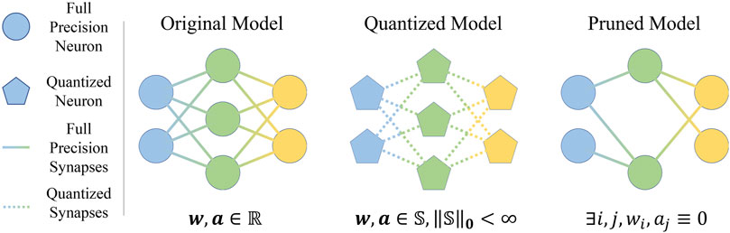
Figure 1. Comparison between the original, quantized and pruned models. $\mathit{w},\mathit{a}$ are weight, activation tensors respectively.

In addition to quantization and pruning, which facilitate the hardware implementation of CNNs, dedicated hardware accelerator designs can further improve energy and computation efficiency. The major motivation to develop specific neural network hardware comes from the memory bottleneck of the traditional von Neumann architectures (CPUs/GPUs), especially noticeable when deploying memory-dense applications, e.g., CNNs with millions of parameters. Specific hardware accelerators, e.g., FPGA-based (Umuroglu et al., 2017; Zhang et al., 2021), ASIC-based (Chang and Chang, 2019; Biswas and Chandrakasan, 2018) or In-memory computing (IMC) based (Sun et al., 2018b; Ankit et al., 2019) designs, help to address von Neumann bottleneck issues and deploy CNNs on low-power devices. Therefore, in this work, we try to provide a comprehensive review of specific hardware designs of quantized CNNs (QCNNs) and connect software-based QCNN methodologies with hardware deployment.

While previous studies have primarily reviewed neural network compression and quantization techniques from an algorithmic perspective (Neill, 2020; Guo, 2018; Qin et al., 2020; Kulkarni et al., 2022; Rokh et al., 2022; Gholami et al., 2021), they barely pay attention hardware implementations and often overlook the critical interplay between these algorithms and their hardware implementations. In contrast, our work bridges this gap by surveying both quantization algorithms and a wide range of QCNN-specific acceleration hardware. Furthermore, we offer insights into the challenges and open problems in QCNN hardware accelerator design, along with general guidelines for effective software-hardware co-design. Our main contributions are as follows:

• Integrated Review of Algorithms and Hardware: We survey various quantization techniques for CNNs alongside a detailed review of dedicated hardware accelerators—such as ASIC- and FPGA-based designs—that implement these methods. This dual perspective highlights how algorithmic choices impact hardware performance and vice versa.

• Guidelines for Software-Hardware Co-Design: We discuss practical strategies for co-designing quantization algorithms and hardware architectures. By outlining design trade-offs and optimization strategies, we provide a roadmap for developing CNN systems that maintain high performance under strict energy and resource constraints.

Both quantization algorithms, QCNN acceleration hardware design, and even network structure designs are rapidly evolving research topics. Hence, it is challenging to encompass an exhaustive survey of all relevant literature. The focus of this work is specifically narrowed to hardware accelerators for QCNNs that are tailored to maximize energy efficiency (e.g., ASIC- and FPGA-based designs), as opposed to those designed with an emphasis on scalability and peak performance. In alignment with this focus, the review of quantization algorithms and CNN models is mainly on those that are prevalently adopted by energy-efficient QCNN hardware accelerator designs. Given the defined scope of this paper, it is noteworthy that some cutting-edge CNN models (e.g., Vision Transformer + CNN(Guo et al., 2022), RegNet (Xu et al., 2022), DPN(Chen et al., 2017), Res2Net (Gao et al., 2019)), quantization techniques (e.g., codebook quantization, gradient quantization), and QCNN hardware platforms (e.g., GPUs, CPUs) will not be reviewed in extensive detail, as they are not common for energy-efficient on-edge processing. An overview illustrating the scope of this paper is provided in Figure 2. Nonetheless, we acknowledge and value the significant contributions of researchers in both fields who are missed by this work and extend our apologies to our readers for the inevitable limitations in coverage.

Figure 2

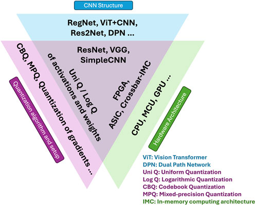
Figure 2. Overview of the scope of this work.

The remaining part of this paper is organized as follows. Section 2 introduces the basics of convention CNN and QCNN. Section 3 presents different quantization methods commonly used to quantize CNNs. In Section 4, different methods to generate a QNN are illustrated and benchmarked. In Section 5, various hardware accelerator designs are reviewed. Section 6 presents the future outlook on algorithms leading to more efficient QCNNs and corresponding hardware accelerator implementations. Section 7 concludes the paper.

2 Convolutional neural network

2.1 Full precision convolutional neural network

2.1.1 Convolution layer and fully connected layer

Inspired by the hierarchy model of the visual nervous system, Fukushima proposed the first neural network similar to modern-day convolution layers (Fukushima, 1980). LeCun et al. introduced the “LeNet-5” CNN in (LeCun et al., 1989; Lecun et al., 1998) for handwritten digit recognition systems, which is referred to as the first modern CNN trained with gradient-based backpropagation including all the essential building blocks in modern CNNs (convolution layers, pooling layers, and fully connected layers). Convolution layers are used to extract spatial features due to their spatial invariance.

Following the convolution layers, the fully connected layers are used to classify the abstracted features from the convolution layers and generate the final classification output.

2.1.2 Other auxiliary layers

In modern CNN architectures, additional auxiliary layers, including pooling, normalization, and dropout layers, are used along with the main convolution and fully connected layers. The pooling layers reduce the sizes of the convolution layers by sub-sampling the output feature maps with max/average operations.

As CNNs are becoming deeper and more complex, they also tend to be hard to be trained. To solve this problem, Ioffe et al. proposed the batch normalization technique in (Ioffe and Szegedy, 2015). Batch normalization normalizes the data over a mini-batch during training as ${\mathit{x}}_{BN}=\frac{\mathit{x}-\mu }{\sigma }\cdot \gamma +\beta$, where $\mathit{x},{\mathit{x}}_{BN}\in {\mathbb{R}}^{N_{\mathit{batch}}\times 1}$ are the data before and after batch normalization respectively, $N_{\mathit{batch}}$ is the batch size, $\mu ,\sigma$ are the mean and standard deviation of the inputs over the mini-batch. Two optional trainable parameters $\gamma ,\sigma$ are called affine parameters and involved in the final output computation enabling an affine transformation on the normalized data, restoring the representation capability of the neural network.

The other challenge in deep CNN training is overfitting. Srivastava et al. proposed the dropout technique in (Srivastava et al., 2014). By inserting dropout layers after convolution and fully connected layers, a certain portion of neurons is randomly chosen and dropped out during training, equivalent to training an ensemble of networks with different connections.

2.2 Typical convolutional neural networks

The design of CNNs has been widely explored recently. However, due to the limitation of IoT and edge devices, to the best of our knowledge, the latest CNN models like the RegNet family (Xu et al., 2022) and CNN-transformer hybrid architectures (Guo et al., 2022) are not implemented on dedicated hardware accelerators. Instead, only limited types of CNNs are referred to in the study of QCNNs. In this section, the commonly used CNNs in the study of hardware-related and mobile device-related QCNNs are introduced rather than the state-of-the-art CNN models.

2.2.1 LeNet-5

LeNet-5 (LeCun et al., 1989) is one of the earliest modern CNN architectures. It is designed for handwritten digit recognition with the Modified National Institute of Standards and Technology (MNIST) dataset. The structure of LeNet-5 can be shown in Figure 3a. It is often introduced in the studies as a case of light-weighted CNN.

Figure 3

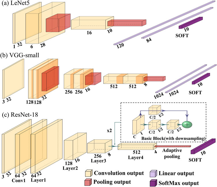
Figure 3. Network structure of (a) LeNet-5, (b) VGG-small, and (c) ResNet-18.

2.2.2 VGG family

Supported by GPU acceleration, CNNs have become deeper. One such network is AlexNet (Krizhevsky et al., 2017), which can support large datasets classification, e.g., Imagenet. AlexNet adapts a rectified-linear unit (ReLU) as the non-linear activation function. The other example of deep CNN is VGGNet, which achieves high accuracy using small convolution kernel sizes. Such deep networks contain up to a hundred million parameters overwhelming the edge/IoT-based implementations of these networks due to the limited memory and resources. Therefore, a simplified version of VGGNet, VGG-small (VGG-9), is designed for a smaller dataset (CIFAR-10) (Courbariaux et al., 2015). The structure of the VGG-small is shown in Figure 3b.

2.2.3 ResNet family

The challenges of deep neural networks with simply cascaded layers are vanishing or exploding gradient issues during the training. To address this issue, the ResNet CNN model was proposed, which is divided into small blocks (He et al., 2016). Each block consists of a few (usually 2 or 3) convolution layers, with an identity bypass connecting the input and output of the block to alleviate vanishing and exploding gradient problems. This allows the implementation of narrower but deeper networks, showing better performance than wider, shallower networks. Due to the modular design, the ResNet architecture can be scaled to up to a thousand layers. Figure 3c shows the network structure of a ResNet-18 modified for the CIFAR-10 dataset.

2.2.4 CNNs for mobile devices and TinyML

To achieve better power efficiency and lower inference latency on modern mobile devices, the complicated CNNs need to be redesigned. MobileNet (Howard et al., 2017) proposes a network design with depth-wise separable convolution layers (Sifre and Mallat, 2014). Compared with traditional convolution layers, the depth-wise separable convolution layers reduce both the number of computations and the number of parameters by $\frac{1}{C_{\mathit{out}}}+\frac{1}{k^2{C}_{in}}$ times. Additionally, most computations in the depth-wise separable convolution layers are contributed by the point-wise convolution with a kernel size of $1\times 1$, which can be executed by a highly optimized general matrix multiplication (GEMM) function. While for other convolution layers, the feature map needs to be rearranged in the memory before it can be processed by GEMM functions. To improve the performance further, the inverted bottleneck block requiring less computation compared with the traditional bottleneck block was introduced in MobileNetV2 (Sandler et al., 2018).

To scale up a CNN further, compound scaling factors are introduced in EfficientNet (Tan and Le, 2019). They scale up the width, depth, and resolution simultaneously leading to higher accuracy when more floating point operations (FLOPs) are allowed by the hardware setup. To generate a baseline CNN model with a certain target number of FLOPs, Neural Architecture Search (NAS) can be used. Then, a grid search can be performed with the generated baseline model to acquire the compound scaling factors for this model.

To further extend AI towards the edge, the concept of TinyML was proposed (Warden and Situnayake, 2019). TinyML includes hardware, software, and algorithms that enable on-device sensor data analysis on the edge. It also includes network structure design and optimization targeting low-power edge devices like microcontroller units (MCUs). Even though MobileNet and EfficientNet are optimized towards compactness, they still overwhelm the RAM size of typical MCUs. To overcome this memory bottleneck challenge, the MCUNet framework is proposed in (Lin J. et al., 2020). MCUNet adopts a two-stage NAS to generate an optimized model towards throughput and accuracy while meeting the memory constraint. The two-stage NAS is co-designed with a memory-efficient inference library supporting code generator-based compilation, model-adaptive memory scheduling, computation kernel specialization, and in-place depth-wise convolution. MCUNetV2 (Lin et al., 2021) introduces patch-by-patch inference scheduling in the inference library and receptive filed redistribution in NAS to further reduce peak memory consumption caused by the imbalanced memory distribution in CNNs.

2.3 Quantized convolutional neural network

To enable efficient deployment of CNNs on edge or IoT devices, CNNs need to be compressed. Various techniques have been developed for neural network compression, including pruning (Janowsky, 1989; Han et al., 2015; Guo et al., 2020), low-rank tensor approximation (Denton et al., 2014; Jaderberg et al., 2014), and quantization (Teng et al., 2019; Gong et al., 2014; Courbariaux et al., 2015; Hubara et al., 2017; Sun et al., 2020). In this work, we focus on quantization methods, which can be independently applied with other compression methods.

We summarize the achieved accuracies of various full-precision CNNs targeting different datasets in Figure 4. Due to the small memory size of MCUs and FPGAs, full-precision CNNs are too large to be deployed on such devices. To reduce the memory footprint, the parameters in the neural network can be quantized into a format with a shorter bit-width compared with the original 32-bit floating-point format. In (Gupta et al., 2015; Zhou et al., 2016; Rastegari et al., 2016), the authors quantize the weights of CNN into different bit-width formats achieving up to 32 times the size reduction with a cost of mild accuracy degradation. To reduce the issues of limited computation ability and power in IoT/edge devices, activation quantization has been proposed leading to more efficient computation kernels. For instance, when using binary quantization, multiply-accumulate (MAC) operations in a traditional full-precision neural network can be replaced by energy-efficient combination of XNOR and bit counting operation (Hubara et al., 2017; Rastegari et al., 2016; Zhou et al., 2016). Similar to weight quantization, accuracy degradation caused by quantization is acceptable.

Figure 4

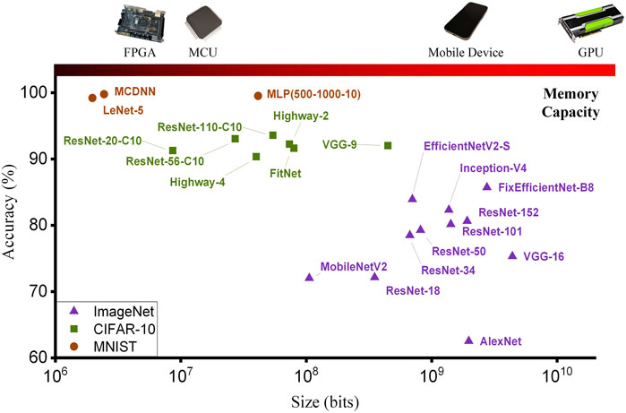
Figure 4. Comparison of convolutional neural network (CNN) model sizes against the memory capacities of various hardware platforms. For FPGA, memory capacity corresponds to on-chip block random access memory (BRAM), while standard random access memory (RAM) for other platforms.

Generally, QCNN is commonly referred to as a CNN with a quantized format of parameters (weights) and data flow (activations) to achieve a smaller network size and more efficient computation. Weights in CNN account for the majority of the size of the neural network. As the number of weights in the convolution and fully connected layers are in the order of $O(N^2)$, while the rest of the parameters (biases, affine parameters) are in the order of $O(N)$, with $N$ being the number of neurons in the layer. Hence, most of the published works focus on quantizing the weights of convolution layers and fully connected layers.

3 Quantization methods

Quantization maps a continuous interval into a set of discrete values. There are various mapping algorithms, which can be categorized into two subsets, deterministic quantization, and stochastic quantization. In deterministic quantization, the quantized value and original value have a one-to-one mapping. While the stochastically quantized value is sampled from a certain probability distribution parameterized by the original value. Sampling from a distribution requires more computation than a deterministic calculation. Additionally, gradient estimation is difficult with stochastic quantization leading to training complexity (Bengio, 2013). Hence, we focus on deterministic quantization algorithms.

3.1 Uniform quantization

Uniform quantization is the most commonly used quantization algorithm, which divides an interval into equal sub-intervals where all the data is represented by a single value. Each sub-interval corresponds to a set of linear uniformly distributed discrete values. Uniformly quantized value $w_q$ is represented as (Equation 1):

$\begin{array}{c}\hfill w_q=quant\left(w_c\right)=clamp\left(\lfloor \frac{w_c+b}{s}\rceil ,v_{\mathit{min}},v_{\mathit{max}}\right)\hfill \\ \hfill clamp\left(x,v_{\mathit{min}},v_{\mathit{max}}\right)=\left\{\begin{array}{c}{v}_{\mathit{min}}x\le v_{\mathit{min}}\hfill \\ x{v}_{\mathit{min}}<x<v_{\mathit{max}}\hfill \\ v_{\mathit{max}}x\ge v_{\mathit{max}}\hfill \end{array}\right.\hfill \end{array}(1)$

where $\lfloor .\rceil$ is a round function to the nearest integer, $w_c$, $b$, $s$ and $v_{\mathit{min}}$/$v_{\mathit{max}}$ are full-precision value, bias, scale factors and boundary values respectively. The simplest case of uniform quantization is binary quantization (with $b=0,s=\min (|x|),v_{\mathit{max}}=1,v_{\mathit{min}}=-1$) (Equation 2):

$w_q=quan{t}_2\left(w_c\right)=Sign\left(w_c\right)=\left\{\begin{array}{c}-1,w_c\le 0\hfill \\ 1,w_c>0\hfill \end{array}\right.(2)$

Another widely used uniform quantization is n-bits integer quantization (Equation 3):

$\begin{array}{c}\hfill w_q=quan{t}_k\left(w_c\right)=clamp\left(\lfloor w_c\rceil ,-2^{n-1},2^{n-1}-1\right)\hfill \end{array}(3)$

In practice, the full-precision parameter $w_c$ is passed through a bounded non-linear function before quantization. For instance, in (Hubara et al., 2017), a hard clip function is applied to the parameter to be quantized before actual quantization. In (Zhou et al., 2016), parameters are passed through a hyperbolic tangent function limiting the range of the parameters into the quantization range $[-\mathrm{1,1}]$. Therefore, the ability to update all the parameters is retained, even if the parameters are outside the quantization range. However, it is not always optimal to update all the parameters, this topic is detailed studied and discussed in (Sakr et al., 2022).

Generally, uniform quantization is simple, as all operations on the quantized parameters are either integer or bit-wise operations, suitable to be executed by arithmetic logic units (ALUs) in von Neumann systems, gate-level circuits in ASICs, and lookup tables (LUTs) in FPGA. However, uniform quantization inherently exhibits a poor dynamic range. With $n$-bit uniform quantization, the ratio $r$ between the largest positive value and the smallest positive value can be expressed as $r=\frac{2^{n-1}}{1}=2^{n-1}$. To mitigate this drawback, a full precision scale factor is attached to the quantized values (Zhou et al., 2016; Rastegari et al., 2016), at the cost of computation complexity. For instance, full precision scale factors are multiplied with corresponding quantized values and summed up during convolution operations, which requires full precision floating point arithmetic support on the hardware. Besides, other quantization methods have better dynamic range (discussed in the following section).

3.2 Low-precision floating point format and logarithmic quantization

One of the straightforward approaches to reduce data precision (reduce bit-width) while maintaining dynamic range is to truncate the commonly used IEEE-754 single-precision floating-point format to half-precision format. Examples of low-precision floating point formats are presented in Table 1. To further reduce the bit-width and computation complexity while maximizing the dynamic range, a 4-bit radix-4 logarithmic quantization algorithm (Sun et al., 2020) can be used in the format of $[\text{sign,\hspace{0.17em}exponent}]=[\mathrm{1,3}]$:

$\begin{array}{c}\hfill |w_q|=\left\{\begin{array}{c}{4}^{n-1},4^{n-1}\le |w_c|\le \frac{4^n+4^{n-1}}{2}\hfill \\ 4^n,\frac{4^n+4^{n-1}}{2}<|w_c|\le 4^n\hfill \end{array}\right.\hfill \\ \hfill n=-3,-2,-\mathrm{1,0,1,2,3}\hfill \\ \hfill sign\left(w_q\right)=sign\left(w_c\right)\hfill \end{array}(4)$

Derived from Equation 4, the ratio between the largest and smallest magnitude can be expressed as $r=\frac{4^3}{4^{-3}}=4^6$. Compared with 4-bit uniform quantization $(r=2^{4-1}=2^3)$, the logarithmic quantization has a much larger dynamic range $r$. This makes it suitable for the quantization of data with a large dynamic range, e.g., gradients. Neural network training with the 4-bit radix four logarithmic quantization can achieve comparable results as using a 32-bit floating-point format (Sun et al., 2020).

Table 1

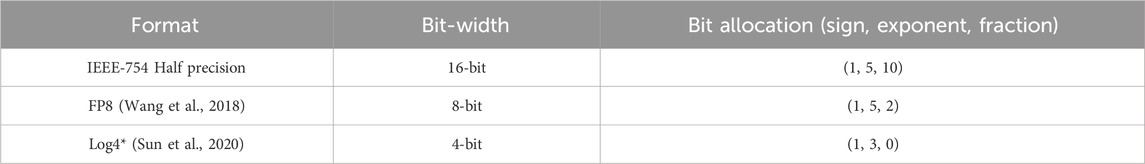
Table 1. Examples of different floating point format and logarithmic quantization format (* Log4 is a radix-4 format).

From the hardware point of view, the multiplication operation of logarithmically quantized data can be simply implemented with shift operations. However, the sum operation puts high requirements on accumulators due to the high dynamic range. Therefore, to support logarithmic quantization, the accumulator usually has large bit-width of the output or supports a floating point sum operation.

3.3 Codebook quantization

The parameters of a well-trained neural network follow a certain distribution, which is neither linear nor logarithmic. To represent these parameters, the quantized value set and corresponding mapping rules can be customized resulting in a codebook-style quantization. In (Gong et al., 2014), the quantized value set is found by k-mean clustering (Equation 5):

${\displaystyle \underset{c}{\min }}{\displaystyle \sum _i^N}{\displaystyle \sum _j^k}\Vert w_i-c_j{\Vert }_2^2,\mathbf{w}\in {\mathbb{R}}^{1\times N},\mathbf{c}\in {\mathbb{R}}^{1\times k}(5)$

Then, each value $c_j$ can be assigned an index to form a codebook. The index requires ${\log }_{2}k$ bits to be represented. With the quantized value set, the parameter can be quantized and represented using indexes, with $CB(x)$ being the inverse codebook mapping (value to index) (Equation 6):

$w_q=CB\left(\arg {\displaystyle \underset{c_j}{\min }}\Vert w_c-c_j{\Vert }_2^2\right)(6)$

A similar method is adopted and implemented on hardware in (Lee et al., 2017). In (Han et al., 2015), a network is quantized by codebook quantization using Equation 6 and finetuned. In (Teng et al., 2019), codebook quantization is applied, where the most frequent values form a quantization value set instead of the cluster centroids. The codebook is updated after every epoch during training. Uniform quantization and logarithmic quantization can be treated as a special case of codebook quantization with the quantized value showing uniform or logarithmic distribution.

The hardware requirements to implement codebook quantization depend on the values in the codebook. For instance, if these values are floating-point values, the hardware should support floating-point operations. Compared to uniform and logarithmic methods, codebook quantization brings additional overhead of reading the codebook.

3.4 Mixed-precision quantization

Different parts of the neural network tend to exhibit different levels of abstraction and expression ability (Chu et al., 2021). Hence, different quantization parameters can be chosen for different parts of the neural network to ensure optimum model size without accuracy degradation, which is named mixed-precision quantization (MPQ) (Rakka et al., 2022). MPQ can provide a full-precision accuracy while maintaining the same model size as extremely low bit-width quantization (Nguyen et al., 2020; Kim et al., 2020). In MPQ, quantization parameters (bit-width, scale factors, quantization boundaries, etc.) for different parts of the neural network can be determined by some specification/metrics of the corresponding part (Ma et al., 2021; Yao et al., 2021), by differentiable optimization (Li et al., 2020; Habi et al., 2020), or by reinforcement learning (Wang et al., 2020; Elthakeb et al., 2019).

MPQ implementation requires additional hardware support and creates hardware overhead to handle the heterogeneity brought by MPQ (Nguyen et al., 2020; Wu et al., 2021). Any quantization method, e.g., uniform, logarithmic or codebook, can be used to create a mixed-precision model.

4 How to generate a quantized neural network?

There are two main approaches to generate a quantized neural network (QNN) model: (1) quantizing a well-trained full-precision model, known as Post-Training Quantization (PTQ), and (2) training or fine-tuning the model with quantization effects incorporated, referred to as Quantization-Aware Training (QAT). PTQ is typically faster and more efficient in terms of runtime, energy consumption, and computation cost because it uses a small calibration dataset without modifying the model weights. However, PTQ often results in lower performance compared to QAT (Jiang et al., 2022; Gholami et al., 2021; Rokh et al., 2022). As discussed in subsequent sections, current edge-oriented hardware accelerators do not fully support neural network training. Consequently, in edge-oriented vision applications (where QCNNs are commonly deployed), models are usually prepared offsite—on servers where runtime, energy consumption, and computational cost are less critical—making the extra overhead of QAT acceptable in exchange for improved accuracyMenghani (2023). To fully exploit the advantages of PTQ, instead of applying it to edge-oriented vision tasks, PTQ is frequently employed in domains like large language models, where updating weights is prohibitively expensive even with modern computational resources Shen et al. (2024a). Given these considerations, we focus on QAT methods in this paper.

The major challenge for training QNNs is the stair-like nature of the quantization function, resulting in zero gradients. Therefore, traditional stochastic gradient descent (SGD)-based training methods cannot be applied directly for QNN training. Hence, the key challenge in QNN training is backpropagation methods. Based on the backpropagation of the loss, QNN training methods can be categorized into (1) approximated gradient methods with exact gradients and (2) exact gradient methods with gradual quantization (Figure 5).

Figure 5

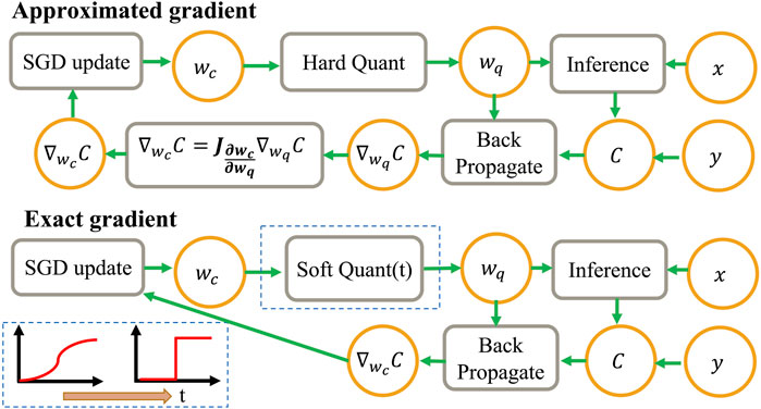
Figure 5. General training flow based on approximated gradient and exact gradient.

4.1 Approximated gradient under exact quantization

One of the solutions to the zero-gradient problem of the quantization function is to generate an approximated gradient to update the weights. The most straightforward approximation strategy is called the straight-through estimator (STE), which offers a simple and efficient way to backpropagate gradients through quantization functions. In STE, the Jacobian matrix ${\mathbf{J}}_{\frac{\partial {\mathbf{w}}_c}{\partial {\mathbf{w}}_q}}$ is set to be a diagonal matrix, where all diagonal entries equal to 1 (with $C$ being the cost) $\frac{\partial C}{\partial w_c}=\frac{\partial C}{\partial w_q}$. STE is used in all approximated gradient methods highlighted below.

4.1.1 Binary-connect and QNN

One of the first CNNs with binarized weights trained using STE is presented in (Courbariaux et al., 2015) (shown in Figure 6). This model achieved the accuracy comparable with floating-point models. Following the idea of training QNN using STE, this method is extended to n-bits uniform quantization of both weights and activations in (Hubara et al., 2017). In n-bit quantization (Hubara et al., 2017), the constraints are added to the weights and gradient values (a binary case example) (Equation 7):

$\begin{array}{c}\hfill w_c\left(t+1\right)=\text{clip}\left[w_c\left(t\right)-\eta {\nabla }_{w_c}C,-\mathrm{1,1}\right]\hfill \\ \hfill g_{a_c}=g_{a_q}\cdot {\mathbf{1}}_{|a_c|<1}\hfill \end{array}(7)$

where $g_{a_c}$, $g_{a_q}$ are gradients with respect to continuous activation and quantized activation, $\eta$ is the learning rate, and ${\mathbf{1}}_{|a_c|<1}$ equals to 1 when condition satisfied otherwise 0. Constraints on the weights and gradients of the activations avoid extremely large values, improving the training performance.

Figure 6

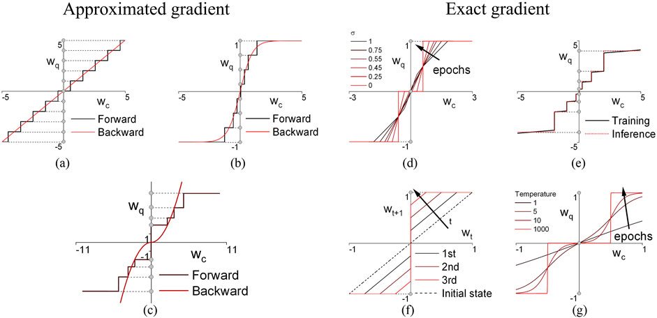
Figure 6. Visualization of weights before and after quantization during training using different training methods. (a) Basic STE. (b) DoReFa. (c) LNS-Madam. (d) ANA. (e) nBitQNN. (f) ProxQuant. (g) Sigmoid QN.

4.1.2 DoReFa-Net

In (Zhou et al., 2016), the method to quantize weights, activations, and gradients is presented (Figure 6) (Equation 8):

$\begin{array}{c}\hfill w_q=2quan{t}_{k,\mathrm{0,1}}\left(\frac{\tanh \left(w_c\right)}{2\max \left(|\tanh \left(w_c\right)|\right)}+\frac{1}{2}\right)-1\hfill \\ \hfill a_q=quan{t}_{k,\mathrm{0,1}}\left(\text{clip}\left(a_c,\mathrm{0,1}\right)\right)\hfill \\ \hfill g_q=2\max \left(|g_c|\right)\left[quan{t}_{k,\mathrm{0,1}}\left(\frac{g_c}{2\max \left(|g_c|\right)+\frac{1}{2}}\right)-\frac{1}{2}\right],\hfill \end{array}(8)$

where $quan{t}_{k,\mathrm{0,1}}$ is the k-bits uniform quantization function bounded between 0 and 1. The binary quantization case with $\mathbf{E}(|w_c|)$ being the mean of all the weights in the same layer can be formulated as:

$\begin{array}{c}\hfill w_b=\text{sign}\left(w_c\right)\cdot \mathbf{E}\left(|w_c|\right)\hfill \\ \hfill a_b=\text{sign}\left(a_c\right)\hfill \end{array}(9)$

As shown in Equation 9, a layer-wise scale factor $\mathbf{E}(|w_c|)$ is attached to the binarized weights. Therefore, the DoReFa-Net can not achieve a fully binarized inference. Similar to (Hubara et al., 2017), a hyperbolic tangent function and a clip function are applied to weights, and activations, respectively before quantization to avoid extremely large values and guarantee good performance. The first and last layers in the DoReFa-Net are not quantized.

4.1.3 LQ-Net

Even though Binary-Connect and Dorefa are based on uniform quantization, the data distribution of weights and activations in a well-trained neural network is non-uniform. In (Zhang et al., 2018), to reduce the quantization error, a quantized value is obtained as:

$w_q\in \left\{{\mathbf{b}}^{\mathbf{T}}\mathbf{v}|\mathbf{b}\in {\left\{-\mathrm{1,1}\right\}}^K\right\},(10)$

where $v$ is a vector representing the basis of the quantized value space, $b$ is a vector where all elements are either $-1$ or 1, and $K$ is the number of quantization bits. This method brings a more flexible quantized value space while being compatible with the bit-wise operation $({\mathbf{B}}_{\mathbf{w}}{\mathbf{B}}_{\mathbf{a}}^{\mathbf{T}})$:

${\mathbf{w}}_{\mathbf{q}}^{\mathbf{T}}\cdot {\mathbf{a}}_{\mathbf{q}}={\mathbf{v}}_{\mathbf{w}}^{\mathbf{T}}{\mathbf{B}}_{\mathbf{w}}{\mathbf{B}}_{\mathbf{a}}^{\mathbf{T}}{\mathbf{v}}_{\mathbf{a}}(11)$

Training using this method consists of optimization of the quantizer (vector $\mathbf{v}$ and $\mathbf{b}$) and optimization of the neural network parameters. Quantizer optimization is performed during the forward pass by minimizing the mean squared quantization error. For better efficiency, two vectors are optimized in a block coordinate descent fashion (two vectors are optimized alternatively). During the backward pass, neural network parameters are updated using the traditional SGD method with gradients passed through the quantizer via STE. To avoid adding considerably more parameters to the neural network, the learned quantizer is assigned channel-wise for weight and layer-wise for activations.

4.1.4 LNS-Madam

As logarithmic quantization offers a better dynamic range than uniform quantization, tailored logarithmic number system (LNS) with fractional exponents is proposed in (Zhao et al., 2022) and represented as (Equation 12):

$\begin{array}{c}\hfill x_q=\text{sign}\left(x_c\right)\cdot s\cdot 2^{\frac{\widehat{x}}{\gamma }}\hfill \\ \hfill \widehat{x}=\text{clip}\left(\text{round}\left({\text{log}}_2\left(\frac{|x_c|}{s}\right)\cdot \gamma \right),0,2^{b-1}-1\right)\hfill \end{array}(12)$

where $x_c$, $x_q$ are the value before and after quantization respectively, $\gamma$ is the base factor controls the quantization gap, $b$ is the quantization bit-width, and $s$ is a scale factor related to the magnitude of $x_c$. By selecting $\gamma$ from powers of 2, the overhead of hardware complexity is reduced while maintaining a variable quantization gap. In this LNS, the multiplication of the quantized values is easy to implement as the traditional power-of-2-based LNS. To efficiently perform add operations, the exponents are decomposed $\widehat{x}={\widehat{x}}_i+\frac{{\widehat{x}}_f}{\gamma }$, with $2^{{\widehat{x}}_i}$ being processed by lookup tables and $\frac{{\widehat{x}}_f}{\gamma }$ being processed by the approximation $2^{\frac{{\widehat{x}}_f}{\gamma }}\approx 1+\frac{{\widehat{x}}_f}{\gamma }$.

Low-precision LNS training framework based on a modified Madam optimizer presented in (Bernstein et al., 2020) directly optimizes the exponents in the LNS enabling 8-bit low-precision training. Figure 6 visualize the relation between quantized weight $w_q$ and original weight $w_c$ with $\gamma =2,b=3,s=2$.

4.1.5 PACT

In (Choi et al., 2018), the parameterized clipping activation (PACT) algorithm to quantize an activation to low bit-width without significant accuracy drop is proposed. One of the challenges of activation quantization is to decide the clipping range of a quantizer. A manual-designed clipping range is hard to adapt to different activation value distributions from various neural network architectures. An excessively small or large clipping range causes important values to be clipped or vanish in a quantization step size. PACT determines the clipping range automatically via gradient update (Equation 13):

$\begin{array}{c}\hfill \widehat{a}=Q_{\mathit{PACT}}\left(a_c\right)=\text{clip}\left(a_c,0,\alpha \right)\hfill \\ \hfill a_q=\text{round}\left(\frac{\widehat{a}}{\alpha }\cdot \left(2^k-1\right)\right)\cdot \frac{\alpha }{2^k-1}\hfill \\ \hfill \frac{\partial a_q}{\partial \alpha }={\mathbf{1}}_{a\ge \alpha }\hfill \end{array}(13)$

where $a_c$, $a_q$ are activation values before and after quantization, $\alpha$ is a learnable clipping range parameter and ${\mathbf{1}}_{a\ge \alpha }$ is 1 if $a\ge \alpha$ and 0 otherwise. PACT replaces the clipped values with $\alpha$ in the computation graph so that $\alpha$ can be automatically learned via gradients. PACT exhibits better accuracy over manually designed clipping ranges on various datasets.

4.1.6 Summary

The relations between the continuous and quantized versions of the weights for both forward and backward passes are visualized in Figure 6. Overall, approximated gradient based training methods approximate the gradient according to a “trend line” (red line in Figure 6). Also, these training methods execute the forward pass using quantized values, showing the potential of being deployed to low-end devices. However, most of the methods use full precision weights to aggregate the full precision gradients. The possibilities of training QNNs using low-precision latent weights (Banner et al., 2018; Gupta et al., 2015; Zhao et al., 2022) and gradients (Zhou et al., 2016; Rastegari et al., 2016; Sun et al., 2020) have been explored. Such methods make approximated gradient-based training methods to be good candidates for deployment on low-end devices.

4.2 Exact gradient with a gradual quantization

Besides approximated gradient methods, the other solution to the zero-gradient problem is a “soft” quantization using the time-evolving quantization function with non-zero derivatives, which converges to a “hard” quantization function as training proceeds.

4.2.1 Additive noise annealing (ANA)

In (Spallanzani et al., 2019), the expectations of quantized values and corresponding gradients are defined and derived considering a noise being added to the full-precision values. Consider $quant:\mathbb{R}\to \mathcal{Q}$ being a multi-step quantization function, $v$ being a zero-mean noise with probability density $\mu (-v)$:

$\begin{array}{c}\hfill w_q={\mathbb{E}}_{\mu }\left[quant\left(w_c+v\right)\right]=quant\left(w_c\right)\ast \mu \left(w_c\right)\hfill \\ \hfill \frac{\partial w_q}{\partial w_c}=\frac{\partial {\mathbb{E}}_{\mu }\left[quant\left(w_c+v\right)\right]}{\partial w_c}=quant\left(w_c\right)\ast \frac{\partial \mu \left(w_c\right)}{\partial w_c}\hfill \end{array}(14)$

where ${\mathbb{E}}_{\mu }$ is the expectation over $\mu$, and $(\ast )$ is the convolution operation. Equation 14 can be used to perform forward and backward passes of a noise-injected neural network. If $\mu (w_c)$ is a continuously differentiable function, the expectation ${\mathbb{E}}_{\mu }[quant(w_c+v)]$ of the quantization function with noise injected is not a multi-step function anymore, instead, a function with non-zero gradient, which can be expressed as $\frac{\partial w_q}{\partial w_c}$ in Equation 14. When the probability density function of the noise is a delta function $\mu (x)=\delta (x)$, the expectation ${\mathbb{E}}_{\mu }[quant(w_c+v)]=quant(w_c)$ matching the case of exact quantization. Hence, the key strategy of ANA is to construct a time-dependent noise probability density function $\mu (x,t)$, whose gradient is not always zero and converges to delta function as training proceeded: $\underset{t\to \infty }{\lim }\mu (x,t)=\delta (x)$. Practically, after a certain number of training steps, a hard quantization function is applied (i.e., no noise is injected), to generate QNN for inference.

Figure 6 shows an example of different expectations $w_q=\mathbb{E}[quant(w_c+v)]$ with different $\mu (-v)$ and $quant(x)$ being a ternary quantization function. $\mu (-v)$ is considered to be a uniform distribution $\mu (-v)\sim \mathcal{U}[-\sigma ,\sigma ]$. Large $\sigma$ at the beginning of the training results in a piece-wise linear function with non-zero gradients, enabling the backpropagation of the gradient through the quantization function. As training proceeds, $\sigma$ decreases towards zero, meanwhile, the expectation converges to a ternary quantization function.

4.2.2 ProxQuant

Unlike other methods, the ProxQuant algorithm (Bai et al., 2018) does not modify traditional SGD-based training, being directly compatible with SGD optimizers, e.g., Momentum SGD and Adam. The key point of the ProxQuant algorithm is adding a regularization process after each SGD update (Equation 15):

$\begin{array}{cc}\hfill w_{t+1}\hfill & \hfill ={\text{prox}}_{\lambda \cdot R}\left[w_t-\eta \nabla C\left(w_t\right)\right]\hfill \\ \hfill {\text{prox}}_{\lambda \cdot R}\left(x\right)\hfill & \hfill =\underset{\widehat{x}}{\mathrm{arg\; min}}\left[\frac{1}{2}\Vert \widehat{x}-x{\Vert }_2^2+\lambda \cdot R\left(\widehat{x}\right)\right]\hfill \end{array}(15)$

where $R(\widehat{x})$ is a regularizer, which achieves minimum value when $x\in Q$ with Q being a set containing quantized values. By applying $pro{x}_{\lambda \cdot R}(x)$ function, the weight is updated considering both SGD result and distance from the quantized set. The weights converge to the values in the quantized set $\mathcal{Q}$ after applying $pro{x}_{\lambda \cdot R}(x)$ several times. Figure 6 shows a special binary quantization (i.e., $\mathcal{Q}=-\mathrm{1,1}$) case when the weights are updated by appllying $pro{x}_{\lambda \cdot R}(x)$ for several times. The weight distribution gradually converges to the binary hard quantized case. To force the weights update towards the quantized set and to improve the performance, the parameter $\lambda =\lambda (t)$ can be increased as training proceeds.

Since the ${\text{prox}}_{\lambda \cdot R}[w_t-\eta \nabla C(w_t)]$ is applied iteratively, there is no closed form of the equivalent “Soft Quant” function shown in Figure 6. However, we can still use a generalized time-dependent “Soft Quant” function, which converges to a hard quantization function, to describe the effect of iteratively applying $pro{x}_{\lambda \cdot R}(x)$.

4.2.3 nBitQNN

In (Chen et al., 2020), a QNN training method that mixes the full precision weights and quantized weights to generate mixed-precision QNN is applied as (Equation 16):

$\begin{array}{c}\hfill w_q=\widetilde{quant}\left(w_c\right)=\alpha w_c+\left(1-\alpha \right)\widehat{w_q}\hfill \\ \hfill \widehat{w_q}=quan{t}_k\left(w_c\right)\hfill \\ \hfill \alpha \in \left(\mathrm{0,1}\right)\hfill \end{array}(16)$

where $\widetilde{quant}$ is a pseudo-quantization function mixing the full precision weight $w_c$ and the hard quantized weight $\widehat{w_q}$. $\frac{\partial w_q}{\partial w_c}=\alpha \ne 0$, enables the gradient to back propagate through $\widetilde{quant}(w_c)$. The parameter $\alpha$ adjusts the ratio between full precision weights and hard quantized weights. Under a sufficient number of training steps, the weights converge to the hard quantized values even though $\alpha$ is a finite constant. The radix-2 logarithmic quantization is used to hard quantize the weights, while the activations are not quantized.

4.2.4 Quantization using sigmoid and hyperbolic tangent

In (Yang et al., 2019), the quantization function reformulated using a combination of shifted and scaled step functions:

$w_q={\displaystyle \sum _{i=1}^n}{s}_i\mathbf{H}\left(\beta w_c-b_i\right)-o,(17)$

where $\mathbf{H}(x)$ is the standard unit step function, $s_i,b_i$ are the scale factor and shift of the corresponding unit step function, and $o=\frac{1}{2}{\sum }_{i=1}^n{s}_i$ is a global offset zero-centering the distribution of quantized parameter $w_q$. To overcome the zero-gradient problem of the step functions during training, the unit step functions in Equation 17 are replaced by temperature-modulated sigmoid functions $\mathbf{\sigma }(Tx)$:

$\begin{array}{c}\hfill w_q=\alpha \left[{\displaystyle \sum _{i=1}^n}{s}_i\mathbf{\sigma }\left(T\left(\beta w_c-b_i\right)\right)-o\right]\hfill \\ \hfill \mathbf{\sigma }\left(Tx\right)=\frac{1}{1+e^{-Tx}}\hfill \end{array}(18)$

where $\alpha$ is a layer-wise scale factor for the output. With Equation 18 being a differentiable function, the gradient can be backpropagated through the neural network. As the training proceeds, the temperature $T$ grows, reducing the gap between $\mathbf{\sigma }(Tx)$ and unit step functions (Figure 6). Once the training is finished, the unit step functions are used in inference and validation. To guarantee high accuracy, training is divided into three phases: training a full precision neural network, training with weight quantization only, and training with activation quantization while fixing weight quantization.

In (Gong et al., 2019), the differentiable soft quantization framework (DSQ) is proposed, which shares a similar idea of quantizing data piece-wisely using a series of evolving hyperbolic tangent basis functions. Different from (Yang et al., 2019), the evolution of the basis functions is not performed explicitly with the training progress. A characteristic variable (describing the error between hard quantization and basis functions) is calculated and minimized during training. Additionally, DSQ adopts trainable clipping ranges similar to PACT (Choi et al., 2018).

4.2.5 Summary

Exact gradient methods adopt evolving quantization functions to guarantee a feasible gradient during training and reach hard quantization at the end of training. However, this implies that these methods need to be operated with full precision data. Hence, they are more suitable for a cloud-based execution generating QNNs to be deployed on edge devices.

4.3 Fake and real quantization

Most quantization studies implement their algorithms in software (e.g., using Pytorch, Tensorflow) (Li et al., 2021). Therefore, all the quantization operations and quantized data are simulated in floating-point format, which can be referred to as “Fake Quantization”. On the contrary, when the quantized models are deployed on hardware, the quantized data is processed by executors supporting the corresponding format (e.g., 8-bit integer arithmetic unit for 8-bit uniform quantization). This can be referred to as “Real Quantization”. The data format mismatch between fake and real quantization may cause unavoidable data value differences. Adaption from fake quantization to real quantization considering different hardware architectures is discussed in Section 5.

4.4 Benchmarking

In this section, the training methods mentioned in Section 4 are benchmarked under different configurations using corresponding open-source codes modified where required.

4.4.1 Network and training configurations

In the aforementioned works, different configurations of either the network or training are used. In all the original works, the affine operation of the batch-norm layer is enabled and all the trainable parameters for affine operation are not quantized. While in our experiments the affine operation is only enabled according to configurations. Affine operation adds two full precision trainable parameters at each output channel. They do not affect the performance during inference with batch normalization fusing, however, during training they degrade the compression rate and increase the computation complexity. To improve generalization ability, all the aforementioned methods involve data augmentation. To analyze the influence of each setting, we benchmark the aforementioned training methods using the settings summarized in Table 2.

Table 2

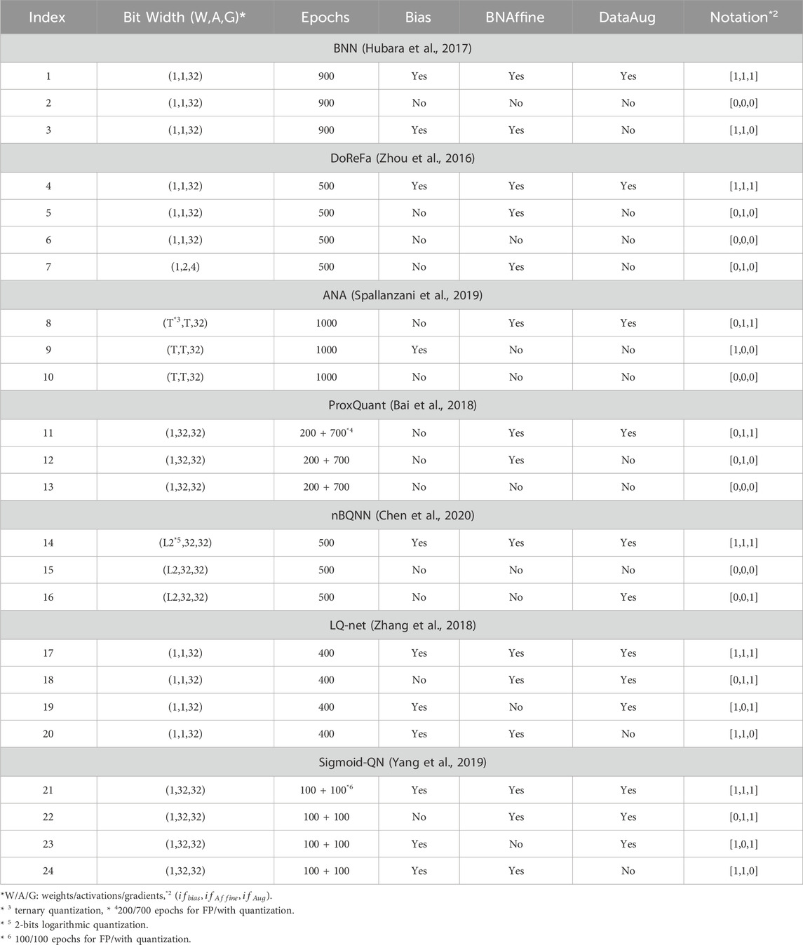
Table 2. Benchmark settings for training methods.

4.4.2 Experiments

The dataset and neural network structure adopted in the experiments are CIFAR-10 and VGG-small, respectively. We prioritize the official code provided by the authors during the benchmark and keep a minimum modification. For a fair comparison, the data augmentation conducted in the experiments only includes random cropping and random horizontal flipping. The number of training epochs is chosen to be large enough for each case to be well-trained.

The results of different cases are visualized in Figure 7. To compare the relative size of the networks in different cases, we calculate the averaged bit-width using the following equation (Equation 19):

$B{W}_{\mathit{Avg}}=\frac{{\sum }_l{\sum }_{i,w_i\in l}B{W}_{w_i}}{N_{1b,\left[\mathrm{0,0,0}\right]}},(19)$

where $B{W}_{w_i}$ is the bit-width of weights $w_i$ in layer $l$ and $N_{1b,[\mathrm{0,0,0}]}$ is the number of trainable parameters in the 1-bit QNN without bias and batch normalization affine parameters.

Figure 7

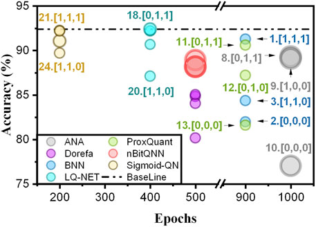
Figure 7. Visualization of the benchmark results, with important cases marked using “Index” and “Notation” in Table 2. The circle diameter represents the size of the model.

Overall, all the methods can achieve an accuracy higher than 85$\%$. The BNN (Hubara et al., 2017), ProxQuant (Bai et al., 2018), LQ-net (Zhang et al., 2018) and Sigmoid-QN (Yang et al., 2019) methods result in accuracy over 90$\%$, close to the full precision model baseline (Lee et al., 2016). DoReFa and nBitQNN methods are more robust against different bias and affine operation settings. DoReFa introduces scale factors to each layer, and nBitQNN uses logarithmic quantization, which brings them extra representation abilities. ANA, DoReFa, and nBitQNN are not sensitive to the presence of data augmentation. The BNN method is more vulnerable to the absence of data augmentation. Comparing Case 1 and Case 3 (Table 2), the BNN method experiences an accuracy drop of 6.92% when data augmentation is removed.

An average bit-width is represented by the diameter of the circles in Figure 7, which shows that the additional parameters from the biases and affine operations occupy a small portion of the network size. Even though shift-based batch normalization is introduced in (Hubara et al., 2017) and realized in (Zhijie et al., 2020), batch normalization still brings overhead during training.

LQ-net and Sigmoid-QN achieve the best accuracy close to the full precision baseline model at the cost of additional scale factors and the first and the last layers are not quantized. The BNN method can achieve an accuracy of over 90% while maintaining the size of a binary neural network with all the layers quantized without scale factors. However, it is sensitive to bias and batch normalization parameters. ProxQuant and nBitQNN also achieve high accuracy, but they do not quantize the activations. The ANA method also demonstrates high accuracy but has a larger model size and is sensitive to changes. DoReFa is robust against configuration changes and supports gradient quantization. However, the first and last layers are not quantized in DoReFa, and layer-wise scaling factors are adopted bringing overhead in terms of compression rate and computation complexity.

4.5 Strategies to improve QNN performance

This section introduces general strategies helping to improve the performance of QNN, including learning rate scheduling and trade-offs between accuracy and model complexity.

4.5.1 Learning rate scheduling

For QNNs, the selection of learning rate is more critical than full precision networks. A low learning rate leads to slow convergence, while a high learning rate causes an unstable weight update. Figure 8 shows the gradient descent process for both full precision and quantized networks. In full precision models, the loss surface is smooth, the gradients shrink down as the loss approaches the minima (Figure 8a). In QNNs, the loss surface is stair-liked. If the gradients are calculated and referred to as the quantized value (methods using approximated gradients in Section 4.1), the gradient preserves a constant value regardless of the current position on the flat plateau of the loss surface, causing a cross over the minimum (Figure 8b). Hence, without gradient shrinking down as in the full precision case, the training of QNNs must be performed with lower learning rates compared with a full precision case. This phenomenon is confirmed by experiments in (Tang et al., 2017).

Figure 8

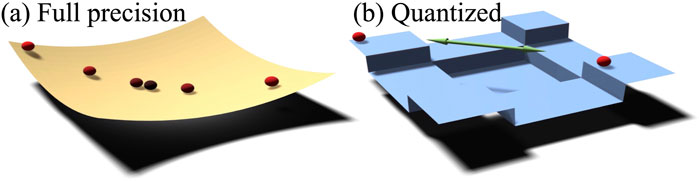
Figure 8. Gradient descent process for (a) full precision and (b) quantized neural networks.

QNN training usually starts with lower learning rates compared to full-precision networks. For instance, the learning rate for training full precision VGG network in (Simonyan and Zisserman, 2014) starts at $10^{-1}$, while for training a small VGG network for CIFAR-10 dataset in (Hubara et al., 2017) starts at $5\times 10^{-3}$. Besides the difference in the starting learning rates, different learning scheduling methods are adopted for QNN training, including exponential decaying (Courbariaux et al., 2015; Hubara et al., 2017; Spallanzani et al., 2019; Chen et al., 2020), and manual assigning (Bai et al., 2018; Zhou et al., 2016).

4.5.2 Trade for a higher accuracy

The majority of QNN training methods are offline methods, which can be performed on high-performance computation platforms, e.g., cloud servers. Meanwhile, some QNN applications are not strictly constrained by computation power or computation time. Hence, there are some strategies to increase the QNN accuracy at the cost of computation complexity or computation time.

The easiest way to improve accuracy without increasing a model size is to increase activation precision. For example, if the same network is trained with the DoReFa-Net method, a model trained with 2-bit activations achieves the accuracy of 86.5$\%$ with SVHN dataset (Netzer et al., 2011), while the model with 1-bit activations results in 84.1$\%$ accuracy. In (Tang et al., 2017), instead of directly increasing activation precision, multiple-quantization of the activations is performed. This method is more suitable for CPU/GPU-based computation platforms, while directly increasing the number of bits is more preferred by FPGA/ASIC-based platforms. In (Liu et al., 2018), a full precision bypass is introduced in each layer. The activation of $l$-th layer in this architecture can be expressed as (Equation 20):

${\mathbf{a}}^l=AF\left({\mathbf{z}}^l+{\mathbf{z}}^{l-1}\right)=AF\left[L\left({\mathbf{W}}^l,{\mathbf{z}}^{l-1}\right)+{\mathbf{z}}^{l-1}\right],(20)$

where ${\mathbf{z}}^l$ and ${\mathbf{a}}^l$ are the layer outputs before and after the quantization and activation, $AF()$ represents quantization and activation function, and $L$ is the operation the layer performs parameterized by ${\mathbf{W}}^l$. By introducing the bypass, a binary ResNet-34 network can achieve a top-1 accuracy of 69.7$\%$, showing an accuracy boost compared with the case without the bypass (67.9$\%$).

In (Tang et al., 2017), a new regularization term substituting commonly-used L2 norm regularization is proposed. In binary QNN, the ideal quantized parameters take the values of {-1, 1}. However, the traditional L2 norm regularization term forces the parameters to approach zero, which contradicts the distribution of the parameters in a binarized network, resulting in frequent weight fluctuation during training. Hence, new regularization biases the update of parameters toward their designated quantized value (e.g., in binary quantization case, the parameters are biased toward $-\mathrm{1,1}$) The new object function for QNN training using the proposed regularization term in binary quantization case can be expressed (Equation 21):

$J\left(\mathbf{W}\right)=\mathbb{L}\left(\mathbf{W}\right)+\lambda {\displaystyle \sum _{l=0}^L}{\displaystyle \sum _{d=0}^D}\left[1-{\left(W_{l,d}\right)}^2\right],(21)$

where $\mathbb{L}(\mathbf{W})$, ${\sum }_{l=0}^L{\sum }_{d=0}^D[1-{(W_{l,d})}^2]$, $\lambda$ are the loss term, regularization term, and trade-off hyperparameter respectively.

The other QNN training strategies, including two-stage optimization (TS), progressive quantization (PQ), and guided training, are shown in (Zhuang et al., 2018). TS consists of two steps: (1) weight quantization during training, and (2) activation quantization with trained weights. TS helps to avoid local minima when training a network from scratch. Moreover, instead of quantizing directly to the fixed bit-width (e.g., 2 bits), the network is quantized progressively (e.g., 32-bits$\to$16-bits … 2-bits) with the parameter in the higher precision model being the initial value for the lower precision model training. This guided training refers to QNN training using guidance loss from a teacher model, which shares the same structure as the quantized model. More specifically, at the output of each layer in the quantized model, the loss from the label (back propagated from the network output) is combined with the loss between the full precision and quantized model at the same position. This is called layer-wise knowledge distillation (Hinton et al., 2015; Heo et al., 2019; Leroux et al., 2020). With the proposed set of training strategies, the accuracy of the trained 4-bits AlexNet (Krizhevsky et al., 2017) outperforms the same network trained using DoReFa-Net (Zhou et al., 2016) by 2.8$\%$.

The other method to improve QNN accuracy is relaxing the compression rate if the application is not strictly constrained by memory size. In (Chu et al., 2021), mixed-precision QNN is proposed. As the features propagate along the network, they become more abstract and separable. Therefore, each layer of QNN can be quantized using a set of decreasing bit-widths as the layer goes downstream. For example, VGG-7 is quantized using {8-4-2-1-1-1}-bits for each layer from the input to the output, respectively. For the CIFAR-10 dataset, this network shows an accuracy of 93.22$\%$, while the full-precision model achieves an accuracy of 92.48$\%$. Also, the size of such QNN is 1.06 times the size of the binarized network.

In (Sakr et al., 2022), tensor clipping during QNN training is considered. Commonly, the tensor values are scaled based on the maximum in this tensor; however such scaling results in a large quantization step (especially for uniform quantization). As most of the tensor values are small, maximum scaling makes quantization bit-insufficient. In (Sakr et al., 2022), an algorithm to determine the optimal clipping and scaling factor for each tensor during each iteration of neural network training is shown. The optimal clipping factor minimizes the overall mean squared error including quantization error and clipped error.

For conventional quantization-aware training methods, it is common to use STE for gradient estimation. However, STE can cause gradient explosion by assigning clipped values with constant gradients. Though assigning zero gradients to the clipped values can avoid such explosion, the clipped values are prevented from being trained equivalent to shrink model size. To mitigate these two challenges, a magnitude-based gradient estimator, which assigns smaller gradients to the clipped values away from the threshold, is proposed in (Sakr et al., 2022). By applying both the optimal clipping values and gradient estimator, $<1\%$ accuracy degradation on the ImageNet dataset using 4-bit quantization compared to the full precision model is achieved in (Sakr et al., 2022).

5 Hardware implementation of QNNs

Efficient hardware implementation of a deep neural network for low-resource hardware requires compression techniques, including quantization, pruning, and Huffman coding (Chen et al., 2020). Usually, reduction of energy consumption, memory access, and data transfers between memory and computation units is achieved by simplifying computationally complex operations, e.g., floating-point computations. In this section, we discuss three main types of QNN implementations: FPGA-based solutions, ASIC solutions, and emerging non-volatile memory (NVM) based CNN implementations. This review focuses on state-of-the-art works considering the studies from the last 5 years with systematic neural network evaluations on hardware.

In QNN hardware, different quantization schemes require different bit configurations (Ryu et al., 2020). QNN hardware can be divided into 3 main groups based on the quantization scheme: (1) fixed-point arithmetic, (2) power-of-two quantization (logarithmic quantization), and (3) binary representation. Compared to the floating-point representation, fixed-point arithmetic keeps the location of the radix point fixed (Figure 9a). The power-of-two scheme represents the weights in the form of $2^i$, which allows replacing computationally expensive multipliers with a shift operation. In binary representation, 1-bit weights and activations are used; however, most of the implemented binary hardware still requires multi-bit support for the input layer and weight update (Hashemi et al., 2017). Compared to floating-point operations, QNNs improve energy efficiency significantly. For example, the 4-bit fixed-point representation and binarized neural networks allow for more than 90% of power savings compared to the 32-bit floating-point representation of weights.

Figure 9

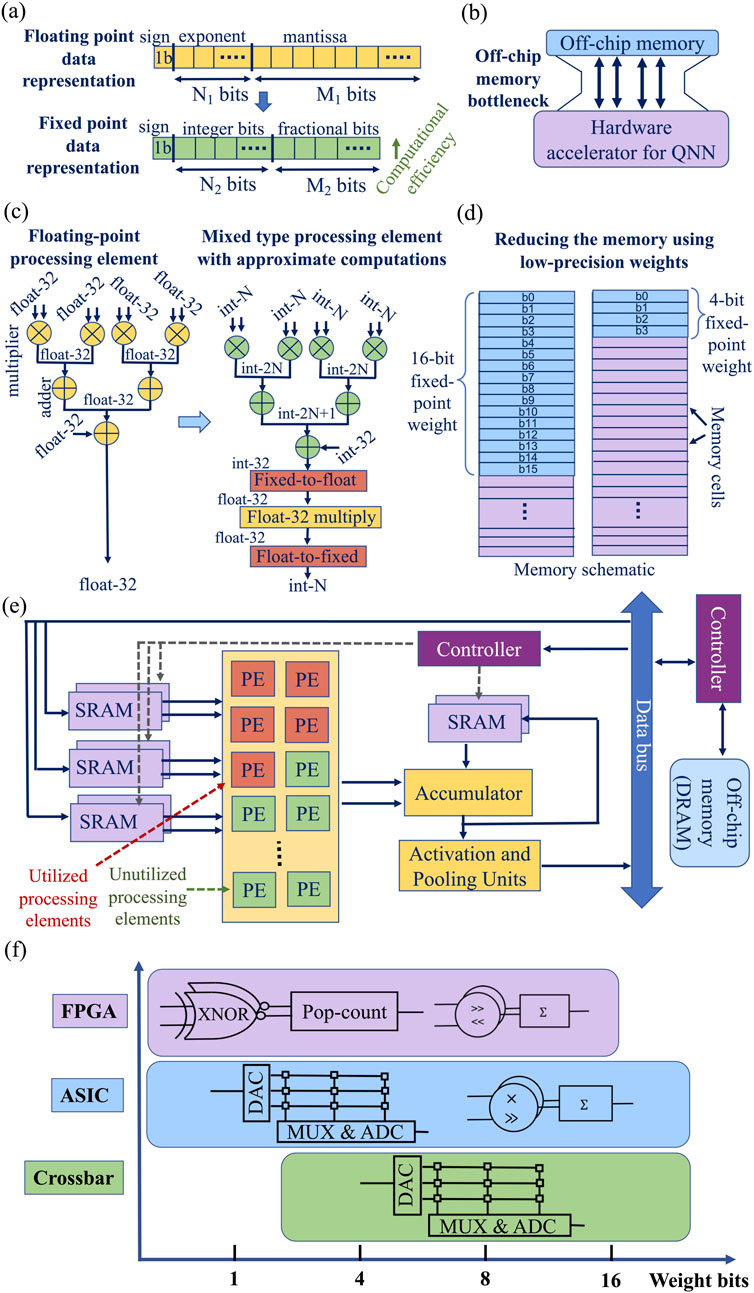
Figure 9. (a) Floating-point versus fixed-point operations. (b) Off-chip memory bottleneck. (c) An example of moving from floating point operations to approximate operations in a processing element (Wei et al., 2019). (d) Reducing the memory space with low-precision computation. (e) Example of QNN accelerator (PE-processing element), modified from (Chang and Chang, 2019). (f) PE preference for different hardware architecture under different bit-width.

QNN hardware accelerators focus on different issues affecting hardware efficiency, including data movement, hardware efficiency, memory consumption, and hardware utilization.

Similar to any neural network hardware design, one of the main challenges of QNN hardware is data movement between the QNN accelerator and off-chip memory storing QNN weights (Figure 9b). Typically, data movement is more energy-consuming than computation (Chen et al., 2016). This problem is targeted by in-memory computing-based QNN accelerators (Krestinskaya et al., 2023). The other challenge is to improve the energy efficiency of QNN hardware while preserving the performance accuracy. This can be addressed by combining fixed-point approximate operations with floating-point operations to create mixed-type processing elements (Figure 9c) (Wei et al., 2019). Memory consumption problem is tackled by lowering data (weights) precision (Figure 9d) (Wei et al., 2019). Various data reuse strategies are explored to improve memory efficiency (Ankit et al., 2019; Yao et al., 2020; Song et al., 2017; Shafiee et al., 2016). Hardware efficiency often comes with the cost of hardware utilization, when some processing elements (PEs) remain unused (Figure 9e). Data utilization, data flow complexity, and resource allocation along with resource parallelisms should be considered in any QNN design, especially for FPGA-based QNNs (Chang and Chang, 2019). Different processing engine designs are summarized in Figure 9f. For FPGA-based accelerators, the “on-chip” part only refers to the parallel acceleration parts implemented on FPGA fabrics. For some FPGA accelerator designs, the host CPU is either implemented using on-chip ARM processors or directly synthesized using resources on FPGA fabrics.

The other challenge of translating QNN to hardware implementation is relate to algorithm-hardware co-design challenges (Zhang et al., 2021). This involves finding the trade-offs between performance accuracy and hardware cost. The transition from software design of QNN to hardware implementation involves loops unrolling in a software algorithm, mapping software computations to particulate hardware blocks, array partitioning, matrix decomposition, loop pipelining, etc. In addition, it is also important to accommodate the quantization and processing differences in different types of layers. For example, convolution layers are computational-centric (few parameters requiring many computations), while fully connected layers are memory-centric (many parameters used once requiring loading from external memory in some cases contributing to the hardware efficiency limitations) (Qiu et al., 2016). The other challenge is to accommodate layer-wise and mixed-precision quantization implemented in software into the hardware, which varies from one QNN design to the other.

This section focuses on QNN architectures implemented on FPGA and ASIC, and related open challenges. Also, designs with emerging non-volatile memory devices are considered. Table 3 shows the summary of QNN hardware architectures. Figure 9 illustrates the area and power efficiency of different QNN architectures with respect to the precision of weights. The performance of RRAM-based architectures and SRAM-based ASIC implementations of QNNs are comparable in terms of power efficiency, while FPGA-based designs compromise energy efficiency due to hardware reconfigurability. This section also provides general guidelines on software-hardware co-design of QNN accelerators.

Table 3

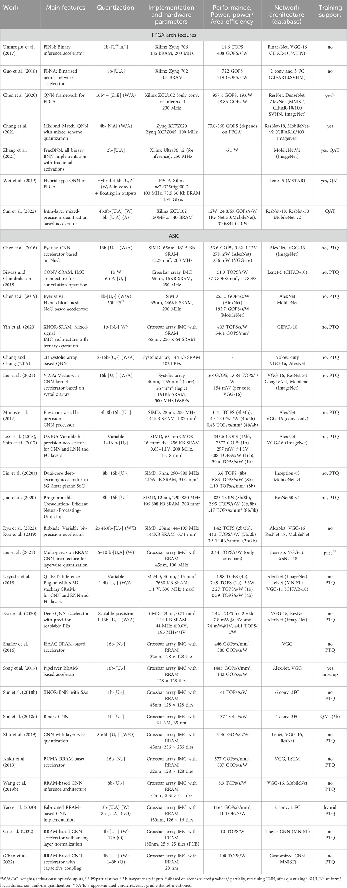
Table 3. Summary of QNN hardware.

5.1 FPGA-based implementations of QNNs

Field Programmable Gate Arrays (FPGAs) are designed for fixed point computations implemented using lookup tables (LUTs). Even though floating-point computation is possible to implement on FPGA using Digital Signal Processing (DSP) blocks, this is expensive and inefficient. To convert a QNN design into FPGA-based hardware implementation, different frameworks can be created to automate such conversion (Umuroglu et al., 2017; 2020). For example, LogicNets framework converts trained QNNs into equivalent netlists of truth tables for FPGA including network sparsity exploration to reduce neuron fan-in (Umuroglu et al., 2020). Fan-in reduction contributes to efficient LUT-based QNN implementations on FPGA.

5.1.1 Binarized and multi-bit precision neural networks on FPGA

Binarized Neural Networks (BNNs) are the most resource-efficient QNN designs on FPGA (Figure 10) (Umuroglu et al., 2017; Guo et al., 2018; Zhang et al., 2021; Qin et al., 2020). One of the most well-known BNN accelerators on FPGA is FINN (Umuroglu et al., 2017), which automatically converts Theano-trained BNN to synthesizable C++ description with optimized hardware blocks to synthesize a bitfile through High-Level Synthesis (HLS) software to deploy to FPGA. The binarization of neural network weights reduces memory consumption and improves computation speed. Typically, the input layer of BNN is not binarized to preserve input features and accuracy. To binarize the input layer in BNN, binary padding can be used to provide resource parallelism and scalability for FPGA-based implementations, as in (Guo et al., 2018; Zhang et al., 2021).

Figure 10

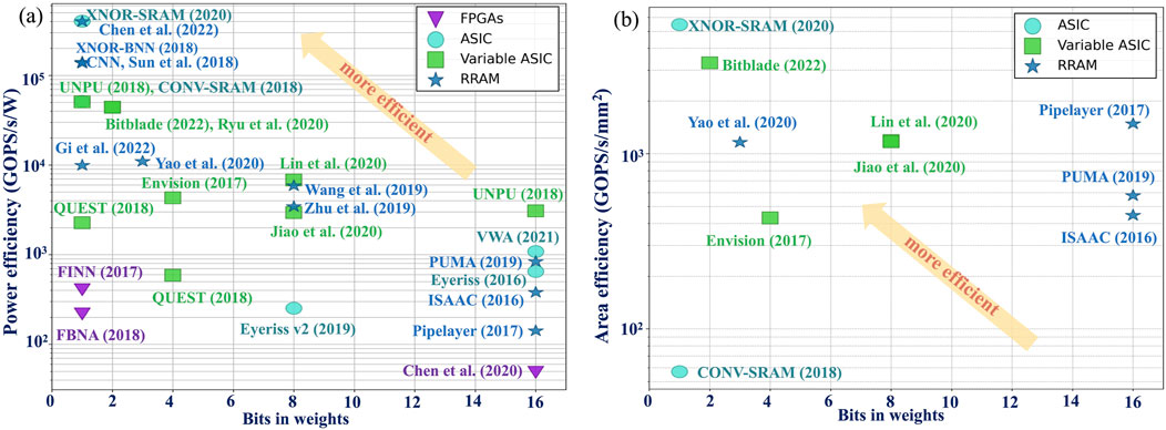
Figure 10. Power (a) and area (b) efficiency of QNN hardware implementations with respect to weight precision.

Maintaining high accuracy after binarization is one of the main challenges of BNN, which requires specific training methods. Real-to-Binary Net framework proposed in (Martinez et al., 2020) performs progressive teacher-student training. Starting with a full-precision teacher model and a student model with soft-binarized activations (using $tanh$ function), the student model is trained with additional guidance from the teacher model. In the following steps, the student model from the previous step becomes the teacher model in the current step, and the activations and weights of the new student model are progressively quantized in each step. By performing progressive teacher-student training, the resulting BNN experiences less accuracy degradation. The other method to preserve BNN accuracy is precision gating, where the important features are computed using higher precision. In FracBNN (Zhang et al., 2021), a dual-precision activation quantization is implemented where activations are quantized with either 1-bit or 2-bit based on their contribution to network accuracy (determined by a trainable parameter). An additional sparse binary convolution for the additional bit is performed for those critical activations that need to be quantized with 2 bits.

There have been several multi-bit FPGA-based implementations of QNN proposed recently (Ding et al., 2019; Hu et al., 2022; Chen et al., 2020). One of the most common quantized weights representations used for FPGA-based QNNs is the power-of-two method quantization method, as in FlightNN (Ding et al., 2019). To improve hardware efficiency further, the multiplication operations can be replaced by a lightweight shift operation (Ding et al., 2019) or be approximated by a different number of shift-and-add operations (Chen et al., 2020). To improve QNN efficiency further, the design of DSP blocks for quantized MAC operations can be optimized (Hu et al., 2022).

5.1.2 Mixed-precision and hybrid neural networks on FPGA

Mixed-precision and hybrid QNN designs require additional design considerations for efficient implementation. Inconsistent precision throughout the neural network layers can affect the utilization of heterogeneous FPGA hardware resources (Chang et al., 2021). In the Mix-and-Match FPGA-based QNN optimization framework (Chang et al., 2021), this problem is avoided using mixed quantization, combining sum-of-power-of-2 (SP2) and fixed-point quantization schemes for different rows of weight matrix due to different distribution of weights in different rows. The quantization scheme can also be adjusted for the distribution of the weights. For example, the Mix-and-Match framework uses the quantization scheme suitable for Gaussian-like weight distribution, where multiplication arithmetic is replaced with logic shifters and adders that can be implemented on FPGA using LUTs.

Hybrid quantization can also be used to improve QNN accuracy and efficiency in FPGA-based implementations. For example, in hybrid-type inference in (Wei et al., 2019), both convolution kernels (feature maps) and parameters are quantized to a signed integer, while integer/floating mixed calculations are used for the outputs. In the inference phase, the weights and activations in convolution layers are quantized, while the dot product output is de-quantized and represented as a 32-bit floating-point number before batch-normalization operation. The floating-point batch normalization output is fetched to the activation function, and the activation function output is quantized to integer representation. This helps to reduce the number of LUTs, flip-flops, DSP blocks, and BRAM blocks in the design.

Mixed-precision can also be used for intra-layer quantization. In (Sun et al., 2022), a mixed-precision algorithm combines a majority of low-precision weights, e.g., 4 bits, with a minority of high-precision weights, e.g., 8 bits, within a layer. The weights leading to high quantization errors are assigned to be of high precision. Moreover, in (Sun et al., 2022), quantization optimization techniques, including DSP packing, weight reordering, and data packing, are used.

5.2 ASIC implementations of QNNs

ASIC implementations of QNNs can be broadly categorized into conventional digital and mixed-signal designs, such as systolic arrays (Chang and Chang, 2019; Liu et al., 2021) or single/multiple instruction multiple data (S/MIMD)-based architectures with multiple cores (Lee et al., 2018; Shin et al., 2017), as well as designs leveraging emerging technologies like In-memory computing (IMC) (Krestinskaya et al., 2022; 2024a) and neuromorphic computing (Shen G. et al., 2024; Matinizadeh et al., 2024). Among these emerging technologies, SRAM- and RRAM-based IMC implementations have advanced the most, therefore, this work primarily focuses on them. The key distinction between IMC-based designs and traditional von Neumann architectures, where memory and processing units are separate, is that computation occurs directly within the memory. IMC designs can be based on either volatile (SRAMs and DRAMs) or non-volatile memory devices, e.g., resistive random-access memory devices (RRAMs), phase-change memory devices (PCM or PCRAM), etc (Krestinskaya et al., 2023).

5.2.1 Fixed-precision ASIC implementations of QNN

Based on Figure 9, ASIC implementations of QNNs are more efficient than FPGA-based implementations, as they are usually hardwired in an optimum way and cannot be reconfigured. Same as FPGA-based designs, ASIC-based implementations also use a shift operator instead of the multipliers via power-of-two quantization to improve energy efficiency. The multiplication can also be converted to two shift operations and one addition, as in LightNN (Ding et al., 2017; Ding et al., 2018). Also, approximate multiplication can be used, which drops the least significant powers of two limiting the number of shifts and adds (Ding et al., 2018). Some ASIC accelerator designs retain a certain level of flexibility (Moon et al., 2022; Lee S. K. et al., 2021). In (Moon et al., 2022), a framework supporting from 1 to 4-bit of arbitrary base quantization (Park et al., 2017) is proposed. For arbitrary base quantization, hardware blocks performing sorting, grouping, and population counting are adopted. In (Lee S. K. et al., 2021), an accelerator supporting both 8/16-bit floating point format and 2/4-bit integer format, where data pipelines for these formats are separated and implemented in dedicated hardware, is proposed. This accelerator supports both training and inference using floating point and integer data correspondingly.

The hardware efficiency of QNN accelerators is affected by architecture hierarchy, organization of processing elements (PEs), network-on-chip (NoC) structure, and the type of NoC. For example, Eyeriss is the other accelerator using 16-bit fixed-point computation, where data movement and DRAM access are reduced by reusing data locally (Chen et al., 2016). The improved version of Eyeriss, Eyeriss v2 (Chen et al., 2019), has a hierarchical mesh NoC with sparse PE architecture adaptable to the different amounts of data reuse and bandwidth requirements aiming to improve resource utilization.

CONV-SRAM (Biswas and Chandrakasan, 2018) and XNOR-SRAM (Yin et al., 2020) architectures are the other ASIC QNN accelerators to improve energy efficiency and reduce the number of computations. In (Yin et al., 2020), binary weights and ternary data representation [-1,0,1] for XNOR-and-accumulate operation are used. To improve computation speed and reduce memory access, systolic array-based CNN implementation can be used (Chang and Chang, 2019; Liu et al., 2021). In (Chang and Chang, 2019), a systolic array-based CNN, VWA, aiming for high hardware utilization with a low area overhead and suitable for different sizes of convolution kernels with 8-bit fixed point computation is shown. In (Liu et al., 2021), the systolic array-based accelerator with 8/16-bit integer linear symmetric quantization of both activations and weights in convolution and fully connected layers is illustrated.

In IMC-based implementations, SRAM-based QNN architectures, such as CONV-SRAM (Biswas and Chandrakasan, 2018) and XNOR-SRAM (Yin et al., 2020), offer greater energy efficiency than traditional designs. Meanwhile, RRAM-based QNNs provide high computational density, energy efficiency, non-volatility, and scalability (Krestinskaya et al., 2022; Smagulova et al., 2023). With non-volatile multi-level memories, MAC operations occur in the analog domain, enabling higher storage density and faster computations (Krestinskaya and James, 2020). In IMC architectures, memory devices in a crossbar structure multiply row voltages by device conductances (weights), with accumulated column current as the MAC output. Quantization in multi-level IMC arises from the limited conductance levels per device (Zhu et al., 2019). Activation quantization is managed by peripheral DACs and ADCs. However, non-volatile IMC devices face variations, non-linear switching, and conductance drift, which require mitigation techniques.

In IMC-based binarized neural networks (BNNs), weights are represented using 1-bit or multi-level devices, utilizing only a high-resistive state (HRS) and a low-resistive state (LRS). Low-bit IMC designs are simpler, more robust, and less susceptible to device variations than higher-bit IMC architectures. Several RRAM-based BNN implementations have been proposed, including those in (Sun et al., 2018b; a). In (Sun et al., 2018b), MAC operations are performed using XNOR logic, enabling the replacement of complex, power-hungry ADCs with 1-bit sense amplifiers (SAs) (Sun et al., 2018a). To enhance area efficiency (Chen et al., 2022), introduces an RRAM-based accelerator using capacitive coupling (1T1R1C) cells with binary weights and multi-bit output. In (Gi et al., 2022), an RRAM-based accelerator with analog layer normalization is proposed, eliminating the need to store intermediate layer outputs in external memory. Meanwhile (Kim et al., 2022), presents an ADC-free RRAM-based BNN, reducing hardware overhead compared to conventional RRAM-based IMC architectures with ADCs (Sun et al., 2018b).

Multi-bit IMC-based QNN implementations have the advantage of higher computation density, however, may suffer from ADC complexity (Krestinskaya et al., 2022). In IMC architectures, high-precision neural network weights are often formed by combining several low-bit IMC devices in a crossbar (Krestinskaya et al., 2023). The design combining several 1-bit RRAM cells for higher precision weights are shown in (Shafiee et al., 2016; Song et al., 2017; Ankit et al., 2019; Wang Q. et al., 2019), where higher bit weight, e.g., 8 or 16 bits, are represented by 2-bit and 4-bit devices. Most IMC-based QNN accelerators process high-precision inputs using low-precision DACs and serial encoding, as seen in ISAAC (Shafiee et al., 2016), Pipelayer (Song et al., 2017), and PUMA (Ankit et al., 2019). ISAAC reduces ADC precision requirements by storing weights in both original and flipped forms to maximize zero-sums (Shafiee et al., 2016). Pipelayer enhances efficiency by leveraging intra-layer parallelism for training and inference (Song et al., 2017). PUMA employs a Network-on-Chip (NoC) architecture, where multiple cores, each integrating an RRAM crossbar and CMOS peripherals, facilitate scalable computation, additionally, its specialized instruction set architecture (ISA) and spatial architecture explicitly capture various access and reuse patterns, reducing the energy cost of moving data (Ankit et al., 2019). A fabricated CNN architecture presented in (Yao et al., 2020) adopts hybrid training to mitigate device variations and uses multiple copies of identical kernels in different parts of the memristor array so that the same weight data can be applied in parallel to different inputs. The network is first trained off-chip and then fine-tuned on-chip to improve robustness against hardware non-idealities.

5.2.2 Variable-precision and layer-wise quantization in ASIC implementations of QNN

Variable precision in ASIC QNN implementations aims to optimize the energy efficiency and the number of memory accesses without reducing the performance accuracy (Jiao et al., 2020; Ueyoshi et al., 2018). Fully fabricated CNN accelerators with variable precision are demonstrated in (Lin C.-H. et al., 2020; Jiao et al., 2020). State-of-the-art variable-precision QNN designs support flexibility and can vary the precision of neural network weights, as in a unified neural processing unit (UNPU) (Lee et al., 2018; Shin et al., 2017) supporting convolution, fully connected, and recurrent network layers. UNPU also explores the full architecture hierarchy of QNN accelerator, including 2-D mesh type NoC with the unified DNN cores including weights memory and PE performing MAC operation, 1-D SIMD core, RISC controller for instructions execution, aggregation core, and two external gateways connected to this NoC. The main aim of UNPU is to achieve the trade-off between accuracy and energy consumption.

Variable precision configuration can be controlled by additional circuit blocks supporting the variable quantization and additional hardware modifications. For example, in Envision (Moons et al., 2017), a dynamic-voltage-accuracy-frequency-scalable (DVAFS) multiplier switching on and off sub-multipliers to control the precision is used. The main drawback of such an approach is inefficient hardware utilization for low-precision operation, e.g., for 4-bit precision configuration, only 25% of sub-multipliers are utilized. In the other variable-precision accelerator, Bit Fusion (Sharma et al., 2018), bit-level processing elements dynamically fuse to match the bit-width of individual DNN layers aiming to reduce computation and communication costs. It divides the MAC operations into multiple operations to support variable precision reducing the number of required resources. In BitBlade (Ryu et al., 2022; 2019), a bit-wise summation method based on $2\times 2$-bit multiplications followed by shift-addition operations supporting bit-widths of input activations and weights, is used aiming to reduce the number of memory accesses. In addition, some QNN accelerators can read only required data bits in the memory datawords depending on the precision, as in Quant-PIM (Lee Y. S. et al., 2021), which also reduces the number of memory accesses.

IMC-based QNN designs with layer-wise quantization and variable precision are demonstrated in (Zhu et al., 2019; Liu et al., 2021; Umuroglu et al., 2020).

5.3 QNN hardware challenges and open problems

5.3.1 Memory access issues

The complexity of state-of-the-art network models and the number of weights stored in the memory grows exponentially with the network size. Therefore, memory access and communication between memory and processor becomes the main bottleneck for speed and energy consumption rather than computation. According to (Wang J. et al., 2019), the bus bandwidth between the memory and processing unit is around 167 GB/s, while the reading operation bandwidth in traditional SRAM memories is 328 TB/s. The trend is the same for the energy spent on data transmission between the memory and processing unit. If the readout operation requires an energy of 1.6pJ, the data transmission may take up to 42 pJ in the same system (Wang J. et al., 2019). Overall, the problem with memory access is common for all types of neural network hardware implementations. Even though QNN designs target the reduction of memory accesses by lowering the computation precision, thus reducing the number of stored bits, the memory access problem is still relevant.

The problem of memory access is addressed by IMC-based designs keeping the processing of MAC operations close to the memory. However, the local or external memory is required to store the outputs of intermediate layers in the inference and preserve the gradients during the training. Even though the memory access challenge is reduced in IMC-based QNN implementations, IMC-based architectures can experience other problems related to the immaturity of non-volatile memory, which is the cause of device non-idealities. In addition, thorough design considerations are still required to create efficient QNN architectures, especially for on-chip QNN training.

5.3.2 Hardware overhead and hardware utilization in variable and reconfigurable precision designs

Flexibility and reconfigurability of the architecture are key for moving from task-specific to general-purpose neural network architectures. However, this reconfigurability leads to area overhead and hardware underutilization (Ryu et al., 2020). In QNN designs with variable bit precision and layer-wise quantization, the implementation of bit-reconfigurable designs and circuits is necessary to ensure minimum hardware overhead and the efficient utilization of hardware resources. Several mixed-precision quantization frameworks mentioned in previous sections focus on improving energy efficiency; however, they do not consider the control circuits overhead to implement mixed-precision models. For example, FPGA-based QNN architecture FlightNN is based on mixed-precision convolution filters on FPGA, while does not discuss the challenges of a full architecture implementation and scheduling (Ding et al., 2019).

Variable precision within and between QNN layers and adaptive quantization based on the distribution of weights and activations (Ding et al., 2018) may also lead to inefficient resource utilization. In many cases of variable bit precision in QNNs, the extra weights are simply switched off causing hardware utilization inefficiency. This problem is also valid for QNN on-chip training, where full precision computation is often required for weight update while the inference is typically quantized. To implement this, a QNN accelerator should support both full-precision and fixed-precision quantization. While full-precision computations are not used during the inference leading to inefficient hardware utilization.

5.3.3 Lack of efficient on-chip training on quantized hardware

Training complexity and duration are the other QNN challenges. The lack of differentiable gradients in QNN training leads to more training iterations compared to full-precision networks. Moreover, QNN training algorithms use full-precision computations for weight updates (Ding et al., 2018). Therefore, transferring such an algorithm to low-power hardware for on-chip training is complicated leading to the lack of QNN on-chip training architectures. In addition, such architectures may require variable precision support, and additional hardware overhead for routing, computation, and additional memory to store intermediate outputs during the training.

Several QNN frameworks make attempts to simplify the on-chip training on QNNs (Wei et al., 2019). For example, the reconstructed gradients in backpropagation can be used to solve the vanishing gradient problem instead of STE (Chen et al., 2020). Merging quantization and de-quantization operations can be used to perform “fake quantization” to improve QNN accuracy with low bit-precision (Liu et al., 2021). However, some functions still require full-precision computation. Implementation of QNN training algorithms with low-precision weight updates is also possible. For example, in LNS-Madam training precision is reduced to 4 bits combining a logarithmic number system (LNS) and a multiplicative weight update (Zhao et al., 2022). However, such algorithms and related hardware implementation for low-precision QNN training is still an open challenge.

5.3.4 Automated mixed-precision quantization

In some cases, it may be difficult to find the optimum quantization precision within or between the layers manually. Therefore, the automated mixed-precision quantization techniques are used to convert a software-based QNN to a hardware implementation (Benmeziane et al., 2021). Automated mixed precision quantization is a part of hardware-aware neural network search (HW-NAS). Various optimization techniques, from constrained problem optimization to reinforcement learning and evolutionary algorithm-based methods, which automatically assign multiple bits to the layer, can be applied for automated mixed-precision quantization. The main problems in this domain include a large search space and the high computational cost required for such a search. Also, many approaches do not consider hardware-related metrics in such optimization.

5.4 General considerations for hardware-software co-design in QNN

Hardware-software co-design implies efficient mapping and optimization of a software-based neural network to hardware Krestinskaya et al. (2024a), Krestinskaya et al. (2024b). For full-precision networks, this can be accomplished by compilers and software development kits (SDK), e.g., GLOW (Rotem et al., 2018), ONNX (ONNX, 2024), and TensorRT (for Nvidia GPUs) (Nvidia, 2024), focusing on the optimization of instruction scheduling and memory allocation based on the target platform specifications. Similarly, this can be done for QNNs with moderate bit-widths $(\ge 8)$. AIMET (Siddegowda et al., 2022) is one of the toolkits supporting different model compression techniques (pruning, quantization) and corresponding optimization and evaluation with target hardware runtime configuration provided. However, highly specialized QNN hardware accelerators require software-hardware co-design targeting specialized QNN accelerators.

A QNN accelerator can be divided into two parts: the off-chip hosting computer and the on-chip acceleration hardware. The off-chip host computer runs the software application, transmits the data between off-chip storage (e.g., DRAM) and on-chip data buffers, and reconfigures the on-chip hardware by sending control signals. The on-chip hardware executes neural network operations parallelly with arrays of processing engines. The interaction between these two parts should be optimized. By the level of operation executed on-chip each time, the accelerator designs can be divided into three categories: network-level acceleration, layer-level acceleration, and tensor-level acceleration. In network-level acceleration designs, a complete neural network is implemented on-chip achieving the best throughput and efficiency while being capable of processing only simple QNN models due to the limited on-chip storage capacity. With increased complexity and quantization bits, the accelerator design alternates to layer-level or even tensor-level acceleration with lower throughput and efficiency due to the frequent loading of data for different layers/tensors. Different accelerators require specific hardware-software co-design and optimization techniques to reach the optimum efficiency.

5.4.1 Processing element (PE) optimization

According to Table 3, FPGA-based accelerator designs favor low bit-width quantization (Umuroglu et al., 2017; Guo et al., 2018; Zhang et al., 2021). With binary quantization, the MAC operations can be replaced by XNOR and bit count operations, which can be efficiently implemented using LUTs. While with higher bit-width uniform quantization, the MAC operation is more efficient on DSP blocks (Chang et al., 2021). Meanwhile, some designs adopt logarithmic quantization on weights simplifying multiply operation to the shift operation carried out by LUTs (Chen et al., 2020).

The PE implementation of an ASIC QNN accelerator can be divided into two categories based on the domain where the computation is performed: (1) analog domain-based IMC with SRAM and RRAM (Biswas and Chandrakasan, 2018; Yin et al., 2020), and (2) digital domain with classical digital adders and multipliers (Chen et al., 2016; 2019; Chang and Chang, 2019). In the first category, an SRAM and RRAM cell stores one or more bits of data requiring analog or mixed-signal computation level optimizations (e.g., crossbar and peripheral circuits). SRAMs have fast and efficient writing capabilities, in turn, the design can be easily reconfigured to different weight values. Therefore, the SRAM-based accelerators perform layer-level or tensor-level acceleration. Different from SRAMs, the non-volatile memory elements do not support runtime write operation; however, such cells are more area-efficient and dense. Hence, network-level acceleration with higher bit-width is more suitable for non-volatile memory-based crossbar designs.

In the second category, the ASIC implementation of adders and multipliers can benefit from explicit optimization. Therefore, compared with FPGA-based accelerators, the ASIC implementation favors a data format with a higher bit-width $(\ge 4)$ for highly accurate QNNs leading to larger storage requirements. Consequently, such accelerators are more suitable to perform layer-level or tensor-level acceleration rather than network-level acceleration. In ASIC accelerators, approximate arithmetic logic can be adopted to reduce computation complexity and power consumption. (Hanif and Shafique, 2022; Mrazek et al., 2019; Venkataramani et al., 2014). In addition to the adder and multiplier, local memory/buffers can be assigned to the PEs as well as an optional accumulator especially when the PEs are arranged to form a systolic array (Liu et al., 2021). Like FPGA implementations, some ASIC-based accelerators adopt logarithmic quantization (power-of-2) to achieve a more efficient computation.

5.4.2 Auxiliary operations optimization

Except for the major matrix-vector multiplication operations in neural network inference, other operations like batch normalization, activation, pooling, etc., are noted as auxiliary operations in this section. In ASIC- and FPGA-based designs, one of the optimizations of auxiliary operations in QNN is the operation fusion. For example, the batch normalization layer first normalizes the tensor based on historical statistical data and then linearly affines the tensor. During inference, these two operations can be fused into one linear transform of the tensor, with both the normalization and affine parameters being constant:

${\mathit{x}}_{BN}=\frac{\gamma }{\sigma }\cdot \mathit{x}+\left(\beta -\frac{\mu \cdot \gamma }{\sigma }\right)(22)$

In Equation 22, $\mu ,\sigma$ are statistic mean and standard variation respectively, $\gamma ,\beta$ are affine parameters. Such linear operation can be further fused with the prior linear or convolution layers. The fusion of batch normalization layers is called batch normalization folding. Different from inference, the statistical data $(\mu ,\sigma )$ and affine parameters $(\gamma ,\beta )$ are updated with different mechanisms during training making it difficult to simulate batch normalization fusion during training. Hence, various batch normalization folding strategies are developed considering the trade-off between training quality and training cost. (Li et al., 2021; Krishnamoorthi, 2018; Jacob et al., 2018)

The other possible fusion is binary quantization and ReLU, where the scale term in the fused operation can be omitted if the output is directly quantized (e.g., not a bypass in a ResNet). The ReLU activation function can be implemented as a compare-with-zero logic. It should be noticed that such compare-with-zero logic is not equivalent to the sign function (returns zero when input is zero) used to perform binary quantization in the software training phase. Hence, it is important to explicitly output either 1 or $-1$, especially when binarizing activations with values being 0.

Compared to FPGA, crossbar-based accelerators can efficiently execute most operations, e.g., convolution, linear operations, etc. However, operations like pooling, activation, and batch normalization need to be performed in the peripheral auxiliary blocks, commonly in the digital domain (rarely in analog (Krestinskaya et al., 2018)). Hence, crossbar array-based designs typically do not involve batch normalization fusion.

5.4.3 Data routing and reconfigurability

As the ASIC-based accelerators focus mostly on layer-level or tensor-level acceleration, to maximize the throughput and hardware utilization, the data flow should be routed efficiently and the PE arrangement should be reconfigured flexibly. To reduce unnecessary data movement, different levels of data reuse are implemented by broadcasting and multi-casting the common input to multiple PEs. Additionally, the inputs to the PEs are multiplexed increasing the reconfigurability of the PE array. Furthermore, the PEs can be organized into a network-on-chip which substantially increases both data routing efficiency and the reconfigurability of the PE array (Chen et al., 2019). In general, a data reuse strategy should be designed according to the accelerated operation. For instance, traditional convolution should have a different data reuse strategy from depth-wise separable convolutions.

5.4.4 Data value mismatch

Different from FPGA or ASIC implementations, the crossbar array-based accelerators perform computation in the analog domain. Therefore, there is a performance gap when pre-trained QNNs are directly deployed on the crossbars, due to device and circuit non-idealities of the crossbar and IMC cells. These non-idealities cause data mismatches between software and hardware. These non-idealities include device variation, non-linear switching, conductance drift, ADC/DAC non-linearity, mismatch, etc (Krestinskaya et al., 2019). To reduce the performance gap, these non-idealities should be modeled and explicitly considered during neural network training (Xiao et al., 2022).

6 Discussion and future directions

In this paper, we discuss different types of quantization and QNN training methods. These methods can generate well-trained QNNs featuring comparable accuracy as full-precision models. However, high accuracy is achieved at the cost of involving full-precision parameters (like scale factors). Even though these full precision parameters do not cause an obvious model size increase (shown in Figure 7), they introduce computation overhead, especially when there’s no dedicated floating-point unit in the hardware accelerators. Meanwhile, during backward propagation, all the aforementioned methods rely on full-precision weights or fixed-point weights with large bit-width to accumulate the gradient.

Various hardware accelerator designs (introduced in Section 5) can achieve higher computation efficiencies compared with traditional general-purpose computation units (GPU/CPU). However, most of the accelerator designs only support efficient neural network inference rather than training. Additionally, higher reconfigurability is expected from the accelerator designs, which is a key component for edge online learning or federated learning.

From algorithm and hardware co-design perspectives, we propose future directions for both the QNN algorithms and accelerator designs as summarized in Figure 11.

Figure 11

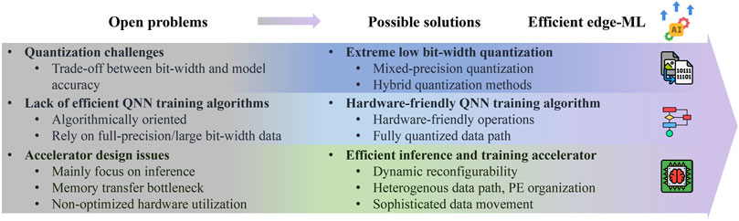
Figure 11. Technology advancements towards efficient edge machine learning (algorithm, hardware co-design).

6.1 Extreme low bit-width quantization

Figure 12 shows the influence of quantization precision on power consumption and latency with different hardware platforms. For MCU-based platforms, the latency and power consumption scale down with the quantization precision due to the fixed length of the arithmetic units. While for ASIC-based accelerators, the latency and power consumption scale down drastically with the quantization precision. With a simple dataset (CIFAR-10), the model accuracy experiences less degradation than a complex dataset (ImageNet) as the quantization precision decreases. Figure 12 shows that a close-to-FP accuracy can be obtained as the quantization bit-width is larger than 4-bit. Consequently, the majority of the QNN hardware designs shown in Table 3 adopt a quantization precision higher than 4-bit. Hence, there is a demand to improve model accuracy under sub-4-bit quantization scenarios. With low-bit quantization, the hardware platforms can be more energy efficient and fast, especially with ASIC-based platforms.

Figure 12

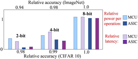
Figure 12. Qualitative study on relative power consumption per operation and latency under different precision quantization with MCU-oriented acceleration kernel (Garofalo et al., 2021) and ASIC-based NN accelerator (Ryu et al., 2022). Accuracy relative to full precision models is shown with the corresponding bit-width tested with CIFAR-10 (Yang et al., 2020) and ImageNet dataset (Zhang et al., 2018).

6.2 Study of the quantization of biases and batch normalization parameters during training

Compared to training, biases and batch normalization parameters can be fused into the following layer during inference. There are no studies offering a systematic discussion or implementation of quantization towards biases or batch normalization parameters during training. Meanwhile, comparing the accuracy resulting from cases with and without biases or affine operations (Figure 7), these operations play an important role in guaranteeing high performance accuracy. Hence, there is a strong demand for a systematic study of the quantization algorithms towards biases and batch normalization parameters during training. Only with quantized biases and batch normalization parameters expensive floating-point operations can be completely removed from the data path, which is a key point for efficient hardware accelerator design that supports training.

6.3 QNN training methods relying only on hardware-friendly operations (integer arithmetic operation, shift, bit-wise operation)

All QNN training methods depend on floating-point or long bit-width fixed-point parameters to accumulate the gradient preventing them from being deployed on low-end edge or IoT devices. At the same time, out of privacy concerns, machine learning methods, e.g., federated learning, require local training on low-end devices. Since there are some existing works (Sun et al., 2018b; Zhou et al., 2016; Sun et al., 2020) supporting the quantization of gradients during the backpropagation, the critical part of developing QNN training methods relying only on hardware-friendly operations is finding a substitution of the floating-point format in accumulating gradients. Therefore, it is worth exploring the fusion of new gradient accumulating methods and existing gradient quantization methods.

6.4 Hardware accelerator design supporting both efficient inference and training

The existing hardware accelerator designs focus more on inference rather than training assuming that costly training can be performed on powerful servers or clusters. However, as IoT technology, edge computing, and corresponding privacy concerns arise, it is required to switch neural network training from a centralized manner to a more distributed one. This trend puts a requirement on the hardware design to support not only the inference but also training. As analyzed in the previous sections, different data in the neural network, like weights, activations, and gradients, possess different ranges and distributions. This results in different types of quantization methods being applied to different data. To support both inference and training, the hardware architecture should be based on a heterogeneous design and compatible with various quantization methods and support arithmetic operations and corresponding data formats while maintaining high efficiency.

6.5 Dynamically reconfigurable accelerator designs

In addition to inference and training support, hardware reconfigurability is also critical. The edge device (e.g., mobile phone) may be required to run different applications and tasks. Neural networks running on the hardware accelerator could have different network structures, quantization methods, precision, and execution time requirements. All these factors bring challenges to the hardware design to be dynamically reconfigurable, especially in ASIC and non-volatile memory-based hardware architectures.

7 Conclusion

In light of the swift advancement of edge computing, this paper undertakes a comprehensive, integrative survey on CNN architectures, quantization algorithms, and QCNN accelerators with a focus on energy-efficient on-edge applications. Various existing QNN accelerator designs based on ASIC, FPGA, and non-volatile memory together with commonly adopted CNN models and quantization algorithms are introduced and analyzed. On top of that, we highlight general guidelines regarding QNN software-hardware co-designs and give future research directions considering both algorithm and hardware perspectives. Concurrently, notable advancements in CNN architectures and quantization algorithms, which have yet to find common application in QCNN accelerators and thus fall outside the ambit of this review, have been made. It is anticipated that these developments will significantly influence the future evolution of QCNN accelerator designs.

Author contributions

LZ: Conceptualization, Data curation, Formal Analysis, Investigation, Methodology, Software, Validation, Visualization, Writing – original draft, Writing – review and editing. OK: Data curation, Formal Analysis, Investigation, Methodology, Software, Validation, Writing – original draft, Writing – review and editing. MF: Writing – review and editing. AE: Funding acquisition, Project administration, Resources, Supervision, Writing – review and editing. KS: Funding acquisition, Project administration, Resources, Supervision, Writing – review and editing.

Funding

The author(s) declare that financial support was received for the research and/or publication of this article. This work is supported by the King Abdullah University of Science and Technology (KAUST) through the Competitive Research Grant program under grant URF/1/4704-01-01.

Acknowledgments

ChatGPT 4o, o4-mini-high models by OpenAI are used for grammar checking and text elaboration.

Conflict of interest

Author MF was employed by San Francisco Inc. CA.

The remaining authors declare that the research was conducted in the absence of any commercial or financial relationships that could be construed as a potential conflict of interest.

The author(s) declared that they were an editorial board member of Frontiers, at the time of submission. This had no impact on the peer review process and the final decision.

Publisher’s note

All claims expressed in this article are solely those of the authors and do not necessarily represent those of their affiliated organizations, or those of the publisher, the editors and the reviewers. Any product that may be evaluated in this article, or claim that may be made by its manufacturer, is not guaranteed or endorsed by the publisher.

References

Ankit, A., Hajj, I. E., Chalamalasetti, S. R., Ndu, G., Foltin, M., Williams, R. S., et al. (2019). “PUMA: a programmable ultra-efficient memristor-based accelerator for machine learning inference,” in Proceedings of the twenty-fourth international conference on architectural support for programming languages and operating systems, 715–731.

Google Scholar

Bai, Y., Wang, Y.-X., and Liberty, E. (2018). ProxQuant: quantized neural networks via proximal operators. arXiv Prepr. arXiv:1810.00861.

Google Scholar

Banner, R., Hubara, I., Hoffer, E., and Soudry, D. (2018). Scalable methods for 8-bit training of neural networks. Adv. neural Inf. Process. Syst. 31.

Google Scholar

Bengio, Y. (2013). Estimating or propagating gradients through stochastic neurons.

Google Scholar

Benmeziane, H., Maghraoui, K. E., Ouarnoughi, H., Niar, S., Wistuba, M., and Wang, N. (2021). A comprehensive survey on hardware-aware neural architecture search. arXiv preprint arXiv:2101.09336

Google Scholar

Bernstein, J., Zhao, J., Meister, M., Liu, M.-Y., Anandkumar, A., and Yue, Y. (2020). Learning compositional functions via multiplicative weight updates. Adv. neural Inf. Process. Syst. 33, 13319–13330.

Google Scholar

Biswas, A., and Chandrakasan, A. P. (2018). CONV-SRAM: an energy-efficient SRAM with in-memory dot-product computation for low-power convolutional neural networks. IEEE J. Solid-State Circuits 54, 217–230. doi:10.1109/jssc.2018.2880918

CrossRef Full Text | Google Scholar

Chang, K.-W., and Chang, T.-S. (2019). VWA: hardware efficient vectorwise accelerator for convolutional neural network. IEEE Trans. Circuits Syst. I Regul. Pap. 67, 145–154. doi:10.1109/tcsi.2019.2942529

CrossRef Full Text | Google Scholar

Chang, S.-E., Li, Y., Sun, M., Shi, R., So, H. K.-H., Qian, X., et al. (2021). “Mix and match: a novel FPGA-centric deep neural network quantization framework,” in 2021 IEEE international Symposium on high-performance computer architecture (HPCA) (IEEE), 208–220.

Google Scholar

Chen, D., Guo, Z., Fang, J., Zhao, C., Jiang, J., Zhou, K., et al. (2022). A 1T2R1C ReRAM CIM accelerator with energy-efficient voltage division and capacitive coupling for CNN acceleration in AI edge applications. IEEE Trans. Circuits Syst. II Express Briefs 70, 276–280. doi:10.1109/tcsii.2022.3201367

CrossRef Full Text | Google Scholar

Chen, J., Liu, L., Liu, Y., and Zeng, X. (2020). A learning framework for n-bit quantized neural networks toward fpgas. IEEE Trans. Neural Netw. Learn. Syst. 32, 1067–1081. doi:10.1109/tnnls.2020.2980041

PubMed Abstract | CrossRef Full Text | Google Scholar

Chen, Y., Li, J., Xiao, H., Jin, X., Yan, S., and Feng, J. (2017). Dual path networks. Adv. Neural Inf. Process. Syst. 30.

Google Scholar

Chen, Y.-H., Krishna, T., Emer, J. S., and Sze, V. (2016). Eyeriss: an energy-efficient reconfigurable accelerator for deep convolutional neural networks. IEEE J. solid-state circuits 52, 127–138. doi:10.1109/jssc.2016.2616357

CrossRef Full Text | Google Scholar

Chen, Y.-H., Yang, T.-J., Emer, J., and Sze, V. (2019). Eyeriss V2: a flexible accelerator for emerging deep neural networks on mobile devices. IEEE J. Emerg. Sel. Top. Circuits Syst. 9, 292–308. doi:10.1109/jetcas.2019.2910232

CrossRef Full Text | Google Scholar

Choi, J., Wang, Z., Venkataramani, S., Chuang, P. I.-J., Srinivasan, V., and Gopalakrishnan, K. (2018). PACT: parameterized clipping activation for quantized neural networks.

Google Scholar

Chu, T., Luo, Q., Yang, J., and Huang, X. (2021). Mixed-precision quantized neural networks with progressively decreasing bitwidth. Pattern Recognit. 111, 107647. doi:10.1016/j.patcog.2020.107647

CrossRef Full Text | Google Scholar

Courbariaux, M., Bengio, Y., and David, J.-P. (2015). Binaryconnect: training deep neural networks with binary weights during propagations. Adv. neural Inf. Process. Syst. 28.

Google Scholar

Denton, E. L., Zaremba, W., Bruna, J., LeCun, Y., and Fergus, R. (2014). Exploiting linear structure within convolutional networks for efficient evaluation. Adv. neural Inf. Process. Syst. 27.

Google Scholar

Ding, R., Liu, Z., Blanton, R. S., and Marculescu, D. (2018). “Quantized deep neural networks for energy efficient hardware-based inference,” in 2018 23rd asia and south pacific design automation conference (ASP-DAC IEEE), 1–8.

CrossRef Full Text | Google Scholar

Ding, R., Liu, Z., Chin, T.-W., Marculescu, D., and Blanton, R. D. (2019). “FLightNNs: lightweight quantized deep neural networks for fast and accurate inference,” in Proceedings of the 56th annual design automation conference 2019, 1–6.

Google Scholar

Ding, R., Liu, Z., Shi, R., Marculescu, D., and Blanton, R. (2017). “LightNN: filling the gap between conventional deep neural networks and binarized networks,” in Proceedings of the on great lakes symposium on VLSI 2017, 35–40.

Google Scholar

Elthakeb, A., Pilligundla, P., Mireshghallah, F., Yazdanbakhsh, A., Gao, S., and Esmaeilzadeh, H. (2019). “ReLeQ: an automatic reinforcement learning approach for deep quantization of neural networks,” in NeurIPS ML for systems workshop.

Google Scholar

Fiesler, E., Choudry, A., and Caulfield, H. J. (1990). “Weight discretization paradigm for optical neural networks,” SPIE. Opt. interconnections Netw., 1281. 164–173. doi:10.1117/12.20700

CrossRef Full Text | Google Scholar

Fukushima, K. (1980). Neocognitron: a self-organizing neural network model for a mechanism of pattern recognition unaffected by shift in position. Biol. Cybern. 36, 193–202. doi:10.1007/BF00344251

PubMed Abstract | CrossRef Full Text | Google Scholar

Gao, S.-H., Cheng, M.-M., Zhao, K., Zhang, X.-Y., Yang, M.-H., and Torr, P. (2019). Res2net: a new multi-scale backbone architecture. IEEE Trans. pattern analysis Mach. Intell. 43, 652–662. doi:10.1109/tpami.2019.2938758

PubMed Abstract | CrossRef Full Text | Google Scholar

Garofalo, A., Tagliavini, G., Conti, F., Benini, L., and Rossi, D. (2021). XpulpNN: enabling energy efficient and flexible inference of quantized neural networks on RISC-V based IoT end nodes. IEEE Trans. Emerg. Top. Comput. 9, 1489–1505. doi:10.1109/tetc.2021.3072337

CrossRef Full Text | Google Scholar

Gholami, A., Kim, S., Dong, Z., Yao, Z., Mahoney, M. W., and Keutzer, K. (2021). A survey of quantization methods for efficient neural network inference.

Google Scholar

Gi, S.-G., Lee, H., Jang, J., and Lee, B.-G. (2022). A reram-based convolutional neural network accelerator using the analog layer normalization technique. IEEE Trans. Industrial Electron. 70, 6442–6451. doi:10.1109/tie.2022.3190876

CrossRef Full Text | Google Scholar

Gong, R., Liu, X., Jiang, S., Li, T., Hu, P., Lin, J., et al. (2019). “Differentiable soft quantization: bridging full-precision and low-bit neural networks,” in Proceedings of the IEEE/CVF international conference on computer vision, 4852–4861.

Google Scholar

Gong, Y., Liu, L., Yang, M., and Bourdev, L. D. (2014). Compressing deep convolutional networks using vector quantization. Corr. abs/1412, 6115.

Google Scholar

Guo, J., Han, K., Wu, H., Tang, Y., Chen, X., Wang, Y., et al. (2022). “Cmt: convolutional neural networks meet vision transformers,” in Proceedings of the IEEE/CVF conference on computer vision and pattern recognition, 12175–12185.

Google Scholar

Guo, P., Ma, H., Chen, R., Li, P., Xie, S., and Wang, D. (2018). “FBNA: a fully binarized neural network accelerator,” in 2018 28th international conference on field programmable logic and applications (FPL) IEEE, 51–513.

Google Scholar

Guo, W., Fouda, M. E., Yantir, H. E., Eltawil, A. M., and Salama, K. N. (2020). Unsupervised adaptive weight pruning for energy-efficient neuromorphic systems. Front. Neurosci. 14, 598876. doi:10.3389/fnins.2020.598876

PubMed Abstract | CrossRef Full Text | Google Scholar

Guo, Y. (2018). A survey on methods and theories of quantized neural networks.

Google Scholar

Gupta, S., Agrawal, A., Gopalakrishnan, K., and Narayanan, P. (2015). “Deep learning with limited numerical precision,” in International conference on machine learning (PMLR) (Association for Computing Machinery), 1737–1746.

Google Scholar

Habi, H. V., Jennings, R. H., and Netzer, A. (2020). “HMQ: hardware friendly mixed precision quantization block for cnns,” in European conference on computer vision (Springer), 448–463.

Google Scholar

Han, S., Mao, H., and Dally, W. J. (2015). Deep compression: compressing deep neural networks with pruning, trained quantization and huffman coding.

Google Scholar

Hanif, M. A., and Shafique, M. (2022). A cross-layer approach towards developing efficient embedded deep learning systems. Microprocess. Microsystems 88, 103609. doi:10.1016/j.micpro.2020.103609

CrossRef Full Text | Google Scholar

Hashemi, S., Anthony, N., Tann, H., Bahar, R. I., and Reda, S. (2017). “Understanding the impact of precision quantization on the accuracy and energy of neural networks,” in Design, automation and test in europe conference and exhibition (DATE) (IEEE), 1474–1479.

Google Scholar

He, K., Zhang, X., Ren, S., and Sun, J. (2016). “Deep residual learning for image recognition,” in Proceedings of the IEEE conference on computer vision and pattern recognition, 770–778.

Google Scholar

Heo, B., Lee, M., Yun, S., and Choi, J. Y. (2019). Knowledge transfer via distillation of activation boundaries formed by hidden neurons. Proc. AAAI Conf. Artif. Intell. 33, 3779–3787. doi:10.1609/aaai.v33i01.33013779

CrossRef Full Text | Google Scholar

Hinton, G., Vinyals, O., and Dean, J. (2015). Distilling the knowledge in a neural network.

Google Scholar

Howard, A. G., Zhu, M., Chen, B., Kalenichenko, D., Wang, W., Weyand, T., et al. (2017). MobileNets: efficient convolutional neural networks for mobile vision applications.

Google Scholar

Hu, X., Li, X., Huang, H., Zheng, X., and Xiong, X. (2022). TiNNA: a tiny accelerator for neural networks with efficient dsp optimization. IEEE Trans. Circuits Syst. II Express Briefs 69, 2301–2305. doi:10.1109/tcsii.2022.3150980

CrossRef Full Text | Google Scholar

Hubara, I., Courbariaux, M., Soudry, D., El-Yaniv, R., and Bengio, Y. (2017). Quantized neural networks: training neural networks with low precision weights and activations. J. Mach. Learn. Res. 18, 6869–6898.

Google Scholar

Ioffe, S., and Szegedy, C. (2015). “Batch normalization: accelerating deep network training by reducing internal covariate shift,” in International conference on machine learning (PMLR) (Association for Computing Machinery), 448–456.

Google Scholar

Jacob, B., Kligys, S., Chen, B., Zhu, M., Tang, M., Howard, A., et al. (2018). “Quantization and training of neural networks for efficient integer-arithmetic-only inference,” in Proceedings of the IEEE conference on computer vision and pattern recognition, 2704–2713.

Google Scholar

Jaderberg, M., Vedaldi, A., and Zisserman, A. (2014). Speeding up convolutional neural networks with low rank expansions, 88.1–88.13. doi:10.5244/c.28.88

CrossRef Full Text | Google Scholar

Janowsky, S. A. (1989). Pruning versus clipping in neural networks. Phys. Rev. A 39, 6600–6603. doi:10.1103/PhysRevA.39.6600

PubMed Abstract | CrossRef Full Text | Google Scholar

Jiang, H., Li, Q., and Li, Y. (2022). “Post training quantization after neural network,” in 2022 14th international conference on computer research and development (ICCRD) (IEEE), 1–6.

CrossRef Full Text | Google Scholar

Jiao, Y., Han, L., Jin, R., Su, Y.-J., Ho, C., Yin, L., et al. (2020). “7.2 a 12nm programmable convolution-efficient neural-processing-unit chip achieving 825tops,” in 2020 IEEE international solid-state circuits conference-(ISSCC) (IEEE), 136–140.

Google Scholar

Kim, H., Jung, Y., and Kim, L.-S. (2022). ADC-Free ReRAM-based in-situ accelerator for energy-efficient binary neural networks. IEEE Trans. Comput. 73, 353–365. doi:10.1109/tc.2022.3224800

CrossRef Full Text | Google Scholar

Kim, N., Shin, D., Choi, W., Kim, G., and Park, J. (2020). Exploiting retraining-based mixed-precision quantization for low-cost dnn accelerator design. IEEE Trans. Neural Netw. Learn. Syst. 32, 2925–2938. doi:10.1109/tnnls.2020.3008996

PubMed Abstract | CrossRef Full Text | Google Scholar

Krestinskaya, O., Fouda, M. E., Benmeziane, H., El Maghraoui, K., Sebastian, A., Lu, W. D., et al. (2024a). Neural architecture search for in-memory computing-based deep learning accelerators. Nat. Rev. Electr. Eng. 1, 374–390. doi:10.1038/s44287-024-00052-7

CrossRef Full Text | Google Scholar

Krestinskaya, O., Fouda, M. E., Eltawil, A., and Salama, K. N. (2024b). Towards efficient imc accelerator design through joint hardware-workload co-optimization.

Google Scholar

Krestinskaya, O., Irmanova, A., and James, A. P. (2019). “Memristive non-idealities: is there any practical implications for designing neural network chips?,” in 2019 IEEE international Symposium on Circuits and systems (ISCAS) (IEEE), 1–5.

Google Scholar

Krestinskaya, O., and James, A. P. (2020). Analogue neuro-memristive convolutional dropout nets. Proc. R. Soc. A 476, 20200210. doi:10.1098/rspa.2020.0210

CrossRef Full Text | Google Scholar

Krestinskaya, O., Salama, K. N., and James, A. P. (2018). “Analog backpropagation learning circuits for memristive crossbar neural networks,” in 2018 IEEE international symposium on circuits and systems (ISCAS), 1–5. doi:10.1109/ISCAS.2018.8351344

CrossRef Full Text | Google Scholar

Krestinskaya, O., Zhang, L., and Salama, K. N. (2022). “Towards efficient rram-based quantized neural networks hardware: state-of-the-art and open issues,” in 2022 IEEE 22nd international conference on nanotechnology (NANO) (IEEE), 465–468.

CrossRef Full Text | Google Scholar

Krestinskaya, O., Zhang, L., and Salama, K. N. (2023). Towards efficient in-memory computing hardware for quantized neural networks: state-of-the-art, open challenges and perspectives. IEEE Trans. Nanotechnol. 22, 377–386. doi:10.1109/TNANO.2023.3293026

CrossRef Full Text | Google Scholar

Krishnamoorthi, R. (2018). Quantizing deep convolutional networks for efficient inference: a whitepaper.

Google Scholar

Krizhevsky, A., Sutskever, I., and Hinton, G. E. (2017). Imagenet classification with deep convolutional neural networks. Commun. ACM 60, 84–90. doi:10.1145/3065386

CrossRef Full Text | Google Scholar

Kulkarni, U., Hosamani, A. S., Masur, A. S., Hegde, S., Vernekar, G. R., and Chandana, K. S. (2022). “A survey on quantization methods for optimization of deep neural networks,” in 2022 international conference on automation, computing and renewable systems (ICACRS) (IEEE), 827–834.

CrossRef Full Text | Google Scholar

LeCun, Y., Boser, B., Denker, J. S., Henderson, D., Howard, R. E., Hubbard, W., et al. (1989). Backpropagation applied to handwritten zip code recognition. Neural Comput. 1, 541–551. doi:10.1162/neco.1989.1.4.541

CrossRef Full Text | Google Scholar

Lecun, Y., Bottou, L., Bengio, Y., and Haffner, P. (1998). Gradient-based learning applied to document recognition. Proc. IEEE 86, 2278–2324. doi:10.1109/5.726791

CrossRef Full Text | Google Scholar

Lee, C.-Y., Gallagher, P. W., and Tu, Z. (2016). “Generalizing pooling functions in convolutional neural networks: mixed, gated, and tree,” in Artificial intelligence and statistics (PMLR), 464–472.

Google Scholar

Lee, J., Kim, C., Kang, S., Shin, D., Kim, S., and Yoo, H.-J. (2018). UNPU: an energy-efficient deep neural network accelerator with fully variable weight bit precision. IEEE J. Solid-State Circuits 54, 173–185. doi:10.1109/jssc.2018.2865489

CrossRef Full Text | Google Scholar

Lee, J., Shin, D., and Yoo, H.-J. (2017). “A 21mw low-power recurrent neural network accelerator with quantization tables for embedded deep learning applications,” in 2017 IEEE asian solid-state circuits conference (A-SSCC) (IEEE), 237–240.

Google Scholar

Lee, S. K., Agrawal, A., Silberman, J., Ziegler, M., Kang, M., Venkataramani, S., et al. (2021a). A 7-nm four-core mixed-precision ai chip with 26.2-tflops hybrid-fp8 training, 104.9-tops int4 inference, and workload-aware throttling. IEEE J. Solid-State Circuits 57, 182–197. doi:10.1109/jssc.2021.3120113

CrossRef Full Text | Google Scholar

Lee, Y. S., Chung, E.-Y., Gong, Y.-H., and Chung, S. W. (2021b). Quant-PIM: an energy-efficient processing-in-memory accelerator for layerwise quantized neural networks. IEEE Embed. Syst. Lett. 13, 162–165. doi:10.1109/les.2021.3050253

CrossRef Full Text | Google Scholar

Leroux, S., Vankeirsbilck, B., Verbelen, T., Simoens, P., and Dhoedt, B. (2020). Training binary neural networks with knowledge transfer. Neurocomputing 396, 534–541. doi:10.1016/j.neucom.2018.09.103

CrossRef Full Text | Google Scholar

Li, Y., Shen, M., Ma, J., Ren, Y., Zhao, M., Zhang, Q., et al. (2021). MQBench: towards reproducible and deployable model quantization benchmark.

Google Scholar

Li, Y., Wang, W., Bai, H., Gong, R., Dong, X., and Yu, F. (2020). Efficient bitwidth search for practical mixed precision neural network.

Google Scholar

Lin, C.-H., Cheng, C.-C., Tsai, Y.-M., Hung, S.-J., Kuo, Y.-T., Wang, P. H., et al. (2020a). “7.1 a 3.4-to-13.3 tops/w 3.6 tops dual-core deep-learning accelerator for versatile ai applications in 7nm 5g smartphone soc,” in 2020 ieee international solid-state circuits conference-(isscc) (IEEE), 134–136.

Google Scholar

Lin, J., Chen, W.-M., Cai, H., Gan, C., and Han, S. (2021). MCUNetV2: memory-efficient patch-based inference for tiny deep learning. arXiv preprint arXiv:2110.15352

Google Scholar

Lin, J., Chen, W.-M., Lin, Y., Gan, C., and Han, S. (2020b). MCUNet: tiny deep learning on iot devices. Adv. Neural Inf. Process. Syst. 33, 11711–11722.

Google Scholar

Liu, C.-N., Lai, Y.-A., Kuo, C.-H., and Zhan, S.-A. (2021). “Design of 2d systolic array accelerator for quantized convolutional neural networks,” in 2021 international symposium on VLSI design, automation and test (VLSI-DAT) (IEEE), 1–4.

CrossRef Full Text | Google Scholar

Liu, Z., Wu, B., Luo, W., Yang, X., Liu, W., and Cheng, K.-T. (2018). “Bi-Real Net: enhancing the performance of 1-bit cnns with improved representational capability and advanced training algorithm,” in Proceedings of the European conference on computer vision (ECCV) (Springer), 722–737.

Google Scholar

Ma, Y., Jin, T., Zheng, X., Wang, Y., Li, H., Jiang, G., et al. (2021). OMPQ: orthogonal mixed precision quantization.

Google Scholar

Martinez, B., Yang, J., Bulat, A., and Tzimiropoulos, G. (2020). Training binary neural networks with real-to-binary convolutions

Google Scholar

Matinizadeh, S., Mohammadhassani, A., Pacik-Nelson, N., Polykretisl, I., Mishra, A., Shackleford, J., et al. (2024). “A fully-configurable digital spiking neuromorphic hardware design with variable quantization and mixed precision,” in 2024 IEEE 67th international midwest symposium on circuits and systems (MWSCAS) (IEEE), 937–941.

CrossRef Full Text | Google Scholar

Menghani, G. (2023). Efficient deep learning: a survey on making deep learning models smaller, faster, and better. ACM Comput. Surv. 55, 1–37. doi:10.1145/3578938

CrossRef Full Text | Google Scholar

Moon, S., Lee, K.-J., Mun, H.-G., Kim, B., and Sim, J.-Y. (2022). An 8.9–71.3 tops/w deep learning accelerator for arbitrarily quantized neural networks. IEEE Trans. Circuits Syst. II Express Briefs 69, 4148–4152. doi:10.1109/tcsii.2022.3185184

CrossRef Full Text | Google Scholar

Moons, B., Uytterhoeven, R., Dehaene, W., and Verhelst, M. (2017). “14.5 envision: a 0.26-to-10tops/w subword-parallel dynamic-voltage-accuracy-frequency-scalable convolutional neural network processor in 28nm fdsoi,” in 2017 IEEE international solid-state circuits conference (ISSCC) (IEEE), 246–247.

Google Scholar

Mrazek, V., Vasícek, Z., Sekanina, L., Hanif, M. A., and Shafique, M. (2019). “ALWANN: automatic layer-wise approximation of deep neural network accelerators without retraining,” in 2019 IEEE/ACM international conference on computer-aided design (ICCAD) (IEEE), 1–8.

CrossRef Full Text | Google Scholar

Neill, J. O. (2020). An overview of neural network compression

Google Scholar

Netzer, Y., Wang, T., Coates, A., Bissacco, A., Wu, B., and Ng, A. Y. (2011). Reading digits in natural images with unsupervised feature learning

Google Scholar

Nguyen, D. T., Kim, H., and Lee, H.-J. (2020). Layer-specific optimization for mixed data flow with mixed precision in fpga design for cnn-based object detectors. IEEE Trans. Circuits Syst. Video Technol. 31, 2450–2464. doi:10.1109/tcsvt.2020.3020569

CrossRef Full Text | Google Scholar

Nvidia (2024). TensorRT homepage. Available online at: https://developer.nvidia.com/tensorrt.

Google Scholar

ONNX (2024). ONNX homepage. Available online at: https://onnx.ai/index.html.

Google Scholar

Park, E., Ahn, J., and Yoo, S. (2017). “Weighted-entropy-based quantization for deep neural networks,” in Proceedings of the IEEE conference on computer vision and pattern recognition, 5456–5464.

Google Scholar

Pham, H., Dai, Z., Xie, Q., and Le, Q. V. (2021). “Meta pseudo labels,” in Proceedings of the IEEE/CVF conference on computer vision and pattern recognition, 11557–11568.

Google Scholar

Qin, H., Gong, R., Liu, X., Bai, X., Song, J., and Sebe, N. (2020). Binary neural networks: a survey. Pattern Recognit. 105, 107281. doi:10.1016/j.patcog.2020.107281

CrossRef Full Text | Google Scholar

Qiu, J., Wang, J., Yao, S., Guo, K., Li, B., Zhou, E., et al. (2016). “Going deeper with embedded fpga platform for convolutional neural network,” in Proceedings of the 2016 ACM/SIGDA international symposium on field-programmable gate arrays, 26–35.

Google Scholar

Rakka, M., Fouda, M. E., Khargonekar, P., and Kurdahi, F. (2022). Mixed-precision neural networks: a survey

Google Scholar

Rastegari, M., Ordonez, V., Redmon, J., and Farhadi, A. (2016). “XNOR-Net: imagenet classification using binary convolutional neural networks,” in European conference on computer vision (Springer), 525–542.

Google Scholar

Rokh, B., Azarpeyvand, A., and Khanteymoori, A. (2022). A comprehensive survey on model quantization for deep neural networks

Google Scholar

Rotem, N., Fix, J., Abdulrasool, S., Catron, G., Deng, S., Dzhabarov, R., et al. (2018). Glow: graph lowering compiler techniques for neural networks.

Google Scholar

Ryu, S., Kim, H., Yi, W., Kim, E., Kim, Y., Kim, T., et al. (2022). Bitblade: energy-efficient variable bit-precision hardware accelerator for quantized neural networks. IEEE J. Solid-State Circuits 57, 1924–1935. doi:10.1109/jssc.2022.3141050

CrossRef Full Text | Google Scholar

Ryu, S., Kim, H., Yi, W., and Kim, J.-J. (2019). “Bitblade: area and energy-efficient precision-scalable neural network accelerator with bitwise summation,” in Proceedings of the 56th annual design automation conference 2019, 1–6.

Google Scholar

Ryu, S., Kim, H., Yi, W., Koo, J., Kim, E., Kim, Y., et al. (2020). “A 44.1 tops/w precision-scalable accelerator for quantized neural networks in 28nm cmos,” in 2020 IEEE custom integrated circuits conference (CICC) (IEEE), 1–4.

CrossRef Full Text | Google Scholar

Sakr, C., Dai, S., Venkatesan, R., Zimmer, B., Dally, W., and Khailany, B. (2022). “Optimal clipping and magnitude-aware differentiation for improved quantization-aware training,” in International conference on machine learning (PMLR), (Association for Computing Machinery), 19123–19138.

Google Scholar

Sandler, M., Howard, A., Zhu, M., Zhmoginov, A., and Chen, L.-C. (2018). “MobileNetV2: inverted residuals and linear bottlenecks,” in Proceedings of the IEEE conference on computer vision and pattern recognition, 4510–4520.

Google Scholar

Shafiee, A., Nag, A., Muralimanohar, N., Balasubramonian, R., Strachan, J. P., Hu, M., et al. (2016). ISAAC: a convolutional neural network accelerator with in-situ analog arithmetic in crossbars. ACM SIGARCH Comput. Archit. News 44, 14–26. doi:10.1145/3007787.3001139

CrossRef Full Text | Google Scholar

Sharma, H., Park, J., Suda, N., Lai, L., Chau, B., Chandra, V., et al. (2018). “Bit Fusion: bit-level dynamically composable architecture for accelerating deep neural network,” in 2018 ACM/IEEE 45th annual international symposium on computer architecture (ISCA) (IEEE), 764–775.

Google Scholar

Shen, A., Lai, Z., and Li, D. (2024a). “Exploring quantization techniques for large-scale language models: methods, challenges and future directions,” in Proceedings of the 2024 9th international conference on cyber security and information engineering, 783–790.

Google Scholar

Shen, G., Zhao, D., Li, T., Li, J., and Zeng, Y. (2024b). “Are conventional snns really efficient? a perspective from network quantization,” in Proceedings of the IEEE/CVF conference on computer vision and pattern recognition, 27538–27547.

Google Scholar

Shin, D., Lee, J., Lee, J., and Yoo, H.-J. (2017). “14.2 DNPU: an 8.1 tops/w reconfigurable cnn-rnn processor for general-purpose deep neural networks,” in 2017 IEEE international solid-state circuits conference (ISSCC) (IEEE), 240–241.

Google Scholar

Siddegowda, S., Fournarakis, M., Nagel, M., Blankevoort, T., Patel, C., and Khobare, A. (2022). Neural network quantization with ai model efficiency toolkit aimet

Google Scholar

Sifre, L., and Mallat, S. (2014). Rigid-motion scattering for texture classification.

Google Scholar

Simonyan, K., and Zisserman, A. (2014). Very deep convolutional networks for large-scale image recognition.

Google Scholar

Smagulova, K., Fouda, M. E., Kurdahi, F., Salama, K. N., and Eltawil, A. (2023). Resistive neural hardware accelerators. Proc. IEEE 111, 500–527. doi:10.1109/jproc.2023.3268092

CrossRef Full Text | Google Scholar

Song, L., Qian, X., Li, H., and Chen, Y. (2017). “PipeLayer: a pipelined ReRAM-based accelerator for deep learning,” in 2017 IEEE international symposium on high performance computer architecture (HPCA) (IEEE), 541–552.

CrossRef Full Text | Google Scholar

Spallanzani, M., Cavigelli, L., Leonardi, G. P., Bertogna, M., and Benini, L. (2019). Additive noise annealing and approximation properties of quantized neural networks

Google Scholar

Srivastava, N., Hinton, G., Krizhevsky, A., Sutskever, I., and Salakhutdinov, R. (2014). Dropout: a simple way to prevent neural networks from overfitting. J. Mach. Learn. Res. 15, 1929–1958.

Google Scholar

Sun, M., Li, Z., Lu, A., Li, Y., Chang, S.-E., Ma, X., et al. (2022). FILM-QNN: efficient FPGA acceleration of deep neural networks with intra-layer, mixed-precision quantization, 134, 145. doi:10.1145/3490422.3502364

CrossRef Full Text | Google Scholar

Sun, X., Peng, X., Chen, P.-Y., Liu, R., Seo, J.-s., and Yu, S. (2018a). “Fully parallel rram synaptic array for implementing binary neural network with (+1,- 1) weights and (+1, 0) neurons,” in 2018 23rd asia and south pacific design automation conference (ASP-DAC IEEE), 574–579.

CrossRef Full Text | Google Scholar

Sun, X., Wang, N., Chen, C.-Y., Ni, J., Agrawal, A., Cui, X., et al. (2020). Ultra-low precision 4-bit training of deep neural networks. Adv. Neural Inf. Process. Syst. 33, 1796–1807.

Google Scholar

Sun, X., Yin, S., Peng, X., Liu, R., Seo, J.-s., and Yu, S. (2018b). “XNOR-RRAM: a scalable and parallel resistive synaptic architecture for binary neural networks,” in 2018 design, automation and test in europe conference and exhibition (DATE) (IEEE), 1423–1428.

Google Scholar

Tan, M., and Le, Q. (2019). “EfficientNet: rethinking model scaling for convolutional neural networks,” in International conference on machine learning (PMLR), (Association for Computing Machinery), 6105–6114.

Google Scholar

Tang, W., Hua, G., and Wang, L. (2017). “How to train a compact binary neural network with high accuracy?,” in Thirty-First AAAI conference on artificial intelligence.

Google Scholar

Teng, C.-F., Wu, C.-H. D., Ho, A. K.-S., and Wu, A.-Y. A. (2019). “Low-complexity recurrent neural network-based polar decoder with weight quantization mechanism,” in ICASSP 2019-2019 IEEE international conference on acoustics, speech and signal processing (ICASSP) (IEEE), 1413–1417.

Google Scholar

Ueyoshi, K., Ando, K., Hirose, K., Takamaeda-Yamazaki, S., Kadomoto, J., Miyata, T., et al. (2018). “QUEST: a 7.49 tops multi-purpose log-quantized dnn inference engine stacked on 96mb 3d sram using inductive-coupling technology in 40nm cmos,” in 2018 IEEE international solid-state circuits conference-(ISSCC) (IEEE), 216–218.

Google Scholar

Umuroglu, Y., Akhauri, Y., Fraser, N. J., and Blott, M. (2020). “LogicNets: Co-designed neural networks and circuits for extreme-throughput applications,” in 2020 30th international conference on field-programmable logic and applications (FPL) (IEEE), 291–297.

CrossRef Full Text | Google Scholar

Umuroglu, Y., Fraser, N. J., Gambardella, G., Blott, M., Leong, P., Jahre, M., et al. (2017). “FINN: a framework for fast, scalable binarized neural network inference,” in Proceedings of the 2017 ACM/SIGDA international symposium on field-programmable gate arrays, 65–74.

Google Scholar

Venkataramani, S., Ranjan, A., Roy, K., and Raghunathan, A. (2014). “Axnn: energy-efficient neuromorphic systems using approximate computing,” in Proceedings of the 2014 international symposium on Low power electronics and design, 27–32.

Google Scholar

Wang, J., Wang, X., Eckert, C., Subramaniyan, A., Das, R., Blaauw, D., et al. (2019a). A 28-nm compute sram with bit-serial logic/arithmetic operations for programmable in-memory vector computing. IEEE J. Solid-State Circuits 55, 76–86. doi:10.1109/jssc.2019.2939682

CrossRef Full Text | Google Scholar

Wang, K., Liu, Z., Lin, Y., Lin, J., and Han, S. (2020). Hardware-centric automl for mixed-precision quantization. Int. J. Comput. Vis. 128, 2035–2048. doi:10.1007/s11263-020-01339-6

CrossRef Full Text | Google Scholar

Wang, N., Choi, J., Brand, D., Chen, C.-Y., and Gopalakrishnan, K. (2018). Training deep neural networks with 8-bit floating point numbers. Adv. neural Inf. Process. Syst. 31.

Google Scholar

Wang, Q., Wang, X., Lee, S. H., Meng, F.-H., and Lu, W. D. (2019b). “A deep neural network accelerator based on tiled rram architecture,” in 2019 IEEE international electron devices meeting (IEDM) (IEEE), 14–4.

Google Scholar

Warden, P., and Situnayake, D. (2019). TinyML. O’Reilly Media, Inc.

Google Scholar

Wei, X., Liu, W., Chen, L., Ma, L., Chen, H., and Zhuang, Y. (2019). FPGA-based hybrid-type implementation of quantized neural networks for remote sensing applications. Sensors 19, 924. doi:10.3390/s19040924

PubMed Abstract | CrossRef Full Text | Google Scholar

Wu, C., Zhuang, J., Wang, K., and He, L. (2021). “MP-OPU: a mixed precision FPGA-based overlay processor for convolutional neural networks,” in 2021 31st international conference on field-programmable logic and applications (FPL) (IEEE), 33–37.

Google Scholar

Xiao, T. P., Feinberg, B., Bennett, C. H., Prabhakar, V., Saxena, P., Agrawal, V., et al. (2022). On the accuracy of analog neural network inference accelerators. IEEE Circuits Syst. Mag. 22, 26–48. doi:10.1109/mcas.2022.3214409

CrossRef Full Text | Google Scholar

Xu, J., Pan, Y., Pan, X., Hoi, S., Yi, Z., and Xu, Z. (2022). Regnet: self-regulated network for image classification. IEEE Trans. Neural Netw. Learn. Syst. 34, 9562–9567. doi:10.1109/tnnls.2022.3158966

PubMed Abstract | CrossRef Full Text | Google Scholar

Yang, J., Shen, X., Xing, J., Tian, X., Li, H., Deng, B., et al. (2019). “Quantization networks,” in Proceedings of the IEEE/CVF conference on computer vision and pattern recognition, 7308–7316.

Google Scholar

Yang, Z., Wang, Y., Han, K., Xu, C., Xu, C., Tao, D., et al. (2020). Searching for low-bit weights in quantized neural networks. Adv. neural Inf. Process. Syst. 33, 4091–4102.

Google Scholar

Yao, P., Wu, H., Gao, B., Tang, J., Zhang, Q., Zhang, W., et al. (2020). Fully hardware-implemented memristor convolutional neural network. Nature 577, 641–646. doi:10.1038/s41586-020-1942-4

PubMed Abstract | CrossRef Full Text | Google Scholar

Yao, Z., Dong, Z., Zheng, Z., Gholami, A., Yu, J., Tan, E., et al. (2021). “HAWQ-V3: dyadic neural network quantization,” in International conference on machine learning (PMLR), (Association for Computing Machinery), 11875–11886.

Google Scholar

Yin, S., Jiang, Z., Seo, J.-S., and Seok, M. (2020). XNOR-SRAM: in-memory computing sram macro for binary/ternary deep neural networks. IEEE J. Solid-State Circuits 55, 1–11. doi:10.1109/jssc.2019.2963616

CrossRef Full Text | Google Scholar

Zhang, D., Yang, J., Ye, D., and Hua, G. (2018). “LQ-Nets: learned quantization for highly accurate and compact deep neural networks,” in Proceedings of the European conference on computer vision (ECCV), 365–382.

Google Scholar

Zhang, Y., Pan, J., Liu, X., Chen, H., Chen, D., and Zhang, Z. (2021). “FracBNN: accurate and FPGA-efficient binary neural networks with fractional activations,” in The 2021 ACM/SIGDA international symposium on field-programmable gate arrays, 171–182.

Google Scholar

Zhao, J., Dai, S., Venkatesan, R., Zimmer, B., Ali, M., Liu, M.-Y., et al. (2022). LNS-Madam: low-precision training in logarithmic number system using multiplicative weight update. IEEE Trans. Comput. 71, 3179–3190. doi:10.1109/tc.2022.3202747

CrossRef Full Text | Google Scholar

Zhijie, Y., Lei, W., Li, L., Shiming, L., Shasha, G., and Shuquan, W. (2020). Bactran: a hardware batch normalization implementation for cnn training engine. IEEE Embed. Syst. Lett. 13, 29–32. doi:10.1109/les.2020.2975055

CrossRef Full Text | Google Scholar

Zhou, S., Wu, Y., Ni, Z., Zhou, X., Wen, H., and Zou, Y. (2016). DoReFa-Net: training low bitwidth convolutional neural networks with low bitwidth gradients

Google Scholar

Zhu, Z., Sun, H., Lin, Y., Dai, G., Xia, L., Han, S., et al. (2019). “A configurable multi-precision cnn computing framework based on single bit rram,” in 2019 56th ACM/IEEE design automation conference (DAC) (IEEE), 1–6.

Google Scholar

Zhuang, B., Shen, C., Tan, M., Liu, L., and Reid, I. (2018). “Towards effective low-bitwidth convolutional neural networks,” in Proceedings of the IEEE conference on computer vision and pattern recognition, 7920–7928.

Google Scholar