Dark Reduction Drives Evasion of Mercury From the Ocean

Introduction

Mercury (Hg) is a toxic trace metal that is uniquely volatile. Current estimates place the rate of gross evasion of mercury (Hg) from the ocean to the atmosphere at about 17 Mmole y⁻¹, which is close to the sum of inputs to the ocean of 21 Mmole y⁻¹ (e.g., Outridge et al., 2018). While these fluxes are nearly balanced in mass, they are very different in chemistry, with most of the input to the ocean from the atmosphere as Hg(II) and the Hg leaving the ocean to the air is mostly as Hg⁰. Thus, a substantial amount of Hg(II) reduction must take place in the ocean to support the observed fluxes. We can put the sea-air flux in context by noting that the Outridge et al. estimate for the amount of Hg in the surface water is about 13 Mmole. This value, when combined with the flux information, suggests a residence time of Hg in the surface ocean with respect to evasion of about 0.76 years and an apparent specific net reduction rate of 0.36 % day⁻¹. This apparent specific reduction rate is slower than that measured for gross production of Hg⁰ from Hg(II) (e.g., Rolfhus, 1998; Costa and Liss, 1999; Whalin et al., 2007; Fantozzi et al., 2009; Qureshi et al., 2010; Soerensen et al., 2014; Kuss et al., 2015; Lee and Fisher, 2019). If gross reduction proceeds faster than the loss of Hg⁰ from the surface ocean, then there must be substantial re-oxidation of Hg⁰ prior to evasion (e.g., Soerensen et al., 2010). This sets up the possibility that the concentration of Hg⁰ in the surface, one of the primary driving parameters for Hg evasion, is at or close to a steady-state set mostly by the redox recycling of Hg, and not the rate of evasion or net production.

To gain a greater understanding of the evasion of Hg from the ocean, much research has been conducted to understand the ways by which Hg(II) is reduced to Hg⁰ in seawater. Light-dependent mechanisms are fast (specific reduction with respect to gross photoreduction under ambient light conditions: 0.39 to 1.53 h⁻¹) and reduction mechanisms that appear not to be light-dependent have been found to be many times slower (specific reduction: <0.1 to 0.23 h⁻¹; Rolfhus, 1998; Costa and Liss, 1999; Whalin et al., 2007; Fantozzi et al., 2009; Qureshi et al., 2010). However, when integrated over a water column, as done by Rolfhus and Fitzgerald (2004) and alluded to by Fantozzi et al. (2009) and Kuss et al. (2015), the importance of dark reduction mechanisms increases, perhaps even to dominance because the light-dependent reactions slow down as light diminishes.

One recent study in seawater deserves special attention, that of Kuss et al. (2015) in the Baltic Sea. Using shipboard incubations and a variety of amendments (e.g., filter-sterilizing, light-shading), they sought to apportion the Hg⁰ produced within Baltic surface water between light and dark mechanisms. Their results suggested that about 59% was produced from light reactions (a combination of direct abiotic and indirect biotic) and about 41% from dark reactions (with some evidence that this process was at least partially biological). Kuss et al. noted, as did Rolfhus and Fitzgerald, that integrating to depths below the surface would likely boost the importance of dark reactions but did not calculate this.

The mechanism or mechanisms of Hg²⁺ reduction to Hg⁰ in the dark are unclear. In the light, charge-transfer reactions seem to be most important as photoreduction of Hg²⁺ is most effective when Hg is complexed with photoactive dissolved organic matter (O'Driscoll et al., 2006). However, photoreduction can be enhanced through the production of reactive transients such as Fe(II) which in turn reduce Hg²⁺ (Zhang and Lindberg, 2001). Thus, it is reasonable that any redox intermediates of sufficient strength produced by non-photochemical means should also be able to reduce Hg²⁺. Candidate species in the dark ocean most prominently include the reactive oxygen species (ROS) superoxide and hydrogen peroxide which have been shown to be actively produced by common marine heterotrophs (Diaz et al., 2013; Sutherland et al., 2019).

How relevant are the implications of these studies to the global ocean? The Baltic Sea is a low salinity and relatively eutrophicated marine environment, and the Long Island Sound where Rolfhus and Fitzgerald (2004) conducted their studies is an impacted marginal embayment and most of Whalin et al. (2007) work was conducted in estuarine environments. Thus, it remains uncertain as to how important dark reduction is in the open ocean. Here we describe experiments designed to provide additional constraint on the rates and possible mechanism(s) of dark reduction under such conditions and then place those rates in a global context through relatively simple modeling.

Methods

Sample Collection

Samples for profiles, diel studies and production incubations were collected during the TORCH 2 cruise from September 20th to 29th, 2017 on board the R/V Endeavor (EN604; C. Hansel, Chief Scientist). Trace metal-clean water collection was accomplished using cleaned 8-L X-Niskin bottles deployed from a 12-place Seabird Electronics rosette (SBE 19plus/SBE 32, the trace-metal rosette or TMR). The rosette also carried a CTD-driven Auto-firing Module (AFM). The AFM was programmed to close Niskin bottles during up-casts at depths selected by examining water column profiles of temperature, salinity, photosynthetically active radiation (PAR) and chlorophyll fluorescence that were collected with the ship's non-clean CTD system immediately before the TMR was deployed. Samples for vertical profiles were retrieved at 4–6 depths (with Niskins doubled- or tripled-up to provide the necessary volume for various needs) that also included depths that would represent those for further incubation studies.

The stations occupied during TORCH 2 cruise are summarized in Table 1 and shown in Figure 1. All except Station 4 can be characterized as continental shelf environments, while Station 4 is an off-shelf, more open ocean environment. The stations were selected to target a range of heterotrophic microbe activity, as reflected by a range of water temperature and primary production (Figures S1, S2).

TABLE 1

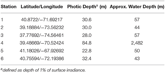
Table 1. Stations occupied during the TORCH 2 Cruise.

FIGURE 1

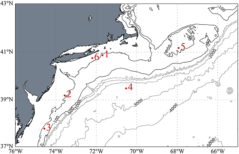
Figure 1. Station locations for the TORCH 2 cruise. Isobaths on the continental shelf are shown in solid lines and are in 50-meter intervals. Those off the shelf are shown in dotted lines and denote 1,000-meter intervals. Bathymetric data from ETOPO1.

Mercury Speciation

We measured the amount of dissolved total Hg and Hg⁰ according to protocols described elsewhere (Lamborg et al., 2012 and references therein). In brief, duplicate ~200 mL samples for dissolved total Hg were withdrawn from X-Niskins by peristaltic pump in a “clean bubble” by passing the fluid through Sterivex filter capsules with a nominal pore size of 0.2 μm and into 250-mL, acid-washed glass bottles (I-Chem). Similarly, but without filtration, duplicate ~1,800 mL samples for Hg⁰ were withdrawn from the X-Niskins by gravity through a length of acid-washed C-Flex tubing positioned to avoid injecting bubbles. Samples for total Hg were then preserved with BrCl, while the samples for Hg⁰ were immediately purged with high-purity N₂, with the gas effluent passing through a gold-coated sand trap to amalgamate Hg⁰. Following purging, the volume of the sample purged was measured by graduated cylinder to the nearest 5 mL. The amount of Hg⁰ so collected was determined by heating the trapping column onto the analytical trap of a Tekran 2600 Cold-vapor Atomic Fluorescence Spectrometer (CVAFS), calibrated using a saturated vapor standard held at 15 °C (Tekran). Total Hg samples were also measured by purge-and-trap CVAFS after the excess BrCl was reduced by NH₂OH and the Hg(II) present reduced to Hg⁰ by SnCl₂. Calibration was also accomplished using the vapor standard and checked with aqueous standards traceable to NIST.

Gross Hg⁰ Production Incubations

The aphotic gross rate of Hg⁰ production was measured in nominally 5-L sized samples supplemented with an extra ~50 pmoles of Hg(II). Incubation samples were either filtered to 0.2 μm using Sterivex filters and peristaltic pumps directly out of the X-Niskins bottles or decanted unfiltered and held in acid-washed 10-L carboys. Shortly after filtering/decanting, the samples were spiked with Hg(II) and held in the dark and at room temperature for >18 h to allow the spike to fully complex with ambient ligands (Lamborg et al., 2003). For experiments where chemical amendments were made (see details below), the amendment was added just prior to the start of measurement and mixed with agitation. Before rate measurement, each sample-containing carboy was outfitted with a two-port cap. One port led to a sparging frit inside the carboy which was fed with room air that first passed through an Hg⁰-trapping activated charcoal cartridge. The second port, which allowed sampling of the carboy headspace, led to the pumping inlet of a Tekran 2537 automated vapor Hg sampling/analysis unit. Altogether, the system allowed the Tekran 2537 to draw Hg⁰-clean room air into the carboy, sparge the contents and take near-continuous (5 min sampling integration) measurements of the evolving gas. The carboy was kept at room temperature throughout the experiment and dark by covering with a black plastic sheet. A typical time course following attachment of the carboy to the analyzer is shown in Figure 2. Initially, the concentration of Hg⁰ collected was high as a result of a combination of room air Hg⁰ in the headspace of the carboy as well as some amount of Hg⁰ generated from the Hg(II) spike added at least 18 h prior. The collected Hg⁰ dropped rapidly, however, as this standing stock of Hg⁰ was removed from headspace and solution, revealing a supported baseline amount of Hg⁰ generated in solution. As the standing stock of Hg⁰ in the carboy was decreased due to the continuous sparging, there was little opportunity for re-oxidation of produced Hg⁰, so that the rate of Hg⁰ removal would reach steady state with the rate of gross reduction (they differ by about 2% given an approximate 16 min residence time of supported Hg⁰ in the carboy with respect to purging and an approximate 860 min with respect to dark oxidation). Sparging/measurement therefore continued until a stable baseline of 5 measurements, all within 10% of each other, was observed. Following the experiment, the final volume of seawater in the carboy was measured and a subsample taken for total Hg analysis as above. The final specific gross rate of production was calculated by dividing the average mass of Hg⁰ collected during a sampling interval (5 min) by the mass of total Hg in the carboy (total Hg concentration multiplied by the final volume), to yield values with per time units. A system blank was also recorded by running an empty carboy for several cycles, and which always yielded Hg⁰ concentrations in the effluent gas that were below detection (<0.01 ng Hg⁰/m³ of air).

FIGURE 2

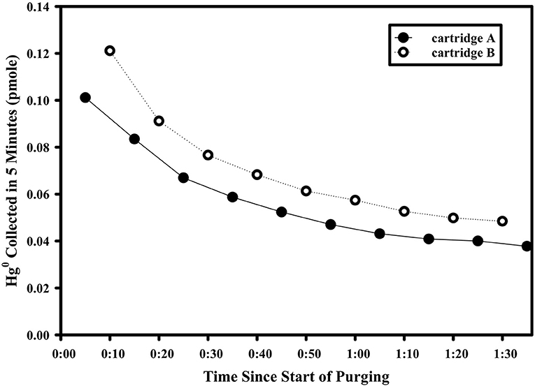
Figure 2. Example time course of the Hg⁰ mass purged from an experimental setup used to determine dark gross reduction rates. These data are from Station 6, with water filtered and taken from 30 m depth.

Incubation Amendments

Away from the surface and a ready source of photons, reactive oxygen species (ROS) and other transient redox species (such as forms of manganese (Mn), iron (Fe), and copper (Cu) as well as biogenic reducing agents) seem the only source of electrons to drive Hg⁰/Hg(II) speciation so far from equilibrium. Furthermore, ROS are generated extracellularly by common marine heterotrophs (Diaz et al., 2013) and within dark marine waters (e.g., Rose et al., 2008b; Zhang et al., 2016), making this suite of compounds worthy of study regarding Hg cycling in dark water. To explore the possible role of ROS in Hg(II) reduction, some gross reduction rate incubations were amended with either hydrogen peroxide (H₂O₂) or nicotinamide adenine dinucleotide (NADH). The first, H₂O₂ is a ROS formed either directly or via dismutation of another ROS species, superoxide (e.g., Blough and Zepp, 1995). The second, NADH, is a reducing equivalent carrier in wide use by bacteria and has been shown to stimulate ROS production both in bacterial culture and natural waters (Andeer et al., 2015; Zhang et al., 2016). Since NADH is only an indirect source of ROS and in case a change in Hg(II) reduction were observed following its addition to our incubations, superoxide dismutase (SOD) was also added to some amendments to act as a control. Superoxide dismutase acts to catalyze the destruction of superoxide to H₂O₂ at seawater pH's (e.g., Kieber et al., 2003). For incubations with H₂O₂ amended, 30% H₂O₂ (ACS grade) was diluted to a secondary stock (50 μM) and then added to the seawater samples to boost the concentration to ~50 or 100 nM. For the superoxide amendments, enough NADH was added to initially raise its concentration to 200 μM through addition of a 5 mM stock solution (MP Biomedicals). For controls with SOD and NADH additions, enough SOD was added to raise the concentration to ~50 kU/L through the use of a 4 kU/mL stock solution (Sigma).

In addition to ROS amendments, some gross reduction incubations were amended with Mn(III) in the form of Mn(III)-DFOB (desferrioxamine-B, as prepared in Madison et al., 2011). Manganese is a well-known redox facilitator in natural waters, but until recently it was thought that only the Mn(II) and Mn(IV) forms were present in environmentally relevant concentrations. There is a growing appreciation, however, that Mn(III), stabilized by organic complexing ligands, can comprise substantial and sometimes majority fractions of dissolved Mn especially in nearshore environments (e.g., Oldham et al., 2017). Thus, we explored whether this redox shuttle might also affect Hg(II) reduction. We added enough Mn(III), bound to desferrioximine-B (DFOB) as a stabilizer, to the incubations to raise the concentration to 500 nM. In addition, and as a control, we added a similar amount of just DFOB to see if affected Hg cycling on it own (presumably through complexation).

Superoxide Concentration Measurements

The in-situ concentration of the superoxide radical (${\text{O}}_2^{·-}$) was measured using the chemiluminescence method described by Rose et al. (2008a), with minor modifications (Sutherland et al., 2020). Superoxide signals were measured by pumping unfiltered seawater (UFSW) or aged filtered seawater (AFSW) from dark bottles using a high accuracy peristaltic pump directly into a flow-through FeLume Mini system (Waterville Analytical, Waterville ME). For AFSW, seawater was filtered (0.2 μm), amended with 50 μM diethylene-triaminepentaacetic acid (DTPA, Sigma), and aged in the dark for at least 8 h in order to eliminate all particle- and metal-associated superoxide (remaining sources would be reactive DOC and/or soluble extracellular enzymes). Superoxide detection was based on the reaction between superoxide and a chemiluminescent probe, a methyl cypridina luciferin analog (MCLA, Santa Cruz Biotechnology; Rose et al., 2008a) as described by Roe et al. (2016). To minimize incidental room light exposure, seawater was pumped into the FeLume using opaque tubing (~20 s transit time between sample bottle and FeLume). For each depth, the superoxide signals were measured within UFSW and AFSW for several minutes (~2–4 min) to achieve a steady-state signal. At the end of each measurement, 800 U L⁻¹ superoxide dismutase (SOD, Sigma) was added to seawater samples. A small fraction of the superoxide signal is a result of reagent auto-oxidation, thus this artifact is removed by taking the difference between two signals as follows. First, the chemiluminescent response, R, in the UFSW and AFSW was quantified relative to the SOD baseline, and converted to concentration using the calibration sensitivity, S_calibration (Equation 1). Next, the total light-independent superoxide concentration was determined using the difference between the UFSW signal and AFSW signal (Equation 2, Roe et al., 2016). The primary assumption here is that the sources of superoxide in the AFSW are negligible; otherwise, the concentrations are underestimates of the true steady-state dark values.

$\begin{array}{ll}{\left[O_2^{·-}\right]}_{(UFSWorAFSW)}=\frac{R_{sample}-R_{sample+SOD}}{S_{calibration}}& (1)\end{array}$

$\begin{array}{ll}{\left[O_2^{·-}\right]}_{total}={\left[O_2^{·-}\right]}_{UFSW}-{\left[O_2^{·-}\right]}_{AFSW}& (2)\end{array}$

Calibrations were conducted using potassium dioxide (Sigma) as detailed previously (Zhang et al., 2016). Briefly, a primary stock solution containing potassium dioxide was prepared and quantified spectrophotometrically (Abs₂₄₀). To prepare the calibration standards, the primary stock solution was further diluted with the calibration matrix to a final superoxide concentration of 5–41 nM. Both primary stock solution and calibration standards were prepared immediately before the analysis. The corresponding chemiluminescent signals were recorded and extrapolated back to the time when the primary standard was quantified, using first order decay kinetics. The half-life of superoxide in AFSW ranged from 0.26 to 0.49 min and the extrapolation time was 0.5–1 min. Calibration curves were constructed based on the linear regression of the natural logarithm extrapolated chemiluminescent signals vs. superoxide concentrations in the calibration standards. Calibrations yielded highly linear curves (e.g., R² > 0.9), with a sensitivity, S_calibration, of 0.16 ± 0.04 (average and standard deviation of different water depths) counts per pM.

Superoxide Production Rate Measurements

At a subset of stations and depths, superoxide decay rates within unfiltered waters were quantified. Decay rate constants of superoxide were determined by spiking in known concentrations of a calibrated potassium dioxide stock at levels ~2–3 times measured in situ concentrations and measuring superoxide decay over time as discussed above. The decay constants were obtained by modeling data using a pseudo-first order decay equation (Shaked and Armoza-Zvuloni, 2013; Armoza-Zvuloni and Shaked, 2014). Waters were spiked with superoxide. Production rates were calculated using the measured steady-state superoxide concentrations and modeled decay rate constants for each water sample (Roe et al., 2016).

Ancillary Measurements

Several ancillary measurements were made using the ship's CTD rosette, including temperature, salinity, dissolved oxygen, chlorophyll fluorescence, beam transmission and photosynthetically active radiation (PAR). The depth of the photic zone was estimated by fitting an exponential curve through the PAR data, and then interpolating to find the depth at 1% of surface irradiance.

Modeling—Formulation

To examine the relative importance of dark and light reduction in Hg⁰ production, we have constructed a relatively simple model of the production of Hg⁰ in the oceanic water column by both light and dark mechanisms. The model seeks to estimate the specific gross rate of Hg⁰ addition in the oceanic mixed layer (the layer in regular contact with the atmosphere and capable of supplying Hg⁰ for evasion).

Assuming first-order kinetics, we modeled the Hg-specific, depth-integrated, gross production of Hg⁰ from Hg(II) using the following equation:

$\begin{array}{l}SIP=\frac{k_{uvb}UVB(1-e^{-{\epsilon }_{uvb}z})}{{\epsilon }_{uvb}}+\frac{k_{par}PAR(1-e^{-{\epsilon }_{par}z})}{{\epsilon }_{par}}\\ +k_{dark}\left(Q_{10}{}^{\frac{T-25}{10}}\right)z& (3)\end{array}$

where SIP is the specific (Hg(II)-normalized) integrated Hg⁰ production, k_uvb and k_par are the photochemical Hg(II) reduction rate constants for UV-B and PAR at the surface (respectively), ε_uvb and ε_par are the exctintion coefficients for UV-B and PAR, k_dark is the reduction rate constant for non-photochemical pathways at 25°C, Q₁₀ is the temperature dependence coefficient of k_dark, z is the depth of the mixed layer and T is the temperature of the mixed layer in °C. The units and values of these terms are summarized in Table 2. Overall, the gross Hg-specific, depth-integrated Hg⁰ production rate has units of meters per day. The first two terms represent the depth-integrated production of Hg⁰ by light-dependent reactions, including abiological photoreduction of Hg(II) complexes by UV-B and the indirect reduction of Hg(II) by phytoplankton during photosynthesis (PAR-dependent term). The rate constants used are those taken from experimental data (Qureshi et al., 2010; Kuss et al., 2015), and assumed to follow an exponential decay in value with depth according to extinction coefficients appropriate for the wavelengths of light involved in those reactions (UV-B for abiological reactions and PAR for biological reactions). The third term is the depth-integrated production of Hg⁰ by dark reactions, assumed to be directly or indirectly related to the activity of heterotrophic microbes. The rate constant here comes from our experiments described above but adjusted for temperature using a Q₁₀ value of 2 (Lee and Fisher, 2019), and which is typical for biological processes. This term might also be expected to have other dependencies related to the activity of bacteria in a given location, including for example primary production. We do not as yet know whether such dependency exists or how to parameterize it and so have left it out. This issue is taken up later as one of the caveats of the model. Temperature within the mixed layer is assumed constant with depth. We could have also included a term for the delivery of Hg⁰ from below the mixed layer as a consequence of vertical eddy diffusion, but initial calculations suggested this term was small enough to ignore. This simplification ignores Hg⁰ produced below the mixed layer that might find its way to the surface following seasonal entrainment (deepening of the mixed layer; e.g., Strode et al., 2007; Soerensen et al., 2010) and is therefore a likely low-end estimate for the rate of Hg⁰ in-growth in the mixed layer. The values used in the equation are summarized in Table 2.

TABLE 2

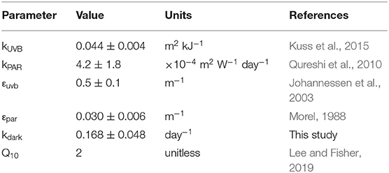
Table 2. Summary of Parameters Used in the Hg⁰ Gross Production Model.

Climatologies for Light, Temperature, and Mixed Layer Depth

To apply these calculations to environmental conditions in different locations, we focused our analyses on 4 months that represent the progression of sunlight and other seasonal conditions (December, March, June, September). We also drew on several publicly available climatologies and recast them in terms of zonal averages over open ocean areas.

The first climatology we used was a two decade long record (1979–2000) of modeled and ground-truthed UV-B irradiances from NCAR (https://www2.acom.ucar.edu/modeling/tuv-download; accessed August 2018, data updated February 2017, Figure S1; Lee-Taylor and Madronich, 2007). This climatology includes the effects of sun angle and attenuation by atmospheric ozone and clouds. As this climatology includes data for UV-B flux to both land and ocean, a land mask was applied to the values prior to calculation of zonal averages and the original latitudinal resolution of 1 degree was converted to 2 degrees. The values provided by the NCAR dataset are presented in units of kJ m⁻² month⁻¹ which we adjusted to kJ m⁻² d⁻¹ for the purposes of comparison to our dark reduction. The UV-normalized, specific Hg(II) reduction rate suggested by Qureshi et al. (2010) was 0.044 ± 0.004 m² kJ⁻¹. We used this value multiplied by the zonally averaged UV-B climatology to get the specific Hg(II) reduction rate (k_uvb, in units of d⁻¹) in surface waters as a function of latitude and time of the year.

The second climatology we incorporated was for PAR so that the contribution of phytoplankton on Hg(II) reduction could be examined. For this purpose, we used downwelling irradiance estimated from the Aqua-MODIS satellite-based radiometer. The data include monthly averages of a time span ~from 2002 to 2017 made available by NASA (https://oceandata.sci.gsfc.nasa.gov/MODIS-Aqua/Mapped/Monthly_Climatology/9km/par), with data updated within the last two years. The original values are served at 9 km resolution which we converted to 2-degree zonal averages, with land values removed. Original units are in einsteins m⁻² s⁻¹, which we transformed to W m⁻² through comparison to NLDAS data to facilitate use with the rate measurements of Kuss et al. (2015). The zonal averages are shown in Figure S4.

The third climatology employed in our model was for global sea surface temperature. These data were retrieved from NCEP (https://ftp.emc.ncep.noaa.gov/cmb/sst/oimonth_v2/) and consisted of combined satellite and in-situ measurements (Reynolds et al., 2002; Figure S5). For use in the model, we assumed that these values were representative of the temperature in the local mixed layer. The original data set was provided in 1-degree resolution, from which we generated 2-degree averages for our analysis.

A fourth climatology applied to our model was that for ocean mixed layer depth developed by de Boyer Montégut et al. (2004), accessed at http://www.ifremer.fr/cerweb/deboyer/mld/home.php and shown in Figure S6. This dataset was provided in 2-degree resolution and was used without further modification.

To compare Hg⁰ production speeds to evasion piston velocities, we also made use of a surface wind speed climatology. We used the Blended Sea Wind product from NOAA, which is the result of NCEP Reanalysis 2 (www.ncdc.noaa.gov/data-access/marineocean-data/blended-global/blended-sea-winds; Zhang et al., 2006). This data set is a monthly climatology making use of data collected from 1995 to 2005 and at 0.25-degree resolution (Figure S7). To appropriately combine with our other datasets, we averaged the data down to 2-degree resolution first, and then generated zonal averages. The zonal average data was then converted to a gas exchange piston velocity using the formula of Wanninkhof (1992), including incorporating modifications for sea surface temperature on the Schmidt Number for Hg⁰ from our zonally average temperature data mentioned above.

Results and Discussion

Species Distributions

The concentration of the Hg species ranged from 0.41 to 2.47 pM for total dissolved Hg and 0.05 to 0.3 pM for Hg⁰, with relatively little variation vertically at the shelf stations (Figure 3). At Station 4 in deeper water, the profile revealed a peak in percent of total Hg as Hg⁰ within the thermocline and below the photic zone. This sort of profile observed at Station 4 is comparable to that observed in other open ocean conditions, where Hg⁰ and percent of total Hg as Hg⁰ often look “nutrient-like” in character, and total Hg to a lesser extent as well (e.g., Bowman, 2014; Bowman et al., 2020). There were no obvious correlations between total Hg, Hg⁰ and percent of total as Hg⁰ and any of the ancillary parameters shown in Figure 3 (temperature, chlorophyll a fluorescence and dissolved oxygen). Dissolved oxygen was never particularly low (range was 192 to 293 μM), though it did tend to decrease below the mixed layer and photic zone. Thus, the concentration of Hg⁰ was always many orders of magnitude above that predicted by equilibrium given the redox properties of the Hg⁰/Hg(II) couple (e.g., Whalin et al., 2007).

FIGURE 3

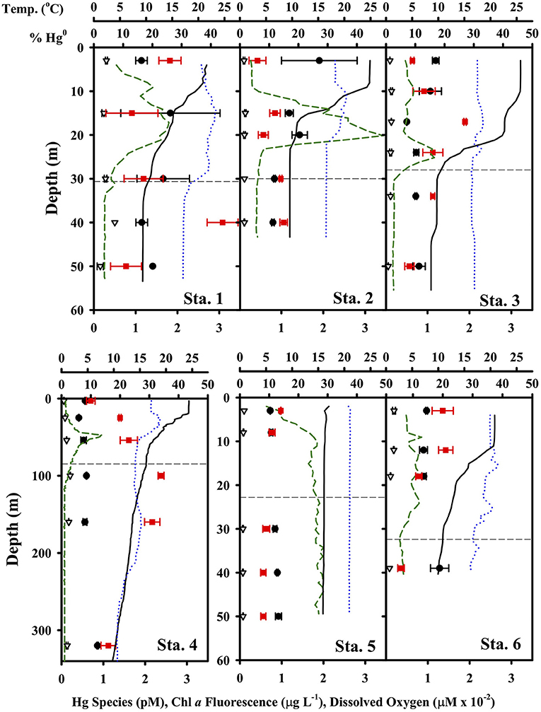
Figure 3. Hg species concentrations and ancillary parameters at each TORCH 2 station. Notice the different depth axis scale for Station 4. In each panel, the black circles are total dissolved Hg, the red circles are percent of total Hg as Hg⁰, the green dashed line is chlorophyll-a fluorescence (in μg/L concentration equivalents), the black line is temperature, and the blue dotted line is dissolved oxygen.

Concentrations of Hg⁰ were supersaturated at all depths and at all stations if the atmospheric concentrations were assumed to be 1.5 ng Hg⁰ m⁻³ (Soerensen et al., 2013) and ranged from 160 to 1,140%. Degrees of supersaturation tended to vary only slightly with depth between about 300 and 400% supersaturation. At shelf stations, the degree of supersaturation was highest in the surface and fell off below the photic zone, while at Station #4 there was a peak in supersaturation just below the photic zone.

Diel Cycling

At two stations, #2 and 6, we conducted diel samplings, where the species were measured at three different depths over the course of 17 and 29 h, respectively (Figure 4). No significant trend in any of the Hg species was observed at these locations over time, suggesting little overall net effect of light on Hg⁰ production. The depths studied included those at the surface (3 m for St. 2 and 6), chlorophyll max (12 and 18 m for St. 6) as well as below the local photic zone (30 and 40 m for St. 2; 39 m for St. 6), and while the concentrations of Hg species were different at the different depths, the temporal trends were the same. These two observations together discourage the view that vertical mixing could have mixed away a photochemical signal making the system appear to have little diel trending. A lack of diel cycling has been noted in other open ocean locations for example by groups using high-resolution underway sampling of Hg⁰ in surface waters (e.g., Andersson et al., 2008; Mason et al., 2017). However, there are studies that have reported diel changes in Hg⁰ concentrations (e.g., Fantozzi et al., 2007; Tseng et al., 2012) and we return to the issue of whether diel cycling should be expected or not below.

FIGURE 4

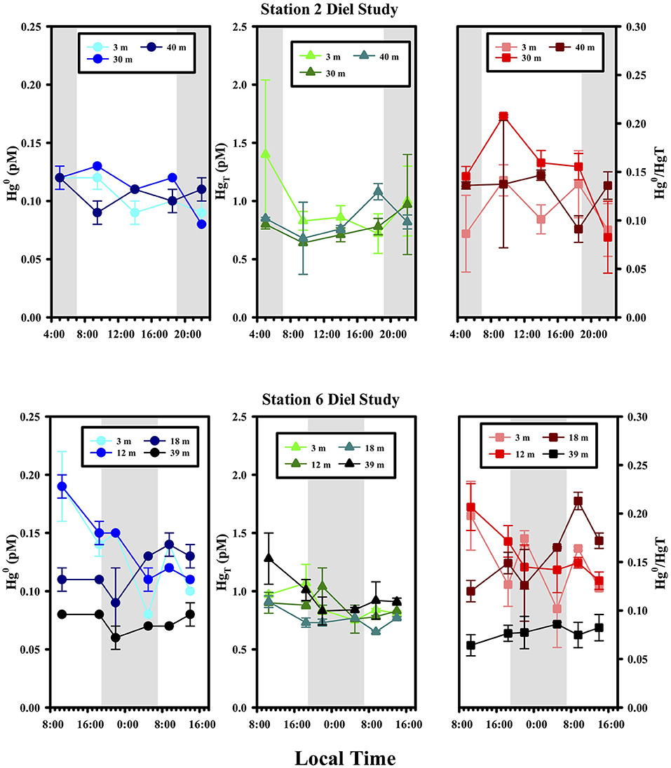
Figure 4. Diel variations of Hg species at Stations 2 and 6. Sunrise and sunset were at ~6:45 and 18:45 local time, respectively.

Gross Reduction Rate Incubations

To begin to probe the underlying mechanisms of Hg reduction, we conducted gross dark reduction incubations in water collected below the photic zone at stations #2, 3, 4 and 6, and depths were 40, 34, 160, and 39 m, respectively. The role of particles was assessed by comparing Hg(II) reduction in unfiltered and filtered waters (Figure 5). The specific gross rate of Hg(II) reduction in unfiltered samples averaged 0.007 ± 0.002 h⁻¹, with no discernible trend among stations. The filtered results were more variable, with the specific rates at Stations #2 and 4 essentially the same as the unfiltered, but at Stations #3 and 6 less than and greater than the unfiltered, respectively. While these results are difficult to interpret, they indicate that filtering does not universally result in a substantial loss of reduction power. Thus, the presence of cells and particulates does not appear necessary for robust dark reduction to take place. Nevertheless, this does not imply that microbes are not involved in dark Hg(II) reduction, but just that reduction can occur without active cells. In fact, we previously observed that Hg(II) reduction in brackish water is facilitated by dissolved compounds that reside in the 3–10 kDa size range (data not shown), which implies the involvement of extracellular enzymes. Thus, it is possible that microbes are required for Hg reduction via the production of dissolved metabolites or extracellular enzymes that promote the reduction reaction.

FIGURE 5

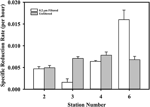
Figure 5. The gross dark specific rate of Hg(II) reduction in filtered and unfiltered water from four TORCH 2 stations. See text for station details.

In addition to the filtered/unfiltered treatments, we also amended a subset of dark gross reduction measurement incubations with chemicals we hypothesized might be involved in promoting or inhibiting Hg reduction. Our initial hypotheses included ones that centered around the potential involvement, either directly or indirectly, of reactive oxygen species including superoxide and hydrogen peroxide. These transient species have redox potentials that lie in the middle of environmentally important redox couples (e.g., Fe, Mn, and Hg) and can therefore variously act as both oxidants and reductants, depending on the compounds with which they are presented. Production of the ROS superoxide (${\text{O}}_2^{·-}$) and hydrogen peroxide (H₂O₂) in natural waters has more recently been attributed in large part to light-independent reactions mediated by particles, presumably composed primarily of microbes (Rose et al., 2008b; Hansard et al., 2010; Roe et al., 2016; Zhang et al., 2016; Sutherland et al., 2020). As these ROS may influence the cycling of Hg, some of our amendment experiments either added exogenous ROS or stimulated ROS production by the resident microbial community.

Figure 6 illustrates the results of amendments made to the seawater in our gross rate incubation experiments designed to explore the influence of ROS. In one set of incubations containing water collected from Station 2 at 40 m, H₂O₂ was added to bring the concentration in the incubation to either 50 or 100 nM. Typical continental shelf waters can be expected to have 10s to 100s of nM H₂O₂ (e.g., Miller and Kester, 1988; Miller et al., 2005). Thus, the amendments were substantial, but within an order of magnitude of the ambient concentrations. The addition of H₂O₂ either had no effect on the gross Hg(II) reduction rate (relative to the unamended control) in the case of unfiltered seawater, or about a 30% decrease in reduction rate in the case of filtered seawater. The absence of any effect in the unfiltered water suggests that the added H₂O₂ was degraded by particles that are presumably microbes. Indeed, the primary pathway of H₂O₂ degradation in the ocean is via microbial enzymatic activity (Moffett and Zafiriou, 1990).

FIGURE 6

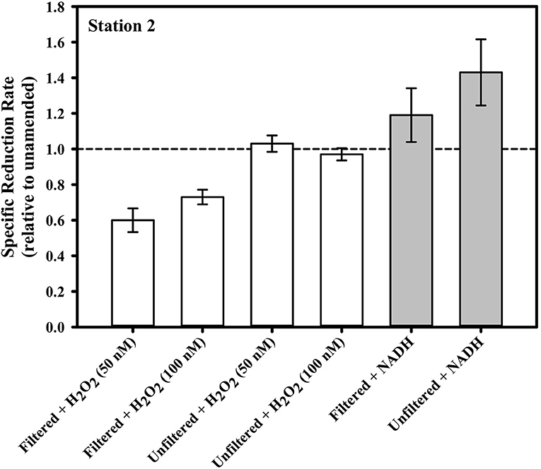
Figure 6. The gross dark specific rate of Hg(II) reduction at Station 2 from water collected at 39 m, with various ROS-related amendments, shown relative to the local unamended control.

Superoxide amendment in the incubations was achieved by stimulating superoxide production via NADH-based enzymes as conducted previously (Zhang et al., 2016). The addition of NADH to both filtered and unfiltered seawater saw a significant change in Hg(II) reduction only in the unfiltered treatment. In that treatment, specific gross reduction increased by about 30% (Figure 6). In a parallel study, laboratory experiments confirmed that NADH does not directly reduce Hg(II) (Marsico, 2015). The results of the two NADH treatments suggest that microbes can be involved in Hg(II) reduction and that this reduction can be stimulated through NADH addition. Including SOD with the NADH treatments (not shown) resulted in no statistically significant loss of the stimulated reduction, implying that the contribution to stimulated reduction activity from superoxide could not be resolved. Consistent with this, if we examine the concentrations of Hg⁰, the ratio of Hg⁰ to total Hg and light-independent steady-state superoxide concentrations from the cruise profiles together (Figure 7), we see no correlation and therefore no circumstantial support for the idea that superoxide contributes to Hg(II) reduction. Furthermore, if we compare the Hg species concentrations and ratios to light-independent superoxide production rates (Figure 7) there appears to be an inverse relationship (at least with the fraction of total as Hg⁰). Therefore, it would seem that superoxide does not contribute to Hg(II) reduction in seawater, or perhaps that under ambient conditions it instead is reacting with some other species which is more influential in Hg(II) reduction.

FIGURE 7

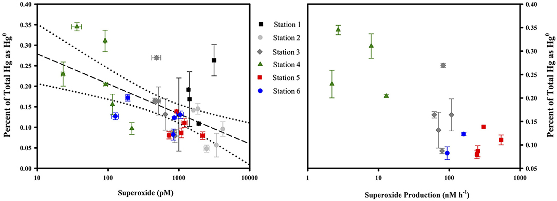
Figure 7. The fraction of total Hg as Hg⁰ compared to the light-independent, steady-state concentration of superoxide (left) and the rate of light-independent superoxide production in unfiltered water (right) at all stations and depths. For more details on the superoxide dynamics (see Sutherland et al., 2020).

Another possible reactant of Hg is oxidized Mn species, including Mn(III)-L complexes. This is particularly interesting in this context because in a parallel study, Mn(III)-L was shown to be abundant within the water column of these sites (Oldham et al., 2020). In the filtered Mn(III)-DFOB amendment incubations, the gross specific rate of reduction jumped by about a factor of 20 relative to filtered but unamended (Figure 8). The filtered+DFOB-only treatment was indistinguishable from the unamended, suggesting the dramatic increase in Hg reduction was the result of the presence of the Mn(III), not DFOB, in solution. Interestingly, when the same pair of Mn(III)-DFOB and DFOB-only treatments were applied to unfiltered seawater, there was only a modest increase in the gross reduction rate when Mn(III) was present, and a decrease in the gross rate when DFOB alone was present. This suggests that when cells were present, the DFOB may have facilitated cell uptake of Hg(II) or otherwise rendered the Hg(II) in a form that was not available for reduction. When both Mn(III) and DFOB were present along with cells, the two apparent competing forces of increased reduction from the Mn vs. the sequestration from the DFOB+cell combination resulted in an increase in reduction that was modest.

FIGURE 8

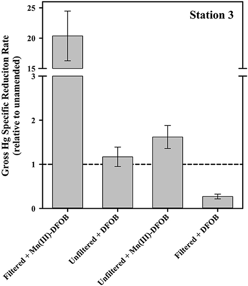
Figure 8. The gross dark specific rate of Hg(II) reduction at Station 3 with Mn(III)-related amendments, shown relative to the local unamended control.

As noted above, there was no discernible trend in the gross specific rate of Hg(II) reduction in unfiltered samples across our stations. This is interesting because the stations where our experiments were conducted include waters with a range in cell abundance from 0.4·10⁶ to 2·10⁶ bacterial cells mL⁻¹ in aphotic waters (Sutherland et al., 2020) and perhaps a range in community activity as well. This suggests three possibilities: (1) Hg(II) reduction in the dark is not dependent on heterotrophic bacterial activity at all and whatever the agent responsible for Hg reduction was, had a uniform distribution or was at sufficient excess at all our stations, (2) cells at the lower abundance site had a higher per cell dark reduction rate than cells at the higher abundance sites, or (3) the rate of dark reduction, whatever the mechanism, is set by a slow step other than the reaction itself, for example the rate of release of Hg from a “hard-to-reduce” pool.

The gross specific rate measured here is also interesting in that it is slower than photochemical reduction, but still relatively fast. The dark rates we observed were similar to those reported earlier (e.g., Whalin et al., 2007), though perhaps better resolved. Thus, even in open ocean conditions and as suggested by others for coastal environments, depth-integrated dark reduction has the potential to provide more Hg⁰ in the mixed layer than light reactions under conditions where the mixed layer depth is relatively deep.

Zonally Averaged Modeling

To explore the hypothesis that depth-integrated dark reduction can be more important that light reduction, we used the model described above, driven with climatological data to get an estimate for the total, depth-integrated production rate of Hg⁰ within the mixed layer and the apportionment of that production between light-dependent and -independent (dark) mechanisms. The results from these calculations are shown in Figure 9 and summarized in Table 3. Several features of the model output are worth discussing. First, the overall rate of reduction varies dramatically with latitude, with tropical regions producing Hg⁰ at a much faster specific rate than high latitude regions. Furthermore, as tropical latitudes make up a larger fraction of the ocean's area than do high latitudes, the model predicts that the tropical ocean is where the majority of Hg reduction takes place. This does not necessarily translate into higher evasional fluxes, however, as re-oxidation rates and wind speed will influence the specific rate of evasion. For example, as Kuss et al. (2011) noted, relatively high concentrations of Hg⁰ can be found in tropical surface waters, but winds at these latitudes tend to be lower than at higher latitudes. Thus, they found maximal evasion fluxes (per unit area) in temperate waters.

FIGURE 9

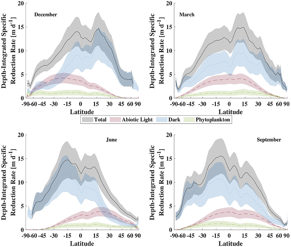
Figure 9. Comparison of the zonal-averaged depth-integrated Hg specific reduction rate for representative months, in units of meters per day. The lines are the mean value while the shaded areas are the ± 1 standard deviation envelope.

TABLE 3

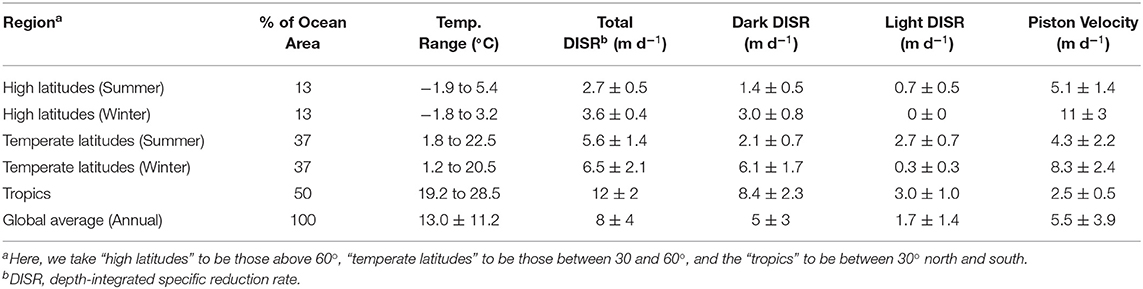
Table 3. Model result summary.

The second major feature of the output to notice is that integrated dark specific reduction is faster than either of the light-dependent pathways, as well as the sum of the two, except in high and temperate latitudes during local summer. The abiological (photochemical) light reduction pathway is everywhere greater than the phytoplankton pathway as well. Therefore, the model predicts that temperature, which is the primary control on dark reduction, is the critical modulator of Hg⁰ specific production and explains why warm tropical waters dominate global specific reduction. In addition to high specific reduction, the tropics also experience high loadings of Hg(II) to the ocean from their relatively high precipitation depths, which when combined to vigorous reduction, leads to high Hg⁰ concentrations and high evasion rates in and around the intertropical convergence zone (Kuss et al., 2011; Soerensen et al., 2013, 2014; He and Mason, 2020).

Comparing the residence times of Hg⁰ in the mixed layer with respect to reduction/oxidation and evasion reveals that in most locations oxidation is a bigger gross sink for Hg⁰ from the mixed layer than is evasion. Figure 10 portrays this by calculating the ratio of the residence time of Hg⁰ with respect to evasion, divided by the residence time with respect to production from Hg(II):

$\begin{array}{ll}R=\frac{k_{red}[Hg(II)]ML}{k_{piston}[H{g}^0]}& (4)\end{array}$

where k_red is the overall reduction rate constant, ML is the depth of the mixed layer, and k_piston is the gas exchange piston velocity. In Figure 10, the ratio of Hg⁰ to Hg(II) in the mixed layer is assumed to be 0.5 everywhere, which is undoubtedly an overestimate for most locations, but which means that the ratio is likely larger in most places. As the value is much larger than one under most conditions, this implies that oxidation of Hg⁰ is a larger sink than evasion and therefore the steady-state concentration of Hg⁰ is set by redox cycling more or less independently of the strength of evasion. As evasion is driven in part by the dissolved Hg⁰ concentration, this in turn implies that evasion rates are driven by the balance between oxidation and dark reduction, and not gross reduction rates. Figure 10 suggests that the speeds of redox and evasion approach each other at high latitudes allowing evasion to remove more of the Hg⁰ after it is produced and before it can be oxidized. Under these conditions, it is possible for the speed of gross reduction to be more influential on evasion rates. As reduction rates are their highest in warm water with a shallow mixed layer, we should expect high latitudes in the summer hemispheres to exhibit relatively large net fluxes of Hg⁰ and possibly see diel cycling if mixed layer depths are shallow.

FIGURE 10

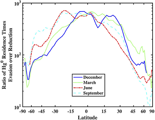
Figure 10. Comparison of the zonal-averaged depth-integrated Hg specific reduction rate (in units of meters per second) and piston velocity (k value in the gas-exchange model, also in units of meters per second).

Modeling Caveats

One potential weakness of this modeling approach is the oversimplified view of the ocean mixed layer. A truly well-mixed surface layer is one with uniformly short residence times at all depths and is required in our model to justify our mathematical arguments described above. However, Franks (2014) pointed out that while a layer of uniform properties like temperature and salinity might be identified from data, this is an imperfect proxy for a surface turbulent layer in which the residence time at any one depth is truly short. Franks summarized several forces that can contribute to turbulence and true mixing, and found that only two, convection and Langmuir circulation, are capable of providing turbulence and mixing deeper than a few meters. While these two forces can act at any time and result in relatively rapid mixing, they tend to occur discontinuously and are more important in the evening, in cooler seasons, and under strong and steady winds. Thus, our use of the mixed layer climatology of de Boyer Montegut et al. could overestimate the depth of turbulent mixing on any given day, and may even have some diel and seasonal bias as well. This could be tested by looking for any temporal trends in the various high resolution surface Hg⁰ data sets that are becoming more common (Andersson et al., 2011; Soerensen et al., 2014; Mason et al., 2017; DiMento et al., 2019). Some observers using more conventional datasets have already reported seeing diel trends. For example, Tseng and colleagues reported trends in the South China Sea, as did Fantozzi et al. in the Mediterranean and DiMento et al. in the Arctic (Fantozzi et al., 2009; Tseng et al., 2013; DiMento et al., 2019). But as we noted in our own data (see Figure 4), this is far from universal. Therefore, we suggest that when the depth of real mixing, as opposed to the conventional definition we've used here, is deeper than the “critical depth” for Hg reduction (the depth at which integrated dark reduction equals integrated light reduction and analogous to the concept in primary production; Franks, 2014), dark reduction will dominate Hg⁰ production and observers will see little evidence of diel cycling. This would imply that those cases where diel cycles have been observed were therefore situations where the depth of real mixing was shallower than the critical depth.

A second important caveat to this model is that we have assumed a temperature dependence to dark Hg reduction on the basis that the production of reducing equivalents in the dark almost certainly has to be biological in nature. Assuming this is true, then all the various factors that affect dark biological Hg reduction should also be included. One of the most important is likely to be primary production within the photic zone, as this is the source of fixed carbon to bacteria that may be reducing Hg. However, we have not attempted to include primary production as a variable in our model because we simply lack information on how this might affect Hg reduction. Our prediction is that greater bacterial production should increase Hg reduction, though our range of studies did not seem to bear this out. Assuming it is true, however, then dark Hg reduction might be expected to have a spatial trend similar to that of phytoplankton-driven Hg reduction. If this were true, then it would suggest that our model currently overestimates Hg reduction in the winter hemisphere at mid-latitudes, where production is relatively low but temperatures are warm. We do not believe this will change the overall conclusion that dark reduction dominates in most places, but this is clearly an important topic for further research.

Implications

The combination of measurement and modeling presented here argues that dark reduction, rather than light-driven reduction, is responsible for most of the Hg⁰ produced in and evaded from the global surface ocean. As this reduction produces concentrations of Hg⁰ that are dramatically out of equilibrium, they must be actively supported by a ready supply of reducing agents that are likely of biological origin. This implies that factors affecting the activity of marine heterotrophs within the mixed layer can subsequently affect the production and evasion of Hg⁰ from the ocean. Such factors include temperature and primary productivity, both of which are likely to change in the future and in ways that are hard to predict. For example, warming should stimulate heterotrophic activity and could enhance primary productivity (e.g., Behrenfeld, 2011), both of which should enhance Hg evasion according to our results. But warming would also result in a shoaling of the mixed layer and restriction of new production, both of which should decrease the importance of dark biological reduction. More study of the temperature and biological sensitivies of Hg redox are needed to make predictions regarding the future of the marine Hg cycle.

Data Availability Statement

The datasets presented in this study can be found in online repositories. The names of the repository/repositories and accession number(s) can be found at: https://www.bco-dmo.org/dataset/765327/data.

Author Contributions

CL, CH, and BV designed the experiments. All authors contributed to data collection and writing.

Funding

This work was supported by NSF Grant OCE-1355720 (to CH, CL, and BV).

Conflict of Interest

The authors declare that the research was conducted in the absence of any commercial or financial relationships that could be construed as a potential conflict of interest.

Acknowledgments

Thanks to the captain and crew of the R/V Endeavor, as well as the science crew of the TORCH2 cruise, with special thanks to Alison Agather, Lindsey Starr, and Bill Fanning. Thanks to Mak Saito, Brian Guest, and the Winch Pool staff at WHOI for sampling equipment assistance. Thanks to Asif Qureshi, Joachim Kuss, Mathis Hain, and Jessica McCarty for data sharing, help with remote sensing data and data presentation advice. Thanks to Jerome Fietcher for discussion of mixed layers. Thanks also the insightful comments of two reviewers.

Supplementary Material

The Supplementary Material for this article can be found online at: https://www.frontiersin.org/articles/10.3389/fenvc.2021.659085/full#supplementary-material

Figure S1. Sea surface temperature (°C) in the NW Atlantic at the time of TORCH 2 cruise as collected by the MODIS instrument on the Aqua satellite. The figure depicts average values from 9/17/2017 to 9/23/2017.

Figure S2. Concentration of chlorophyll-a (mg L⁻¹) in the NW Atlantic at the time of TORCH 2 cruise as collected by the MODIS instrument on the Aqua satellite. The figure depicts average values from 9/17/2017 to 9/23/2017.

Figure S3. Zonal-averaged surface UV-B flux in units of kJ m⁻² d⁻¹ for representative months.

Figure S4. Zonal-averaged surface photosynthetically active radiation (PAR; units of kJ m⁻² d⁻¹) flux for representative months.

Figure S5. Zonal-averaged sea surface temperature in degrees Celsius for representative months.

Figure S6. Zonal-averaged mixed layer depth in meters for representative months.

Figure S7. Zonal-averaged surface winds in meters per second for representative months.

References

Andeer, P. F., Learman, D. R., McIlvin, M., Dunn, J. A., and Hansel, C. M. (2015). Extracellular haem peroxidases mediate Mn (II) oxidation in a marine Roseobacter bacterium via superoxide production. Environ. Microbiol. 17, 3925–3936. doi: 10.1111/1462-2920.12893

PubMed Abstract | CrossRef Full Text | Google Scholar

Andersson, M. E., Gardfeldt, K., and Wangberg, I. (2008). A description of an automatic continuous equilibrium system for the measurement of dissolved gaseous mercury. Anal. Bioanal. Chem. 391, 2277–2282. doi: 10.1007/s00216-008-2127-4

PubMed Abstract | CrossRef Full Text | Google Scholar

Andersson, M. E., Sommar, J., Gardfeldt, K., and Jutterstrom, S. (2011). Air-sea exchange of volatile mercury in the North Atlantic Ocean. Mar. Chem. 125, 1–7. doi: 10.1016/j.marchem.2011.01.005

CrossRef Full Text | Google Scholar

Armoza-Zvuloni, R., and Shaked, Y. (2014). Release of hydrogen peroxide and antioxidants by the coral Stylophora pistillata to its external milieu. Biogeosciences 11, 4587–4598. doi: 10.5194/bg-11-4587-2014

CrossRef Full Text | Google Scholar

Behrenfeld, M. (2011). Uncertain future for ocean algae. Nat. Clim. Chang. 1, 33–34. doi: 10.1038/nclimate1069

CrossRef Full Text | Google Scholar

Blough, N. V., and Zepp, R. G. (1995). “Reactive oxygen species in natural waters,” in Active Oxygen in Chemistry, eds C. S. Foote, J. S. Valentine, A. Greenberg, and J. F. Liebman (Dordrecht: Springer Netherlands), 280–333.

PubMed Abstract | Google Scholar

Bowman, K. L. (2014). Mercury Distributions and Cycling in the North Atlantic and Eastern Tropical Pacific Oceans. Dayton, OH: Wright State University.

Google Scholar

Bowman, K. L., Lamborg, C. H., and Agather, A. M. (2020). A global perspective on mercury cycling in the ocean. Sci. Tot. Environ. 710:136166. doi: 10.1016/j.scitotenv.2019.136166

PubMed Abstract | CrossRef Full Text | Google Scholar

Costa, M., and Liss, P. S. (1999). Photoreduction of mercury in sea water and its possible implications for Hg-0 air-sea fluxes. Mar. Chem. 68, 87–95. doi: 10.1016/S0304-4203(99)00067-5

CrossRef Full Text | Google Scholar

de Boyer Montégut, C., Madec, G., Fischer, A. S., Lazar, A., and Iudicone, D. (2004). Mixed layer depth over the global ocean: an examination of profile data and a profile-based climatology. J. Geophys. Res. Oceans 109:C12003. doi: 10.1029/2004JC002378

CrossRef Full Text | Google Scholar

Diaz, J. M., Hansel, C. M., Voelker, B. M., Mendes, C. M., Andeer, P. F., and Zhang, T. (2013). Widespread production of extracellular superoxide by heterotrophic bacteria. Science 340, 1223–1226. doi: 10.1126/science.1237331

PubMed Abstract | CrossRef Full Text | Google Scholar

DiMento, B. P., Mason, R. P., Brooks, S., and Moore, C. (2019). The impact of sea ice on the air-sea exchange of mercury in the Arctic Ocean. Deep Sea Res. Pt. I Oceanogr. Res. Pap. 144, 28–38. doi: 10.1016/j.dsr.2018.12.001

CrossRef Full Text | Google Scholar

Fantozzi, L., Ferrara, R., Frontini, F. P., and Dini, F. (2007). Factors influencing the daily behaviour of dissolved gaseous mercury concentration in the Mediterranean Sea. Mar. Chem. 107, 4–12. doi: 10.1016/j.marchem.2007.02.008

CrossRef Full Text | Google Scholar

Fantozzi, L., Ferrara, R., Frontini, F. P., and Dini, F. (2009). Dissolved gaseous mercury production in the dark: evidence for the fundamental role of bacteria in different types of Mediterranean water bodies. Sci. Tot. Environ. 407, 917–924. doi: 10.1016/j.scitotenv.2008.09.014

PubMed Abstract | CrossRef Full Text | Google Scholar

Franks, P. J. S. (2014). Has Sverdrup's critical depth hypothesis been tested? Mixed layers vs. turbulent layers. ICES J. Mar. Sci. 72, 1897–1907. doi: 10.1093/icesjms/fsu175

CrossRef Full Text | Google Scholar

Hansard, S. P., Vermilyea, A. W., and Voelker, B. M. (2010). Measurements of superoxide radical concentration and decay kinetics in the Gulf of Alaska. Deep Sea Res. Pt. I Oceanogr. Res. Pap. 57, 1111–1119. doi: 10.1016/j.dsr.2010.05.007

CrossRef Full Text | Google Scholar

He, Y. P., and Mason, R. P. (2020). “Comparison of air-sea exchange of mercury from the GEOTRACES GP15 cruise with data from other cruises in the Pacific Ocean: from similarity to discrepancy,” in Ocean Sciences (San Diego, CA: American Geophysical Union).

Google Scholar

Johannessen, S. C., Miller, W. L., and Cullen, J. J. (2003). Calculation of UV attenuation and colored dissolved organic matter absorption spectra from measurements of ocean color. J. Geophys. Res. Oceans 108:13. doi: 10.1029/2000JC000514

CrossRef Full Text | Google Scholar

Kieber, D. J., Peake, B. M., and Scully, N. M. (2003). Reactive oxygen species in aquatic. UV Effects Aquat. Organ. Ecosyst. 1:251. doi: 10.1039/9781847552266-00251

CrossRef Full Text | Google Scholar

Kuss, J., Wasmund, N., Nausch, G., and Labrenz, M. (2015). Mercury emission by the baltic sea: a consequence of cyanobacterial activity, photochemistry, and low-light mercury transformation. Environ. Sci. Technol. 49, 11449–11457. doi: 10.1021/acs.est.5b02204

PubMed Abstract | CrossRef Full Text | Google Scholar

Kuss, J., Zülicke, C., Pohl, C., and Schneider, B. (2011). Atlantic mercury emission determined from continuous analysis of the elemental mercury sea-air concentration difference within transects between 50°N and 50°S. Global Biogeochem. Cycles 25:GB3021. doi: 10.1029/2010GB003998

CrossRef Full Text | Google Scholar

Lamborg, C. H., Hammerschmidt, C. R., Gill, G. A., Mason, R. P., and Gichuki, S. (2012). An intercomparison of procedures for the determination of total mercury in seawater and recommendations regarding mercury speciation during GEOTRACES cruises. Limnol. Oceanogr. Methods 10, 90–100. doi: 10.4319/lom.2012.10.90

CrossRef Full Text | Google Scholar

Lamborg, C. H., Tseng, C. M., Fitzgerald, W. F., Balcom, P. H., and Hammerschmidt, C. R. (2003). Determination of the mercury complexation characteristics of dissolved organic matter in natural waters with “reducible Hg” titrations. Environ. Sci. Technol. 37, 3316–3322. doi: 10.1021/es0264394

PubMed Abstract | CrossRef Full Text | Google Scholar

Lee, C. S., and Fisher, N. S. (2019). Microbial generation of elemental mercury from dissolved methylmercury in seawater. Limnol. Oceanogr. 64, 679–693. doi: 10.1002/lno.11068

PubMed Abstract | CrossRef Full Text | Google Scholar

Lee-Taylor, J., and Madronich, S. (2007). Climatology of UV-A, UV-B, and erythemal radiation at the Earth's surface, 1979-2000. Boulder, CO: NCAR Technical Note NCAR/TN-474+STR, NCAR.

Google Scholar

Madison, A. S., Tebo, B. M., and Luther, I. I. I. G. W. (2011). Simultaneous determination of soluble manganese (III), manganese (II) and total manganese in natural (pore) waters. Talanta 84, 374–381. doi: 10.1016/j.talanta.2011.01.025

PubMed Abstract | CrossRef Full Text | Google Scholar

Marsico, R. M. (2015). Implications of Widespread Dark Production and Decay of Reactive Oxygen Species in Natural Waters. Golden, CO: Colorado School of Mines.

Google Scholar

Mason, R. P., Hammerschmidt, C. R., Lamborg, C. H., Bowman, K. L., Swarr, G. J., and Shelley, R. U. (2017). The air-sea exchange of mercury in the low latitude Pacific and Atlantic Oceans. Deep Sea Res. Pt. I Oceanogr. Res. Pap. 122, 17–28. doi: 10.1016/j.dsr.2017.01.015

CrossRef Full Text | Google Scholar

Miller, G. W., Morgan, C. A., Kieber, D. J., King, D. W., Snow, J. A., Heikes, B. G., et al. (2005). Hydrogen peroxide method intercomparision study in seawater. Mar. Chem. 97, 4–13. doi: 10.1016/j.marchem.2005.07.001

CrossRef Full Text | Google Scholar

Miller, W. L., and Kester, D. R. (1988). Hydrogen peroxide measurement in seawater by (p-hydroxyphenyl)acetic acid dimerization. Anal. Chem. 60, 2711–2715. doi: 10.1021/ac00175a014

CrossRef Full Text | Google Scholar

Moffett, J., and Zafiriou, O. (1990). An investigation of hydrogen peroxide chemistry in seawater by isotope ratio mass spectrometry using 18O2 and H218O2. Limnol. Oceanogr. 35, 1221–1229.

Morel, A. (1988). Optical modeling of the upper ocean in relation to its biogenous matter content (case I waters). J. Geophys. Res. Oceans 93, 10749–10768. doi: 10.1029/JC093iC09p10749

CrossRef Full Text | Google Scholar

O'Driscoll, N. J., Siciliano, S. D., Lean, D. R. S., and Amyot, M. (2006). Gross photoreduction kinetics of mercury in temperate freshwater lakes and rivers: application to a general model of DGM dynamics. Environ. Sci. Technol. 40, 837–843. doi: 10.1021/es051062y

PubMed Abstract | CrossRef Full Text | Google Scholar

Oldham, V. E., Lamborg, C. H., and Hansel, C. M. (2020). The spatial and temporal variability of Mn speciation in the coastal Northwest Atlantic Ocean. J. Geophys. Res. Oceans 125:e2019JC015167. doi: 10.1029/2019JC015167

CrossRef Full Text | Google Scholar

Oldham, V. E., Mucci, A., Tebo, B. M., and Luther, G. W. III (2017). Soluble Mn(III)-L complexes are abundant in oxygenated waters and stabilized by humic ligands. Geochim. Cosmochim. Acta 199, 238–246. doi: 10.1016/j.gca.2016.11.043

CrossRef Full Text | Google Scholar

Outridge, P. M., Mason, R. P., Wang, F., Guerrero, S., and Heimbürger-Boavida, L. E. (2018). Updated global and oceanic mercury budgets for the United Nations Global Mercury Assessment 2018. Environ. Sci. Technol. 52, 11466–11477. doi: 10.1021/acs.est.8b01246

PubMed Abstract | CrossRef Full Text | Google Scholar

Qureshi, A., O'Driscoll, N. J., MacLeod, M., Neuhold, Y. M., and Hungerbuhler, K. (2010). Photoreactions of mercury in surface ocean water: gross reaction kinetics and possible pathways. Environ. Sci. Technol. 44, 644–649. doi: 10.1021/es9012728

PubMed Abstract | CrossRef Full Text | Google Scholar

Reynolds, R. W., Rayner, N. A., Smith, T. M., Stokes, D. C., and Wang, W. (2002). An improved in situ and satellite SST analysis for climate. J. Clim. 15, 1609–1625. doi: 10.1175/1520-0442(2002)015andlt;1609:AIISASandgt;2.0.CO;2

CrossRef Full Text | Google Scholar

Roe, K. L., Schneider, R. J., Hansel, C. M., and Voelker, B. M. (2016). Measurement of dark, particle-generated superoxide and hydrogen peroxide production and decay in the subtropical and temperate North Pacific Ocean. Deep Sea Res. Pt. I Oceanogr. Res. Pap. 107, 59–69. doi: 10.1016/j.dsr.2015.10.012

CrossRef Full Text | Google Scholar

Rolfhus, K. R. (1998). The production and distribution of elemental hg in a coastal marine environment [Ph.D.dissertation]. University of Connecticut, Stamford, CT, United States.

Google Scholar

Rolfhus, K. R., and Fitzgerald, W. F. (2004). Mechanisms and temporal variability of dissolved gaseous mercury production in coastal seawater. Mar. Chem. 90, 125–136. doi: 10.1016/j.marchem.2004.03.012

CrossRef Full Text | Google Scholar

Rose, A. L., Moffett, J. W., and Waite, T. D. (2008a). Determination of superoxide in seawater using 2-Methyl-6-(4-methoxyphenyl)-3,7- dihydroimidazo[1,2-a]pyrazin-3(7H)-one c chemiluminescence. Anal. Chem. 80, 1215–1227. doi: 10.1021/ac7018975

PubMed Abstract | CrossRef Full Text | Google Scholar

Rose, A. L., Webb, E. A., Waite, T. D., and Moffett, J. W. (2008b). Measurement and implications of nonphotochemically generated superoxide in the equatorial Pacific Ocean. Environ. Sci. Technol. 42, 2387–2393. doi: 10.1021/es7024609

PubMed Abstract | CrossRef Full Text | Google Scholar

Shaked, Y., and Armoza-Zvuloni, R. (2013). Dynamics of hydrogen peroxide in a coral reef: sources and sinks. J. Geophys. Res. Biogeosci. 118, 1793–1801. doi: 10.1002/2013JG002483

CrossRef Full Text | Google Scholar

Soerensen, A. L., Mason, R. P., Balcom, P. H., Jacob, D. J., Zhang, Y., Kuss, J., et al. (2014). Elemental mercury concentrations and fluxes in the tropical atmosphere and ocean. Environ. Sci. Technol. 48, 11312–11319. doi: 10.1021/es503109p

PubMed Abstract | CrossRef Full Text | Google Scholar

Soerensen, A. L., Mason, R. P., Balcom, P. H., and Sunderland, E. M. (2013). Drivers of surface ocean mercury concentrations and air–sea exchange in the west atlantic ocean. Environ. Sci. Technol. 47, 7757–7765. doi: 10.1021/es401354q

PubMed Abstract | CrossRef Full Text | Google Scholar

Soerensen, A. L., Sunderland, E. M., Holmes, C. D., Jacob, D. J., Yantosca, R. M., Skov, H., et al. (2010). An improved global model for air-sea exchange of mercury: high concentrations over the North Atlantic. Environ. Sci. Technol. 44, 8574–8580. doi: 10.1021/es102032g

PubMed Abstract | CrossRef Full Text | Google Scholar

Strode, S. A., Jaegle, L., Selin, N. E., Jacob, D. J., Park, R. J., Yantosca, R. M., et al. (2007). Air-sea exchange in the global mercury cycle. Glob. Biogeochem. Cycles 21:GB1017. doi: 10.1029/2006GB002766

CrossRef Full Text | Google Scholar

Sutherland, K. M., Coe, A., Gast, R. J., Plummer, S., Suffridge, C. P., Diaz, J. M., et al. (2019). Extracellular superoxide production by key microbes in the global ocean. Limnol. Oceanogr. 64, 2679–2693. doi: 10.1002/lno.11247

CrossRef Full Text | Google Scholar

Sutherland, K. M., Grabb, K. C., Karolewski, J. S., Plummer, S., Farfan, G. A., Wankel, S. D., et al. (2020). Spatial heterogeneity in particle associated dark superoxide production within productive coastal waters. J. Geophys. Res. Oceans 125:e2020JC016747. doi: 10.1029/2020JC016747

CrossRef Full Text | Google Scholar

Tseng, C. M., Lamborg, C. H., and Hsu, S. C. (2013). A unique seasonal pattern in dissolved elemental mercury in the South China Sea, a tropical and monsoon-dominated marginal sea. Geophys. Res. Lett. 40, 167–172. doi: 10.1029/2012GL054457

CrossRef Full Text | Google Scholar

Tseng, C. M., Liu, C. S., and Lamborg, C. (2012). Seasonal changes in gaseous elemental mercury in relation to monsoon cycling over the northern South China Sea. Atmos. Chem. Phys. 12, 7341–7350. doi: 10.5194/acp-12-7341-2012

CrossRef Full Text | Google Scholar

Wanninkhof, R. (1992). Relationship between wind-speed and gas-exchange over the ocean. J. Geophys. Res. Oceans 97, 7373–7382. doi: 10.1029/92JC00188

CrossRef Full Text | Google Scholar

Whalin, L., Kim, E. H., and Mason, R. (2007). Factors influencing the oxidation, reduction, methylation and demethylation of mercury species in coastal waters. Mar. Chem. 107, 278–294. doi: 10.1016/j.marchem.2007.04.002

CrossRef Full Text | Google Scholar

Zhang, H., and Lindberg, S. E. (2001). Sunlight and iron(III)-induced photochemical production of dissolved gaseous mercury in freshwater. Environ. Sci. Technol. 35, 928–935. doi: 10.1021/es001521p

PubMed Abstract | CrossRef Full Text | Google Scholar

Zhang, H.-M., Bates, J. J., and Reynolds, R. W. (2006). Assessment of composite global sampling: sea surface wind speed. Geophys. Res. Lett. 33:L17714. doi: 10.1029/2006GL027086

CrossRef Full Text | Google Scholar

Zhang, T., Hansel, C. M., Voelker, B. M., and Lamborg, C. H. (2016). Extensive dark biological production of reactive oxygen species in brackish and freshwater ponds. Environ. Sci. Technol. 50, 2983–2993. doi: 10.1021/acs.est.5b03906

PubMed Abstract | CrossRef Full Text | Google Scholar