The Effect of Particle Composition and Concentration on the Partitioning Coefficient for Mercury in Three Ocean Basins

Introduction

Removal of trace elements by particle scavenging has a first-order control on their concentrations in the ocean (Anderson, 2014). This is true for mercury (Hg) as well: particle scavenging represents the ultimate sink for Hg from the ocean over centuries, and it is eventually back to the deep mineral reservoir on the timescales of glacial cycle (e.g., Amos et al., 2013). At present, the global burial flux for Hg in ocean sediments is not very well-constrained but likely lies between the value of 1.2 μg m⁻² y⁻¹ in open ocean conditions and 1,200 μg m⁻² y⁻¹ in hyper-accumulating regions like the Antarctic margin (Soerensen et al., 2016; Zaferani et al., 2018). Models have suggested that the global burial flux falls between 1.7 and 7 μg m⁻² y⁻¹ (e.g., Outridge et al., 2018; Tesán Onrubia et al., 2020). Given the current oceanic inventory of Hg, these burial fluxes suggest a residence time of Hg of about 520 years (Outridge et al., 2018).

Mercury likely finds its way from solution onto suspended and sinking particles via processes that John and colleagues have called “regenerative scavenging” (John and Conway, 2014; Lamborg et al., 2016). This mechanism is unlike that exhibited by trace elements such as thorium, for which reversible partitioning appears to occur and results in steady-state particle-/aqueous-phase ratios that are dependent on the composition of the particulate phase (Bacon and Anderson, 1982; Chase et al., 2002; Hayes et al., 2015). In regenerative scavenging, some irreversible process such as biological uptake in surface waters is responsible for the movement of an element from the solution- to the particle-phase initially, and the return reaction is only accomplished when the particles themselves are altered or destroyed, forcing the trace elements (and macro-material) back into solution followed by re-association with the altered particles. A combination of non-reversible and reversible processes broadly describes the nature of all “hybrid-type” elements and thus we should expect that their distribution in and removal from the ocean to be controlled by regenerative scavenging. To best understand and describe such cycling, we would benefit from a study of the kinetics of sorption, desorption, uptake, and remineralization as has been done for thorium (e.g., Lerner et al., 2018). However, unlike for thorium, sources of Hg are not well-known making a mass balance inverse approach more difficult, and we are therefore forced to rely on some proxy information to guide our understanding. The empirical distribution coefficient (K_d) is one such proxy and has been used extensively in modeling studies for a variety of elements (e.g., Honeyman and Santschi, 1989). However, in the case of Hg it has been noted that the value of K_d remains poorly constrained (Zhang et al., 2014). We recently examined the magnitude and variability of K_d of Hg in the Atlantic Ocean using data generated from the U.S. GEOTRACES and found that K_d values were substantially higher than had been assumed in the past and that the particle phase with the strongest apparent affinity for Hg was manganese oxide (MnO₂), followed by iron oxyhydroxide [Fe(OH)₃], particulate organic matter (POM), calcium carbonate (CaCO₃), and lithogenic particles in decreasing order (Lamborg et al., 2016). However, as the oxide phases represented only a small fraction of total particulate mass (0.8% for iron and 0.1% for manganese), their apparent contribution to overall Hg sorption (if indeed Hg is to be found in marine particles as a result of sorption) was modest. Instead, POM was the most important phase with its sorption fraction at 36%, CaCO₃ next at 30%, and lithogenic phase at 29%. These findings supported the generally held hypothesis that POM is highly influential in determining the phase distribution of Hg in the environment (Fitzgerald and Lamborg, 2014). However, it also suggested that the influence of POM is not exclusive and perhaps not even responsible for the majority of Hg partitioned to the particle phase. In this manuscript, we extended the Lamborg et al. (2016) Atlantic examination to two additional basins including the eastern tropical South Pacific Ocean and the Western Arctic Ocean. We also subject the datasets to additional statistical analyses in search of a predictive model of Hg phase partitioning. The analysis here makes use of total dissolved and particulate Hg but could be performed on monomethylmercury as well. The contributions of monomethylmercury to total dissolved and particulate Hg are relatively small and so were not removed prior to our calculations. Therefore, the K_d values derived using total Hg values are close approximations for the Hg(II) form.

Methods

Data Used

All datasets used here are from U.S. GEOTRACES cruises, including the East Pacific zonal transect (nickname EPZT; GEOTRACES transect number GP16, cruise identifier TN303), the North Atlantic zonal transect (NAZT, GA03; KN199-04 and KN204-1), and the Western Arctic (GN01; HLY1502). We used data from 58 stations in total with 22 in the Pacific, 17 in the Atlantic and 19 stations in the Arctic Ocean (Figure 1). All data used were from the BCO-DMO data repository.

FIGURE 1

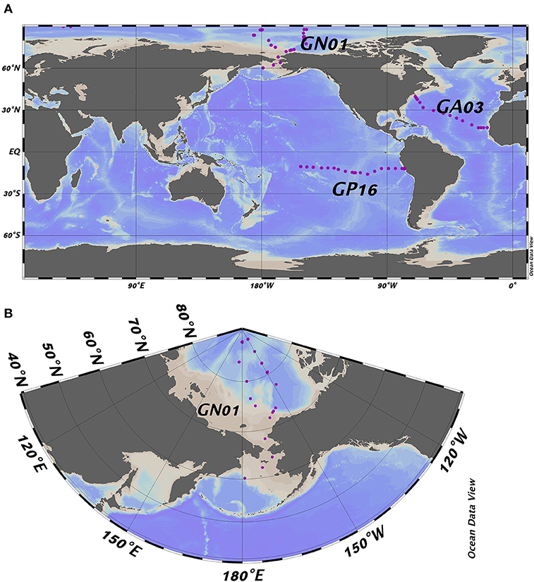
Figure 1. (A) Full map of the three GEOTRACES cruises including GP16, GA03, and GN01; (B) Zoomed in map of GN01. Purple dots represent the location of the sampling stations referred to in the text.

The Hg data have all been published previously, with the dissolved and particulate total mercury data from Agather et al. (2019) (GN01) and Bowman et al. (2015, 2016) (GA03 & GP16). The published particle mass and composition data are from Lam et al. (2015, 2018), Xiang and Lam (2020). Due to lack of access to large-size-fraction (>51 μm; LSF) samples for Hg analysis, we only used small-size-fraction (1–51 μm; SSF) particle composition and particulate Hg data in our mercury partition coefficient analysis. Note that the original collected data are linked with “flags” indicating the data quality, in order to have convincing results, we made sure that all parameters we used were identified as either “good” (Quality Flag = 2) or “possibly good” (QF = 3) quality at the same depth.

Partition Coefficient (K_d) Analysis

Here, the partition coefficient (K_d) is defined as the apparent affinity of mercury for marine particles. This concept was inspired from studies of Bacon et al. (1976) and Baskaran and Santschi (1993). K_d is calculated as:

$\begin{array}{ll}{K}_d=\frac{C_p}{C_d}\times \frac{1}{SPM}& (1)\end{array}$

where C_p and C_d represent the concentration of Hg in particulate and dissolved phases, respectively, and SPM is the suspended particulate mass (kg L⁻¹). This results in K_d having units of volume per mass, conventionally as L kg⁻¹. Here C_d represents the concentration passing a 0.2-μm filter and therefore includes both dissolved and colloidal Hg. Particle sampling depths at each station were not exactly the same as the dissolved phase, thus, to calculate partition coefficients, we estimated concentrations of the dissolved phase by linear interpolation (using the MATLAB routine “interp1”) to the depths of particle phase samples.

In order to better understand how bulk partition coefficients relate to particle composition, a six-end member mixing model was applied, which is similar to the one developed by Hayes et al. (2015) for thorium isotopes. The contribution of each major particle phase to the measured bulk K_d is represented by the following formula:

$\begin{array}{l}{K}_d={\displaystyle \sum _1^6}{(K_d)}_i·f_i={(K_d)}_1·f_1+{(K_d)}_2·f_2+{(K_d)}_3·f_3\\ +{(K_d)}_4·f_4+{(K_d)}_5·f_5+{(K_d)}_6·f_6& (2)\end{array}$

where K_d is the observed bulk partition coefficient, (K_d)_i is the apparent partition coefficient for pure phase i, f_i is the fraction of certain particle phase i over particulate mass, and I = 1(POM), 2(CaCO₃), 3(Opal), 4(lithogenic), 5(MnO₂), 6(Fe(OH)₃). The (K_d)_i, which we and Hayes call the intrinsic K_d, was calculated using non-negative least-squares regression (“lsqnonneg”) in MATLAB for individual basin datasets, as well as some sub-basin datasets:

$\begin{array}{ll}\left[\begin{array}{cccccc}{f}_1^1& f_2^1& f_3^1& f_4^1& f_5^1& f_6^1\\ f_1^2& f_2^2& f_3^2& f_4^2& f_5^2& f_6^2\\ f_1^3& f_2^3& f_3^3& f_4^3& f_5^3& f_6^3\\ ⋮& ⋮& ⋮& ⋮& ⋮& ⋮\\ f_1^N& f_2^N& f_3^N& f_4^N& f_5^N& f_6^N\end{array}\right]\times \left[\begin{array}{c}{(K_d)}_1\\ {(K_d)}_2\\ {(K_d)}_3\\ ⋮\\ {(K_d)}_6\end{array}\right]=\left[\begin{array}{c}{K}_d^1\\ K_d^2\\ K_d^3\\ ⋮\\ K_d^N\end{array}\right]& (3)\end{array}$

To estimate the standard error of the derived intrinsic K_d values, we used the jackknife re-sampling technique suggested by Hayes et al. (2015) and Efron and Stein (1981).

Principal Component Analysis of Bulk K_d and Particle Composition

We performed PCA on the partition coefficient and particle composition data to see if a few principal components (PCs), or linear combinations of the original variables, could explain a large proportion of the total variance in dataset being considered. Therefore, PCA was conducted on the following seven variables: bulk log K_d, f_POM, f_CaCO3, f_opal, f_lithogenic, f_MnO2, f_Fe(OH)3, in order to analyze the relationship between bulk K_d and particle composition fraction among three different ocean basins. Since the units and magnitude of the 7 variables are different, prior to PCA the sample data were mean-centered and normalized by standard deviation (“zscore” function in MATLAB). The PCA itself was performed using the MATLAB function “pca”. In addition, we constructed biplots of loadings and scores associated with PC's 1 and 2 to visualize the results, which interprets the correlation for each of the original variables as well as the direction of increasing values.

Principal Component Analysis of Residual K_d and Particle Composition

We did linear regression to model the relationship between SPM and bulk K_d. The residuals K_d data were calculated as the vertical distance in the Y-axis between each data point and the fitted line and represent the portion of K_d not explained by SPM. Following the same data processing strategy as in section Principal Component Analysis of bulk K_d and particle composition, we performed PCA on the residuals and particle composition data to examine whether this would better reveal a particle composition effect.

Results and Discussion

In this section, we present our data results and employ a model to demonstrate the particle concentration and composition effect on Hg partitioning. In addition to discussion on some special features of K_d, we extended the study of K_d on Hg residence time at the end.

Dissolved and Particulate Hg Profiles

The mean and median concentrations of dissolved and particulate total mercury for the three ocean basins were calculated in the surface (above 100 m), as well as every 500 m depth in the deep water (below 100 m; Figure 2). Overall, the concentration of dissolved Hg in the Arctic was the highest (around 1.1 pM) at the surface, as a result of riverine input, atmospheric deposition and ice melt (e.g., Fitzgerald et al., 2005; Agather et al., 2019), and decreased to ~0.5 pM at depth. In contrast, the dissolved Hg in the Pacific and Atlantic Ocean was distributed in a more nutrient-like way, characterized by a slight increasing trend with depth. Note that there was a maximum at 3,500 m in the Atlantic is due to the influence of the TAG hydrothermal vent where total dissolved Hg increased to 13 pM.

FIGURE 2

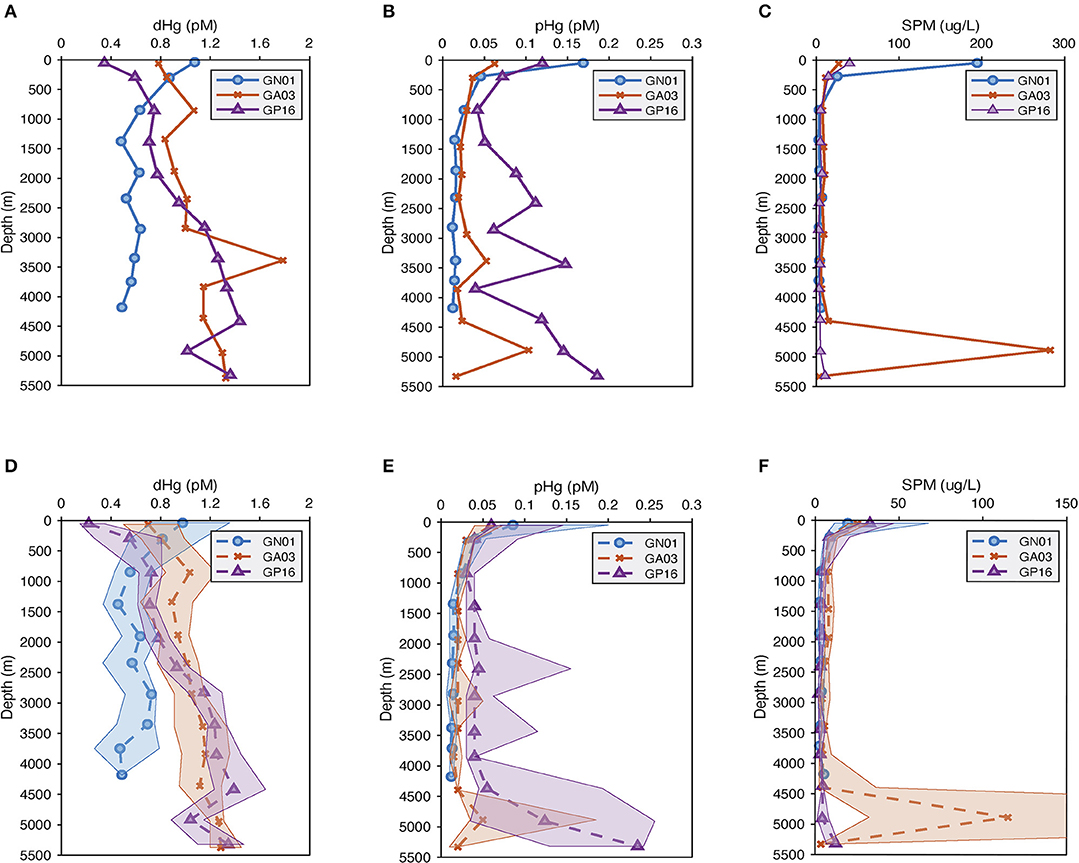
Figure 2. (A–C) are average vertical profiles of dissolved and particulate Hg (pM) as well as suspended particulate matter (SPM) (μg/L) from three US GEOTRACES cruises; while (D–F) are median vertical profiles of dissolved and particulate Hg (pM) as well as suspended particulate matter (SPM) (μg/L), and the shade is 25 to 75 percentiles for the median plots.

The particulate Hg started with the highest concentration at the surface in all basins, attenuating quickly below the photic zone and reaching the minimum at about 1,000 m. In the Pacific Ocean, a strong hydrothermal plume led to abnormally high concentrations of particulate Hg in deep water (between 2,500 and 3,500 m), accompanied by high variability as well. Similarly, the SPM concentration in the three ocean basins attenuated with depth. At the surface, the mean SPM concentration in the Arctic was around 6 times greater than that in the Pacific and Atlantic, resulting from the extremely high SPM over the continental shelf (Xiang and Lam, 2018). The median surface SPM concentration in the Arctic was the lowest of the three basins, however, reflecting the very oligotrophic Canadian Basin in the Western Arctic Ocean (Xiang and Lam, 2020). A maximum occurred in the deep ocean of the Atlantic due to the influence of strong bottom nepheloid layers in the Deep Western Boundary Current (Lam et al., 2015).

Bulk Partition Coefficient (K_d) for the Three Ocean Basins

Bulk partition coefficient values varied widely over the whole dataset, ranging in order from 10⁴ to 10⁸ L kg⁻¹ (Figure 3). In the Pacific, the bulk partition coefficients were extremely high, with an average order of magnitude of 10⁷ (range: 5.05 × 10⁵-1.63 × 10⁸ L kg⁻¹; log K_d = 5.70–8.21). The bulk K_d values from the Atlantic, in contrast, were lowest and ranged from 2.60 × 10⁵ to 6.73 × 10⁷ L kg⁻¹ (log K_d = 5.41–7.83). Compared to these two ocean basins, the K_d value from the Arctic Ocean were modestly lower and ranged from 9.70 × 10⁴ to 6.99 × 10⁷ L kg⁻¹ with an average on the order of 10⁶. Summary K_d statistics are presented in Supplementary Table 1. As previously noted by Lamborg et al. (2016), these K_d values are substantially higher than those previously reported for freshwaters, sediment porewaters over continental shelves (~10⁴ L kg⁻¹) (e.g., Hammerschmidt and Fitzgerald, 2004) and coastal waters (10⁵-10⁶ L kg⁻¹) (e.g., Balcom et al., 2008).

FIGURE 3

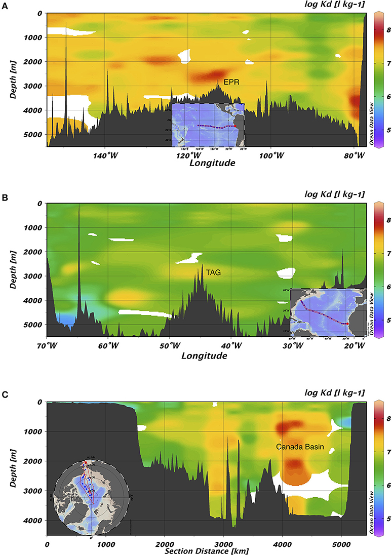
Figure 3. Section views of log Kd (L kg⁻¹) values in (A) GP16, (B) GA03, and (C) GN01. The highest value on average was found in the Pacific, while the lowest on average was found in the Atlantic. EPR represents East Pacific Rise; TAG represents Trans-Atlantic Geotraverse hydrothermal field located on Mid-Atlantic Ridge.

Intrinsic K_d

End-member coefficients, or intrinsic K_d, were calculated for each of the six particle phases in the SSF in all three cruises, including POM, CaCO₃, opal, lithogenic, Mn oxides, and Fe oxyhydroxides. The value of intrinsic K_d and composition fractions are summarized in Table 1. Overall, the intrinsic K_d values varied between ocean basins. One commonality, however, was that the intrinsic K_d for opal could not be defined using this method in any of the three ocean basins. The intrinsic K_d for POM, CaCO₃, and lithogenic phases could always be estimated, but had different values. As for Fe and Mn, the contribution to sorption of Hg could be evident when their concentrations were high, typically observed in hydrothermal vents. Otherwise, their influence on Hg partitioning was negligible.

TABLE 1

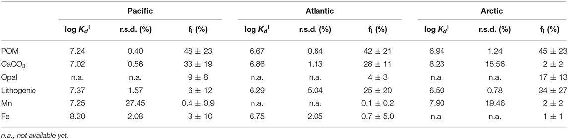
Table 1. The log intrinsic ${\text{K}}_{\text{d}}^{\text{i}}$ (l kg⁻¹) of Hg for six particle composition in the small size fraction (SSF) in the Pacific, Atlantic, and Arctic ocean, respectively, and their relative standard deviation (r.s.d.) as well as particle composition mass contribution (f; %).

If there is really is such a thing as an “intrinsic K_d” that expresses the stickiness of Hg to a measured particle phase, the calculated values should be homogeneous everywhere in the ocean. However, an examination of our results suggests that this might not be true. We applied the Z-test based on intrinsic K_d values and their standard deviations (Table 1), setting the confidence interval to 95%, to test whether the intrinsic K_d values for each particle phase were significantly different between basins. Generally speaking, intrinsic K_d between ocean basins were similar for some phases but significantly different for others. For instance, intrinsic K_d values of POM in three ocean basins were significantly different (P < 0.05). In contrast, the values for CaCO₃ of three ocean basins were statistically indistinguishable (P > 0.05). This suggests that the precise composition of POM with respect to its ability to scavenge Hg varies between ocean basins but that CaCO₃ does not (or varies less). Since the three cruises were sampled in different seasons and different environments, the dominant plankton were likely not the same in the three ocean basins, and the components of collected POM presumably varied with different plankton. The intrinsic K_d of the lithogenic phase in the Arctic Ocean was different from those in the Pacific and Atlantic Oceans. This is perhaps not surprising, since “lithogenic particles” is a category that represents a diverse range of aluminosilicate minerals, which might be expected to have different sorption characteristics for Hg (e.g., Biscaye, 1965; Darby, 1975). Interestingly, intrinsic K_d values of Mn had no significant difference (P > 0.05) in the Pacific and Arctic Ocean, while intrinsic K_d values of Fe were significantly different (P < 0.05) between the Pacific and the Atlantic Ocean. The Fe intrinsic K_d differences between basins implies a qualitative difference in the Fe itself, but this remains to be explored.

PCA of Hg Partitioning and Particle Composition

The PCA results are summarized in Table 2, which includes 7 variables (the bulk K_d value and the fraction of the six particle fractions), loadings of the first three principal components (PC) and their contribution in explaining the total variance. In the East Pacific, the first three principal components explained 77.64% of variation of the seven variables with 35.33% explained by PC1, 22.78% explained by PC2, and 19.53% explained by PC3. The highest loadings for PC1 were the fractions of Fe and Mn, both of which were positively correlated with bulk K_d, which could result from the hydrothermal plume (Lam et al., 2018). For PC2, the relative fractions of POM had strong positive loadings, while f_CaCO3, f_litho, and f_opal were negatively loaded, which means the organic matter was anticorrelated with minerals. This negative correlation reflects the variation in depth: decreasing POM and increasing lithogenic particles with depth (Lam et al., 2018). The fractions of CaCO₃ and opal were strongly anticorrelated in PC3 (Table 2, Figure 4), which might reflect the variation of region: higher opal in the coastal region, abundant CaCO₃ in the open ocean (Lam et al., 2018). In the Atlantic, 63.85% of total variance was explained by the first three components with 30.56% explained by PC1, 17.64% explained by PC2, and 15.65% explained by PC3. Based on our observations, in PC1, bulk K_d and the fractions of POM were anticorrelated with fractions of lithogenic particles and Mn, reflecting the depth variation of POM and lithogenic particles (Lam et al., 2015). For PC2, the fraction of CaCO₃ was strongly correlated with bulk K_d, and for PC3 the fractions of opal were anticorrelated with Fe and Mn. Additionally, the first three principal components of the Arctic dataset explained 77.92% of the total variance, where PC1 explained 39.15%, PC2 explained 35.61%, and PC3 explained 13.16%. The highest loadings of PC1 were observed from the fractions of lithogenic particles and POM, which could be the consequence of variations in depth and/or region (Xiang and Lam, 2020), whereas PC2's highest loadings were mainly from bulk K_d, and the fractions of Mn, CaCO₃ and opal. The f_CaCO3 and f_Mn were positively correlated with bulk K_d while f_opal was negatively correlated with bulk K_d. PC3's highest loadings were the fractions of Mn, CaCO₃ and opal which were positively correlated with each other.

TABLE 2

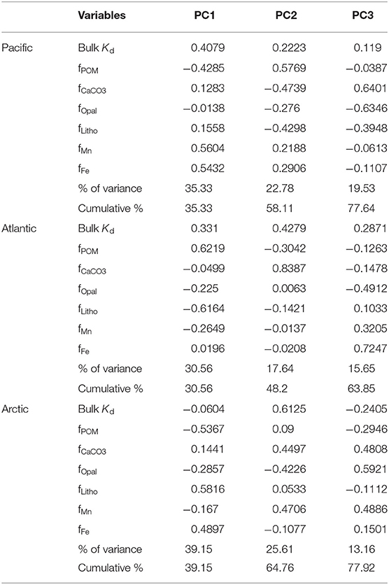
Table 2. The first three principal component loadings, percentage of variance explained by each principal component, and their cumulative percentage of total variance including bulk K_d and six particle compositions in the small size fraction of particles.

FIGURE 4

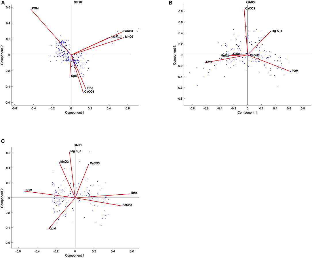
Figure 4. Biplots of principal component (PC1 and PC2) for the (A) GP16, (B) GA03, and (C) GN01, respectively. The red lines represent loadings for each variable; blue dots represent the scores for each observation.

From the biplots of scores and loadings (Figure 4), the K_d loadings were strongest with PC1 in the Pacific, and PC2 in the Atlantic and Arctic. As already noted above, PC1 in the Pacific was most strongly associated with Fe and Mn oxides, implying a significant influence of those phases on the overall value of K_d. This is likely due to the influence of hydrothermal Fe- and Mn-rich particles sorbing Hg from seawater. In the Atlantic and Arctic, PC2 was also strongly loaded with CaCO₃, and relatively poorly loaded for POM, implying a major role of CaCO₃ in Hg sorption in those basins, but less of a role for POM.

Furthermore, the biplots loadings (Figure 4) for each ocean basins suggested that the PC1 and PC2 could be driven by different variables. The significant strong positive loadings in PC1 for both Mn, Fe and bulk K_d in the Pacific imply that this PC was related to some natural processes that affected bulk K_d in a similar manner with Mn and Fe in the Pacific. Similarly, PC2 has strong positive loadings for Mn and bulk K_d in the Arctic also suggested these two variables behaves similarly and closely correlated with each other, since the high absolute and relative concentrations of manganese oxides were observed in the Arctic halocline and deep water, leading to strong scavenging of various elements (Xiang and Lam, 2020). However, there is no significant correlation between f_MnO2 and log K_d in the Atlantic, suggesting that f_MnO2 can't be the only control on log K_d globally. Meanwhile, f_MnO2 is very low in the Atlantic, possibly accounting for its little influence in scavenging Hg.

Particle Concentration and Composition Effects on Partition Coefficient

Particle Concentration Effect

We began our investigation of the potential drivers of K_d by examining the effect of particle concentration on the partitioning of Hg. The linear regression model in Figure 5 shows the relationship between log SPM (μg L⁻¹) and log bulk K_d (L kg⁻¹) for the three ocean basins. A significant inverse correlation was observed in all basins, which is consistent with the findings reported by Moran et al. (1996). Similar inverse relationships were observed between log K_d of ²¹⁰Pb and ²¹⁰Po and SPM in these transects (Tang et al., 2017; Bam et al., 2020). The inverse relationship between K_d and SPM, also known as “the particle concentration effect” (Honeyman et al., 1988), can be explained by at least three mechanisms. The first one centers around the effects of colloidal chemistry on metal distributions within the particulate phase (e.g., Honeyman and Santschi, 1989; Benoit and Rozan, 1999; Bam et al., 2020). Assuming Hg species sorb to colloids and as colloids are too small to be collected by conventional filtration, GEOTRACES sampling methods tend to count colloids as “dissolved” and thereby result in a smaller K_d value for Hg than the ideal circumstance when colloids are properly accounted for in the particle pool. Furthermore, the proportion of colloids over the particulate mass is generally thought to increase with SPM concentrations, leading to a negative K_d vs. SPM slope (Moran et al., 1996). Indeed, based on two observed relationships between colloidal and SPM concentrations, Moran et al. (1996) modeled the percent of colloidal Hg on the particle mass and found that it tends to increase with SPM concentrations if SPM are <10⁴ μg L⁻¹. A second possibility is that particle mass is not a good proxy for available particle surface sorption sites for Hg. The material reported here as SPM at a specific location is made up of many individual particles that vary in size, with the number of small particles generally being much greater than the number of large particles (e.g., Stemmann and Boss, 2012). Particle size distributions vary between different samples, and therefore each SPM sample has varying proportions of large and small constituents. Samples in high productivity regions with high SPM can also be expected to have a relatively high proportion of large particles (e.g., diatom cells), while low SPM samples are more prevalent in oligotrophic regions where cells are mostly small (e.g., picoplankton). Thus, we might expect that the smaller the SPM is, the more Hg scavenged by a given particle mass as a consequence of larger surface area-to-volume ratios for smaller particles. As area-to-volume ratios scale with the inverse of particle size, one might predict that a bulk K_d vs. SPM plot should resemble an inverse curve. However, no discernible trend between the total SPM concentration (Total SPM = SSF SPM + LSF SPM) and fSSF, the mass fraction of small particles over total particles (fSSF = SSF SPM/Total SPM) during the same cruises, was evident (Figure 6). The fSSF is an analog to the slope of the particle mass-size spectrum (Xiang et al., 2020) or the number-size spectrum (e.g., Cael and White, 2020), a higher fSSF implies more abundance of small particles. Hence, it is likely that the particle size did not change with SPM concentrations in particles. Therefore, the “particle-size hypothesis” appears unsupported by these datasets. A third possibility for the apparent particle concentration effect is a kinetic explanation. The ratio of the adsorption to desorption rate constant, normalized by SPM, can be thought of, in some circumstances, as a kinetic representation of K_d (Honeyman et al., 1988). In a kinetic study of the adsorption and desorption of thorium, both the adsorption and desorption rate constants were found to increase with SPM, but at different rates, such that their ratio normalized by SPM also decreased with SPM, much like the classic particle concentration effect (Lerner et al., 2017). Although this kinetic explanation for the apparent particle concentration effect has so far only been observed for thorium, it is a potential alternative to explain the particle concentration effect that does not rely on colloids. This then leaves the influence of colloids, and perhaps the kinetics of particle attachment and detachment, as the possible explanations for the K_d vs. SPM trends observed in our data.

FIGURE 5

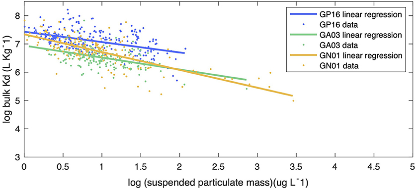
Figure 5. The linear regression between log bulk Kd (l kg⁻¹) and particle concentration (log SPM in ug l⁻¹) in the small size fraction for Pacific (blue line), Atlantic (green line), and Arctic (yellow line) oceans. The slopes of linear regression for each ocean basins were −0.367, −0.423, −0.629, with statistics R-squared equals 0.2155, 0.2218, 0.5338, respectively. The slope of the Arctic was significantly different from the slopes of the Pacific and the Atlantic by applying Z-test, with statistics P < 5%.

FIGURE 6

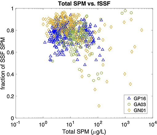
Figure 6. Scatter plot between Total SPM concentrations (unit: μg/L) and the fraction of SSF particles (fSSF) in all three cruises. The Total SPM is calculated as SSF SPM+ LSF SPM, and the fSSF as SSF SPM/Total SPM.

Particle Composition Effect

Additionally, we argue that variations in bulk K_d also partly result from the particle composition effect. The decreasing trend in bulk K_d with SPM (Figure 5) clearly shows the influence of SPM, but the variations around this trend are still worth being investigated. We assumed this variation is from particle composition. Different statistical methods were employed to obtain the information about the impact of particle composition on partition coefficient.

In some specific regions, the value of bulk K_d was clearly driven by the SPM concentration. For example, high concentrations of SPM in the deep water of the western Atlantic (Lam et al., 2015) corresponded to low bulk K_d. Similarly, the Arctic continental shelf also had abundant SPM (Xiang and Lam, 2020), coinciding with low bulk K_d values. At the other end of the SPM spectrum, high K_d values were found in Arctic mid-waters where SPM was low. This was not universally true, however, as demonstrated by much higher bulk K_d in relatively low SPM water in the Canada Basin in the Western Arctic Ocean. We take this to be evidence of another factor that influences the bulk K_d, namely the particle composition effect. This effect is described by the intrinsic K_d values in each basin and which can be better understood by multiplying the mean compositional fraction for each particle phase by the intrinsic K_d we calculated (Figure 7). The corresponding value, when compared to those of other phases, expresses the relative importance for each phase in sorbing Hg from solution (if that kind of chemistry does in fact occur). The resulting pie charts indicate that for these three oceans, POM and CaCO₃ dominate Hg partitioning. This trend holds across all the basins despite there being large variations in the abundance of CaCO₃ as a result of compensatory changes in the intrinsic K_d for that phase (Table 1). Moreover, the contributions of lithogenic material to bulk K_d were also quite similar in the three oceans, with percentages from 9 to 11%, while the fraction of it was distinct everywhere.

FIGURE 7

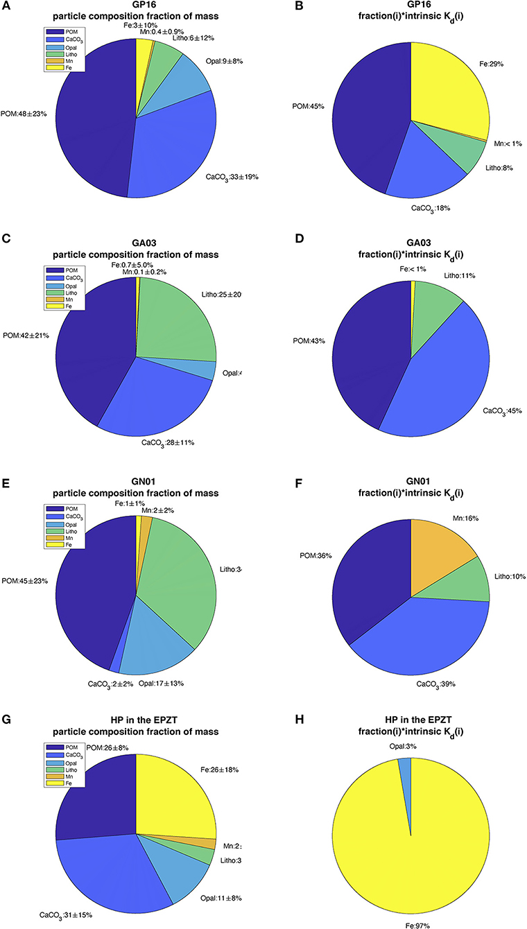
Figure 7. The pie charts (A,C,E,G) described the mean and standard deviation of particle composition fraction of mass in the Pacific (GP16), Atlantic (GA03), Arctic (GN01), and hydrothermal plume in EPZT; chart (B,D,F,H) described the mean proportion of each composition fraction multiplying their intrinsic Kd in four regions above, respectively.

It is worth noting that Fe contributions to bulk K_d were quite variable and were high only in the Pacific, caused by relatively high Fe fraction in particles released in a hydrothermal plume. Similarly, the abundant Mn observed in the Arctic also accounted for a large part of the bulk K_d. Therefore, we can see that Mn and Fe had strong adsorption affinities to Hg in some regions despite their relatively low concentration level in particles. The strong sorption affinity of Mn is apparently not only for Hg but also to ²³⁴Th, ²³¹Pa, ²¹⁰Po, and ²¹⁰Pb (Hayes et al., 2015; Lerner et al., 2018; Bam et al., 2020). As noted above and discussed below, there was no resolvable intrinsic K_d value for opal and so it does not appear in the pie charts of Figure 7. This implies that opal plays a minor role in the partitioning of Hg into the particle phase, at least in these three basins.

In Figure 5, bulk K_d data from the three oceans were scattered around the regression lines with SPM. We examine the hypothesis that the residuals to the SPM relationship, which are the vertical distance between each data point and the regression lines, might be explained by particle composition. Hence, we applied PCA to see the relationship between residuals of log K_d and particle phases. The PCA results are presented in Supplementary Table 2. In the Pacific, the highest loadings for PC1 were the fractions of Fe and Mn, which were positively associated; for PC2, POM, CaCO₃ and the residuals had the highest loadings, where POM correlated positively with residuals whereas CaCO₃ correlated negatively with residuals. Information from PC1 suggests that POM was also a crucial factor that led to the variance of K_d in the Atlantic; CaCO₃ had a positive association with residuals in the Arctic from PC2.

Besides PCA, we applied the least squares regression of particle composition fraction to the K_d residuals of the SPM regression, which we called the “intrinsic residual K_d” ($K_{\text{d}}^{*}$) (Table 3).

$\begin{array}{l}residuals={\displaystyle \sum _1^6}{(K_d^{*})}_i·f_i={(K_d^{*})}_1·f_1+{(K_d^{*})}_2·f_2+{(K_d^{*})}_3·f_3\\ +{(K_d^{*})}_4·f_4+{(K_d^{*})}_5·f_5+{(K_d^{*})}_6·f_6& (4)\end{array}$

In general, the particle composition explained the 39.72% of variance of residuals in the Pacific Ocean, 6.25% of variance of residuals in the Atlantic Ocean and 12.88% of variance of residuals in the Arctic Ocean. In the Pacific, Mn and Fe had a strong correlation with residuals compared with other particle phases. Mn could result in lower K_d while Fe contributed to a higher K_d. CaCO₃ and lithogenic particles have little effect in driving bulk K_d to be lower than the regression line (Figure 5), while POM has a positive feedback on bulk K_d. In the Atlantic, POM, CaCO₃, lithogenic phase and Fe lead to positive residuals that makes bulk K_d higher above the fitting line (Figure 5). Additionally, POM, lithogenic phase have strong positive correlation with residuals in the Arctic, while Mn led to smaller K_d values in the Arctic.

TABLE 3

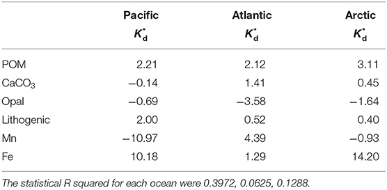
Table 3. The coefficients to the least squares regression of the residual ${\text{K}}_{\text{d}}^{*}$ (L kg⁻¹) of Hg for six particle composition fractions (Equation 4) in the small size fraction (SSF) in the Pacific, Atlantic, and Arctic ocean, respectively.

By adding R-squared values that are generated from the linear regression model of SPM and K_d (Figure 5) to R-squared values from least squares regression above, we could have a general view of how much variation of partition coefficient that can be demonstrated by both particle concentration and composition effect. Overall, the SPM combined particle composition explained the 61.27% of variance of K_d in the Pacific, 28.43% of variance of K_d in the Atlantic, and 66.26% of variance of K_d in the Arctic. However, these values were possibly overestimated, since SPM and composition effect are not completely independent in our model. Despite that residuals to the SPM regression remove the effect of particle concentration which represents a pure composition effect on K_d, the regression of log K_d against SPM carries some particle composition effect information which we don't know how to eliminate so far.

Special Features: Hydrothermal Plume and Coast

Part of the reason for the exceptionally high K_d values observed from the EPZT cruise dataset was the presence of high Fe at stations/depths associated with the continental shelf and East Pacific Rise hydrothermal plume. Thus, we separated the EPZT data into three subsets based on the dissolved Fe concentrations reported by Resing et al. (2015), including a coastal margin (stations 1–5), hydrothermal vents (stations 18, 20, 21, 25, 26, where depth was between 2,200 and 3,000 m) and open ocean (the rest of stations and depths). The bulk K_d values for the coastal margin subset were lower than the average (between 5.05 × 10⁵ to 7.84 × 10⁷ L kg⁻¹; log K_d = 5.70–7.89), whereas higher than average bulk K_d value were observed in hydrothermal vent subset (from 1.26 × 10⁷ to 1.63 × 10⁸ L kg⁻¹; log K_d = 7.10–8.21). The bulk K_d value of the open ocean subset was between 1.92 × 10⁶ and 8.85 × 10⁷ L kg⁻¹ (log K_d = 6.28–7.95). The intrinsic K_d values in each subset are summarized in Table 4. Interestingly, the pattern of intrinsic K_d values was very different between these three regions, similarly resulted from what we discussed in section Intrinsic K_d. In the coastal data subset, only carbonate and lithogenic particle fractions were able to explain bulk K_d variability and in the hydrothermally influenced samples, only the opal and Fe phases gave resolved intrinsic K_d values. The remaining, open-ocean samples/sites appeared influenced by a broader range of phases, including opal, but not for either lithogenic or Fe phases.

TABLE 4

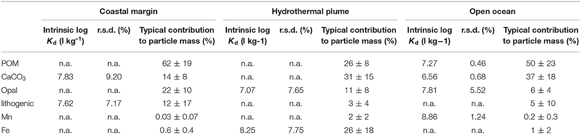
Table 4. The log intrinsic $K_{\text{d}}^{\text{i}}$ (l kg⁻¹) of Hg for six particle composition in the small size fraction (SSF) in coastal margin, hydrothermal plume, and open ocean of the Pacific, respectively, and their relative standard deviation (r.s.d.) as well as particle composition mass contribution (f; %).

The Lack of a Resolved Intrinsic K_d for Opal

Zaferani et al. have recently documented uncommonly high sediment accumulation fluxes of Hg that are also associated with high opal fluxes along parts of the Antarctic margin (e.g., Zaferani et al., 2018; Zaferani and Biester, 2020). This is seemingly inconsistent with our finding that there is little correlation between the values of bulk K_d and f_opal in overall datasets, resulting in undefined values for the intrinsic K_d for Hg-opal, and implying either that biogenic silica is a poor sorbent material for Hg or that diatoms are not particularly effective at taking up Hg. The first of these two possibilities are more likely as the high Hg fluxes on the Antarctic margin could be due more to high productivity, and therefore high abundance of particulate organic matter, rather than the opal associated with that productivity. Furthermore, diatoms appear to effectively bioaccumulate Hg (Mason et al., 1996; Bełdowska et al., 2018). The lack of a resolved K_d contribution from opal in the multivariate linear regression is an expression of an apparent lack of co-variation between K_d and f_opal and is consistent with both the simple correlation matrix view of the data as well as the PCA, both of which show little co-variation of Hg K_d and f_opal in the full datasets. One important caveat to this discussion is that two of the Pacific sub-datasets (open ocean and hydrothermal plume; Table 4), did have resolved intrinsic K_d's for opal, and the values were quite high. This was especially surprising as these were locations in the Pacific with the lowest fraction of particle mass as opal. With our current datasets, this behavior is difficult to explain and is worthy of further study.

Possible Biological Control on K_d in Surface Waters

In surface water, we found higher bulk K_d values in the open ocean compared to the continental margin (water depth < 200 m; Figure 3). This could be the result of the concentration effect as margin water tends to be higher in SPM than open ocean water. It could also be due to a difference in the mechanism by which Hg becomes associated with particles. In deeper waters, this should only be a consequence of sorption, while in surface waters could also be from biological uptake. If this is true, then variations in the value of bulk K_d might be determined by an “uptake efficiency.” In coastal regions, even though the biological activity is high, the uptake efficiency of Hg might be limited by the size of microbes based on Michaelis-Menten kinetics: more effective uptake occurs in the open ocean, where small size microbes with high uptake rate survive. In order to test this hypothesis, we examined the regression of log bulk K_d against log SPM in both shallow water (above 100 m) and deep water (below 100 m), separately, for three ocean basins. Then, we compared regression slopes between shallow and deep water by applying Z-test. Assuming that the particle concentration effect controls the K_d in deep water, if microbes were to passively adsorb Hg (like particle scavenging) in the surface, we would expect to see no difference between slopes in the shallow and deep water. In contrast, if microbes actively taking up Hg in the surface is responsible for the higher open ocean surface K_d, we might expect to observe a significantly different slope in shallow water compared to deep water, because K_d was not controlled by particle concentration effect.

The statistical results were summarized in Supplementary Table 3. Through the comparison of slopes of regression in shallow and deep seawater, we noticed that the slopes between shallow and deep water were not significantly different in the Atlantic and Arctic Ocean, suggesting the passive adsorption might take over in the surface seawater, therefore, we can deem that particle scavenging dominate the whole Atlantic and Arctic Ocean. However, the slope analysis failed the Z-test in the Pacific, the result of statistical difference between shallow and deep water is consistent with our hypothesis of active biological uptake control in the surface. Despite this observed difference, more evidence needs to be collected in order to support the phenomenon in the Pacific, we cannot assert the conclusion of surface domination of biological uptake on K_d, since the special feature in Hydrothermal Plume could also give rise to this difference between shallow and deep water.

Model Evaluation: Observed vs. Predicted

To test the robustness of the six end-member model, we substituted calculated values from Table 1 (intrinsic K_d) into Equation 2 to obtain the predicted K_d values for each sample (Tang et al., 2017). We then looked at the correlation between observed and predicted K_d through linear regressions and treating the ocean basins separately. The analysis of the coefficient of determination (R²) revealed that 12% of total variance was explained by the predicted vs. observed K_d regression model in Pacific (without hydrothermal plume data), while 14% of Atlantic K_d and 27% of Arctic K_d were explained by the linear regression of predicted against observed K_d (PO regression), respectively (P < 0.0001).

Furthermore, all the slopes were far from 1, the shape of linear regression in Figure 8 suggested that this model overestimates observed K_d at low value while underestimates at high value. The y-intercepts from PO regression were different from 0. Therefore, based on the analysis of R², slope and y-intercept, this model failed to describe the characteristic of variability of observed K_d well. However, when we re-did the linear regression on extracted data from hydrothermal vents in the Pacific only (Figure 8D), the slope was 0.89 with R² 0.84. This good agreement occurred because iron oxyhydroxides were a significant fraction of particle mass (26%) and thus dominated the adsorption (97%) in the whole hydrothermal plume area (Figures 7G,H). This evaluation is informative, suggesting we need to look for a new way to express the partition coefficient in the future.

FIGURE 8

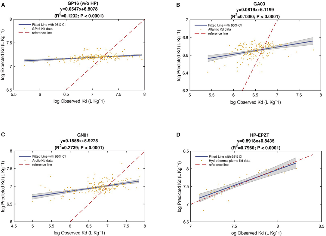
Figure 8. The statistical results of the regression of observed (Obs) vs. predicted (Pre) K_d values in (A) the Pacific Ocean (GP16) without Hydrothermal Plume (HP), (B) the Atlantic Ocean (GA03), (C) the Arctic Ocean (GN01), and (D) Hydrothermal plume in the EPZT. Bule solid line is linear regression fitted line, red dash line is a reference line y = x.

Implication of Hg Residence Time

To some extent, the K_d determines the downward Hg flux from the surface ocean, and further influences the Hg burial flux to marine sediments, which give us insights into the residence time of Hg in the ocean.

Here, we calculated the Hg inventory in each ocean basin by integrating the dissolved Hg with depth (Table 5). Due to a lack of Hg burial flux on a global scale, we used information about the particulate Hg flux into the deep ocean to estimate the burial flux. The particulate Hg flux was derived based on the bulk particle flux from the same cruises (Xiang et al., 2020). To convert to Hg flux, we multiplied the particle flux by the concentration ratios between particulate Hg and SPM for each sample. The underlying assumptions are: (1) particulate Hg follows the particle size distribution of bulk particles; (2) particulate Hg has the same sinking velocity as bulk particles. We then estimated the mean of the logarithmic transformed Hg sinking fluxes below 3,500 m in each ocean basin, and assumed the average sinking flux in the deep ocean equal to burial flux. Overall, our estimates of the Hg burial flux were an order of magnitude higher in the Pacific than the Arctic and Atlantic Ocean (Table 5). In the Arctic Ocean, the Hg burial flux (20.23, +10.26, −6.81 pmole m⁻² d⁻¹) was in a similar range compared to Tesán Onrubia et al. (2020) (outer shelf: 51 ± 35 pmole m⁻² d⁻¹; central Arctic Ocean: 11 ± 8 pmole m⁻² d⁻¹). Note that the uncertainty of burial flux were not the same because they were transformed back from logarithmic to their original scale. Additionally, the Hg burial fluxes in the Atlantic and Arctic were in line with the globally averaged Hg fluxed from deep ocean to sediments reported by Outridge et al. (2018), which was 0.60 kt/y.

TABLE 5

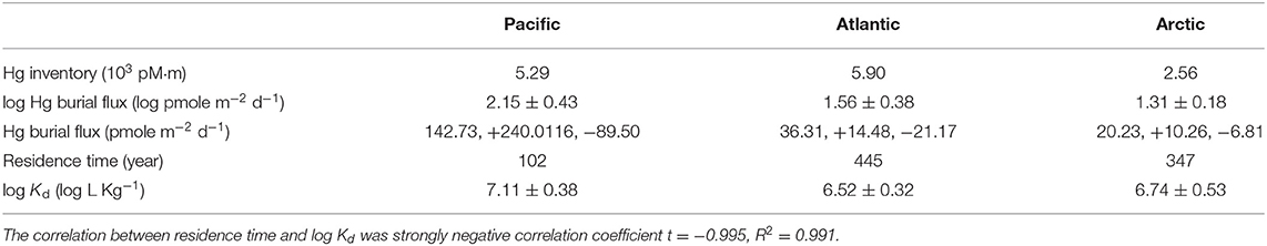
Table 5. Summary of estimated Hg inventory (10³ pM·m), Hg burial flux (pmole m⁻² d⁻¹) with asymmetric standard deviation, Hg residence time (year), as well as averaged log K_d (log L Kg⁻¹) in the Pacific, Atlantic, and Arctic Ocean, respectively.

On the basis of estimated Hg inventory and burial fluxes, Hg residence times in three ocean basins were calculated (Table 5). A strong negative correlation between log bulk K_d and residence time was observed in our analysis, suggesting that K_d could have a significant impact on Hg residence time. Given the higher bulk K_d observed in the Pacific, our estimates of the Hg residence time in the Pacific are the shortest among all oceans, ~102 years, lower than previous studies (~350 yrs, e.g., Gill and Fitzgerald, 1988). The residence time of Hg is the longest in the Atlantic. It should be noted that, however, our Stokes' law-based method might overestimate the Hg burial fluxes compared to conventional but limited sediment trap-based observations (e.g., Munson et al., 2015), which could lead to shorter residence time. Future modeling and field observation efforts are needed to better constrain the Hg burial flux and thereby Hg residence time on a global scale.

Conclusion

In general, we investigated into the Hg partition coefficient (K_d) in the water column across the Pacific, Atlantic and Arctic Ocean, and analyzed the impact of particle concentration and composition on variation of K_d. The higher K_d were observed in the Pacific, while modestly lower and lowest K_d were observed in the Arctic and Atlantic Ocean, respectively. The log bulk K_d of Hg was inversely correlated with log SPM concentration, known as “particle concentration effect.” The analysis of intrinsic K_d across three ocean basins indicated that affinity of Hg to particle composition is not constant everywhere, and its variation depends on regions and phase concentration. Fe and Mn oxides have highly strong affinity to Hg in the water column despite their low relative abundance in particles, which could be dominant phases in some special regions like the hydrothermal plume, POM and CaCO₃ were important drivers of K_d as well. Further, the end member mixing model has limited ability to describe the observed K_d for the entire ocean possibly as a result of changing water chemistry and mineralogy of particles. Overall, the SPM combined particle composition explained the 28–66% of variance of K_d over three ocean basins. The strong negative correlation between Hg residence time and average log bulk K_d implied that varying K_d might determine the timescale of marine Hg cycling indirectly.

Data Availability Statement

Publicly available datasets were analyzed in this study. This data can be found at: https://www.bco-dmo.org.

Author Contributions

XC and CL conceived of the presented idea and took the lead in writing the manuscript. XC performed the computations and analytical calculation. PL and YX collected the SPM datasets. CH and CL collected Hg datasets. All authors provided critical feedback and contributed to the final manuscript.

Funding

XC was supported during the analysis and writing of this current work by the Chinese Scholarship Council. Original support for collection and analysis of these samples came from the U.S. National Science Foundation in grants to CL and CH (OCE 1534315; OCE 1434653; OCE 1132515; OCE 1232760; OCE 0928191).

Conflict of Interest

The authors declare that the research was conducted in the absence of any commercial or financial relationships that could be construed as a potential conflict of interest.

Acknowledgments

We thank the captains and crews of GEOTRACES cruises GN01, GA03, and GP16, as well as the scientific crews who collected the samples. The underlying data are archived at BCO-DMO (https://www.bco-dmo.org.) and we thank their on-going efforts regarding data quality and access. We also thank the US and International GEOTRACES offices for pre-COVID travel support and publicity. We thank Claudie Beaulieu for advice with PCA.

Supplementary Material

The Supplementary Material for this article can be found online at: https://www.frontiersin.org/articles/10.3389/fenvc.2021.660267/full#supplementary-material

References

Agather, A. M., Bowman, K. L., Lamborg, C. H., and Hammerschmidt, C. R. (2019). Distribution of mercury species in the Western Arctic ocean (US GEOTRACES GN01). Mar. Chem. 216:103686. doi: 10.1016/j.marchem.2019.103686

CrossRef Full Text | Google Scholar

Amos, H. M., Jacob, D. J., Streets, D. G., and Sunderland, E. M. (2013). Legacy impacts of all-time anthropogenic emissions on the global mercury cycle. Glob. Biogeochem. Cycles 410–421. doi: 10.1002/gbc.20040

CrossRef Full Text | Google Scholar

Anderson, R. F. (2014). “8.9 - Chemical tracers of particle transport,” in Treatise on Geochemistry (Second Edition), eds. H. D. Holland and K. K. Turekian (Oxford: Elsevier), 259–280. doi: 10.1016/B978-0-08-095975-7.00609-4

CrossRef Full Text | Google Scholar

Bacon, M., Spencer, D., and Brewer, P. (1976). 210Pb/226Ra and 210Po/210Pb disequilibria in seawater and suspended particulate matter. Earth Planet. Sci. Lett. 32, 277–296. doi: 10.1016/0012-821X(76)90068-6

CrossRef Full Text | Google Scholar

Bacon, M. P., and Anderson, R. F. (1982). Distribution of thorium isotopes between dissolved and particulate forms in the deep sea. J. Geophys. Res. 87, 2045–2056. doi: 10.1029/JC087iC03p02045

CrossRef Full Text | Google Scholar

Balcom, P. H., Hammerschmidt, C. R., Fitzgerald, W. F., Lamborg, C. H., and O'connor, J. S. (2008). Seasonal distributions and cycling of mercury and methylmercury in the waters of New York/New Jersey harbor estuary. Mar. Chem. 109, 1–17. doi: 10.1016/j.marchem.2007.09.005

CrossRef Full Text | Google Scholar

Bam, W., Maiti, K., Baskaran, M., Krupp, K., Lam, P. J., and Xiang, Y. (2020). Variability in 210Pb and 210Po partition coefficients (Kd) along the US GEOTRACES Arctic transect. Mar. Chem. 219:103749. doi: 10.1016/j.marchem.2020.103749

CrossRef Full Text | Google Scholar

Baskaran, M., and Santschi, P. H. (1993). The role of particles and colloids in the transport of radionuclides in coastal environments of Texas. Mar. Chem. 43, 95–114. doi: 10.1016/0304-4203(93)90218-D

CrossRef Full Text | Google Scholar

Bełdowska, M., Zgrundo, A., and Kobos, J. (2018). Mercury in the diatoms of various ecological formations. Water Air Soil Pollut. 229:168. doi: 10.1007/s11270-018-3814-1

PubMed Abstract | CrossRef Full Text | Google Scholar

Benoit, G., and Rozan, T. F. (1999). The influence of size distribution on the particle concentration effect and trace metal partitioning in rivers. Geochim. Cosmochim. Acta 63, 113–127. doi: 10.1016/S0016-7037(98)00276-2

CrossRef Full Text | Google Scholar

Biscaye, P. E. (1965). Mineralogy and sedimentation of recent deep-sea clay in the atlantic ocean and adjacent seas and oceans. GSA Bull. 76, 803–832. doi: 10.1130/0016-7606(1965)76[803:MASORD]2.0.CO;2

CrossRef Full Text | Google Scholar

Bowman, K. L., Hammerschmidt, C. R., Lamborg, C. H., and Swarr, G. (2015). Mercury in the North Atlantic ocean: the U.S. GEOTRACES zonal and meridional sections. Deep Sea Res. Part II Top. Stud. Oceanogr. 116, 251–261. doi: 10.1016/j.dsr2.2014.07.004

CrossRef Full Text | Google Scholar

Bowman, K. L., Hammerschmidt, C. R., Lamborg, C. H., Swarr, G. J., and Agather, A. M. (2016). Distribution of mercury species across a zonal section of the eastern tropical South Pacific ocean (U.S. GEOTRACES GP16). Mar. Chem. 186, 156-166. doi: 10.1016/j.marchem.2016.09.005

CrossRef Full Text | Google Scholar

Cael, B., and White, A. E. (2020). Sinking versus suspended particle size distributions in the North Pacific subtropical gyre. Geophys. Res. Lett. 47:e2020GL087825. doi: 10.1029/2020GL087825

CrossRef Full Text | Google Scholar

Chase, Z., Anderson, R. F., Fleisher, M. Q., and Kubik, P. W. (2002). The influence of particle composition and particle flux on scavenging of Th, Pa and Be in the ocean. Earth Planet. Sci. Lett. 204, 215–229. doi: 10.1016/S0012-821X(02)00984-6

CrossRef Full Text | Google Scholar

Darby, D. A. (1975). Kaolinite and other clay minerals in Arctic ocean sediments. J. Sediment. Res. 45, 272–279. doi: 10.1306/212F6D34-2B24-11D7-8648000102C1865D

CrossRef Full Text | Google Scholar

Efron, B., and Stein, C. (1981). The jackknife estimate of variance. Ann. Stat. 9, 586–596. doi: 10.1214/aos/1176345462

CrossRef Full Text | Google Scholar

Fitzgerald, W. F., Engstrom, D. R., Lamborg, C. H., Tseng, C.-M., Balcom, P. H., and Hammerschmidt, C. R. (2005). Modern and historic atmospheric mercury fluxes in northern Alaska: global sources and arctic depletion. Environ. Sci. Technol. 39, 557–568. doi: 10.1021/es049128x

PubMed Abstract | CrossRef Full Text | Google Scholar

Fitzgerald, W. F., and Lamborg, C. H. (2014). “Geochemistry of mercury in the environment,” in Treatise on Geochemistry, ed. B. S. Lollar (Oxford: Elsevier), 91–129. doi: 10.1016/B978-0-08-095975-7.00904-9

CrossRef Full Text | Google Scholar

Gill, G. A., and Fitzgerald, W. F. (1988). Vertical mercury distributions in the oceans. Geochim. Cosmochim. Acta 52, 1719–1728. doi: 10.1016/0016-7037(88)90240-2

CrossRef Full Text | Google Scholar

Hammerschmidt, C. R., and Fitzgerald, W. F. (2004). Geochemical controls on the production and distribution of methylmercury in near-shore marine sediments. Environ. Sci. Technol. 38, 1487–1495. doi: 10.1021/es034528q

PubMed Abstract | CrossRef Full Text | Google Scholar

Hayes, C. T., Anderson, R. F., Fleisher, M. Q., Vivancos, S. M., Lam, P. J., Ohnemus, D. C., et al. (2015). Intensity of Th and Pa scavenging partitioned by particle chemistry in the North Atlantic ocean. Marine Chem. 170, 49–60. doi: 10.1016/j.marchem.2015.01.006

CrossRef Full Text | Google Scholar

Honeyman, B. D., Balistrieri, L. S., and Murray, J. W. (1988). Oceanic trace metal scavenging: the importance of particle concentration. Deep Sea Res. Part A Oceanogr. Res. Pap. 35, 227–246. doi: 10.1016/0198-0149(88)90038-6

CrossRef Full Text | Google Scholar

Honeyman, B. D., and Santschi, P. H. (1989). A brownian-pumping model for oceanic trace-metal scavenging - evidence from Th-isotopes. J. Marine Res. 47, 951–992. doi: 10.1357/002224089785076091

CrossRef Full Text | Google Scholar

John, S. G., and Conway, T. M. (2014). A role for scavenging in the marine biogeochemical cycling of zinc and zinc isotopes. Earth Planet. Sci Lett. 394, 159–167. doi: 10.1016/j.epsl.2014.02.053

CrossRef Full Text | Google Scholar

Lam, P. J., Lee, J.-M., Heller, M. I., Mehic, S., Xiang, Y., and Bates, N. R. (2018). Size-fractionated distributions of suspended particle concentration and major phase composition from the U.S. GEOTRACES eastern Pacific zonal transect (GP16). Marine Chem. 201, 90–107. doi: 10.1016/j.marchem.2017.08.013

CrossRef Full Text | Google Scholar

Lam, P. J., Ohnemus, D. C., and Auro, M. E. (2015). Size-fractionated major particle composition and concentrations from the US GEOTRACES North Atlantic zonal transect. Deep Sea Res. Part II Top. Stud. Oceanogr. 116, 303–320. doi: 10.1016/j.dsr2.2014.11.020

CrossRef Full Text | Google Scholar

Lamborg, C. H., Hammerschmidt, C. R., and Bowman, K. L. (2016). An examination of the role of particles in oceanic mercury cycling. Philos. Trans. A Math. Phys. Eng. Sci. 374:20150297. doi: 10.1098/rsta.2015.0297

PubMed Abstract | CrossRef Full Text | Google Scholar

Lerner, P., Marchal, O., Lam, P. J., Buesseler, K., and Charette, M. (2017). Kinetics of thorium and particle cycling along the US GEOTRACES north Atlantic transect. Deep Sea Res. Part I Oceanogr. Res. Pap. 125, 106–128. doi: 10.1016/j.dsr.2017.05.003

CrossRef Full Text | Google Scholar

Lerner, P., Marchal, O., Lam, P. J., and Solow, A. (2018). Effects of particle composition on thorium scavenging in the north Atlantic. Geochim. Cosmochim. Acta 233, 115–134. doi: 10.1016/j.gca.2018.04.035

CrossRef Full Text | Google Scholar

Mason, R. P., Reinfelder, J. R., and Morel, F. M. (1996). Uptake, toxicity, and trophic transfer of mercury in a coastal diatom. Environ. Sci. Technol. 30, 1835–1845. doi: 10.1021/es950373d

CrossRef Full Text | Google Scholar

Moran, S., Yeats, P., and Balls, P. (1996). On the role of colloids in trace metal solid-solution partitioning in continental shelf waters: a comparison of model results and field data. Cont. Shelf Res. 16, 397–408. doi: 10.1016/0278-4343(95)98840-7

CrossRef Full Text | Google Scholar

Munson, K. M., Lamborg, C. H., Swarr, G. J., and Saito, M. A. (2015). Mercury species concentrations and fluxes in the central tropical Pacific ocean. Glob. Biogeochem. Cycles 29, 656–676. doi: 10.1002/2015GB005120

CrossRef Full Text | Google Scholar

Outridge, P. M., Mason, R. P., Wang, F., Guerrero, S., and Heimbürger-Boavida, L. E. (2018). Updated global and oceanic mercury budgets for the united nations global mercury assessment 2018. Environ. Sci. Technol. 52, 11466–11477. doi: 10.1021/acs.est.8b01246

PubMed Abstract | CrossRef Full Text | Google Scholar

Resing, J. A., Sedwick, P. N., German, C. R., Jenkins, W. J., Moffett, J. W., Sohst, B. M., et al. (2015). Basin-scale transport of hydrothermal dissolved metals across the South Pacific Ocean. Nature 523, 200–203. doi: 10.1038/nature14577

PubMed Abstract | CrossRef Full Text | Google Scholar

Soerensen, A. L., Jacob, D. J., Schartup, A. T., Fisher, J. A., Lehnherr, I., St. Louis, V. L., et al. (2016). A mass budget for mercury and methylmercury in the Arctic ocean. Global Biogeochem. Cycles 30, 560–575. doi: 10.1002/2015GB005280

CrossRef Full Text | Google Scholar

Stemmann, L., and Boss, E. (2012). Plankton and particle size and packaging: from determining optical properties to driving the biological pump. Ann. Rev. Mar. Sci. 4, 263–290. doi: 10.1146/annurev-marine-120710-100853

PubMed Abstract | CrossRef Full Text | Google Scholar

Tang, Y., Stewart, G., Lam, P. J., Rigaud, S., and Church, T. (2017). The influence of particle concentration and composition on the fractionation of Po-210 and Pb-210 along the north Atlantic GEOTRACES transect GA03. Deep Sea Res. Part I Oceanogr. Res. Pap. 128, 42–54. doi: 10.1016/j.dsr.2017.09.001

CrossRef Full Text | Google Scholar

Tesán Onrubia, J. A., Petrova, M. V., Puigcorbé, V., Black, E. E., Valk, O., Dufour, A., et al. (2020). Mercury export flux in the Arctic ocean estimated from 234Th/238U disequilibria. ACS Earth Space Chem. 4, 795–801. doi: 10.1021/acsearthspacechem.0c00055

CrossRef Full Text | Google Scholar

Xiang, Y., and Lam, P. J. (2018). “Comparisons of size-fractioned suspended particles in three different basins from the US GEOTRACES NAZT (GA03), EPZT (GP16) and Arctic (GN01) Cruises,” in 2018 Ocean Sciences Meeting (Portland, OR: AGU).

Google Scholar

Xiang, Y., and Lam, P. J. (2020). Size-Fractionated compositions of marine suspended particles in the western Arctic ocean: lateral and vertical sources. J. Geophys. Res. Oceans 125:e2020JC016144. doi: 10.1029/2020JC016144

CrossRef Full Text | Google Scholar

Xiang, Y., Lam, P. J., and Burd, A. B. (2020). Controls on Sinking Velocities and Mass Fluxes of Size-Fractionated Marine Particles in Recent U.S. GEOTRACES Cruises. Available online at: https://essoar.org.

Zaferani, S., and Biester, H. (2020). Biogeochemical processes accounting for the natural mercury variations in the southern ocean diatom ooze sediments. Ocean Sci. Discuss. 2020, 1–22. doi: 10.5194/os-16-729-2020

CrossRef Full Text | Google Scholar

Zaferani, S., Pérez-Rodríguez, M., and Biester, H. (2018). Diatom ooze—a large marine mercury sink. Science 361, 797–800. doi: 10.1126/science.aat2735

PubMed Abstract | CrossRef Full Text | Google Scholar

Zhang, Y., Jaeglé, L., and Thompson, L. (2014). Natural biogeochemical cycle of mercury in a global three-dimensional ocean tracer model. Global Biogeochem. Cycles 28, 2014GB004814. doi: 10.1002/2014GB004814

CrossRef Full Text | Google Scholar