Accelerations of public transport vehicles: A method to derive representative generic pulses for passenger safety testing

Introduction

Public buses and trams are not only environmentally friendly and affordable but are also a safe means of transportation compared to other modes of urban transport such as private cars, powered two-wheelers and bicycles (Morency et al., 2018; European Commission, 2022). Nevertheless, using public transportation to travel is not without risk. Most injuries that passengers sustain while using public transportation occur without the vehicle being involved in a road collision (Kirk et al., 2003) (so-called non-collision incidents). Particularly standing passengers can lose their balance and fall due to the acceleration and deceleration behaviour of the vehicle; Elvik (2019) estimated the risk of falling in a moving public transport vehicle as 0.3–0.5 per million passenger kilometres and 0.7–1.7 per million passengers in relation to boarding and exiting the vehicle. The injury risk is higher for female and elderly passengers (Halpern et al., 2005; Kendrick et al., 2015; Li et al., 2017). In addition to these safety concerns, passenger dissatisfaction with the comfort and smoothness of the ride is also one of the major reasons to avoid bus service (Karekla and Tyler, 2018).

To understand the typical injury mechanisms in non-collision incidents, both the postural balance of a person standing on a moving surface and the nature of the acceleration perturbations typically challenging the balance of a bus or tram passenger have been studied. While the postural balance of a person standing on a moving surface is not directly the subject of this study, the work in this field using either laboratory experiments with voluntary participants (e.g., (Carpenter et al., 2005; Robert et al., 2007; Tokuno et al., 2010)) or computational models that simulate the human body (Palacio et al., 2009; Aftab et al., 2016) is still a primary research motivation. The acceleration signal of a typical public transport journey is of a duration that by far exceeds the range of motion of a laboratory sled experiment and the duration that can be replicated in a human body model simulation within reasonable computation time. Therefore, the characteristic features of the acceleration perturbations must be 1) understood and 2) condensed into short pulses that can be applied in a computer simulation or in the laboratory.

In early research on the acceleration behaviour of public transport vehicles, the focus was mostly on defining comfort or safety thresholds for acceleration magnitudes and jerks (Hoberock, 1977; Brooks et al., 1978), while the structure of the acceleration pulses was not investigated in further detail. The first study that considered the influence of acceleration pulses on the postural balance of standing passengers was completed by Graaf and Van Weperen (1997), who measured acceleration time series on buses and trams and used similar perturbations in treadmill experiments with volunteer participants. More recently, several authors studied the acceleration time series of buses (Zaworski et al., 2007) and subway trains (Powell and Palacín, 2015) with a focus on passenger (dis)comfort. The shape of average emergency braking pulses was investigated by Turkovich et al. (2011); Schubert et al. (2017) measured acceleration pulses during a study with a bus in test driving conditions using volunteers. However, a closer analysis of the acceleration time series was not the main objective of their work. To date, the most systematic study investigating the structure and shape of acceleration pulses was completed by Kirchner et al. (2014). These authors expanded time-normalised acceleration and deceleration pulses in a Legendre series, enabling the quantification of the relevant properties of the pulses and the comparison of different acceleration events in terms of similarity coefficients. They also suggested a method to choose a representative example out of a given set of pulses (i.e., the one with the highest mean mutual similarity).

Despite the research completed thus far, with a goal of providing suitable input data for computational and laboratory studies of the standing passenger problem, there are still significant gaps in both knowledge and methodology. Representative sets of field data are still rare in the current literature. In addition, there is no method to automatically derive meaningful average acceleration and deceleration pulses from larger data sets. Even though the method presented by Kirchner et al. (2014) already allows for a systematic comparison of different acceleration and deceleration events, their method is not readily applicable to larger datasets, as it requires manual splitting of the acceleration signals. Furthermore, an averaging method taking into account all events of a set (instead of only choosing a representative example) is still lacking in the literature.

In this work, we address this methodological gap by expanding the (Kirchner et al., 2014) method to an automatically applicable algorithm that can be used for datasets of much larger sizes. Furthermore, we propose a weighted-mean method to compute an average pulse from a given set of acceleration and deceleration pulses. As a demonstration of the method, we present a set of real-life acceleration data recorded on public buses during their normal operation in city traffic, from which we derive generic acceleration and deceleration pulses representing the typical behaviour of the vehicles under consideration.

Even though a combination of theoretical work and field data analysis, this article still follows the structure ”Materials and methods—Results—Discussion—Conclusion” typical for a data analysis work. The section ”Materials and methods” contains a somewhat longer theoretical section, explaining the proposed data analysis method, including some theoretical background on Legendre expansions and a description of the new ”weighted mean” approach and the splitting algorithm. The remaining parts focus on the application of the new method to the dataset. For the reader interested in the deeper mathematical details of the weighted mean approach, more information is provided in the appendix.

Materials and methods

Data analysis method

The time series analysis method presented here is based on a Legendre expansion of a scalar function with support [0, 1], which represents a time-normalised acceleration or deceleration event. Therefore, the raw datasets (i.e., the time series of the longitudinal acceleration component) first have to be filtered and split into acceleration and deceleration events. Then, normalisation and Legendre expansion of the data is completed. The resulting coefficient sets can be used for similarity analysis and the computation of representative average pulses. The implementation of the data analysis method was achieved in Python using the SciPy and Pandas packages (McKinney, 2010; Virtanen et al., 2020). All scripts are available under the terms of the GPL licence on the OpenVT platform.¹

Preprocessing and automatic splitting

The one-dimensional raw acceleration data are Butterworth filtered (second order, cutoff frequency ${\omega }_0=0.75\frac{\text{rad}}{\text{s}}$) to remove high-frequency oscillations. The resulting acceleration signal is split according to the following three-step algorithm:

• Constant phases are identified as intervals that are longer than a certain duration, which by default is 100 time steps, and the change of the signal per time step is lower than a certain threshold, which by default is 0.005 standard deviations of the entire signal. After cropping out these constant phases, a set of raw pulses remains.

• On each of the remaining raw pulses, a discrete Fourier transformation is applied and the maximum of the spectrum is determined. If the peak occurs at a frequency $>0$, i.e., there is predominant oscillating behaviour, then the pulse is split into multiples of the period associated with the peak frequency, and if the spectral maximum occurs at 0, i.e., there is no predominant oscillating behaviour, then the peak is not split.

• For each of the resulting subpulses, the cumulative sum is calculated (as an approximate estimate of the resulting speeds) and the absolute maximum of the result is determined. Depending on whether the maximum occurs 1) close to the start of the subpulse, 2) close to the end of the subpulse, or 3) somewhere in between subpulses, the subpulse is identified as 1) a deceleration event (DEC), 2) an acceleration event (ACC) or 3) a split at the occurrence of the maximum of an ACC and a DEC event².

As a result of the splitting algorithm, for the given time series, two sets of functions representing the acceleration signals of the ACC and the DEC events, respectively, are obtained. For further treatment, these functions are time-normalised to a unity interval, resulting in the functions

$f_i^I:\left[\mathrm{0,1}\right]\mapsto \mathbb{R},(1)$

where 1 ≤ i ≤ M_I is the number of the event in the given set and I ∈ {A₁, A₂, …, , D₁, D₂, …} is an identifier representing the different sets of ACC pulses (A_n) and DEC pulses (D_m), respectively. That is, if only one acceleration time series is considered, the algorithm results in one set of ACC pulses and one of DEC pulses, so the identifier could be I ∈ {A₁, D₁}, while for each additional time series under consideration, one more ACC and DEC set is added to the list.³

Legendre expansion

Expansions in Legendre polynomials are a known and useful tool, e.g., in image processing (Paton, 1975). The mathematical properties of these expansions and their convergence are well documented in the scientific literature. For an overview, see Wang and Xiang (2012). Kirchner et al. (2014) suggested a Legendre expansion of acceleration pulses due to the convenient properties of the Legendre polynomials on a unit interval.

As opposed to the most common representation on the interval [−1, 1], in this work, the shifted Legendre polynomials on the support [0, 1] are used. For any non-negative integer n, the nth polynomial is defined as

$P_n:\left[\mathrm{0,1}\right]\mapsto \mathbb{R},(2)$

$P_n\left(x\right)=\frac{1}{n!}\frac{{\text{d}}^n}{\text{d}{x}^n}{\left(x^2-x\right)}^n.(3)$

These polynomials obey the orthogonality relation

${\int }_0^1{P}_k\left(x\right)P_l\left(x\right)\text{d}x=\frac{1}{2k+1}{\delta }_{kl},(4)$

on which the Legendre expansion is based.

The time-normalised functions in Eq. 1 can be approximated by a series of Legendre polynomials,

$f_i^I\left(x\right)=\sum _{k=0}^N{c}_{i,k}^I{P}_k\left(x\right)+{\left(R_N\right)}_i^I\left(x\right)\approx \sum _{k=0}^N{c}_{i,k}^I{P}_k\left(x\right),(5)$

where N is the order of the approximation and ${\left(R_N\right)}_i^I(x)$ are the residual functions. The decay of the residuals with N depends on the behaviour of the complex continuation of the function f on a Bernstein ellipse. In general, this decay cannot easily be estimated. For further details see, e.g., Wang and Xiang (2012). However, for our purposes, it can be stated that choices on an order of magnitude of N = 10 to N = 200 are reasonable, in a trade-off of approximation quality and computational cost.

Using the orthogonality relation Eq. 4, the N + 1 Legendre coefficients can be written as

$c_{i,k}^I=\left(2k+1\right){\int }_0^1{f}_i^I\left(x\right)P_k\left(x\right)\text{d}x.(6)$

Please note that, for the sake of the clarity, we will in the following often use a somewhat sloppy notation and denote the coefficient $c_{i,k}^I$ by c_i,k provided that it is clear from which set I the corresponding pulse $f_i^I$ is taken.

Our implementation offers two ways to compute the Legendre coefficients: 1) a numerical evaluation of the integrals in Eq. 6 using a Gauss-Legendre quadrature with the roots of the highest-order polynomial as integration points (to which the data are interpolated using a cubic spline interpolation) and 2) a least-squares fit of the data with Eq. 5 (this method avoids evaluating the integrals explicitly). Method (ii) tends to be faster, and method (i) is more stable for coefficients of higher order⁴.

The Legendre approximation reduces the number of degrees of freedom for each pulse to a small number of coefficients; the use of 40–70 coefficients is mostly sufficient, except if jerks are to be estimated. In addition, this approximation provides a straightforward way to compare the shapes of different pulses (see section “Similarity analysis”).

Analysis of time-normalised acceleration and deceleration pulses

Once the Legendre representations (5) have been computed, several methods can be employed to compare the different pulses.

Jerk estimation

The jerk, i.e., the time derivative of acceleration, is known to be of fundamental importance for passenger (dis)comfort and safety (Graaf and Van Weperen, 1997). Nevertheless, this quantity (and particularly its peak value) is not necessarily easy to estimate from acceleration time series, as numerical differentiation schemes tend to be unstable for noisy data.

Once the Legendre coefficients of a given pulse are known, we compute the Legendre representation of the time derivative according to Phillips (1988). The corresponding Legendre expansion provides up to a scaling factor due to the time normalisation, an approximation of the jerk as a function of normalised time. This method avoids using a finite differences scheme⁵. However, this method requires the computation of a higher number of Legendre coefficients.

For the jerk as time derivative of acceleration, is has to be taken into account whether or not the acceleration pulses under consideration are time-normalised. The jerk estimation method for time-normalised pulses described above yields a jerk with respect to normalised time, with a dimension of acceleration. If the “true” jerk (dimension acceleration over time) is of interest, the jerk with respect to normalised time has to be divided by the duration of the pulse under consideration. In the results section, the histograms for the measured pulses always show the jerk with respect to time, while the jerks of the mean and maximum similarity pulses are specified with respect to normalised time.

Similarity analysis

The similarity analysis in terms of Legendre coefficients has been described by Kirchner et al. (2014). For two time-normalised ACC or DEC pulses f and g, the similarity coefficient is defined as

$s\left[f,g\right]=\frac{⟨f,g⟩}{\sqrt{⟨f,f⟩⟨g,g⟩}},(7)$

where $⟨.,.⟩$ represents the L2 scalar product. Similarity coefficients can be applied to compare time-normalised pulses of different sets without taking into account their magnitudes. We will, however, in the following focus on similarities between pulses of the same set.

Let $\left\{f_1^I\dots f_M^I\right\}$ be a set of M time-normalised pulses (all either ACC or DEC pulses) with identifier I (in the following, only this one set of pulses will be considered, so we will drop the identifier I in the notation). Using a Legendre expansion to order N, the similarity coefficient within the set can be expressed in terms of the Legendre coefficients c_i,k, c_j,k of the pulses f_i and f_j as

$s_{ij}≔s\left[f_i,f_j\right]=\frac{{\sum }_{k=0}^N\frac{c_{i,k}{c}_{j,k}}{2k+1}}{\sqrt{{\sum }_{l=0}^N\frac{{\left(c_{i,l}\right)}^2}{2l+1}{\sum }_{m=0}^N\frac{{\left(c_{j,m}\right)}^2}{2m+1}}}.(8)$

For the M different pulses f_i of the set under consideration, a symmetric similarity matrix of dimensions M × M containing the M(M + 1)/2 independent similarity coefficients is obtained.

Average/representative example: Maximum similarity and mean pulses

The similarity coefficients s_ij within a given set are the basis for different methods to define a representative average or to select a representative example for the shape characteristics of a set of time-normalised events without over-representing high-magnitude events. Kirchner et al. (2014) suggested considering the mean similarity coefficient of each pulse f_i out of the set I, which is defined as

${\bar{s}}_i=\frac{1}{M}\sum _{j=0}^M{s}_{ij}.(9)$

As a representative example, the pulse out of the set with the highest mean similarity coefficient is chosen,⁶

$f_{\text{maxsim}}^I=f_i\in \left\{f_1^I\dots f_M^I\right\}:{\bar{s}}_i={\max }_{k\in \left\{1\dots M\right\}}{\bar{s}}_k.(10)$

This pulse can now either be written as time-normalised function or as Legendre expansion. We will refer to this method as the “maximum similarity pulse method” and to the resulting pulse f_i as the “maximum similarity pulse”.

While the maximum similarity pulse method allows choosing a representative example out of a set of pulses, in many applications (particularly when creating input to experimental or numerical tests), it is more appropriate to use an average that takes into account the shape of all pulses of the set to some extent. Given that measured acceleration signals are typically sets with different magnitudes but similar shapes, simply calculating an arithmetic mean would not be very useful, as it would be dominated by pulses with the highest magnitude.

As a method to calculate such a representative average of the shapes of different pulses, we suggest considering a weighted mean over a given set with the inverse of the L₂-norm of each pulse as weight. The Legendre coefficients of this weighted mean pulse can be written as⁷

${\bar{c}}_k=a_0\frac{1}{M}\sum _{i=1}^M\frac{c_{i,k}}{\sqrt{{\sum }_{l=0}^N\frac{{\left(c_{i,l}\right)}^2}{2l+1}}},k=0\dots N,(11)$

where M, again, is the overall number of pulses in the given set, a₀ is an arbitrary (but constant) scaling factor, and N is the order of the Legendre approximation. The time-normalised acceleration pulse corresponding to these coefficients is given by the generic expression of the Legendre series (Eq. 5) with zero residuals, ${\sum }_{k=0}^N{\bar{c}}_k{P}_k(x)$. It can be shown (see appendix) that out of all Legendre series of order N, the multiples of this pulse have the highest possible mean similarity with the pulses of the set.⁸ As this holds for any multiple of the pulse define d by these coefficients, the maximisation of the mean similarity only defines the mean pulse up to a multiplicative factor. Therefore, Eq. 11 contains an unknown scaling factor a₀. The choice of the scaling factor is up to the user; a reasonable choice depends on the application. For example, the peak acceleration of the mean pulse could be adapted to the needs of a laboratory or numerical test, or it could be used to normalise either the L2-norm of the pulse or the peak acceleration to 1, so a time- and acceleration-normalised pulse would be obtained. In the examples given in the Results section, we choose a₀ as the arithmetic mean of the peak accelerations of the pulses of the input set, so a₀ contains some information about their magnitude. However, it shall be stressed that different choices of the normalisation are possible and can makes sense according to the desired application. In the following sections, the pulse defined by the coefficients in Eq. 11 will be referred to as the “mean pulse” (or “unconstrained mean pulse”) and the method as the “(unconstrained) mean pulse method.”

Due to the cutting algorithm and varying terrain gradients, measured acceleration pulses that are cut out of an acceleration time series tend to be offset or lopsided. Therefore, the mean pulses defined by the coefficients in Eq. 11 do not generally equal zero when x = 0 or x = 1. However, with a laboratory setting and computer simulations in mind, it is interesting to derive a version of the mean pulse that maximises the mean similarity with all pulses under consideration while starting and ending at zero. With the definitions

$\bar{c}=\sum _{k=0}^N{\bar{c}}_k,(12)$

$\tilde{c}=\sum _{k=0}^N{\bar{c}}_k{\left(-1\right)}^k,(13)$

we define the Legendre coefficients

${\bar{c}}_k^0={\bar{c}}_k-\frac{\left(2k+1\right)\left(N+1-{\left(-1\right)}^{N+k}\right)}{N\left(N+1\right)\left(N+2\right)}\left[\bar{c}+{\left(-1\right)}^k\tilde{c}\right],k=0,\dots ,N.(14)$

As for the “mean pulse” method, the corresponding time-normalised acceleration pulse can be computed according to Eq. 5, ${\sum }_{k=0}^N{\bar{c}}_k^0{P}_k(x)$. It can be shown (see appendix) that 1) these pulses equal 0 at x = 0 and x = 1 and 2) that the multiples of this Legendre series have the highest possible mean similarity coefficients with all pulses of the given set for all Legendre series of order N starting and ending at 0.

Again, given that the similarity coefficients are invariant with respect to multiplication with a positive constant factor, this series is uniquely defined only up to multiplicative scaling. The scaling factor is contained implicitly in ${\bar{c}}_k,\bar{c}$ and $\tilde{c}$. That is, the resulting Legendre coefficients are not normalised to an L2-norm of 1 but can be re-scaled in any desired way by adapting this scaling factor. For the scaling, the same holds as for the unconstrained mean pulse method. This method will be referred to as the “constrained mean pulse method” in the following sections.

Measurements and data

A set of measurements was carried out on several bus lines of the Zurich public transportation network under normal operating conditions. Data were collected on electric and diesel-powered vehicles. The instrument used was a commercially available mobile phone (Samsung Galaxy S5) equipped with an application designed to read out the onboard sensors (three-axial accelerometer, gyroscope, and GPS) every 0.02 s. The instrument was manually aligned with the vehicle and held in place during travel. As the main interest of this study lies on accelerations in the primary direction of travel of the vehicle, the following analysis will be focused on the longitudinal acceleration component. A total of 6 time series of longitudinal acceleration data were obtained (the raw data are displayed in Supplementary Figures S1, S2 in the supplementary material).

Results

Splitting algorithm, Legendre analysis

Each of the time series measured was split into acceleration and deceleration events according to the splitting algorithm. As an example, the splitting of one of the time series (after Butterworth filtering) is shown in Figure 1. In total, the splitting of the normal operation datasets resulted in 99 ACC events with magnitudes up to 0.215 g and 97 DEC events. In the latter, there was one event with an exceptionally high magnitude of −0.7 g, which was caused by the erroneous handling of the measuring device. This pulse was ignored in the further analysis, resulting in 96 DEC events up to −0.279 g. Histograms of the magnitudes and durations of all events are shown in Figure 2. As a last step to prepare for the Legendre analysis, the events were normalised in time. All time-normalised events are displayed in Supplementary Figure S3 in the supplementary material.

FIGURE 1

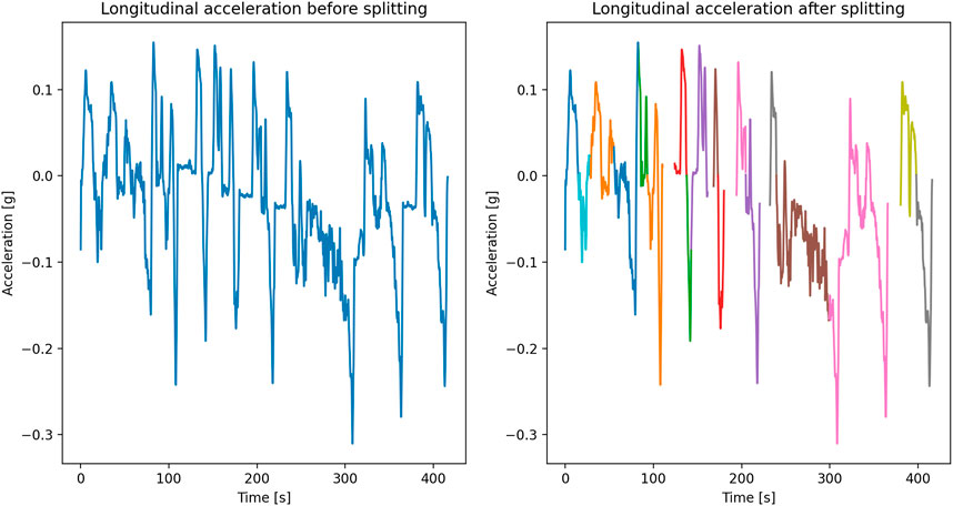
FIGURE 1. Example of a Butterworth filtered acceleration signal before and after splitting for ride no. 1 of an electric vehicle.

FIGURE 2

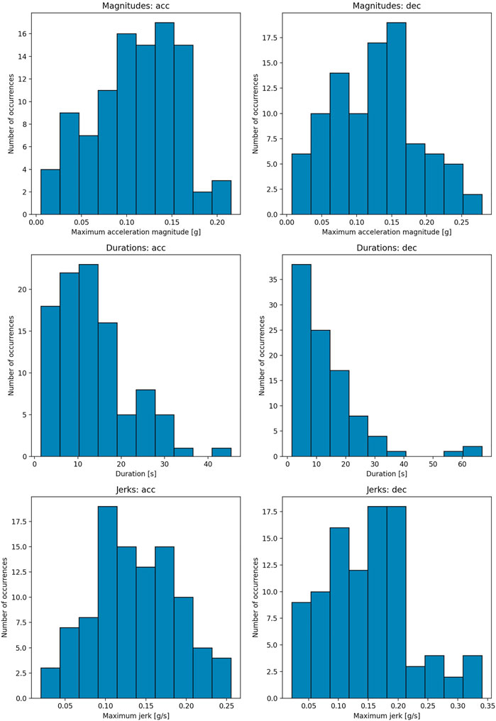
FIGURE 2. Histograms of acceleration magnitudes, peak jerk values and pulse duration for all vehicle types.

For all events under consideration, Legendre expansion up to order N = 10 (i.e., 11 coefficients), N = 50 and N = 200 have been computed.

Mean pulse method and maximum similarity pulses

Both the mean pulse method (constrained and unconstrained) and the maximum similarity method were evaluated as average over all vehicle types (i.e., electric and diesel vehicles) as well as separately for the different types. Figure 3 shows the results of the three methods with all vehicles taken into account, while the results according to vehicle type can be found in the Supplementary Material. Note that the unconstrained mean pulses have been computed with coefficients up to N = 50, while the constrained mean pulses were obtained with a rather rather low (N = 10) number of coefficients. The application of the constrained method only makes sense with such a low number of coefficients; with a higher value of N, the pulses tend to converge to the unconstrained ones with a discontinuity jumping to 0 in the beginning and the end.

FIGURE 3

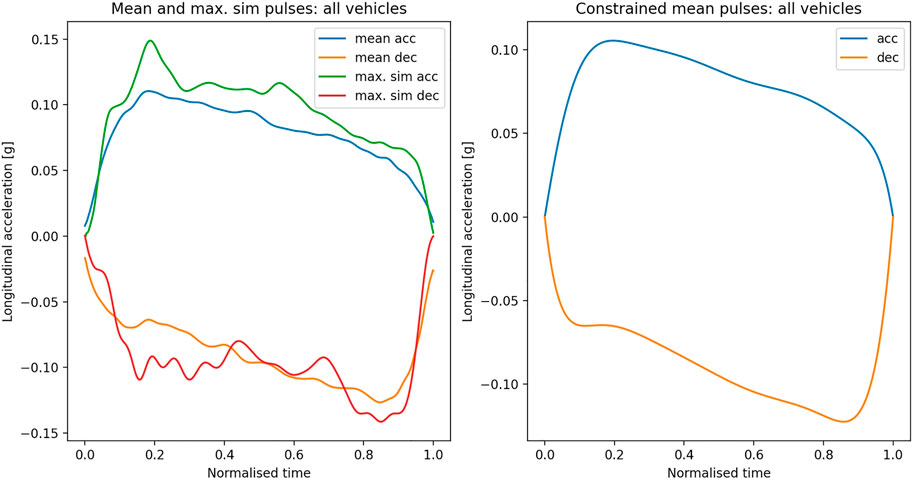
FIGURE 3. Average acceleration and deceleration pulses. Left: computed according to the “unconstrained mean pulse method” (coefficients up to order N = 50) and the “maximum similarity method.” Right: computed according to “constrained mean pulse method” (coefficients up to N = 10). All vehicle types.

The maximum similarity pulses displayed in Figure 3 have been measured on electric vehicles. They do not only represent the pulses of maximum mean similarity overall, but also within the category “electric vehicles.”

As pointed out in the Methods section, the mean pulse methods are only defined up to a constant scaling factor. In the results shown, the scaling was chosen in a way to scale the peak acceleration according to the arithmetic mean of the peak acceleration of the set of pulses under consideration.

Similarity coefficients

While similarity analysis is not the primary focus of this work, sets of similarity coefficients enable the comparison of the performance of the mean pulse and maximum similarity pulse methods. The mean similarity coefficients of the average pulses according to the unconstrained mean pulse method and the maximum similarity method with the full set of ACC and DEC pulses, respectively, are given in Table 1. Furthermore, an evaluation of the similarity coefficients between the mean pulse and the maximum similarity pulse yields 0.9958 (ACC) and 0.984 (DEC). These results have been obtained as averages over all vehicle types.

TABLE 1

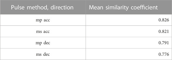
TABLE 1. Mean similarity coefficients of the average pulses according to maximum similarity (ms) and mean pulse (mp) method.

Jerk estimate

For each of the events under consideration, the Legendre coefficients of the jerk time series have been evaluated based on a Legendre representation with 200 coefficients. As an example, the jerk with respect to normalised time is shown for the maximum similarity and (unconstrained) mean pulses in Figure 4. Furthermore, the distribution of the peak jerk values (with respect to time) is presented in Figure 2 for all vehicle types and in Supplementary Figure S7 in the supplementary material separately for the different vehicle types.

FIGURE 4

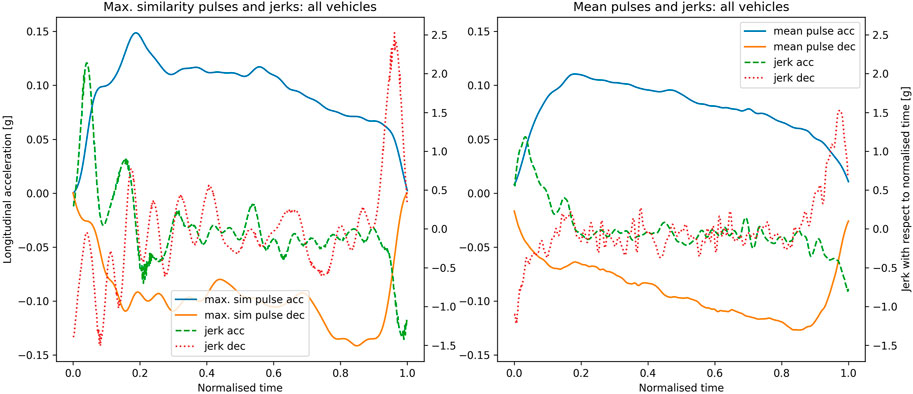
FIGURE 4. Jerk estimates for maximum similarity pulses (left) and unconstrained mean pulses (right), with coefficients up to N = 200 for all vehicle types.

Discussion

In non-collision incidents involving public transportation vehicles, standing passengers are often subjected to balance perturbations due to the acceleration and deceleration of the vehicle. The balance recovery and mitigation of possible injury depend on the perturbation pulse properties, as presented in biomechanical studies (Karekla and Tyler, 2018; Krašna et al., 2021). However, typical bus acceleration and deceleration pulses are difficult to replicate in a laboratory setup. Therefore, for research on the safety of standing passengers, it is essential that the main features of the acceleration and deceleration pulses are properly described. Nevertheless, the research on this topic is scarce compared to research and literature on the safety of, e.g., seated passengers in cars. Kirchner et al. (2014) presented a method of extraction of the pulse characteristics based on Legendre polynomial expansion, which can be considered the current standard and which the method presented here has to be compared to.

Splitting and Lagrange representation

As shown in Figure 1, by using the splitting algorithm, the larger spikes in acceleration and deceleration are consistently detected even though at some points, the trained eye would probably have subdivided some events into several ACC and DEC pulses during manual splitting. This is also apparent from the unequal number of ACC and DEC pulses. However, the more regularly shaped events in the test drive dataset are clearly recognised by the splitting algorithm.

It is clear that manual splitting, as in Kirchner et al. (2014), would improve the quality of pulse splitting in difficult cases. However, an automatic splitting is required as soon as the datasets increase in size. Manual splitting is also used to remove subjective estimates from the analysis. Therefore, we consider it important to develop the splitting algorithm further.

The Legendre representations generally deliver excellent fits of the time-normalised ACC and DEC pulses. With coefficients up to order N = 50 evaluated, an excellent agreement (mean adjusted R² = 0.9987) is reached, while the fits with 11 coefficients reach approximately R² = 0.95. It is dependent upon the application whether a higher accuracy of the fits or a lower number of coefficients is desirable.

Maximum similarity vs mean pulse method

Both the maximum similarity method and the (un)constrained mean pulse method aim at extracting a representative example or average from a number of events with different magnitudes without being dominated by the events with the highest magnitude. The maximum similarity method has been suggested by Kirchner et al. (2014) and can be considered the quasi-standard so far to derive test pulses for laboratory and numerical tests of the postural balance of standing passengers.

The mean pulse method yielded acceleration pulse of average magnitude 0.11 g and deceleration magnitude 0.13 g, while the maximum similarity method resulted in higher pulse magnitudes (Figure 2; Figure 3). This is comparable to the results reported by Kirchner et al. (2014) and Palacio et al. (2009) based on the measured data obtained in a similar setup during regular operation of a city bus, as well as the typical values presented by Kuhn (2013), 0.08–0.11 g for average acceleration and 0.12–0.15 g for deceleration. The peak values occurred at the beginning of the acceleration pulse and at the end of the deceleration pulse, in accordance with experimental observations (Schubert et al., 2017). The peak values of the jerk were 1.0 g/s for acceleration pulse and 1.5 g/s for deceleration pulse in the mean pulse method, while higher values and more noise was observed in the maximum similarity method (Figure 2; Figure 4). Therefore, it can be stated that the mean pulse method captures the key characteristics of the acceleration/deceleration pulses that may be used for representation of balance perturbations for the standing passengers.

Direct comparison of the unconstrained mean pulse and maximum similarity results (Figure 3) shows that the results are surprisingly similar; an observation, which is confirmed by the mutual similarity coefficients $>0.993$. Both methods manage to capture typical features of acceleration and deceleration pulses, such as a strong rise in the beginning followed by a slower decrease and a drop in the end. Also the constrained mean pulses show the typical features, even though in a less detailed way due to the lower order N of the Legendre expansion. The mean similarities of the mean pulse results with the underlying sets are slightly higher than those of the maximums similarity pulses (see Table 1), which reflects the fact that the mean pulse method is based on an optimisation of mean similarity coefficients.

While the maximum similarity method selects one element of the underlying set of pulses, the mean pulse method, when applied to a larger set, converges to a result which 1) is not very sensitive to addition or removal of single pulse from the underlying set and 2) levels out random features of the pulses of the set (average property). Hence, the resulting mean pulses are much smoother than the maximum similarity pulses.

The goal of the mean pulse method is to define test pulses to study the postural balance of standing passengers in presence of acceleration perturbations based on acceleration data sets measured in public transport vehicles. The generation of such test pulses can be done either by applying the mean pulse results directly as test pulses, or by scaling their magnitude to a lower and upper bound to define corridors for the test pulse. In both cases, the convergence and average property of the mean pulse method is an advantage, as similar sets of measured pulses result in similar mean pulses which, furthermore, can be scaled in a meaningful way.

It could be argued that the smoothness of the mean pulses actually is a disadvantage when applied as test pulses for the standing passenger problem, as it could lead to less severe test conditions compared to the spikes and random oscillations observed in the measured acceleration pulses (and, therefore, also in the maximum similarity pulses). Indeed, from the distribution of jerk over time in Figure 4, it is apparent that the maximum similarity pulses do come with higher peak accelerations and jerks. However, the peak values appear at roughly similar times (the peak in the absolute value of the acceleration appears after the first rise, while positive and negative peak jerks appear in the first rise or the last drop). Given that peak jerks and peak accelerations together with the points in time when they appear are the relevant quantities for the severity of an acceleration perturbation to standing passengers (Krašna et al., 2021), the severity of the maximum similarity pulse seems not to be due to the random peaks and oscillations, but rather due to features which are also present in the mean pulses. Therefore, the mean pulses, scaled in time and magnitude to the desired severity, likely provide sufficiently realistic and convenient input to numerical or physical tests, given the advantages discussed above.

Conclusion

In this study, a novel method is presented to define representative average shapes of acceleration and deceleration pulses of public transport vehicles based on measured acceleration time series. This method consists of a combination of automated splitting, Legendre polynomial fits, similarity coefficients and a weighted-mean approach to capture the average shapes without being dominated by events of large magnitude. To test the method and present some pulse shapes as first results, a dataset collected on buses in normal operation was considered, allowing a comparison of the new mean pulse method and the (established) maximum similarity method.

The results show that the proposed method is capable of automatically extracting meaningful representative averages out of the datasets, which due to the weighting are not dominated by the events of the strongest magnitude. Due to the average properties of the method, the mean pulses are free of the random oscillations typically occurring when choosing a representative example out of the set. The proposed method enables the generation of well-defined representative acceleration/deceleration pulses while taking into account the real-life perturbation characteristics observed in field data. The perturbation pulses obtained with the mean pulse method can be applied as scalable test pulses, e.g., in sled experiments with volunteer participants assessing the safety and reaction of standing passengers subject to acceleration/deceleration perturbations. Furthermore, due to the automated splitting algorithm, the method can be applied also to larger datasets and mean pulses representative of more exhaustive data can be generated in a straightforward way.

The newly emerging finite element human body models capable of replicating standing passengers will likely offer a particularly interesting application of the mean pulse method: with these models, also higher severity perturbations with increased injury risk can be tested. The test pulses for these can be obtained from the mean pulse method, either by scaling the existig pulses or by applying it to field data sets containing emergency driving manoeuvres.

Data availability statement

The datasets presented in this study can be found in online repositories. The names of the repository/repositories and accession number(s) can be found below: OpenVT platform: https://openvt.eu/Acceleration_data_and_tools.

Author contributions

AK developed the concept of the average pulse method and contributed to the data analysis. SK contributed to the data analysis. Both authors contributed equally to writing the article.

Funding

This work has been created as part of project VIRTUAL and has received funding from the European Union’s Horizon 2020 research and innovation programme under grant agreement No 768960.

Acknowledgments

The authors would like to thank Jakob Gross (AGU Zürich) for carrying out the measurements of bus accelerations and Markus Muser and Kai-Uwe Schmitt (both AGU Zürich) for helpful discussions and ideas. Furthermore, we would like to thank two reviewers for constructive comments and valuable input.

Conflict of interest

AK was employed by AGU Zürich.

The remaining author declares that the research was conducted in the absence of any commercial or financial relationships that could be construed as a potential conflict of interest.

Publisher’s note

All claims expressed in this article are solely those of the authors and do not necessarily represent those of their affiliated organizations, or those of the publisher, the editors and the reviewers. Any product that may be evaluated in this article, or claim that may be made by its manufacturer, is not guaranteed or endorsed by the publisher.

Supplementary material

The Supplementary Material for this article can be found online at: https://www.frontiersin.org/articles/10.3389/ffutr.2023.931780/full#supplementary-material

Footnotes

¹https://openvt.eu/Acceleration_tools/Bus_data_and_tools.

²By definition, for ACC events, the cumulative acceleration is $>0$, while for DEC events, the cumulative acceleration is negative.

³Of course, the sets can also be re-combined in different ways—we leave it to the reader to come up with suitable indexing in this case. In places where only the pulses of one set (e.g., one ACC set) are compared with each other, we will drop the identifier I altogether to make the notation less clumsy.

⁴According to Hale and Townsend (2016), it would be possible to further speed up this computation by using a method similar to the fast Fourier transformation. This approach could be a good way to make the method more suitable for larger data quantities.

⁵According to Lu et al. (2013), this method performs significantly better than the finite differences scheme and even has advantages over approaches based on polynomial interpolation.

⁶It could potentially be that this definition is not unique—that is, that there are two pulses with the same mean similarity coefficient. This is, however, unlikely in measured acceleration pulses.

⁷Note that, as opposed to the previous sections, where given time-normalised acceleration pulses were approximated and analysed in Legendre series, we take the opposite approach now and define a new pulse by defining its Legendre coefficients.

⁸The mean similarity coefficient of this pulse is by construction ≥ that of the maximum similarity pulse, as the maximum similarity pulse is the pulse within the given set which has the highest mean similarity coefficient, while the mean pulse manifests the highest mean similarity coefficient theoretically possible in any Legendre expanded pulse of order N.

⁹Given that the similarity coefficient is invariant with respect to re-scaling the coefficients, we denote the mean similarity coefficient $\bar{s}$ with the same symbol whether it is meant as a function of the coefficient c_k or the coefficient α_k.

References

Aftab, Z., Robert, T., and Wieber, P.-B. (2016). Balance recovery prediction with multiple strategies for standing humans. PLOS ONE 11, 1–16. doi:10.1371/journal.pone.0151166

CrossRef Full Text | Google Scholar

Brooks, B., Edwards, H., Fraser, C., Levis, J., and Johnson, M. (1978). “Passenger problems on moving buses,” in Mobility for the Elderly and the Handicapped. The International Conference on Transport for the Elderly and Handicapped. Loughborough University of Technology Florida State University, Tallahassee.

Google Scholar

Carpenter, M. G., Thorstensson, A., and Cresswell, A. G. (2005). Deceleration affects anticipatory and reactive components of triggered postural responses. Exp. brain Res. 167, 433–445. doi:10.1007/s00221-005-0049-3

PubMed Abstract | CrossRef Full Text | Google Scholar

Elvik, R. (2019). Risk of non-collision injuries to public transport passengers: Synthesis of evidence from eleven studies. J. Transp. Health 13, 128–136. doi:10.1016/j.jth.2019.03.017

CrossRef Full Text | Google Scholar

European Commission (2022). Annual statistical report on road safety in the EU, 2021 (European road safety observatory. Brussels, European commission, directorate general for transport).

Google Scholar

Graaf, B. D., and Van Weperen, W. (1997). The retention of blance: An exploratory study into the limits of acceleration the human body can withstand without losing equilibrium. Hum. factors 39, 111–118. doi:10.1518/001872097778940614

PubMed Abstract | CrossRef Full Text | Google Scholar

Hale, N., and Townsend, A. (2016). A fast FFT-based discrete Legendre transform. IMA J. Numer. Analysis 36, 1670–1684. doi:10.1093/imanum/drv060

CrossRef Full Text | Google Scholar

Halpern, P., Siebzehner, M., Aladgem, D., Sorkine, P., and Bechar, R. (2005). Non-collision injuries in public buses: A national survey of a neglected problem. Emerg. Med. J. 22, 108–110. doi:10.1136/emj.2003.013128

PubMed Abstract | CrossRef Full Text | Google Scholar

Hoberock, L. L. (1977). A survey of longitudinal acceleration comfort studies in ground transportation vehicles. J. Dyn. Syst. Meas. Control 99, 76–84. doi:10.1115/1.3427093

CrossRef Full Text | Google Scholar

Karekla, X., and Tyler, N. (2018). Reducing non-collision injuries aboard buses: Passenger balance whilst walking on the lower deck. Saf. Sci. 105, 128–133. doi:10.1016/j.ssci.2018.01.021

CrossRef Full Text | Google Scholar

Kendrick, D., Drummond, A., Logan, P., Barnes, J., and Worthington, E. (2015). Systematic review of the epidemiology of non-collision injuries occurring to older people during use of public buses in high income countries. J. Transp. Health 2, 394–405. doi:10.1016/j.jth.2015.06.002

CrossRef Full Text | Google Scholar

Kirchner, M., Schubert, P., and Haas, C. T. (2014). Characterisation of real-world bus acceleration and deceleration signals. J. Signal Inf. Process. 5, 8–13. doi:10.4236/jsip.2014.51002

CrossRef Full Text | Google Scholar

Kirk, A., Grant, R., and Bird, R. (2003). “Passenger casualties in non-collision incidents on buses and coaches in great Britain,” in Proceedings of the 18th International Technical Conference on the Enhanced Safety of Vehicles, May 2003 (Nagoya, Japan), 19–22. Available at: https://www-nrd.nhtsa.dot.gov/departments/esv/18th/

Google Scholar

Krašna, S., Keller, A., Linder, A., Silvano, A. P., Xu, J.-C., Thomson, R., et al. (2021). Human response to longitudinal perturbations of standing passengers on public transport during regular operation. Front. Bioeng. Biotechnol. 9, 680883. doi:10.3389/fbioe.2021.680883

PubMed Abstract | CrossRef Full Text | Google Scholar

Kuhn, W. (2013). Fundamentals of road design. Southampton, United Kingdom: WIT Press.

Google Scholar

Li, D., Zhao, Y., Bai, Q., Zhou, B., and Ling, H. (2017). Analyzing injury severity of bus passengers with different movements. Traffic Inj. Prev. 18, 528–532. doi:10.1080/15389588.2016.1262950

PubMed Abstract | CrossRef Full Text | Google Scholar

Lu, S., Naumova, V., and Pereverzev, S. V. (2013). Legendre polynomials as a recommended basis for numerical differentiation in the presence of stochastic white noise. J. Inverse Ill-posed Problems 21, 193–216. doi:10.1515/jip-2012-0050

CrossRef Full Text | Google Scholar

McKinney, W. (2010). “Data structures for statistical computing in python,” in Proceedings of the 9th Python in science conference. Editors S. van der Walt, and J. Millman, 51–56.

CrossRef Full Text | Google Scholar

Morency, P., Strauss, J., Pépin, F., Tessier, F., and Grondines, J. (2018). Traveling by bus instead of car on urban major roads: Safety benefits for vehicle occupants, pedestrians, and cyclists. J. urban health 95, 196–207. doi:10.1007/s11524-017-0222-6

PubMed Abstract | CrossRef Full Text | Google Scholar

Palacio, A., Tamburro, G., O’Neill, D., and Simms, C. K. (2009). Non-collision injuries in urban buses—Strategies for prevention. Accid. Analysis Prev. 41, 1–9. doi:10.1016/j.aap.2008.08.016

PubMed Abstract | CrossRef Full Text | Google Scholar

Paton, K. (1975). Picture description using Legendre polynomials. Comput. Graph. Image Process. 4, 40–54. doi:10.1016/0146-664x(75)90020-9

CrossRef Full Text | Google Scholar

Phillips, T. N. (1988). On the Legendre coefficients of a general-order derivative of an infinitely differentiable function. IMA J. Numer. Analysis 8, 455–459. doi:10.1093/imanum/8.4.455

CrossRef Full Text | Google Scholar

Powell, J., and Palacín, R. (2015). Passenger stability within moving railway vehicles: Limits on maximum longitudinal acceleration. Urban Rail Transit 1, 95–103. doi:10.1007/s40864-015-0012-y

CrossRef Full Text | Google Scholar

Robert, T., Beillas, P., Maupas, A., and Verriest, J.-P. (2007). Conditions of possible head impacts for standing passengers in public transportation: An experimental study. Int. J. crashworthiness 12, 319–327. doi:10.1080/13588260701433552

CrossRef Full Text | Google Scholar

Schubert, P., Liebherr, M., Kersten, S., and Haas, C. T. (2017). Biomechanical demand analysis of older passengers in a standing position during bus transport. J. Transp. Health 4, 226–236. doi:10.1016/j.jth.2016.12.002

CrossRef Full Text | Google Scholar

Tokuno, C. D., Cresswell, A. G., Thorstensson, A., and Carpenter, M. G. (2010). Age-related changes in postural responses revealed by support-surface translations with a long acceleration–deceleration interval. Clin. Neurophysiol. 121, 109–117. doi:10.1016/j.clinph.2009.09.025

PubMed Abstract | CrossRef Full Text | Google Scholar

Turkovich, M. J., Van Roosmalen, L., Hobson, D. A., and Porach, E. A. (2011). The effect of city bus maneuvers on wheelchair movement. J. Public Transp. 14, 147–169. doi:10.5038/2375-0901.14.3.8

CrossRef Full Text | Google Scholar

Virtanen, P., Gommers, R., Oliphant, T. E., Haberland, M., Reddy, T., Cournapeau, D., et al. (2020). SciPy 1.0: Fundamental algorithms for scientific computing in Python. Nat. Methods 17, 261–272. doi:10.1038/s41592-019-0686-2

PubMed Abstract | CrossRef Full Text | Google Scholar

Wang, H., and Xiang, S. (2012). On the convergence rates of Legendre approximation. Math. Comput. 81, 861–877. doi:10.1090/s0025-5718-2011-02549-4

CrossRef Full Text | Google Scholar

Zaworski, J. R., Hunter-Zaworski, K., and Baldwin, M. (2007). Bus dynamics for mobility-aid securement design. Assist. Technol. 19, 200–209. doi:10.1080/10400435.2007.10131877

PubMed Abstract | CrossRef Full Text | Google Scholar