 Victor Tkachev1
 Maxim Sorokin1,2
 Artem Mescheryakov3
 Alexander Simonov1
 Andrew Garazha1
 Anton Buzdin1,2,4
 Ilya Muchnik5
 Nicolas Borisov1,4*
- 1Department of Bioinformatics and Molecular Networks, OmicsWay Corporation, Walnut, CA, United States
- 2Shemyakin-Ovchinnikov Institute of Bioorganic Chemistry, Moscow, Russia
- 3Yandex N.V. Corporation, Moscow, Russia
- 4I.M. Sechenov First Moscow State Medical University (Sechenov University), Moscow, Russia
- 5Hill Center, Rutgers University, Piscataway, NJ, United States
Here, we propose a heuristic technique of data trimming for SVM termed FLOating Window Projective Separator (FloWPS), tailored for personalized predictions based on molecular data. This procedure can operate with high throughput genetic datasets like gene expression or mutation profiles. Its application prevents SVM from extrapolation by excluding non-informative features. FloWPS requires training on the data for the individuals with known clinical outcomes to create a clinically relevant classifier. The genetic profiles linked with the outcomes are broken as usual into the training and validation datasets. The unique property of FloWPS is that irrelevant features in validation dataset that don’t have significant number of neighboring hits in the training dataset are removed from further analyses. Next, similarly to the k nearest neighbors (kNN) method, for each point of a validation dataset, FloWPS takes into account only the proximal points of the training dataset. Thus, for every point of a validation dataset, the training dataset is adjusted to form a floating window. FloWPS performance was tested on ten gene expression datasets for 992 cancer patients either responding or not on the different types of chemotherapy. We experimentally confirmed by leave-one-out cross-validation that FloWPS enables to significantly increase quality of a classifier built based on the classical SVM in most of the applications, particularly for polynomial kernels.
Introduction
Support vector machine is one of the most popular machine learning methods in biomedical sciences with constantly growing impact and more than 11,000 citations in the PubMed-indexed literature1, of those ∼2,300 are only for the 2017 and first 6 months of 2018. This method has been successfully applied for a wide variety of biomedical applications like searching Dicer RNase cleavage sites on pre-miRNA (Ahmed et al., 2013), prediction of miRNA guide strands (Ahmed et al., 2009a), identification of poly(A) signals in genomic DNA (Ahmed et al., 2009b), finding conformational B-cell epitopes in antigens by nucleotide sequence (Ansari and Raghava, 2010). More recent developments include drug design according to physicochemical properties (Yosipof et al., 2018), learning on transcriptomic profiles for age recognition (Mamoshina et al., 2018), predictions of drug toxicities and other side effects (Zhang et al., 2018).
The performance quality of the classifiers based on these methods may reach the value of 0.80 or higher for the metrics such as ROC AUC2 and/or accuracy rate, e.g., for problems of age recognition (Mamoshina et al., 2018) and drug compound selection (Yosipof et al., 2018). However, although generally clearly helpful, the SVM approach frequently demonstrates insufficient performance in several applications for separating groups of the patients with different clinical outcomes (Mulligan et al., 2007; Ray and Zhang, 2009; Babaoglu et al., 2010; Kim et al., 2018). These failures were most likely caused by insufficient number of preceding clinical cases, which provokes overtraining of all machine learning algorithms. Particularly, the rareness of training points in the feature space leads to frequent extrapolations, and SVM method is known to be highly vulnerable to such conditions (Arimoto et al., 2005; Balabin and Lomakina, 2011; Balabin and Smirnov, 2012; Betrie et al., 2013).
In order to increase the performance of SVM for distinguishing between clinically relevant features, such as degrees of response to cancer therapies, we propose here a new method termed FloWPS for data trimming that generalizes the SVM technique by precluding extrapolation in the feature space. FloWPS acts by selecting for further analysis only those features that lay within the intervals of data projections from the training dataset. This approach can avoid extrapolations in favor of interpolations and thus increases a prediction quality of the output data. FloWPS combines somehow two methods, SVM and kNN (Altman, 1992), where kNN plays a particular role to extract informative features. The idea to combine feature extraction methods with SVM is well known (Tan and Gilbert, 2003; Kourou et al., 2015; Tan, 2016; Liu et al., 2017; Tarek et al., 2017). The approach proposed in this paper, however, is in principle a novelty, at least because its selection capacity is focused on every single point available for prediction.
We tested FloWPS on ten published gene expression datasets for totally 992 cancer patients treated with different types of chemotherapy with known clinical outcomes. In all the cases, the classifiers built using FloWPS outperformed standard SVM classifiers.
Results
Data Sources and Feature Selection
In this study, we investigated gene expression features associated with the responses to chemotherapy. The gene expression profiles were extracted from the datasets summarized in Table 1. The clinical outcome information was related to response on different chemotherapy regimens, linked with high throughput gene expression profiles for the individual patients.
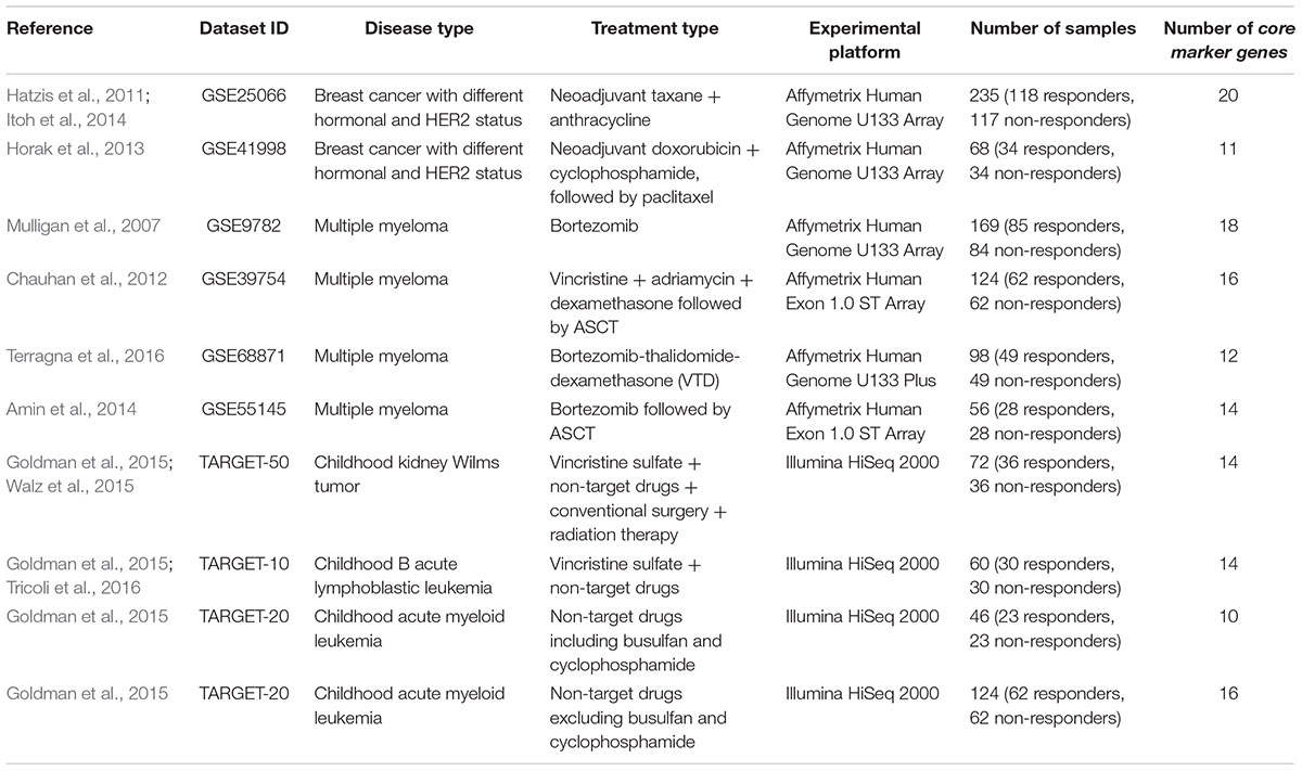
Table 1. Clinically annotated gene expression datasets.
Each patient was primarily labeled as either responder or non-responder to a treatment. For all the datasets taken from the GEO repository, we used the response criteria formulated in the respective original papers first publishing these data. Namely, for two breast cancer datasets, GSE25066 (Hatzis et al., 2011; Itoh et al., 2014) and GSE41998 (Horak et al., 2013), we considered partial responders as responders. For the first multiple myeloma dataset, GSE9782 (Mulligan et al., 2007), we took the (non)responder classification used by the authors, where patents with complete and partial response were annotated as responders, and with no change and progressive disease – as non-responders. For three other multiple myeloma datasets, GSE39753 (Chauhan et al., 2012), GSE68871 (Terragna et al., 2016), and GSE55145 (Amin et al., 2014), we considered complete, near-complete and very good partial responders as responders, whereas partial, minor and worse responders – as non-responders. For the datasets of pediatric Wilms kidney tumor, ALL and AML, extracted from the TARGET gene expression repository of National Cancer Institute (Goldman et al., 2015), the cases was classified according the distribution of the event-free survival time, which appeared to have two modes with different slopes (Supplementary Figure S1).
To preclude any possible bias that may affect the performance of machine-learning classifiers due to unequal representation of samples in two different classes (clinical responders and non-responders), numbers of responding and non-responding cases were equalized within each dataset. Equalization was done by taking the full smaller subset of those for the two classes (responders/non-responders), and then by random selection of samples from the bigger subset. Thus, each resulting dataset contained equal numbers of cases classified as responders and non-responders.
To engineer a plausible feature space, where the SVM can be applied efficiently, we proposed to select from tens of thousands of individual gene expression features only few of them, which produce a good separation of clinical responders from non-responders. To do so, for every dataset under investigation we selected its particular top 30 genes, whose expression levels taken one by one had the highest ROC AUC values for distinguishing responder and non-responder profiles. We made a number of top informative features equal to 30 because the usual number of samples in considered datasets was not lower than 50 (a direct heuristic number for degree of freedom). These 30 top marker genes, and response statuses (100 for a responder, 0 for a non-responder) for all selected patients from all datasets are listed on Supplementary Table S1.
To produce more robust feature selection, for each dataset having, say, N samples, the leave-one-out procedure has been performed. Each individual sample was removed from the investigation one at a time, so N subdatasets each having N-1 individuals were generated. For each subdataset, the ROC AUC test was performed between responders and non-responders for each gene. The genes were next sorted according to their ROC AUC, and top 30 were selected for each subdataset. The final list of such core informative genes was generated as an intersection between top 30 selected genes for all N subdatasets. For every dataset under investigation, these final core sets are listed in Supplementary Table S2; the number of core marker genes is also shown on Table 1.
Data Trimming for Application in SVM
We developed a first of its class data trimming3 tool termed FloWPS that has a potential to improve the performance of machine learning methods. Since extrapolation is a widely recognized Achilles heel of SVM (Arimoto et al., 2005; Balabin and Lomakina, 2011; Balabin and Smirnov, 2012; Betrie et al., 2013), FloWPS avoids it by using the rectangular projections along all irrelevant expression features that cause extrapolation during the SVM-based predictions for every validation point.
In this section we describe and investigate our data trimming procedure (FloWPS) as a preprocessing for SVM application.
Since the number of samples in most of the datasets used here was relatively low, we tested our classifier using the leave-one-out cross-validation method, which introduces lesser errors than the standard five-bin cross-validation scheme generally applied for bigger datasets. According to the leave-one-out approach, for each sample i = 1, N serves as a validation case whose response to the treatment had to be predicted, whereas all remaining samples, j = 1,…(i-1),(i+1),…,N, collectively acts as a training dataset, and this procedure is repeated for all the samples. For machine leaning without data trimming, in a predefined feature space F = (f1,…, fs ) every sample i, given for the test, is assigned by a classifier, constructed to (N-1) samples used for training.
According to the current data trimming approach, instead a fixed space F for all N testing samples, we propose using an individual space Fi, which contains individually adapted training data (of N-1 samples) for the testing sample i. It can be implemented using the following heuristics (Figure 1).
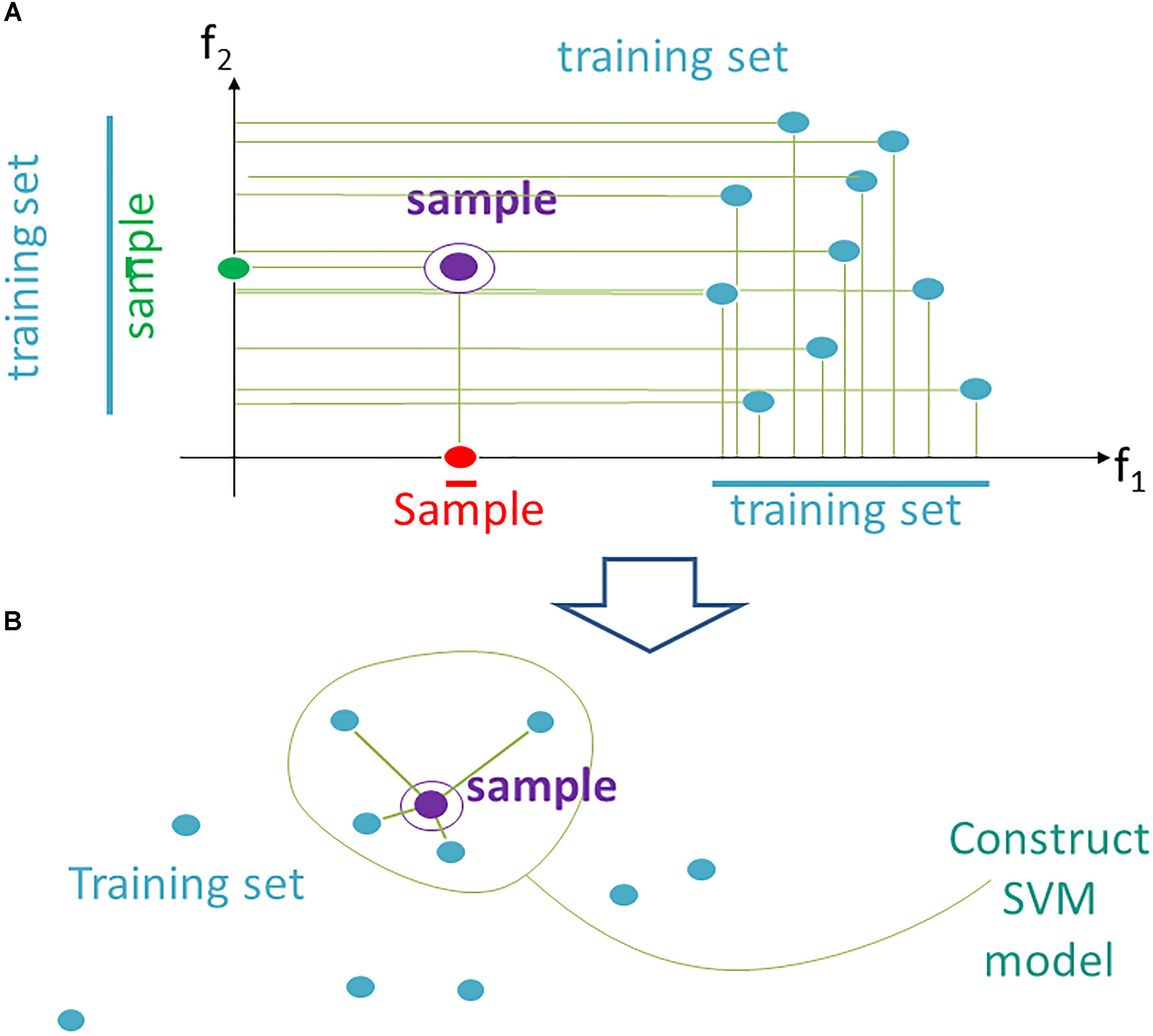
Figure 1. Data trimming pipeline. (A) selection of relevant features in FloWPS according to the m-condition. A violet dot shows the position of a validation point. Turquoise dots stand for the points from the training dataset. The features (here: f1 and f2) are considered relevant when they satisfy the criterion that at least m flanking training points must be present on both sides relative to the validation point along the feature-specific axis. In the figure, it is exemplified that m-condition is satisfied for f1 feature when m = 0 only, and for the f2, when m ≤ 5. (B) After selection of the relevant features, only k nearest neighbors in the training sets are selected to construct the SVM model. On the figure, k = 4, although k starting from 20 was used in our calculations, to build SVM model.
(1) From the whole predefined feature space F = (f1,…, fs ) we extract a subset Fi (m), where m is a parameter. A feature fj is kept in Fi(m) if on its axis there are at least m projections from training samples, which are larger than fj (i), and, at the same time, at least m, which are smaller than fj (i). The procedure for extraction of a subset Fi(m) is illustrated in Figure 1A for a two-dimensional space F = (f1, f2). A violet point stands for the validation sample in the feature space. Turquoise dots represent scattering of the training points. For example, the m-condition for the feature f2 is satisfied when m = 0,1,2,3,4,5 (projection of the training set on f2 axis has five points both below and above the validation point), whereas for the feature f1 it is satisfied only for m = 0 (projection of the validation point on axis f1 lies outside of the cloud of training points).
(2) In Fi (m) we keep for training only k closest samples (from given (N-1) samples); k is also a parameter (Figure 1B; note that although for the sake of simplicity k = 4 in the picture, in the computational trials we varied k from 20 to N-1).
Hence, for every individual i = 1, N, and m and k parameter values, the predicted classification values are obtained [i.e., predictions Pi (m,k), i = 1, N]. Considering known response status for each sample i, it is possible to calculate AUC values for a whole set of samples as a function over whole range of the parameters m and k (Figure 2B). Since the predicted classification efficiencies depend upon the chosen values for m and k, it is possible to interrogate the AUC values over the full lattice of all possible (m, k) pairs.
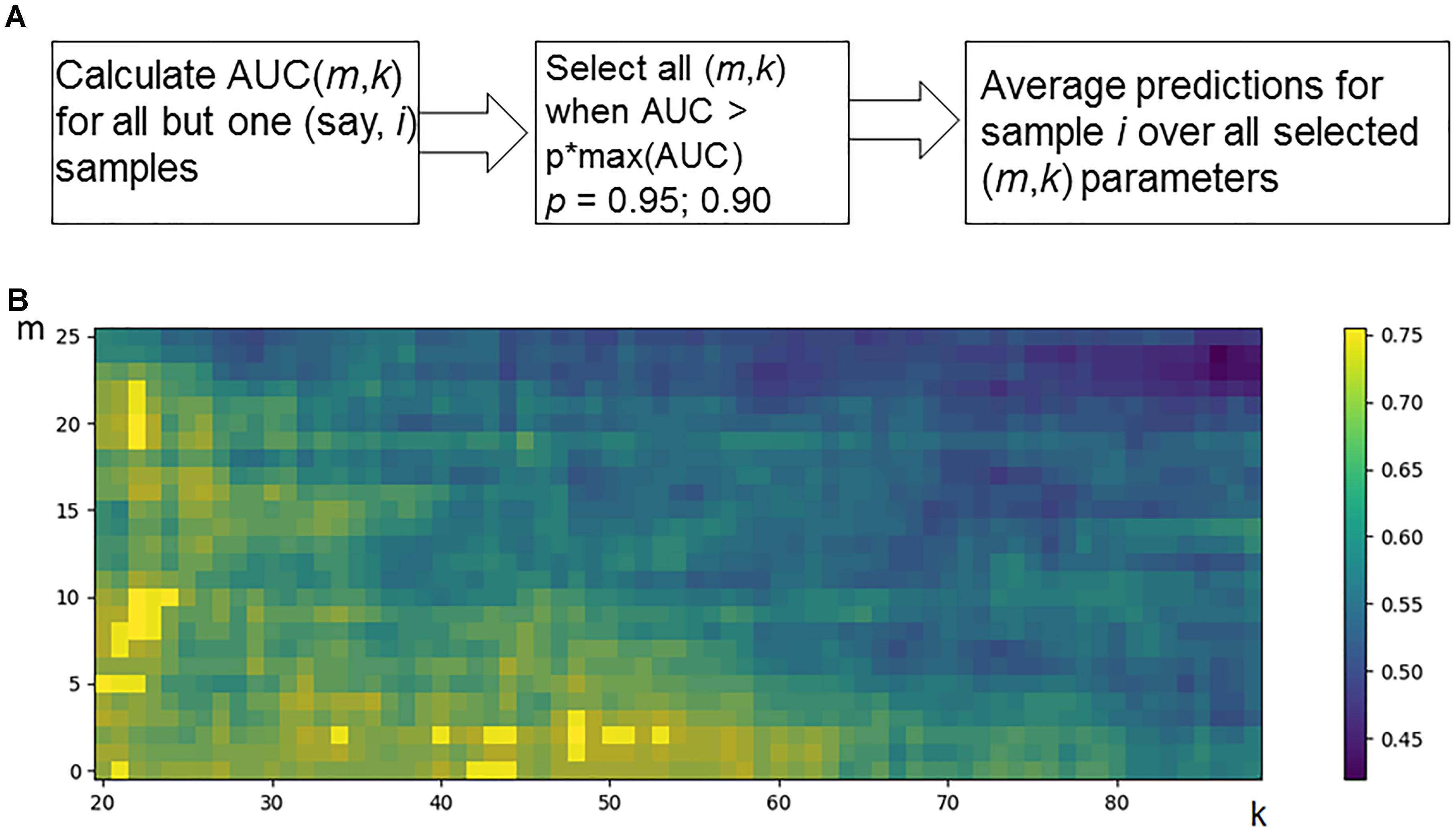
Figure 2. Optimization of data trimming parameters m and k for a given individual. (A) Overall scheme for prediction for an individual sample i = 1, N. All but one individuals serve as a training dataset. For a training dataset at the fitting step, the AUC for a classifier prediction is calculated and plotted (B) as a function of data trimming parameters m and k. Positions of this AUC topogram where AUC > p ⋅ max(AUC), p = 0.95, are considered prediction-accountable (highlighted with bright yellow color) and form the prediction-accountable set S. This AUC topogram, as well as the set S, is individual for every validation point i.
We propose an algorithm of achieving the optimal (m,k)-settings for a final classifier (Figure 2A). The AUC threshold (θ) is set to 𝜃 = p ⋅ max(AUC), where max(AUC) is the maximal value of AUC, taken over the set of all possible (m, k) pairs, and the parameter p equals to a user-defined confidence threshold. To illustrate performance of this approach, we took two alternative values of p = 0.95 or 0.90, and then considered all the (m,k) pair positions on the AUC(m,k) topogram. We next screened for the positions where AUC exceeded the threshold θ, and the total combination of these positions was taken as the prediction-accountable set S (Figure 2B; prediction-accountable positions are shown in yellow). The final prediction of FloWPS (PF) for a certain validation case should be calculated by averaging the SVM predictions, P(m,k), over the whole set of positions belonging to the prediction-accountable set S, according to the formula: PF = meanS(P(m,k)).
The usual SVM method, i.e., without FloWPS data trimming, corresponds to a very right and bottom corner of the AUC(m,k) topogram (Figure 2B), with the parameter settings m = 0, k = N - 1. On the example shown in Figure 2B, the classical SVM, without any doubt, provides essentially lower accuracy than FloWPS.
FloWPS Performance for Default SVM Settings
At first, we investigated performance of FloWPS on ten cancer gene expression datasets (Table 1) with the default SVM settings (linear kernel and cost/penalty parameter C = 1). During our calculations, the FloWPS classifier was first fitted for the training dataset without a sample (say, i) to be classified. For these all (N-1) samples AUCi(m,k) was calculated as a function of data trimming parameters m and k (see Figure 2A). This enabled finding the prediction-accountable set Si in the AUCi(m,k) topogram (on Figure 2B, the set was marked with bright yellow). The m and k values from the set Si were then used for data trimming and classifying of a single sample i. In parallel, we applied the standard SVM algorithm for leave-one-out cross-validation without data trimming, i.e., m = 0, k = N-1 for each training sub-dataset. The comparison is shown on Table 2, Supplementary Table S3, and Figures 3, 4.
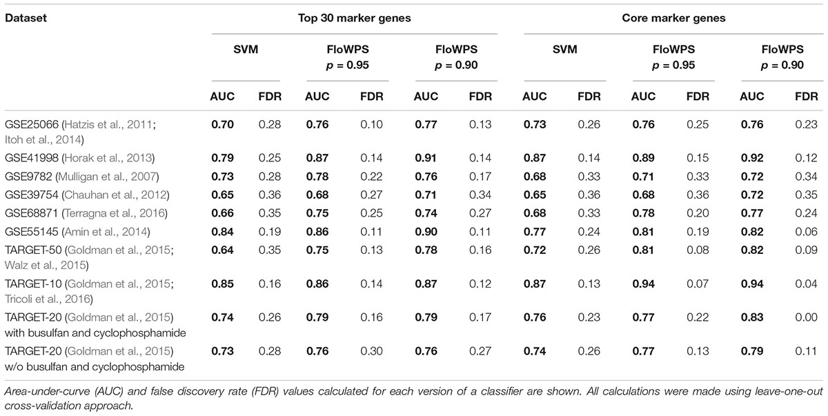
Table 2. Performance of clinical response classifiers for clinically annotated gene expression datasets.
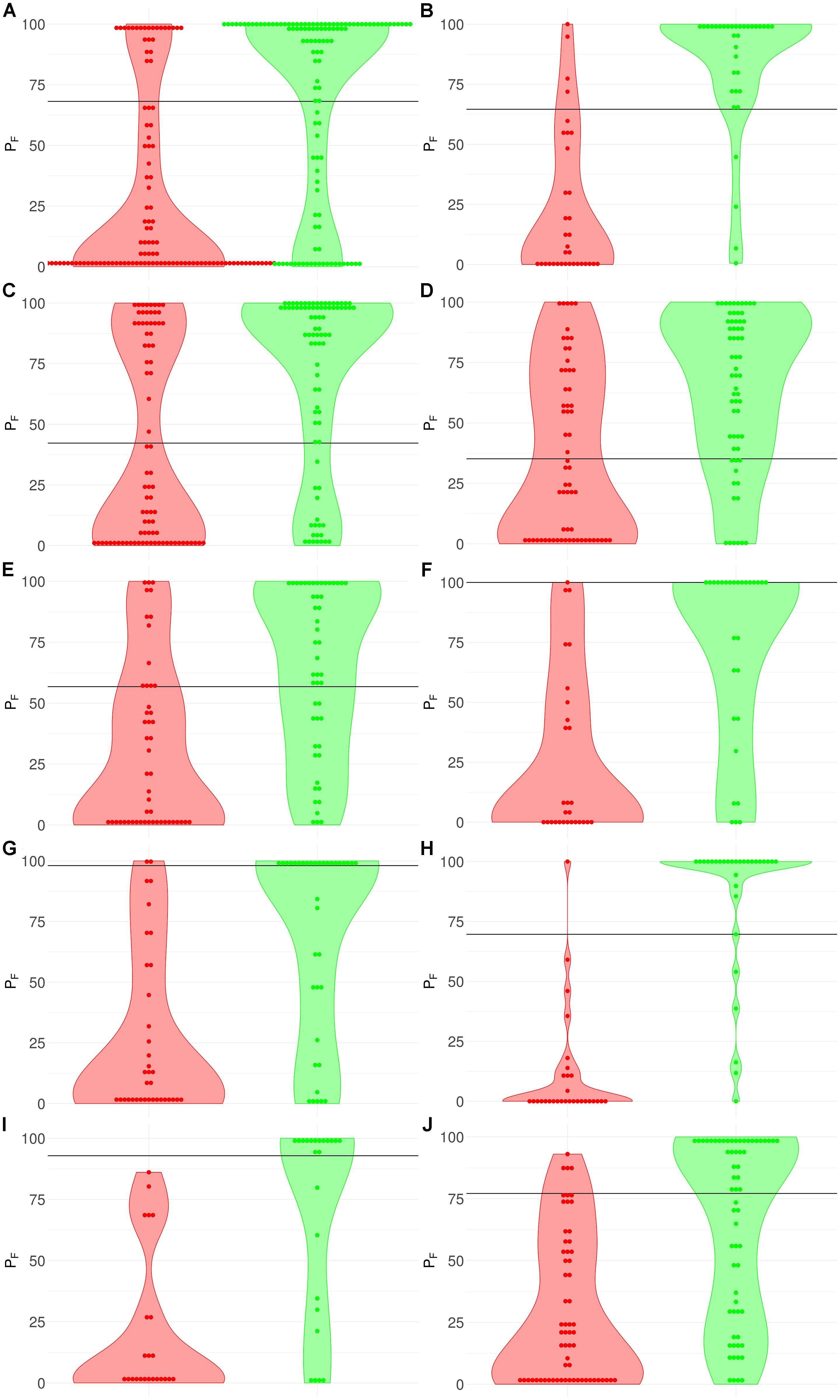
Figure 3. Distribution (violin plots together with each instance showed as a red/green dot) of FloWPS predictions (PF) for patients without (red plots and dots) and with (green plots and dots) positive clinical response to chemotherapy treatment. For FloWPS, core marker genes and p = 0.90 settings were used. Black horizontal line shows the discrimination threshold (τ) between responders and non-responders for each classifier. Panels represent different data sources, (A) GSE25066; (B) GSE41998; (C) GSE9782; (D) GSE39754; (E) GSE68871; (F) GSE55134; (G) TARGET-50; (H) TARGET-10; (I) and (J): TARGET-20 with and without busulfan and cyclophosphamide, respectively.
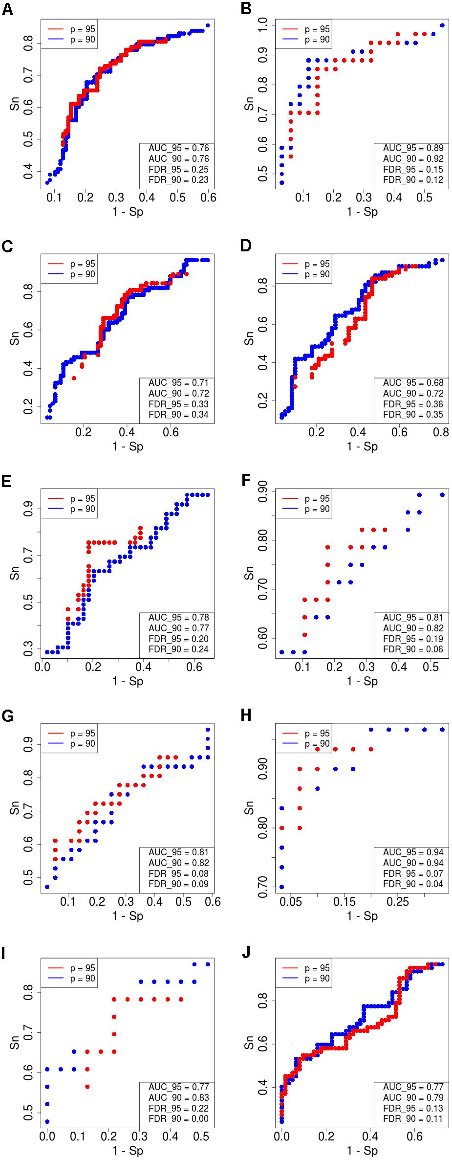
Figure 4. Receiver–operator curves (ROC) showing the dependence of sensitivity (Sn) upon specificity (Sp) for FloWPS-based classifier of treatment response for datasets with core marker genes. Red dots: confidence parameter p = 0.95, blue dots: p = 0.90. Panels represent different clinically annotated datasets, (A) GSE25066; (B) GSE41998; (C) GSE9782; (D) GSE39754; (E) GSE68871; (F) GSE55134; (G) TARGET-50; (H) TARGET-10; (I,J) TARGET-20 with and without busulfan and cyclophosphamide, respectively.
The discrimination threshold (τ), which is shown as a black horizontal line on Figure 3 (so that any sample with FloWPS prediction value above τ is classified as a responder, and below it – as a non-responder), was set to minimize the sum of FP and FN predictions.
For every dataset, confidence parameter p and scheme of gene selection, FloWPS classifier demonstrated the ROC AUC exceeding the corresponding value for the classical SVM (Table 2). For three datasets out of ten, AUC for classical SVM was between 0.64 and 0.68. For all these cases, application of FloWPS with confidence level p = 0.90 enabled obtaining essentially better AUC values ranging between 0.71 and 0.78.
The comparison of classifier’s quality by another metric, the FDR4, has demonstrated similar results: FDR was lower for FloWPS than for classical SVM for almost all the cases (Table 2, columns without boldface font). Other metrics, such as sensitivity (Sn), specificity (Sp), accuracy rate (ACC) and MCC5 also strongly tend to be higher for FloWPS than for classical SVM without data trimming (Supplementary Table S3).
FloWPS Performance at Different Settings and Comparison With Alternative Data Reduction Approach
Although the classifier quality tended to be higher for data trimming than for default SVM settings, the advantages were different in different cancer datasets. The FloWPS performance, therefore, was investigated for different SVM kernels (linear vs. polynomial) and different values for cost/penalty parameters C (ranged from 0.1 to 1000), Figure 5 and Supplementary Table S4. These calculations were done for the core marker gene datasets and FloWPS confidence parameter p = 0.90. The advantage of FloWPS over SVM is more essential in the conditions vulnerable to SVM overtraining, e.g., for linear kernel with high values of the cost/penalty parameter (C = 100 or 1000) or for polynomial kernel, where SVM may be easily overfitted. Fortunately, FloWPS precludes such overfitting, thus raising AUC and decreasing FDR. The same pattern was also seen for the Sn, Sp, ACC and MCC values (Supplementary Table S4).
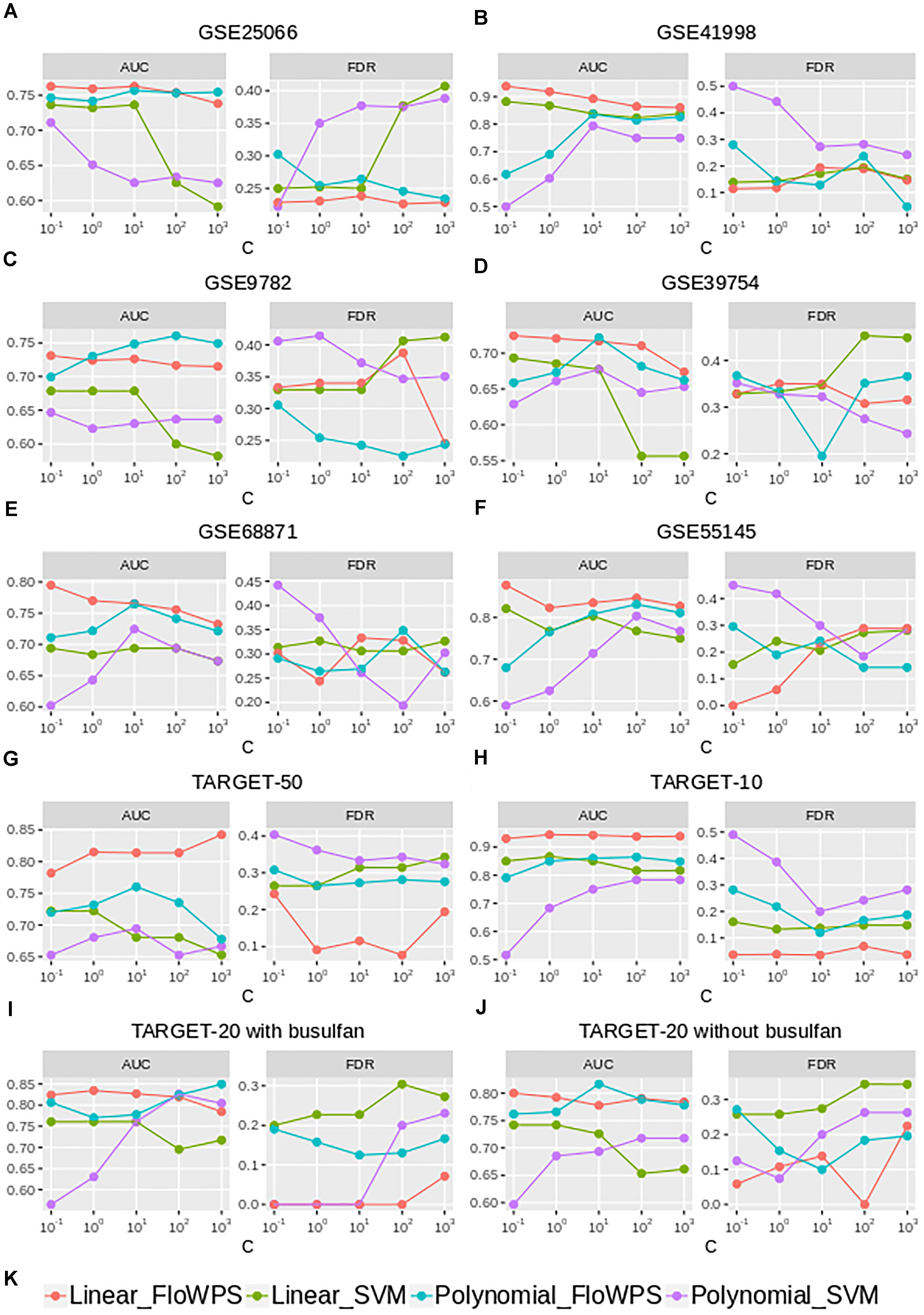
Figure 5. AUC and FDR for (non)responders classifier as a function of cost/penalty parameter C for classical SVM (without data trimming) and FloWPS for both linear and polynomial kernels. Calculations were done for core marker gene datasets and confidence parameter p = 0.90. Different panels represent different datasets, (A) GSE25066; (B) GSE41998; (C) GSE9782; (D) GSE39754; (E) GSE68871; (F) GSE55134; (G) TARGET-50; (H) TARGET-10; (I,J) TARGET-20 with and without busulfan and cyclophosphamide, respectively. (K) Legend showing FloWPS and SVM modifications.
Note that FloWPS is not the only possible data reduction/feature selection method, which may be used for preprocessing to improve the classifier’s quality. To try a simple alternative to FloWPS, which is, however, not specific to individual samples, we did calculations based on PCA mode rather than original features. The number of PCs taken for building the SVM model, may act as a parameter, which is optimized in a manner similar to optimization of m and k for FloWPS. Namely, a maximum for AUC as a function of PC number is found and then used as the optimal number of PCs for an SVM-based prediction.
Thus, we compared the classifier qualities for three methods, namely classical SVM without data reduction, PCA-assisted SVM with pre-trained PC number, and FloWPS with the confidence parameter p = 0.90 (Table 3; note that both classical SVM and FloWPS calculations were done using gene expression features rather than PCs). The calculations were done for core marker gene datasets and cost/penalty SVM parameters C = 1 and 100. For linear kernel, several datasets had comparable AUC for simple PCA-assisted data reduction and for FloWPS (Table 3). However, for polynomial kernel FloWPS essentially outperformed the PCA-assisted data reduction, most likely due to bigger risk of overtraining for SVM with nonlinear kernels.
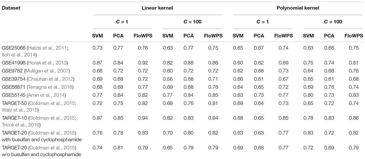
Table 3. AUC of (non)responder classifier for classical SVM without data reduction (SVM), PCA-assisted SVM (PCA) and FloWPS with confidence parameter p = 0.90.
Discussion
It was seen previously that SVM sometimes fails when it is intended for distinguishing fine biomedical properties such as disease progression prognosis or assessment of clinical efficiency of drugs for an individual patient, using high throughput molecular data, e.g., complete DNA mutation or gene expression profiles (Ray and Zhang, 2009; Babaoglu et al., 2010). Particularly, for many biologically relevant applications, SVM occurred either fully incapable to predict drug sensitivity (Turki and Wei, 2016), or demonstrated poorer performance than competing method for machine learning (Davoudi et al., 2017; Cho et al., 2018; Jeong et al., 2018; Leite et al., 2018; Sauer et al., 2018; Yosipof et al., 2018). Thus, the tool for improvement of SVM performance is certainly needed.
In this study, we investigated ten sets of gene expression data for cancer patients treated with different anti-cancer drugs with known clinical outcomes, where the original dimension of samples (patients) is many hundreds times larger than the numbers of patients. So, the first problem in such applications was to extract an appropriate number of features, in which space one could achieve a classifier-predictor with a high level of quality. There are many authors focused to resolve the preprocessing problem (Tan and Gilbert, 2003; Kourou et al., 2015; Tan, 2016; Liu et al., 2017; Tarek et al., 2017). Some feature selection methods, like the DWFS wrapping tool (Soufan et al., 2015), use sophisticatedly designed approaches such as genetic algorithms to improve the classifier quality. In this paper we proposed one more, FloWPS, which is very different from all known. Its critical characteristic is that for every single new sample, which class has to be predicted, the method extracted its individual sub-space and, more, in that subspace takes for training data an appropriate subset of samples.
FloWPS data trimming method simultaneously combines the advantages of both global (like SVM) and local (like kNN) (Altman, 1992) methods of machine learning, and successfully acts even when purely local and global approaches fail. The failure of SVM, which we have observed at least for 3 out of 10 datasets in the current study (Table 2), means that there is no strict distant order in the placement of responder and non-responder points in the space of gene expression features. Yet, the lack of distant order does not necessary mean the absence of local order (Figure 6). The latter may be detected using local methods such as kNN, which has been confirmed by our FloWPS (Table 2 and Figures 3, 5). The FloWPS advantages are better seen for SVM with polynomial than for linear kernel due to higher risk of overtraining on such models (Figure 5 and Table 3).
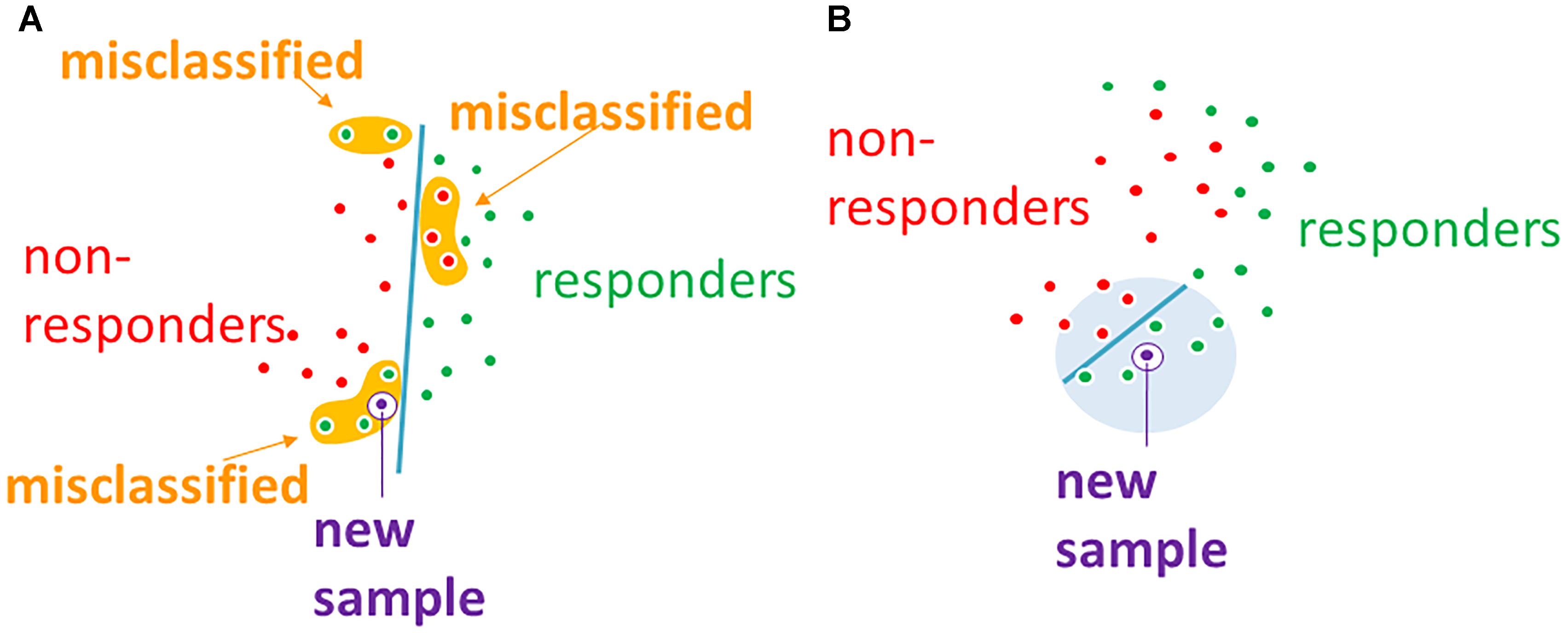
Figure 6. (A) Global machine learning methods, such as SVM, may fail to separate classes in datasets without global order. (B) Machine-learning with data trimming works locally and may separate classes more accurately.
We hypothesize that FloWPS and data trimming may be also helpful for improving other learning methods based on multi-omics data, including nowadays-flourishing deep learning approaches (Bengio et al., 2013; LeCun et al., 2015; Schmidhuber, 2015).
Materials and Methods
Preprocessing of Gene Expression Data
For the datasets investigated using the Affymetrix microarray hybridization platforms, gene expression data were taken from the series matrices deposited in the GEO public repository and then quantile-normalized (Bolstad et al., 2003) using the R package preprocessCore (Bolstad, 2018). All pediatric datasets taken from the TARGET database (Goldman et al., 2015) contained results of NGS mRNA profiling at Illumina HiSeq 2000 platforms; they were normalized using R package DESeq2 (Love et al., 2014).
SVM Calculations
All the SVM calculations with linear and polynomial kernels were performed using the Python package sklearn (Pedregosa et al., 2012) that employs the C++ library ‘libsvm’ (Chang and Lin, 2011). The penalty parameter C varied from 0.1 to 1000 for different calculations. Other SVM parameters had the default settings for the sklearn package.
Plot Preparations
AUC(m,k) topograms, like Figure 2B, were plotted using mathplotlib Python library (Hunter, 2007). Violin plots for FloWPS predictions (see Figure 3) for responders and non-responders were plotted using the ggplot2 R package (Wilkinson, 2011).
Availability of Data and Materials
The datasets analyzed during the current study are available in the GEO repository,
https://www.ncbi.nlm.nih.gov/geo/query/acc.cgi?acc=GSE25066
https://www.ncbi.nlm.nih.gov/geo/query/acc.cgi?acc=GSE41998
https://www.ncbi.nlm.nih.gov/geo/query/acc.cgi?acc=GSE9782
https://www.ncbi.nlm.nih.gov/geo/query/acc.cgi?acc=GSE39754
https://www.ncbi.nlm.nih.gov/geo/query/acc.cgi?acc=GSE68871
https://www.ncbi.nlm.nih.gov/geo/query/acc.cgi?acc=GSE55145
ftp://caftpd.nci.nih.gov/pub/OCG-DCC/TARGET/WT/mRNA-seq/
ftp://caftpd.nci.nih.gov/pub/OCG-DCC/TARGET/AML/mRNA-seq/
ftp://caftpd.nci.nih.gov/pub/OCG-DCC/TARGET/ALL/mRNA-seq/
The Python module that performs data trimming according to the FloWPS method for different values of parameters m and k, as well as the R code that makes FloWPS predictions using the results obtained with the Python module, and a README manual how to use these codes, were deposited on Gitlab and are available by the link: https://gitlab.com/oncobox/flowps.
Ethics Statement
Current research did not involve any new human material. All the gene expression data that were used for research, were taken from publicly available repositories Gene Expression Omnibus (GEO) and TARGET, and had been previously anonymized by the teams, who had worked with them.
Author Contributions
NB designed the overall research, suggested the principles of data trimming and prediction-accountable set, and wrote most parts of the manuscript. VT performed most part of calculations. MS suggested datasets with clinical responders and non-responders and performed feature selection. AM wrote the initial version of computational code. AS adapted this code for parallel calculations. AG tested and debugged the computational code. IM and AB essentially improved the manuscript upon the draft version has been prepared. AB preformed the overall scientific supervision of the project.
Funding
This work was supported by Amazon and Microsoft Azure grants for cloud-based computational facilities. We thank Oncobox/OmicsWay research program in machine learning and digital oncology for software and pathway databases for this study. Financial support was provided by the Russian Science Foundation grant no. 18-15-00061.
Conflict of Interest Statement
VT, MS, AS, AG, AB, and NB were employed by OmicsWay Corporation, Walnut, CA, United States. AM was employed by Yandex N.V. Corporation, Moscow, Russia.
The remaining author declares that the research was conducted in the absence of any commercial or financial relationships that could be construed as a potential conflict of interest.
Supplementary Material
The Supplementary Material for this article can be found online at: https://www.frontiersin.org/articles/10.3389/fgene.2018.00717/full#supplementary-material
Abbreviations
ALL, acute lymphoblastic leukemia; AML, acute myelogenous leukemia; ASCT, allogeneic stem cell transplantation; AUC, area under curve; FDR, false discovery rate; FloWPS, floating window projective separator; FP, false positive; FN, false negative; GEO, gene expression omnibus; GSE, GEO series; HER2, human epidermal growth factor receptor 2; kNN, k nearest neighbors; MCC, Matthews correlation coefficient; mRNA, messenger ribonucleic acid; NGS, next-generation sequencing; PC, principal component; PCA, principal component analysis; ROC, receiver operating characteristic; SVM, support vector machine; TN, true negative; TP, true positive; VTD, velcade, thalidomide and dexamethasone.
Footnotes
- ^This is the result of a PubMed query https://www.ncbi.nlm.nih.gov/pubmed/?term=support+vector+machine_
- ^The ROC (receiver–operator curve) is a widely-used graphical plot that illustrates the diagnostic ability of a binary classifier system as its discrimination threshold is varied. The ROC is created by plotting the true positive rate (TPR) against the false positive rate (FPR) at various threshold settings. The area under the ROC curve, called ROC AUC, or simply AUC, is routinely employed for assessment of any classifier’s quality.
- ^Data trimming is the process of removing or excluding extreme values, or outliers, from a dataset (Turkiewicz, 2017).
- ^FDR shows the percentage of false positive (FP) predictions among all those classified as positive, FDR = FP/(FP + TP), where TP means true positive.
- ^MCC can be calculated from the confusion matrix,
References
Ahmed, F., Ansari, H. R., and Raghava, G. P. S. (2009a). Prediction of guide strand of microRNAs from its sequence and secondary structure. BMC Bioinformatics 10:105. doi: 10.1186/1471-2105-10-105
Ahmed, F., Kumar, M., and Raghava, G. P. S. (2009b). Prediction of polyadenylation signals in human DNA sequences using nucleotide frequencies. In Silico Biol. 9, 135–148.
Ahmed, F., Kaundal, R., and Raghava, G. P. S. (2013). PHDcleav: a SVM based method for predicting human Dicer cleavage sites using sequence and secondary structure of miRNA precursors. BMC Bioinformatics 14(Suppl. 14):S9. doi: 10.1186/1471-2105-14-S14-S9
Altman, N. S. (1992). An introduction to kernel and nearest-neighbor nonparametric regression. Am. Stat. 46, 175–185. doi: 10.1080/00031305.1992.10475879
Amin, S. B., Yip, W.-K., Minvielle, S., Broyl, A., Li, Y., Hanlon, B., et al. (2014). Gene expression profile alone is inadequate in predicting complete response in multiple myeloma. Leukemia 28, 2229–2234. doi: 10.1038/leu.2014.140
Ansari, H. R., and Raghava, G. P. (2010). Identification of conformational B-cell epitopes in an antigen from its primary sequence. Immunome Res. 6:6. doi: 10.1186/1745-7580-6-6
Arimoto, R., Prasad, M.-A., and Gifford, E. M. (2005). Development of CYP3A4 inhibition models: comparisons of machine-learning techniques and molecular descriptors. J. Biomol. Screen. 10, 197–205. doi: 10.1177/1087057104274091
Babaoglu,İ., Findik, O., and Ülker, E. (2010). A comparison of feature selection models utilizing binary particle swarm optimization and genetic algorithm in determining coronary artery disease using support vector machine. Expert Syst. Appl. 37, 3177–3183. doi: 10.1016/j.eswa.2009.09.064
Balabin, R. M., and Lomakina, E. I. (2011). Support vector machine regression (LS-SVM)—an alternative to artificial neural networks (ANNs) for the analysis of quantum chemistry data? Phys. Chem. Chem. Phys. 13, 11710–11718. doi: 10.1039/c1cp00051a
Balabin, R. M., and Smirnov, S. V. (2012). Interpolation and extrapolation problems of multivariate regression in analytical chemistry: benchmarking the robustness on near-infrared (NIR) spectroscopy data. Analyst 137, 1604–1610. doi: 10.1039/c2an15972d
Bengio, Y., Courville, A., and Vincent, P. (2013). Representation learning: a review and new perspectives. IEEE Trans. Pattern Anal. Mach. Intell. 35, 1798–1828. doi: 10.1109/TPAMI.2013.50
Betrie, G. D., Tesfamariam, S., Morin, K. A., and Sadiq, R. (2013). Predicting copper concentrations in acid mine drainage: a comparative analysis of five machine learning techniques. Environ. Monit. Assess. 185, 4171–4182. doi: 10.1007/s10661-012-2859-7
Bolstad, B. (2018). preprocessCore: A Collection of Pre-Processing Functions. R package. Available at: https://github.com/bmbolstad/preprocessCore
Bolstad, B. M., Irizarry, R. A., Astrand, M., and Speed, T. P. (2003). A comparison of normalization methods for high density oligonucleotide array data based on variance and bias. Bioinformatics 19, 185–193. doi: 10.1093/bioinformatics/19.2.185
Chang, C.-C., and Lin, C.-J. (2011). LIBSVM: a library for support vector machines. ACM Trans. Intell. Syst. Technol. 2, 1–27. doi: 10.1145/1961189.1961199
Chauhan, D., Tian, Z., Nicholson, B., Kumar, K. G. S., Zhou, B., Carrasco, R., et al. (2012). A small molecule inhibitor of ubiquitin-specific protease-7 induces apoptosis in multiple myeloma cells and overcomes bortezomib resistance. Cancer Cell 22, 345–358. doi: 10.1016/j.ccr.2012.08.007
Cho, H.-J., Lee, S., Ji, Y. G., and Lee, D. H. (2018). Association of specific gene mutations derived from machine learning with survival in lung adenocarcinoma. PLoS One 13:e0207204. doi: 10.1371/journal.pone.0207204
Davoudi, A., Ozrazgat-Baslanti, T., Ebadi, A., Bursian, A. C., Bihorac, A., and Rashidi, P. (2017). “Delirium prediction using machine learning models on predictive electronic health records data,” in Proceedings of the 2017 IEEE 17th International Conference on Bioinformatics and Bioengineering (BIBE) (Washington, DC: IEEE), 568–573. doi: 10.1109/BIBE.2017.00014
Goldman, M., Craft, B., Swatloski, T., Cline, M., Morozova, O., Diekhans, M., et al. (2015). The UCSC cancer genomics browser: update 2015. Nucleic Acids Res. 43, D812–D817. doi: 10.1093/nar/gku1073
Hatzis, C., Pusztai, L., Valero, V., Booser, D. J., Esserman, L., Lluch, A., et al. (2011). A genomic predictor of response and survival following taxane-anthracycline chemotherapy for invasive breast cancer. JAMA 305, 1873–1881. doi: 10.1001/jama.2011.593
Horak, C. E., Pusztai, L., Xing, G., Trifan, O. C., Saura, C., Tseng, L.-M., et al. (2013). Biomarker analysis of neoadjuvant doxorubicin/cyclophosphamide followed by ixabepilone or Paclitaxel in early-stage breast cancer. Clin. Cancer Res. Off. J. Am. Assoc. Cancer Res. 19, 1587–1595. doi: 10.1158/1078-0432.CCR-121359
Hunter, J. D. (2007). Matplotlib: a 2D graphics environment. Comput. Sci. Eng. 9, 90–95. doi: 10.1109/MCSE.2007.55
Itoh, M., Iwamoto, T., Matsuoka, J., Nogami, T., Motoki, T., Shien, T., et al. (2014). Estrogen receptor (ER) mRNA expression and molecular subtype distribution in ER-negative/progesterone receptor-positive breast cancers. Breast Cancer Res. Treat. 143, 403–409. doi: 10.1007/s10549-013-2763-z
Jeong, E., Park, N., Choi, Y., Park, R. W., and Yoon, D. (2018). Machine learning model combining features from algorithms with different analytical methodologies to detect laboratory-event-related adverse drug reaction signals. PLoS One 13:e0207749. doi: 10.1371/journal.pone.0207749
Kim, Y. R., Kim, D., and Kim, S. Y. (2018). Prediction of acquired taxane resistance using a personalized pathway-based machine learning method. Cancer Res. Treat. doi: 10.4143/crt.2018.137 [Epub ahead of print].
Kourou, K., Exarchos, T. P., Exarchos, K. P., Karamouzis, M. V., and Fotiadis, D. I. (2015). Machine learning applications in cancer prognosis and prediction. Comput. Struct. Biotechnol. J. 13, 8–17. doi: 10.1016/j.csbj.2014.11.005
LeCun, Y., Bengio, Y., and Hinton, G. (2015). Deep learning. Nature 521, 436–444. doi: 10.1038/nature14539
Leite, D. M. C., Brochet, X., Resch, G., Que, Y.-A., Neves, A., and Peña-Reyes, C. (2018). Computational prediction of inter-species relationships through omics data analysis and machine learning. BMC Bioinformatics 19:420. doi: 10.1186/s12859-018-2388-7
Liu, J., Wang, X., Cheng, Y., and Zhang, L. (2017). Tumor gene expression data classification via sample expansion-based deep learning. Oncotarget 8, 109646–109660. doi: 10.18632/oncotarget.22762
Love, M. I., Huber, W., and Anders, S. (2014). Moderated estimation of fold change and dispersion for RNA-seq data with DESeq2. Genome Biol. 15:550. doi: 10.1186/s13059-014-0550-8
Mamoshina, P., Volosnikova, M., Ozerov, I. V., Putin, E., Skibina, E., Cortese, F., et al. (2018). Machine learning on human muscle transcriptomic data for biomarker discovery and tissue-specific drug target identification. Front. Genet. 9:242. doi: 10.3389/fgene.2018.00242
Mulligan, G., Mitsiades, C., Bryant, B., Zhan, F., Chng, W. J., Roels, S., et al. (2007). Gene expression profiling and correlation with outcome in clinical trials of the proteasome inhibitor bortezomib. Blood 109, 3177–3188. doi: 10.1182/blood-2006-09-044974
Pedregosa, F., Varoquaux, G., Gramfort, A., Michel, V., Thirion, B., Grisel, O., et al. (2012). Scikit-learn: machine learning in python. arXiv [Preprint]. arXiv:1201.0490
Ray, M., and Zhang, W. (2009). Integrating gene expression and phenotypic information to analyze Alzheimer’s disease. J. Alzheimers Dis. 16, 73–84. doi: 10.3233/JAD-2009-0917
Sauer, C. M., Sasson, D., Paik, K. E., McCague, N., Celi, L. A., Sánchez Fernández, I., et al. (2018). Feature selection and prediction of treatment failure in tuberculosis. PLoS One 13:e0207491. doi: 10.1371/journal.pone.0207491
Schmidhuber, J. (2015). Deep learning in neural networks: an overview. Neural Netw. Off. J. Int. Neural Netw. Soc. 61, 85–117. doi: 10.1016/j.neunet.2014.09.003
Soufan, O., Kleftogiannis, D., Kalnis, P., and Bajic, V. B. (2015). DWFS:a wrapper feature selection tool based on a parallel genetic algorithm. PLoS One 10:e0117988. doi: 10.1371/journal.pone.0117988
Tan, A. C., and Gilbert, D. (2003). Ensemble machine learning on gene expression data for cancer classification. Appl. Bioinformatics 2, S75–S83.
Tan, M. (2016). Prediction of anti-cancer drug response by kernelized multi-task learning. Artif. Intell. Med. 73, 70–77. doi: 10.1016/j.artmed.2016.09.004
Tarek, S., Abd Elwahab, R., and Shoman, M. (2017). Gene expression based cancer classification. Egpt. Inform. J. 18, 151–159. doi: 10.1016/j.eij.2016.12.001
Terragna, C., Remondini, D., Martello, M., Zamagni, E., Pantani, L., Patriarca, F., et al. (2016). The genetic and genomic background of multiple myeloma patients achieving complete response after induction therapy with bortezomib, thalidomide and dexamethasone (VTD). Oncotarget 7, 9666–9679. doi: 10.18632/oncotarget.5718
Tricoli, J. V., Blair, D. G., Anders, C. K., Bleyer, W. A., Boardman, L. A., Khan, J., et al. (2016). Biologic and clinical characteristics of adolescent and young adult cancers: acute lymphoblastic leukemia, colorectal cancer, breast cancer, melanoma, and sarcoma: biology of AYA Cancers. Cancer 122, 1017–1028. doi: 10.1002/cncr.29871
Turki, T., and Wei, Z. (2016). “Learning approaches to improve prediction of drug sensitivity in breast cancer patients,” in Proceedings of the 2016 38th Annual International Conference of the IEEE Engineering in Medicine and Biology Society (EMBC) (Orlando, FL: IEEE), 3314–3320. doi: 10.1109/EMBC.2016.7591437
Turkiewicz, K. L. (2017). The SAGE Encyclopedia of Communication Research Methods. Thousand Oaks, CA: SAGE Publications, Inc. doi: 10.4135/9781483381411.n130
Walz, A. L., Ooms, A., Gadd, S., Gerhard, D. S., Smith, M. A., Guidry Auvil, J. M., et al. (2015). Recurrent DGCR8, DROSHA, and SIX homeodomain mutations in favorable histology wilms tumors. Cancer Cell 27, 286–297. doi: 10.1016/j.ccell.2015.01.003
Wilkinson, L. (2011). ggplot2: elegant graphics for data analysis by WICKHAM, H. Biometrics 67, 678–679. doi: 10.1111/j.1541-0420.2011.01616.x
Yosipof, A., Guedes, R. C., and García-Sosa, A. T. (2018). Data mining and machine learning models for predicting drug likeness and their disease or organ category. Front. Chem. 6:162. doi: 10.3389/fchem.2018.00162
Keywords: bioinformatics, machine learning, oncology, gene expression, support vector machines, personalized medicine
Citation: Tkachev V, Sorokin M, Mescheryakov A, Simonov A, Garazha A, Buzdin A, Muchnik I and Borisov N (2019) FLOating-Window Projective Separator (FloWPS): A Data Trimming Tool for Support Vector Machines (SVM) to Improve Robustness of the Classifier. Front. Genet. 9:717. doi: 10.3389/fgene.2018.00717
Received: 01 September 2018; Accepted: 21 December 2018;
Published: 15 January 2019.
Edited by:
Tao Huang, Shanghai Institutes for Biological Sciences (CAS), ChinaReviewed by:
Guilherme De Alencar Barreto, Universidade Federal do Ceará, BrazilFiroz Ahmed, Jeddah University, Saudi Arabia
Copyright © 2019 Tkachev, Sorokin, Mescheryakov, Simonov, Garazha, Buzdin, Muchnik and Borisov. This is an open-access article distributed under the terms of the Creative Commons Attribution License (CC BY). The use, distribution or reproduction in other forums is permitted, provided the original author(s) and the copyright owner(s) are credited and that the original publication in this journal is cited, in accordance with accepted academic practice. No use, distribution or reproduction is permitted which does not comply with these terms.
*Correspondence: Nicolas Borisov, Ym9yaXNvdkBvbmNvYm94LmNvbQ==