Estimation of Heterogeneous Restricted Mean Survival Time Using Random Forest

Estimation and prediction of heterogeneous restricted mean survival time (hRMST) is of great clinical importance, which can provide an easily interpretable and clinically meaningful summary of the survival function in the presence of censoring and individual covariates. The existing methods for the modeling of hRMST rely on proportional hazards or other parametric assumptions on the survival distribution. In this paper, we propose a random forest based estimation of hRMST for right-censored survival data with covariates and prove a central limit theorem for the resulting estimator. In addition, we present a computationally efficient construction for the confidence interval of hRMST. Our simulations show that the resulting confidence intervals have the correct coverage probability of the hRMST, and the random forest based estimate of hRMST has smaller prediction errors than the parametric models when the models are mis-specified. We apply the method to the ovarian cancer data set from The Cancer Genome Atlas (TCGA) project to predict hRMST and show an improved prediction performance over the existing methods. A software implementation, srf using R and C++, is available at https://github.com/lmy1019/SRF.

1. Introduction

In epidemiological and biomedical studies, time to an event or survival time T is often the primary outcome of interest. Important quantities related to survival time include hazard rate (HR), t-year survival probability, and the mean survival time. Among these, HR is one of the most commonly used quantity due to its strong connection to the proportional hazards regression model or Cox model. Cox model is a very popular regression model for censored survival data due to its computational feasibility and theoretical properties (Cox, 1972, 1975; Andersen and Gill, 1982; Gill and Gill, 1984; Huang et al., 2013; Fang et al., 2017). However, when there is a departure from the proportional hazards assumption, the connection between HR and survival function is lost and it is difficult to interpret HR (Wang and Schaubel, 2018). The t-year survival probability is the probability of survival time greater than a pre-specified time t. It is not suitable for summarizing the global profile of T over the duration of a study (Tian et al., 2014). In contrast, mean survival time is an alternative quantity since it takes the whole distribution of T into account. However, the mean of T may not always be estimable in the presence of censoring. For example, let C denotes the censoring time, and $C_{max}={inf}_c\left\{P(C\le c)=1\right\}$ be the upper limit of the censoring distribution,

$\begin{array}{l}{E}_T\left[T\right]=E_T\left[T|T\le C_{max}\right]P(T\le C_{max})\\ +E_T\left[T|T>C_{max}\right]P(T>C_{max})\end{array}$

If the survival time T satisfies P(T > C_max) > 0, then we cannot estimate E_T[T], since we never observe any event after C_max.

The restricted mean survival time (RMST) (Royston and Parmar, 2013) summarizes the survival process and provides an attractive alternative to the proportional hazards regression model (Tian et al., 2014). The restricted survival time of T up to a fixed point L is defined as T ∧ L, and the restricted mean survival time is defined as the expectation of the restricted survival time. Denote μ^L(x) = E[T ∧ L|X = x] be the heterogeneous RMST with covariates X = x. It can be written as the area under the survival curve on [0, L].

$\begin{array}{ll}\begin{array}{l}{\mu }^L(x)={\displaystyle {\int }_0^{\infty }}\left({\displaystyle {\int }_0^{\infty }}{1}_{u<t}{1}_{u<L}du\right)f_T(t|X=x)dt\\ ={\displaystyle {\int }_0^L}S(u|X=x)du.\end{array}& (1)\end{array}$

If L is chosen to be less than C_max, hRMST is estimable since P(T ∧ L > C_max) = 0. RMST also plays a role in the context of inverse probability censoring weighting (IPCW). A key assumption for applying IPCW is P(T < C_max) = 1, making 1/(1 − G(T)) well-defined, where G(T) = P(C ≤ T|T). If we set L properly such that P(T ∧ L < C_max) = 1, then G(T ∧ C ∧ L|X) < 1 and the IPCW is well-defined under the restricted survival time context.

There are two main approaches for hRMST regression. One approach is to estimate hRMST indirectly through hazard regression (Zucker, 1998; Chen and Tsiatis, 2001; Zhang and Schaubel, 2011). This approach starts by estimating the regression parameters and the baseline hazard from a Cox model, calculating the cumulative baseline hazard, transforming it to obtain the survival function and, finally, obtaining the hRMST through Equation (1). Such an indirect hRMST estimation is inconvenient and computationally cumbersome for obtaining a point estimate and its corresponding asymptotic standard error. An alternative approach is to model hRMST with the baseline covariates X directly via some parametric assumptions, eg. $g\left[{\mu }^L(X_i)\right]={\beta }_0^{\prime }{X}_i,$ where g is a strictly monotone link function with a continuous derivative within an open neighborhood (Tian et al., 2014; Wang and Schaubel, 2018). A major weakness of this approach, however, is their inability to choose a proper link function, which may lead to the model misspecification. As an example, we simulate x₁, …, x_n independently from the uniform distribution on [0, 1]²⁰ with a survival time model

$\begin{array}{ll}T=exp(2X_1+5)+1+ϵ,ϵ~N(0,10^2),& (2)\end{array}$

where we assume that the censoring time C and the restricted time L satisfy P(C ≤ T ∧ L) = 33% and P(L ≤ T ∧ C) = 11%. Our goal is to estimate μ^L(x). Figure 1 shows a set of predictions on an artificially generated data set from Equation (2). Compared with other methods, the random forest is able to estimate the target function closely, especially when μ^L(x) approaches L.

FIGURE 1

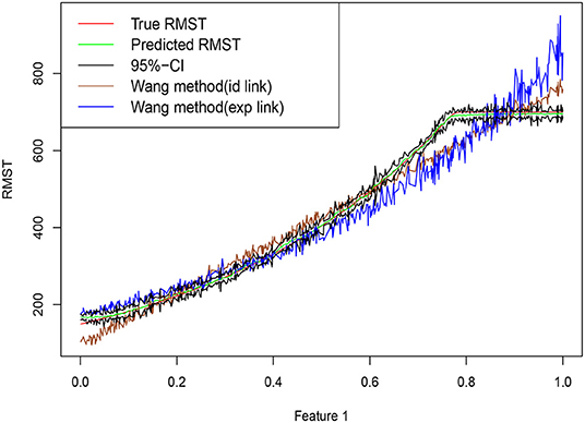
Figure 1. Training data are simulated from Equation (2), with n = 600 training points, dimension p = 20 and errors ϵ ~ N(0, 10²). Random forests are trained based using R package grf. Truth is shown as red curve, with green curve corresponding to the random forest predictions, and upper and lower bounds of the point-wise confidence intervals connected in the black lines. Brown curve and blue curve are based on the approaches of Wang and Schaubel (2018) with Identity and Exp link functions.

For the continuous outcomes without censoring, random forest (Breiman, 2001, 2004) is a popular method of non-parametric regression that has shown effectiveness in many applications (Svetnik et al., 2003; Díaz-Uriarte and Alvarez de Andrés, 2006; Cutler et al., 2007). It is invariant under scaling and various other transformations of feature values, robust to inclusion of irrelevant features (Hastie et al., 2001), and versatile enough to be applied to large-scale problems (Biau and Scornet, 2016). Besides strong empirical results, theoretical results such as consistency (Meinshausen, 2006; Biau et al., 2008; Biau, 2012; Denil et al., 2014) and asymptotic normality (Wager and Athey, 2015; Mentch and Hooker, 2016; Athey et al., 2018; Friedberg et al., 2018) have also been obtained for regression models without censoring. Extending random forest to censored survival data has been proposed in several recent papers (Ishwaran et al., 2008; Steingrimsson et al., 2019), focusing on implementations and algorithms. However, there has been little theoretical work in statistical inference of such random survival forest. Ishwaran and Kogalur (2011) proved the consistency of the random survival forest by showing that the forest ensemble survival function converges uniformly to the true population survival function.

Instead of focusing on predicting the survival function or the survival probability as the algorithms implemented by Ishwaran et al. (2008) and Steingrimsson et al. (2019), we develop in this paper a random forest framework to model the hRMST directly given the baseline covariates in the presence of possibly covariate-dependent censoring. This approach provides a non-parametric estimation of hRMST adjusting for covariates. Due to the complex relationship between the survival time and the covariates, it is desirable to have more flexible methods to estimate the hRMST than the approaches that a certain link function has to be assumed. Our construction of random forest is based on the estimated IPCW. We show that the resulting survival random forest estimates of hRMST has the asymptotic normality property that can be used to obtain the point-wise confidence interval with theoretical guarantees. To the best of our knowledge, it is the first asymptotic normality result for the predictions in the context of censored survival data using random forest.

The remainder of the paper is organized as follows. In section 2, we describe the proposed random forest estimator. Asymptotic properties are given in section 3. In section 4, we conduct simulation studies to evaluate the accuracy of the proposed method in the finite sample settings. In section 5, we apply our method to an ovarian cancer data set of The Cancer Genome Atlas (TCGA) project (http://cancergenome.nih.gov/abouttcga) to evaluate the predictions of the hRMST for ovarian cancer patients using their acylcarnitine measurements and clinical variables. We conclude this chapter with a brief discussion in section 6.

2. Random Forest for Estimating the hRMST

We begin with some notation. Let X_i be the baseline covariates for subject i from a cohort of sample size n and T_i be the survival time for subject i. Let C_i be the censoring time, which is independent of T_i conditional on the baseline covariates X_i. The observation time for subject i is Z_i = T_i ∧ C_i, where a ∧ b = min{a, b}. The indicator for censoring is denoted by δ_i = 1_{{Ti ≤ Ci}}. Our observed i.i.d. data are given as {(X_i, Z_i, δ_i):i = 1, …, n}.

Let L be a pre-specified time point of interest, before the maximum follow-up time τ = max{Z_i : i = 1, …, n}. As in Wang and Schaubel (2018), L is normally chosen as a time point of clinical relevance or, at least, of particular interest to the investigators, respecting the bound at the maximum follow-up time. Denote the restricted observation time as $Z_i^L=Z_i\wedge L$ and its corresponding indicator ${\delta }_i^L=1_{\left\{T_i\wedge L\le C_i\right\}}$. Our goal is to estimate covariate-adjusted RMST or hRMST μ^L(x) = E(Z^L|X = x) and to construct its confidence interval.

2.1. Forest-Based Local Estimating Equation for hRMST

Given the observed data ${\left\{(X_i,{\delta }_i,Z_i)\right\}}_{i=1}^n$, and a restriction threshold L, we first present a random forest method to estimate μ^L(x). The idea of the approach is to solve a weighted estimating equation for μ^L(x), where the estimating equation functions of the observations whose covariates closer to x will have larger weights. Specifically, let $w_i={\delta }_i^L/(1-G(Z_i^L|X_i))$ be the IPCW of the ith data point under the true censoring distribution G(·|X_i). The (infeasible) estimating equation function $w_i(Z_i^L-{\mu }^L(x))$ of X_i = x satisfies $E\left[w_i(Z_i^L-{\mu }^L(x))|X_i=x\right]=E\left[T_i\wedge L|X_i=x\right]-{\mu }^L(x)=0$. If the local weights ${\left\{{\alpha }_i(x)\right\}}_{i=1}^n$ are also known, the solution to the empirical estimating equation for μ^L(x)

$\begin{array}{ll}\begin{array}{c}{\displaystyle \sum _{i=1}^n}{\alpha }_i(x)w_i(Z_i^L-\mu )=0\end{array}& (3)\end{array}$

is given as

$\frac{{\displaystyle {\sum }_{i=1}^n}{\alpha }_i(x)w_i{Z}_i^L}{{\displaystyle {\sum }_{i=1}^n}{\alpha }_i(x)w_i},$

which provides a good candidate of estimator for μ^L(x). However we do not know the censoring distribution G and the local weights ${\left\{{\alpha }_i(x)\right\}}_{i=1}^n$, which need to be estimated from the data. We assume censoring distribution G follows a Cox model, a natural choice for modeling censoring times in the context of IPCW. Let

${\widehat{w}}_i=\frac{{\delta }_i^L}{1-\widehat{G}(Z_i^L|X_i)}$

be the estimated IPCW for ith observation with Ĝ(·|X_i) derived from the data through Cox model. We define the estimating equation function for ith observation with its corresponding estimated IPCW as

${\psi }_{{\mu }^L(x)}(X_i,Z_i^L,{\delta }_i^L)={\widehat{w}}_i(Z_i^L-{\mu }_i^L(x)).$

Our approach to derive the local weights ${\left\{{\alpha }_i(x)\right\}}_{i=1}^n$ is through the random forest, which is an ensemble of survival trees constructed by Algorithm 1.

ALGORITHM 1

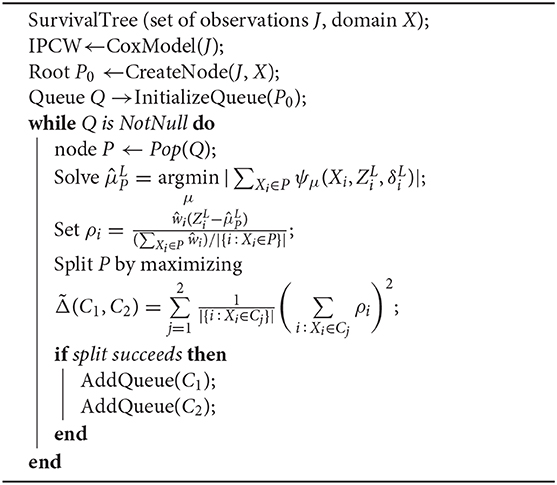
Algorithm 1: Survival tree

It can be shown that ρ_i is the influence function of the ith observation for ${\widehat{\mu }}_P^L$. Let F_n be the empirical distribution of the observations in node P, and let F_n,i = (1 − ϵ)F_n + ϵ ν_i, with ν_i be the Dirac delta function at ith observation. Set ${\widehat{\mu }}_{P,i}^L={\widehat{\mu }}_P^L+{\Delta }_i$, where ${\widehat{\mu }}_{P,i}^L=\begin{array}{c}argmin\\ \mu \end{array}|\int {\psi }_{\mu }(X,Z^L,{\delta }^L)d{F}_{n,i}|$. By Taylor expansion,

$\begin{array}{l}0={\displaystyle \int }{\psi }_{{\widehat{\mu }}_{P,i}^L}(X,Z^L,{\delta }^L)d{F}_{n,i}\\ ={\displaystyle \int }[{\psi }_{{\widehat{\mu }}_P^L}(X,Z^L,{\delta }^L)+{\psi }_{{\mu }^{*}}^{\prime }(X,Z^L,{\delta }^L){\Delta }_i]d{F}_{n,i},\end{array}$

where μ^* is a value between ${\widehat{\mu }}_P^L$ and ${\widehat{\mu }}_{P,i}^L$. The above equation implies

${\Delta }_i=-\frac{ϵ{\psi }_{{\widehat{\mu }}_P^L}(X_i,Z_i^L,{\delta }_i^L)}{\int {\psi }_{{\mu }^{*}}^{\prime }(X,Z^L,{\delta }^L)d{F}_{n,i}},$

and therefore the influence function of ith observation for ${\widehat{\mu }}_P^L$ is

${\displaystyle \underset{ϵ\to 0}{lim}}{\Delta }_i/ϵ=-\frac{{\psi }_{{\widehat{\mu }}_P^L}(X_i,Z_i^L,{\delta }_i^L)}{\int {\psi }_{{\widehat{\mu }}_P^L}^{\prime }(X,Z^L,{\delta }^L)d{F}_n}=\frac{{\widehat{w}}_i(Z_i^L-{\widehat{\mu }}_P^L)}{{\displaystyle {\sum }_{i\in P}}\frac{{\widehat{w}}_i}{|\{i:X_i\in P\}|}}={\rho }_i.$

Athey et al. (2018) shows that maximizing the splitting criterion $\tilde{\Delta }(C_1,C_2)$ is approximately equivalent to minimizing the weighted mean squared error $err(C_1,C_2)=\sum _{i=1,2}P(X\in C_i|X\in P)E[{({\widehat{\mu }}_{C_i}^L-{\mu }^L(X))}^2|X\in C_i]$.

In order to achieve consistency and asymptotic normality, we split the tree and make predictions in an honest way as introduced in Wager and Athey (2015). Specifically, each tree in an honest forest is grown using two non-overlapping subsamples of the training data. For the bth tree, given I_b and J_b, we first choose the tree structure T_b using only the data in J_b, and write $x{\leftrightarrow }_b{x}^{\prime }$ as the boolean indicator for whether the points x and x′ fall into the same leaf of T_b. In a second step, we define the set of neighbors of x as L_b(x) = {i ∈ I_b : x ↔ _bx_i}. The weights of point x from a survival forest with B trees can be written as

${\alpha }_i(x)=\frac{1}{B}{\displaystyle \sum _{b=1}^B}\frac{1_{\left\{X_i\in L_b(x)\right\}}}{|L_b(x)|}.$

The empirical locally weighted estimating equation for ${\widehat{\mu }}^L(x)$ is then defined as

$\begin{array}{ll}{\displaystyle \sum _{i=1}^n}{\alpha }_i(x){\psi }_{\mu }(X_i,Z_i^L,{\delta }_i^L)=0,& (4)\end{array}$

and the random forest estimator for the hRMST is the solution of Equation (4), which is

${\widehat{\mu }}^L(x)={\displaystyle \sum _{i=1}^n}\frac{{\alpha }_i(x){\widehat{w}}_i{Z}_i^L}{{\displaystyle {\sum }_{i=1}^n}{\alpha }_i(x){\widehat{w}}_i}.$

We emphasize the difference between the IPCW used in building the survival trees and IPCW used to derive ${\widehat{\mu }}^L(x)$. The IPCW used in building survival trees is estimated only by the data points from J_b so that the resulting survival forest is honest. The IPCW used to derive ${\widehat{\mu }}^L(x)$ is estimated from all data points.

3. Asymptotic Distribution of ${\widehat{\mu }}^L(x)$

3.1. Asymptotic Normality

We derive a central limit theorem for survival forest estimate of hRMST. We first give three common assumptions that required for the most of the theoretical analysis of random forests.

Assumption 1. μ^L(x) is Lipschitz continuous w.r.t x.

Assumption 2. There exists a restricted time threshold L, such that P(C > t ∧ L|X = x) ≥ ϵ_L > 0 for any x, t.

Assumption 3. Var(T ∧ L|X = x) > 0 for any x.

As mentioned in the previous section, we model the conditional survival function of censoring distribution G given baseline covariates. Because of its flexibility and popularity in practice, we adopt the proportional hazards model for hazard function of censoring distribution.

Assumption 4. The hazard function of censoring distribution follows ${\lambda }_i^C(t)={\lambda }_0^C(t)exp(X_i^{\prime }{\beta }_C)$

We make additional regularity assumptions that are widely used in analysis of estimates from the proportional hazards models. These assumptions are needed in order to quantify the difference between the estimated IPCW and true IPCW.

Assumption 5. ‖X‖_∞ < M_X < ∞

Assumption 6. ${\lambda }_0^C(t)\le {\lambda }_0^C<\infty$ for all t.

Assumption 7. ${\Omega }_C(\beta )=E[{\int }_0^{\tau }\frac{r^{(2)}(t,\beta )}{r^{(0)}(t,\beta )}-\bar{x}{(t,\beta )}^{\otimes 2}d{N}_i^C(t)]$ is positive definite, where R_i(t) = 1(Z_i ≥ t), $r^{(k)}(t,\beta )=E[exp({\beta }^{\prime }{X}_i)R_i(t)X_i^{\otimes k}]$, $\bar{x}(t,\beta )=\frac{r^{(1)}(t,\beta )}{r^{(0)}(t,\beta )},N_i^C(t)=1_{Z_i\le t,{\delta }_i=0}$.

Assumption 8. P(R_i(t) = 1|X_i = x) ≥ r > 0 for some positive constant and for any t, x. This assumption implies that

$r^{(0)}(t,\beta )=E\left[exp({\beta }^{\prime }{X}_i)R_i(t)\right]=E\left[exp({\beta }^{\prime }{X}_i)E\left[R_i(t)|X_i\right]\right]\ge r>0.$

Following Wager and Athey (2015) and Athey et al. (2018), we assume that all trees are symmetric, in that their output is invariant to permuting the indices of Estimation-Part in training examples (see Corollary 6 of Wager and Athey (2015) for more details about this symmetry). They also require balanced splits in the sense that every split puts at least a fraction ω of the observations in the parent node into each child, for some ω > 0. Finally, the trees are randomized in such a way that, at every split, the probability that the tree splits on the jth feature is bounded from below by some π > 0. The forest is honest and built via subsampling with subsample size s satisfying s/n → 0 and s → ∞.

Under the assumptions listed above, we have the following asymptotic distribution result for the random forest-based estimate of the hRMST.

Theorem 1. Under Assumptions 1, 2, 3, 4, 5, 6, 7, 8, for each fixed test point x, there is a sequence ${\sigma }_n^2(x)=Var({\widehat{\mu }}^L(x))\to 0$,

$\frac{{\widehat{\mu }}^L(x)-{\mu }^L(x)}{{\sigma }_n(x)}{\to }_{d}N(0,1)$

if subsampling size

${\beta }_{min}=1-(1+\frac{{\pi }^{-1}(log({\omega }^{-1}))}{log\left({(1-\omega )}^{-1}\right)}{)}^{-1},$

where ω > 0 is the low-bound fraction for observations in the parent node into each child, and π > 0 is the lower-bound of the probability that the tree splits on any features.

We give a consistent estimate of ${\sigma }_n^2(x)$ based on half-sampling (Efron, 1980) and the method of Sexton and Laake (2009).

3.2. Estimation of the Variance

Following Athey et al. (2018), we use the random forest delta method to develop a variance estimate of the survival forest prediction ${\widehat{\mu }}^L(x)$. Athey et al. (2018) provides a consistent estimate of ${\sigma }_n^2(x)$ using $s_n^2(x)$, where $s_n^2(x)=(V{(x)}^{-1})H_n(x){(V{(x)}^{-1})}^{\prime }$ with

$\begin{array}{l}{H}_n(x)=Var[{\displaystyle \sum _{i=1}^n}{\alpha }_i(x){\psi }_{{\mu }^L(x)}(X_i,Z_i^L,{\delta }_i^L)]\\ V(x)=\frac{\partial }{\partial ({\mu }^L)}E[{\psi }_{{\mu }^L}(X,Z^L,{\delta }^L)|X=x]{|}_{{\mu }^L={\mu }^L(x)}\end{array}$

In our context, V(x) = − 1, then simply we have $s_n^2(x)=H_n(x)$.

A consistent estimator for H_n(x) can be obtained using half-sampling estimator (Efron, 1980; Athey et al., 2018). Let ${\text{Ψ}}_{{H}}$ be the average of the empirical estimating equation functions averaged over the trees that only use the data from the half-sample ${H}$, denoted by $S_{{H}}$,

${\text{Ψ}}_{{H}}(x)=\frac{1}{|S_{{H}}|}{\displaystyle \sum _{b\in S_{{H}}}}\frac{{\displaystyle {\sum }_{i=1}^n}{1}_{X_i\in L_b(x)}{\psi }_{{\widehat{\mu }}^L(x)}(X_i,Z_i^L,{\delta }_i^L)}{{\displaystyle {\sum }_{i=1}^n}{1}_{X_i\in L_b(x)}},$

where L_b(x) contains neighbors of x in the bth tree. An ideal half-sampling estimator is then defined as

$\begin{array}{l}{\widehat{H}}_n^{HS}(x)={\left(\begin{array}{c}n\\ n/2\end{array}\right)}^{-1}{\displaystyle \sum _{{H}:|{H}|=n/2}}{(E_{\Theta }\left[{\text{Ψ}}_{{H}}(x)\right]-E_{\Theta }\overline{\text{Ψ}}(x))}^2\\ \overline{\text{Ψ}}(x)={\left(\begin{array}{c}n\\ n/2\end{array}\right)}^{-1}{\displaystyle \sum _{{H}:|{H}|=n/2}}{\text{Ψ}}_{{H}}(x)\end{array}$

where Θ is the randomness in building honest tree, including splitting data into random halves and randomness in selecting variables to split. ${\widehat{H}}_n^{HS}(x)$ is similar to classic bootstrap estimator for the standard error, except that the sampling distribution for ${\widehat{H}}_n^{HS}(x)$ is the half sampling distribution instead of the bootstrap sampling. Denote E_ss and Var_ss as the expectation and variance under the half sampling distribution, then ${\widehat{H}}_n^{HS}(x)=Va{r}_{ss}\left[E_{\Theta }\left[{\text{Ψ}}_{{H}}(x)\right]\right]$.

Since carrying out the full half-sampling computation and expectation with respect to Θ are impractical, Sexton and Laake (2009) pointed out that ${\widehat{H}}_n^{HS}(x)$ can be efficiently approximated by the following law of total variance:

$\begin{array}{l}{\widehat{H}}_n^{HS}(x)=Va{r}_{ss}\left[E_{\Theta }[\frac{1}{M}{\displaystyle \sum _{m=1}^M}{\text{Ψ}}_{{H},{\Theta }_m}(x)]\right]\\ =Va{r}_{ss}\left[\frac{1}{M}{\displaystyle \sum _{m=1}^M}{\text{Ψ}}_{{H},{\Theta }_m}(x)\right]\\ -E_{ss}\left[Va{r}_{\Theta }[\frac{1}{M}{\displaystyle \sum _{m=1}^M}{\text{Ψ}}_{{H},{\Theta }_m}(x)]\right]& (5)\end{array}$

which leads to a Monte Carlo approximation of ${\widehat{H}}_n^{HS}(x)$ by

$\begin{array}{l}{\widehat{\sigma }}_n^2(x)={\widehat{Var}}_{ss}\left[\frac{1}{M}{\displaystyle \sum _{m=1}^M}{\text{Ψ}}_{{H},{\Theta }_m}(x)\right]\\ -{\widehat{E}}_{ss}\left[{\widehat{Var}}_{\Theta }[\frac{1}{M}{\displaystyle \sum _{m=1}^M}{\text{Ψ}}_{{H},{\Theta }_m}(x)]\right].& (6)\end{array}$

In order to approximate random forest randomness quantity ${\widehat{Var}}_{\Theta }$ and sampling randomness quantities ${\widehat{Var}}_{ss},{\widehat{E}}_{ss}$, we split B trees in G groups and each group has l trees, and the trees in the same group have the same half sample. The final consistent estimator ${\widehat{\sigma }}_n^2(x)$ can be written as

$\begin{array}{l}{\widehat{\sigma }}_n^2(x)=\frac{1}{G-1}{\displaystyle \sum _{g=1}^G}{({\overline{\text{Ψ}}}_g(x)-\overline{\text{Ψ}}(x))}^2\\ -\frac{1}{(l-1)}\frac{1}{B}{\displaystyle \sum _{g=1}^G}{\displaystyle \sum _{i=1}^l}{({\text{Ψ}}_{ig}(x)-{\overline{\text{Ψ}}}_g(x))}^2\end{array}$

where ${\overline{\text{Ψ}}}_g(x)=\frac{1}{l}{\displaystyle \sum _{i=1}^l}{\text{Ψ}}_{ig}(x)$, and $\overline{\text{Ψ}}(x)=\frac{1}{G}{\displaystyle \sum _{g=1}^G}{\overline{\text{Ψ}}}_g(x)$.

The following diagram summarizes the procedure of estimating the variance ${\sigma }_n^2(x)$.

$\begin{array}{l}{\sigma }_n^2(x){\displaystyle \underset{}{\overset{\text{Asym.equivalent}}{\leftarrow }}}{s}_n^2(x){\displaystyle \underset{}{\overset{\text{Half-Sampling estimator}}{\leftarrow }}}\\ {\widehat{H}}_n^{HS}(x){\displaystyle \underset{}{\overset{\text{Empirical estimator}}{\leftarrow }}}{\widehat{\sigma }}_n^2(x)\end{array}$

where from left to right, the first arrow is based on Theorem 5 of Athey et al. (2018), the second arrow is based on half-sampling of Efron (1980), and the third arrow is supported by Equations (5) and (6) and the method of Sexton and Laake (2009).

4. Simulation Studies

We present simulations to evaluate the performance of the proposed method in finite sample setting. Two different models for the survival time are considered

• Model 1: $T=g^{-1}({\alpha }_0+\sum _{i=1}^p{\alpha }_i{X}_i)+ϵ$

• Model 2: $T=g^{-1}({\alpha }_0+\sum _{i=1}^p{\alpha }_i{X}_i^2)+ϵ$

where X_i1, …, X_ip are independently generated from Unif(−1, 1), α₀ = 5, α₁ = α₂ = 0.25 and α_i = 0 for i > 2, and ϵ ~ N(0, σ²). The variance σ² is chosen to have proper signal-noise ratio (SNR),

$\text{SNR}=\frac{Var(g^{-1}({\alpha }_0+{\displaystyle {\sum }_{i=1}^p}{\alpha }_i{X}_i))}{Var(ϵ)}.$

We generate the independent censoring time C_i from a Cox model with the following hazard λ = λ_C exp (X₁ log 2) and λ_C is chosen to have a proper un-censoring rate. The link function g can have the following form

• Identity link: g⁻¹(x) = x;

• Exp link: g⁻¹(x) = exp(x);

• Log-exp link: g⁻¹(x) = log(exp(x) + 1).

4.1. Evaluation of Coverage Probability of Predictions

To evaluate the asymptotic results in Theorem 1, we generate five training data sets and one testing data set with the same sample size. The coverage probability performance is evaluated on the testing data set with predictions and confidence intervals derived from 5 independent training data sets. More specifically, for each observation in the testing sample, we obtain the 95% confidence intervals and record how many times a hRMST observation in test sample is within five estimated 95% confidence intervals. The coverage probability of an observation is defined by the its proportion of being covered, and the overall coverage probability of the testing sample is defined by the average of coverage probability of each of its observation. We present the coverage probability results with sample size n = 1, 000, 2, 000, 5, 000 for Model 1, and n = 1, 000, 2, 000, 10, 000 for Model 2. By choosing the proper λ_C, we control the un-censoring rate around 60–70% for different link functions: λ_C ~ 0.08 for Identity link and Log-exp link, and λ_C ~ 0.003 for Exp link. The truncation time L is chosen to make the truncation rate fall into 2%−5%. Specifically, L ~ 5.4 for Identity link and Log-exp link, and L ~ 220 for Exp link.

Figures 2, 3 present the results for Model 1 and Model 2 under three different link functions. We see that the coverage probability approaches to nominal level 95% when the sample size gets larger. If p is smaller, the coverage probability is closer to 95%. This corresponds to the result of Theorem 3 in Wager and Athey (2015), which states that the rate of convergence of the bias of random forest estimator is $O(n^{\frac{K}{p}})$ for some constant K. When the sample size n is fixed, bigger p leads to larger bias in the estimates of hRMST, and under-coverage of the confidence interval. On the other hand, when p is fixed, bigger n results in a smaller bias and leads to a better coverage of the confidence interval.

FIGURE 2

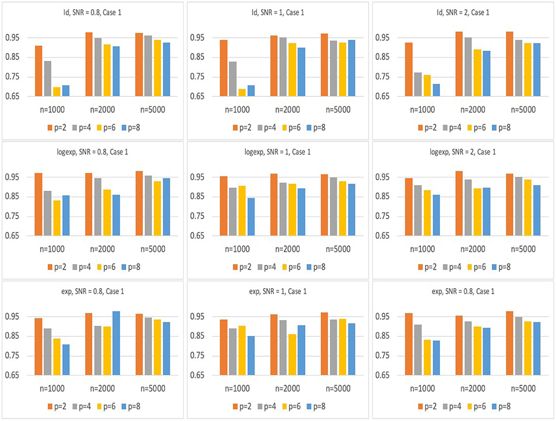
Figure 2. Simulation results of the coverage probability for Model 1 with three different link functions, sample size of n = 1, 000, 2, 000, 5, 000, and p = 2, 4, 6, 8. For each case, prediction coverage probability is calculated over the samples in the testing data set.

FIGURE 3

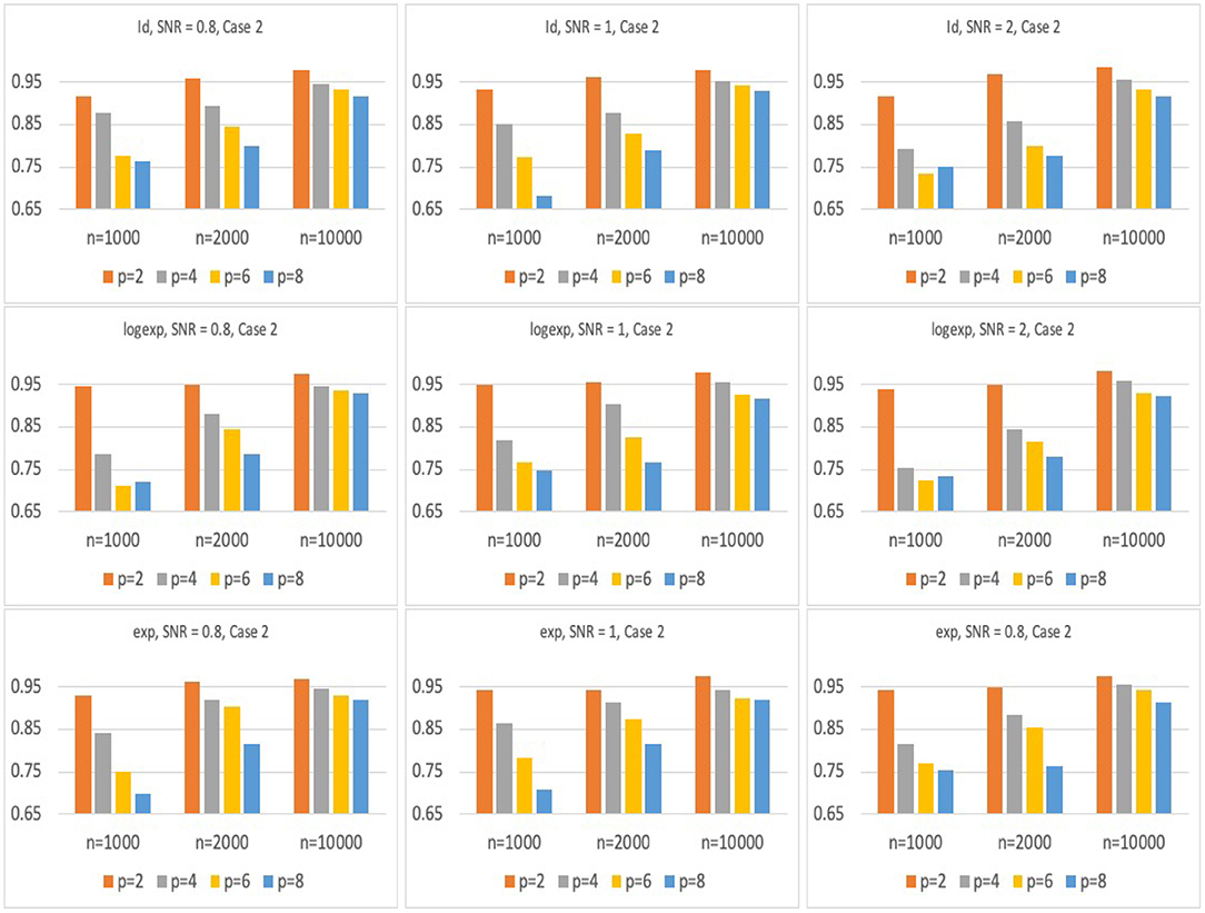
Figure 3. Simulation results of coverage probability for Model 2 with three different link functions, sample size of n = 1, 000, 2, 000, 10, 000, and p = 2, 4, 6, 8. For each case, prediction coverage probability is calculated over the samples in the testing data set.

4.2. Comparison of Prediction Performance With Existing Methods

We compare our proposed method with several existing methods for hRMST estimation, including

• Naive.km: using Kaplan–Meier estimator for survival function and computing hRMST by Equation (1). Covariates are not adjusted.

• Naive.Cox: using proportational hazards estimator for the survival function and computing hRMST by Equation (1). The censoring distribution is assumed to follow the proportional hazards assumption.

• Lu.method: using some parametric forms of hRMST and computing hRMST by solving a weighted estimating equation. The censoring distribution is assumed to be independent of the covariates (Tian et al., 2014). We consider Identity link and Exp link in the simulations.

• Wang.method: using some parametric forms of hRMST and computing hRMST by solving a weighted estimating equation. The censoring distribution is assumed to follow the proportional hazards assumption. We consider Identity link and Exp link in the simulations (Wang and Schaubel, 2018).

We compare all these methods under Model 1 and Model 2, and use the Mean-Absolute-Error (MAE) and Rooted-Mean-Squared-Error (RMSE), introduced in Davison and Hinkley (1997), Tian et al. (2007), and Wang and Schaubel (2018), to measure the performance of these methods.

$\begin{array}{l}\text{MAE}=\frac{1}{n}{\displaystyle \sum _{i=1}^n}\frac{{\delta }_i^L}{1-\widehat{G}(Z_i^L|X_i=x)}|Z_i^L-{\widehat{\mu }}^L(X_i)|,\\ \text{RMSE}=\sqrt{\frac{1}{n}{\displaystyle \sum _{i=1}^n}\frac{{\delta }_i^L}{1-\widehat{G}(Z_i^L|X_i=x)}[Z_i^L-{\widehat{\mu }}^L(X_i){]}^2}.& (7)\end{array}$

We set n = 3, 000, SNR = 0.3. For Identity link and Log-exp link, λ_C = 0.08, L = 5.3. For Exp link λ_C = 0.0026, L = 190. We calculate the MAE and RMSE for our method and four existing methods(both Lu.method and Wang.method have two link functions) under Model 1 and Model 2 and p = 5, 10, 20. Among all the considered models, our method in general has a better performance. As an example, Figure 4 visualizes the observed hRMST generated from Log-exp link and predicted hRMST from our method and Wang.method, showing that the random forest can give better predictions.

FIGURE 4

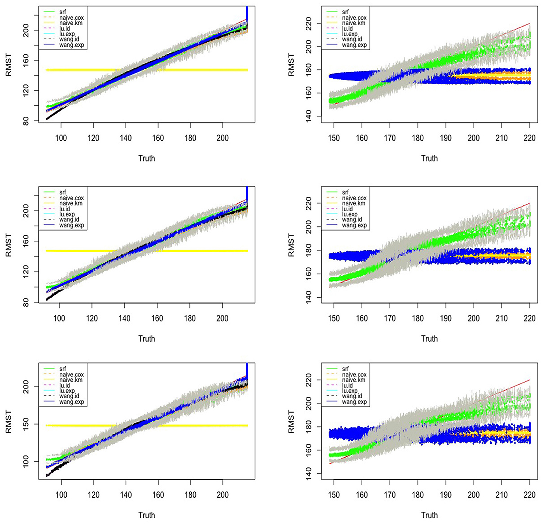
Figure 4. Estimated vs. the true RMST for Model 1 (left) and Model 2 (right) with exponential link function and the number of covariates p = 5, 10, 20 (top–bottom). SRF, proposed random forest-bases estimator, and upper and lower bounds of the point-wise confidence intervals of the proposed random forest estimator are connected in the gray lines; Naive.km, estimate based on Kaplan–Meier estimator without adjusting for the covariates; Naive.Cox, Cox regression based estimator; Lu.id, method of Tian et al. (2014) with identity link; Lu.exp, method of Tian et al. (2014) with exponential link; Wang.id, method of Wang and Schaubel (2018) with identity link; Wang:exp, method of Wang and Schaubel (2018) with exponential link.

Tables 1, 2 show the MAE and RMSE for Model 1 and Model 2, respectively. For Model 1, the parametric models are correctly specified using the methods of Tian et al. (2014); Wang and Schaubel (2018), we expect that both methods perform well, and our method can have a comparable performance. For Model 2, our proposed method dominates all other methods. Increasing the number of non-predictive covariates does not have a big impact on the performance of our method.

TABLE 1

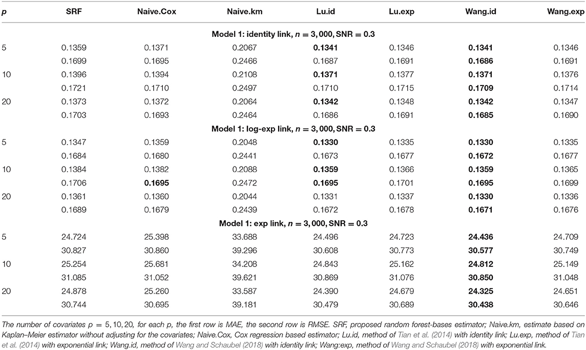
Table 1. Comparison of Mean-Absolute-Error (MAE) and Rooted-Mean-Squared-Error (RMSE) for Model 1 with different link functions.

TABLE 2

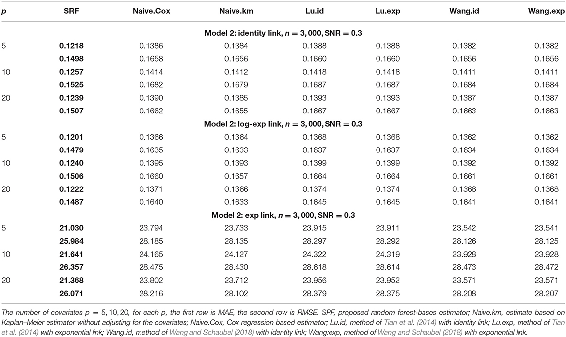
Table 2. Comparison of mean-absolute-error (MAE) and rooted-mean-squared-error (RMSE) for Model 2 with different link functions.

When the censoring distribution does not follow PH assumption, we may expect a difference in the prediction performance because of the bias of IPCW from mis-specification. To check whether our method can still outperform the existing methods, we conduct additional numerical studies. In particular, we simulate the censoring time from the following gamma distributions

$C~\Gamma (\alpha ,\beta ),\beta =\frac{1}{{\lambda }_{C}exp(X_{1}log2)},\text{ and }\alpha \in \left\{0.5,1.5\right\}$

When α = 1, the gamma distribution degenerates to the exponential distribution we used for Tables 1, 2. Tables 3, 4 show the MAE and RMSE for Model 1 and Model 2 when α = 0.5, and Tables 5, 6 show the MAE and RMSE for Model 1 and Model 2 when α = 1.5. Results of α ∈ {0.5, 1.5} are not very different from the results of α = 1. Under Model 1, our method performs comparably well as methods of Tian et al. (2014); Wang and Schaubel (2018), and it dominates the others under Model 2. When feature dimension is low(p = 5), the error metrics of our method when α = 1 are in general lower than the error metrics when α = 0.5, 1.5 for both Model 1 and Model 2. The additional errors can be regarded as the bias induced from the violation of PH assumption of the censoring distribution. When feature dimension is high(p = 10, 20), bias from large p may dominate the bias from the violation of PH assumption of the censoring distribution.

TABLE 3

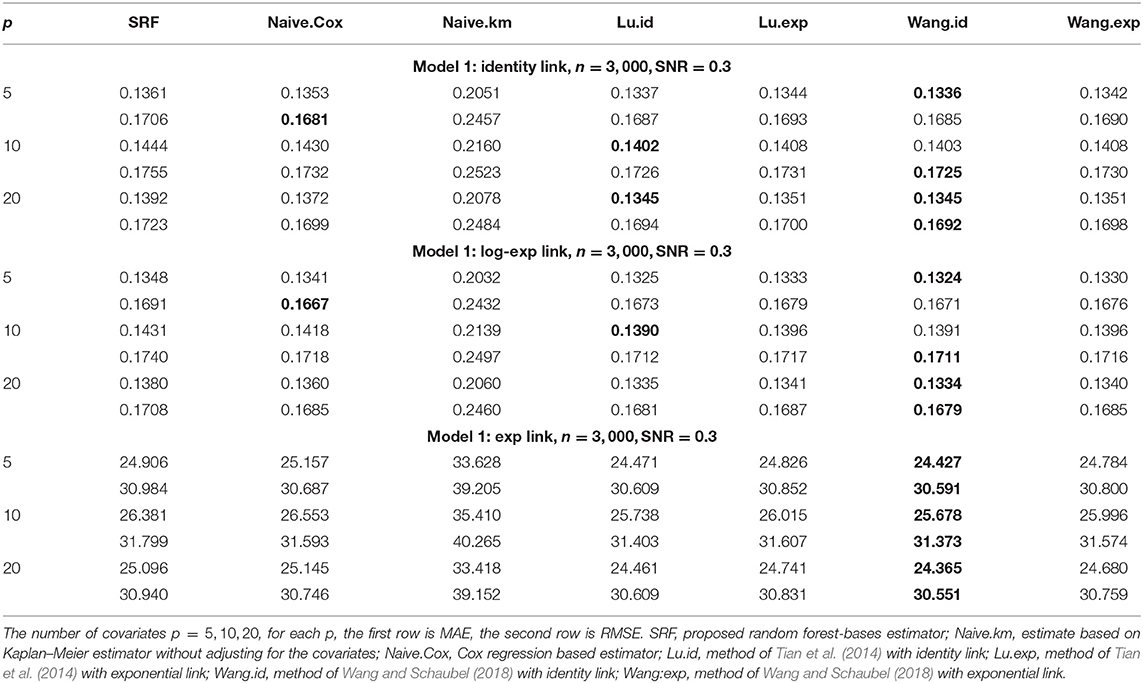
Table 3. Comparison of Mean-Absolute-Error (MAE) and Rooted-Mean-Squared-Error (RMSE) for Model 1 with different link functions and the censoring distribution is mis-specified with α = 0.5.

TABLE 4

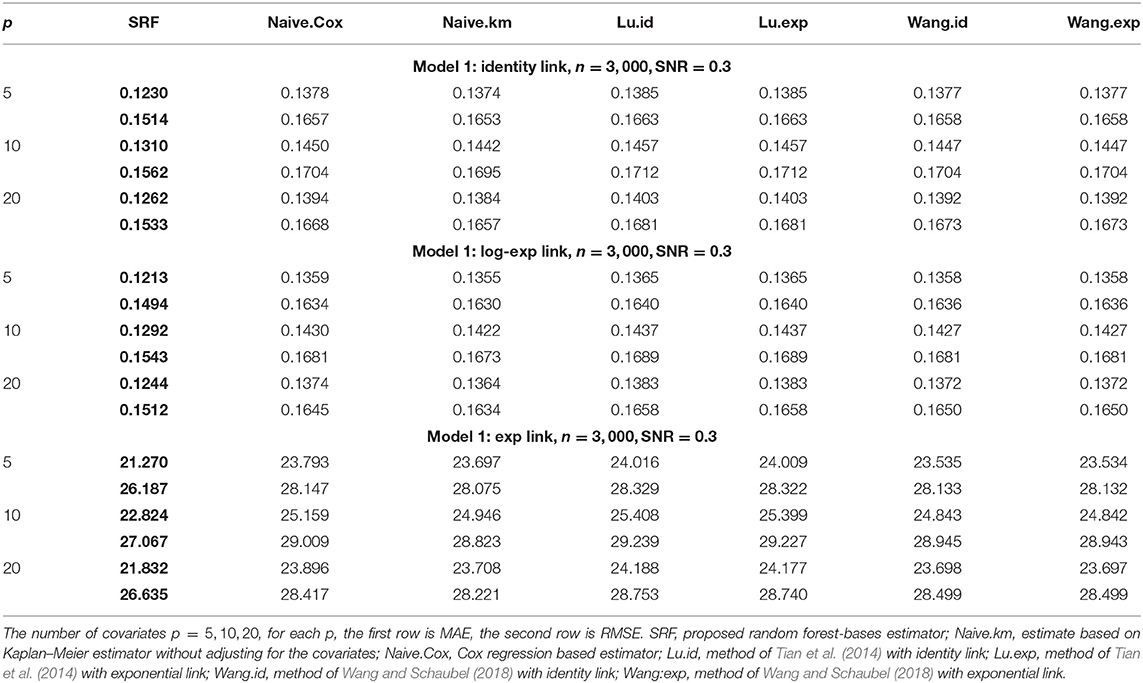
Table 4. Comparison of Mean-Absolute-Error (MAE) and Rooted-Mean-Squared-Error (RMSE) for Model 2 with different link functions and the censoring distribution is mis-specificed with α = 0.5.

TABLE 5

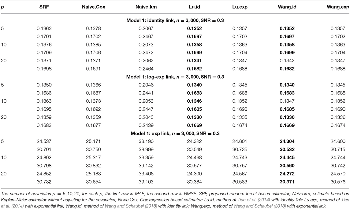
Table 5. Comparison of Mean-Absolute-Error (MAE) and Rooted-Mean-Squared-Error (RMSE) for Model 1 with different link functions and the censoring distribution is mis-specificed with α = 1.5.

TABLE 6

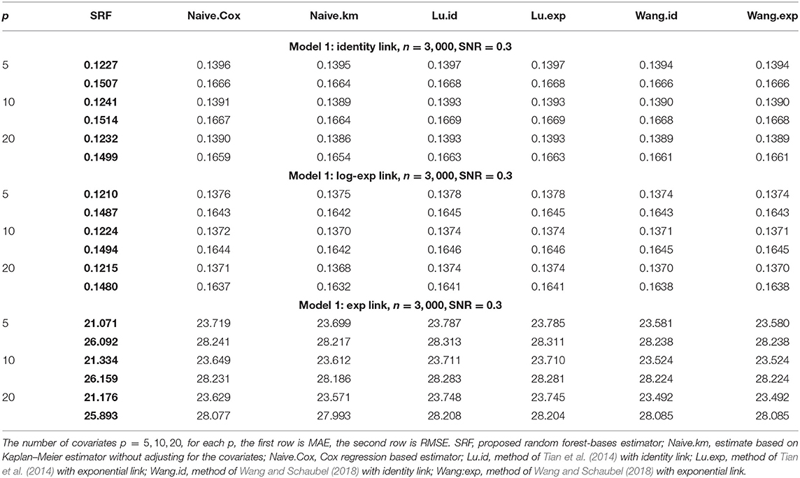
Table 6. Comparison of Mean-Absolute-Error (MAE) and Rooted-Mean-Squared-Error (RMSE) for Model 2 with different link functions and the censoring distribution is mis-specificed with α = 1.5.

5. Application to the TCGA Ovarian Cancer Data Set

We apply the proposed method to The Cancer Genome Atlas (TCGA) ovarian cancer functional proteomics data set (Akbani et al., 2015) that is publicly available (http://gdac.broadinstitute.org). The data sets include proteomic characterization of tumors using reverse-phase protein arrays (RPPA). Specifically, Akbani et al. (2015) reported an RPPA-based proteomic analysis using 195 high-quality antibodies that target total, cleaved, acetylated and phosphorylated forms of proteins in 412 high-grade serous ovarian cystadenocarcinoma (OVCA) samples. The function space covered by the antibodies used in the RPPA analysis emcompasses major functional and signaling pathways of relevance to human cancer, including proliferation, DNA damage, polarity, vesicle function, EMT, invasiveness, hormone signaling, apoptosis, metabolism, immunological, and stromal function as well as transmembrane receptors, integrin, TGFβ, LKB1/AMPK, TSC/mTOR, PI3K/Akt, Ras/MAPK, Hippo, Notch, and Wnt/beta-catenin signaling (Akbani et al., 2015).

After removing a few samples with missing data, the final data set includes 407 OVCA samples with a mean/median follow-up of 3.20/2.79 years and a total of 242 deaths and 40% censoring. To assess how different methods predict the hRMST, we performed the following cross-validation analysis. For a given L, we did 10-fold cross-validation on the data set. For each training data set in the cross-validation, we perform a univariate analysis to select top 5 most significant features based on univariate Cox regression analysis. We then estimate the hRMST on the test set using the training data sets with these 5 features as the predictors. We apply 7 different methods, including estimate based on the KM estimator, estimate based on the Cox model, the method of Tian et al. (2014) and the method of Wang and Schaubel (2018). We report the average of MAE and RMSE on the samples in the testing sets over the 10-fold cross-validation.

The results are shown in Table 7 and Figure 5 for L = 3, 4, 5 (see Supplementary Material for L = 6, 7, 8). There are 45.9, 31.2, 19.4, 11.8, 8.1, 4.4% of the observations larger than L for L = 3, 4, 5, 6, 7, 8 correspondingly. For different choices of L, our proposed random forest based method dominates the other methods in MAE and RMSE. The methods of Tian et al. (2014) and Wang and Schaubel (2018) are based on parametric form of hRMST. Cox model is heavily dependent on the proportional hazard assumption, and the Kaplan–Meier approach does not take the covariates into account. We also notice that the method of Wang and Schaubel (2018) always performs better than the method of Tian et al. (2014), possibly due to the fact that the censoring mechanism in the data depends on the covariates.

TABLE 7

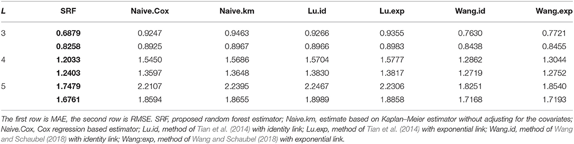
Table 7. Performance of the proposed random forest estimator compared with other methods for L = 3, 4, 5.

FIGURE 5

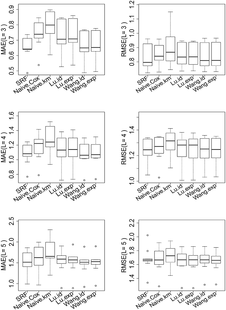
Figure 5. Performance of the proposed random forest estimator compared with other methods for L = 3, 4, 5. The left penal is the MAE across of 10-fold cross-validation. The right panel is the RMSE across of 10-fold cross-validation. SRF, proposed random forest estimator; Naive.km, estimate based on Kaplan–Meier estimator without adjusting for the covariates; Naive.Cox, Cox regression based estimator; Lu.id, method of Tian et al. (2014) with identity link; Lu.exp, method of Tian et al. (2014) with exponential link; Wang.id method of Wang and Schaubel (2018) with identity link; Wang:exp, method of Wang and Schaubel (2018) with exponential link.

6. Discussion

In this paper, we have developed a non-parametric random forest-based method for estimation of hRMST. Compared with traditional Cox model, which gets hRMST estimates by transforming the estimated hazard functions, directly modeling hRMST would be more preferable for computation and feature importance analysis. The proposed estimator can relax the parametric assumptions imposed on the survival time used in Tian et al. (2014) and Wang and Schaubel (2018), and can achieve better prediction performance. We have derived the asymptotic distribution of the random forest estimator using IPCW approach, and presented a procedure based on bags of little bootstraps to obtain the variance of the estimator. Our simulation results and analysis of TCGA data sets have shown promising performance in predicting hRMST as compared to the other available methods, even when the dimension is high and the covariates include irrelevant variables. The method is implemented by R and C++, and is available at https://github.com/lmy1019/SRF.

The proposed method can be used to estimate the heterogeneous treatment effects in randomized clinical trials when the outcome is censored. One can simply apply the method separately to the treated group and the placebo group and take the difference. However, for the observational studies, one needs to account for the fact that the treatment assignments might not be completely at random. Wager and Athey (2015) developed a non-parametric causal forest for estimating heterogeneous treatment effects that extends Breiman's random forest algorithm. In the potential outcomes framework with non-confounding, they showed that causal forest are pointwise consistent for the true treatment effect and have an asymptotically Gaussian and centered sampling distribution. For the observational studies with censored survival outcomes, it is also possible to combine the methods proposed here and the method of Wager and Athey (2015) in order to estimate the treatment effect on the restricted mean survival time.

The proposed methods can also be extended to take into account possible competing risk. This can be done by introducing an additional inverse probability weight (IPCW) to differentiate the non-informative censoring and competing risk censoring. In this case, the estimation equation ψ function with covariates history $\tilde{X}=\tilde{x}$ under true G_C and G_R becomes

$\begin{array}{l}{\tilde{\psi }}_{\mu }(\tilde{x},Z^L,{\delta }^L)=\frac{1}{1-G_C(Z^L|X=x)}\frac{1}{1-G_R(Z^L|\tilde{X}=\tilde{x})}\\ {\delta }^L(Z^L-\mu ),& (8)\end{array}$

where under competing risk scenario, ${\delta }^L=1_{\left\{T\wedge L\le C\wedge R\right\}}$. The method proposed in this paper can be automatically adapted to the competing risk case and the asymptotic normality result can be derived similarly.

Data Availability Statement

The original contributions presented in the study are included in the article/Supplementary Materials, further inquiries can be directed to the corresponding author/s.

Author Contributions

ML and HL developed the ideas and the methods together, analyzed the real data sets, and wrote the manuscript. ML implemented the methods and performed the numerical analysis. All authors contributed to the article and approved the submitted version.

Funding

This research was funded by NIH grants GM123056 and GM129781.

Conflict of Interest

The authors declare that the research was conducted in the absence of any commercial or financial relationships that could be construed as a potential conflict of interest.

Supplementary Material

The Supplementary Material for this article can be found online at: https://www.frontiersin.org/articles/10.3389/fgene.2020.587378/full#supplementary-material

References

Akbani, R., Ng, P. K. S., Werner, H. M., Shahmoradgoli, M., Zhang, F., Ju, Z., et al. (2015). Corrigendum: a pan-cancer proteomic perspective on the Cancer Genome Atlas. Nat. Commun. 6:5852. doi: 10.1038/ncomms5852

PubMed Abstract | CrossRef Full Text | Google Scholar

Andersen, P. K., and Gill, R. D. (1982). Cox's regression model for counting processes: a large sample study. Ann. Stat. 10, 1100–1120. doi: 10.1214/aos/1176345976

CrossRef Full Text | Google Scholar

Athey, S., Tibshirani, J., and Wager, S. (2018). Generalized Random Forests. Technical report. Stanford, CA: Stanford University.

Google Scholar

Biau, G. (2012). Analysis of a random forests model. J. Mach. Learn. Res. 13, 1063–1095.

Google Scholar

Biau, G., Devroye, L., and Lugosi, G. (2008). Consistency of random forests and other averaging classifiers. J. Mach. Learn. Res. 9, 2015–2033.

Google Scholar

Biau, G., and Scornet, E. (2016). A random forest guided tour. Test 25, 197–227. doi: 10.1007/s11749-016-0481-7

CrossRef Full Text | Google Scholar

Breiman, L. (2001). Random forests. Mach. Learn. 45, 5–32. doi: 10.1023/A:1010933404324

CrossRef Full Text | Google Scholar

Breiman, L. (2004). Consistency for a Simple Model of Random Forests. Technical report 670. Statistics Department, University of California at Berkeley.

Google Scholar

Chen, P. Y., and Tsiatis, A. A. (2001). Causal inference on the difference of the restricted mean lifetime between two groups. Biometrics 57, 1030–1038. doi: 10.1111/j.0006-341X.2001.01030.x

PubMed Abstract | CrossRef Full Text | Google Scholar

Cox, D. (1972). Regression models and life-tables. J. R. Stat. Soc. Ser, B 34, 187–220. doi: 10.1111/j.2517-6161.1972.tb00899.x

CrossRef Full Text | Google Scholar

Cox, D. (1975). Partial likelihood. Biometrika 62, 269–276. doi: 10.1093/biomet/62.2.269

CrossRef Full Text | Google Scholar

Cutler, D., Edwards, T. C., Beard, K., Cutler, A., Hess, K., Gibson, J., and Lawler, J. (2007). Random forests for classification in ecology. Ecology 8811, 2783–2792.

PubMed Abstract | Google Scholar

Davison, A., and Hinkley, D. V. (1997). Bootstrap Methods and Their Application. Cambridge University Press. Available online at: https://www.cambridge.org/core/books/bootstrap-methods-and-their-application/ED2FD043579F27952363566DC09CBD6A. doi: 10.1017/CBO9780511802843

CrossRef Full Text | Google Scholar

Denil, M., Matheson, D., and De Freitas, N. (2014). “Narrowing the gap: random forests in theory and in practice,” in Proceedings of The 31st International Conference on Machine Learning, 665–673. Available online at: http://proceedings.mlr.press/v32/denil14.html

Google Scholar

Díaz-Uriarte, R., and Alvarez de Andrés, S. (2006). Gene selection and classification of microarray data using random forest. BMC Bioinformatics 7:3. doi: 10.1186/1471-2105-7-3

PubMed Abstract | CrossRef Full Text | Google Scholar

Erfon, B. (1980). The Jackknife, the Bootstrap, and Other Resampling Plans. Available online at: https://statistics.stanford.edu/research/jackknife-bootstrap-and-other-resampling-plans

Google Scholar

Fang, E. X., Ning, Y., and Liu, H. (2017). Testing and confidence intervals for high dimensional proportional hazards model. J. R. Stat. Soc. Ser. B. 79, 1415–1437. doi: 10.1111/rssb.12224

CrossRef Full Text | Google Scholar

Friedberg, R., Tibshirani, J., Athey, S., and Wager, S. (2018). Local linear forests. J. Comput. Graph. Stat. 1–25. doi: 10.1080/10618600.2020.1831930

CrossRef Full Text | Google Scholar

Gill, R. D., and Gill, R. D. (1984). Understanding Cox's regression model: a martingale approach. J. Am. Stat. Assoc. 79, 441–447. doi: 10.1080/01621459.1984.10478069

CrossRef Full Text | Google Scholar

Hastie, T., Tibshirani, R., and Friedman, J. (2001). The Elements of Statistical Learning. New York, NY: Springer New York Inc. Available online at: https://www.bibsonomy.org/bibtex/2f58afc5c9793fcc8ad8389824e57984c/sb3000. doi: 10.1007/978-0-387-84858-7

CrossRef Full Text | Google Scholar

Huang, J., Sun, T., Ying, Z., Yu, Y., and Zhang, C. H. (2013). Oracle inequalities for the lasso in the cox model. Ann. Stat. 41, 1142–1165. doi: 10.1214/13-AOS1098

PubMed Abstract | CrossRef Full Text | Google Scholar

Ishwaran, H., and Kogalur, U. B. (2011). Consistency of random survival forests. Stat. Probab. Lett. 80, 1056–1064. doi: 10.1016/j.spl.2010.02.020

PubMed Abstract | CrossRef Full Text | Google Scholar

Ishwaran, H., Kogalur, U. B., Blackstone, E. H., and Lauer, M. S. (2008). Random survival forests. Ann. Appl. Stat. 2, 841–860. doi: 10.1214/08-AOAS169

CrossRef Full Text | Google Scholar

Meinshausen, N. (2006). Quantile regression forests. J. Mach. Learn. Res. 7, 983–999.

Google Scholar

Mentch, L., and Hooker, G. (2016). Quantifying uncertainty in random forests via confidence intervals and hypothesis tests. J. Mach. Learn. Res. 17, 26:1–26:41.

Google Scholar

Royston, P., and Parmar, M. K. B. (2013). Restricted mean survival time: an alternative to the hazard ratio for the design and analysis of randomized trials with a time-to-event outcome. BMC Med. Res. Methodol. 13:152. doi: 10.1186/1471-2288-13-152

PubMed Abstract | CrossRef Full Text | Google Scholar

Sexton, J., and Laake, P. (2009). Standard errors for bagged and random forest estimators. Comput. Stat. Data Anal. 53, 801–811. doi: 10.1016/j.csda.2008.08.007

CrossRef Full Text | Google Scholar

Steingrimsson, J. A., Diao, L., and Strawderman, R. L. (2019). Censoring unbiased regression trees and ensembles. J. Am. Stat. Assoc. 114, 370–383. doi: 10.1080/01621459.2017.1407775

PubMed Abstract | CrossRef Full Text | Google Scholar

Svetnik, V., Culberson, J. C., Tong, C., Cullberson, J. C., Sheridan, R. P., and Feuston, B. P. (2003). Random forest: a classification and regression tool for compound classification and QSAR modeling. J. Chem. Inform. Comput. Sci. 43, 1947–1958. doi: 10.1021/ci034160g

PubMed Abstract | CrossRef Full Text | Google Scholar

Tian, L., Tianxi, C., Goetghebeur, E., and Wei, L. J. (2007). Model evaluation based on the sampling distribution of estimated absolute prediction error. Biometrika 2, 297–311. doi: 10.1093/biomet/asm036

CrossRef Full Text | Google Scholar

Tian, L., Zhao, L., and Wei, L. J. (2014). Predicting the restricted mean event time with the subject's baseline covariates in survival analysis. Biostatistics 15, 222–233. doi: 10.1093/biostatistics/kxt050

PubMed Abstract | CrossRef Full Text | Google Scholar

Wager, S., and Athey, S. (2015). Estimation and inference of heterogeneous treatment effects using random forests. J. Am. Stat. Assoc. 113, 1228–1242. doi: 10.1080/01621459.2017.1319839

CrossRef Full Text | Google Scholar

Wang, X., and Schaubel, D. E. (2018). Modeling restricted mean survival time under general censoring mechanisms. Lifetime Data Anal. 24, 176–199. doi: 10.1007/s10985-017-9391-6

PubMed Abstract | CrossRef Full Text | Google Scholar

Zhang, M., and Schaubel, D. E. (2011). Estimating differences in restricted mean lifetime using observational data subject to dependent censoring. Biometrics 67, 740–749. doi: 10.1111/j.1541-0420.2010.01503.x

PubMed Abstract | CrossRef Full Text | Google Scholar

Zucker, D. M. (1998). Restricted mean life with covariates: modification and extension of a useful survival analysis method. J. Am. Stat. Assoc. 93, 702–709. doi: 10.1080/01621459.1998.10473722

CrossRef Full Text | Google Scholar