Predominant Atmospheric and Oceanic Patterns during Coastal Marine Heatwaves

1. Introduction

Extreme thermal events that occur in the ocean are classified here as “marine heatwaves” (MHWs) after Hobday et al. (2016). These events may occur suddenly, anywhere in the world, and at any time of the year. Several large MHWs, and their ecological impacts, have already been well documented. One of the first MHWs characterized occurred in 2003, and it negatively impacted as much as 80% of the Gorgonian fan colonies in the Mediterranean (Garrabou et al., 2009). A 2011 MHW is now known to have caused a permanent range contraction by roughly 100 km of the ecosystem forming-kelp species Ecklonia radiata in favor of the tropicalisation of reef fishes and seaweed turfs along the southern coast of Western Australia (Wernberg et al., 2016). The damage caused by MHWs is not only confined to demersal organisms or coastal ecosystems, e.g., a MHW in the North West Atlantic Ocean in 2012 indicated that these kinds of extreme events are also able to impact multiple commercial fisheries (Mills et al., 2013). When extreme enough, such as “The Blob” that persisted in the North West Pacific Ocean from 2014 to 2016, a MHW may negatively impact even marine mammals and seabirds (Cavole et al., 2016). Besides increases in mortality due to thermal stress, MHWs may also lead to outbreaks of disease in commercially viable species, such as that which occurred during the 2015/16 Tasman Sea event (Oliver et al., 2017a).

It is now possible to directly compare MHWs occurring anywhere on the globe during any time of year using a statistical methodology developed by Hobday et al. (2016) that defined these events as “a prolonged discrete anomalously warm water event that can be described by its duration, intensity, rate of evolution, and spatial extent.” Whereas the metrics created for the measurement of MHWs allowed for the comparison of events, they did not directly reveal what may be causing them. Beyond common measurements, it is necessary to determine the predominant patterns that occur during MHWs in order to identify their physical drivers.

It has been assumed that coastal MHWs should either be caused by oceanic forcing, atmospheric forcing, or a combination of the two; however, the scale at which this forcing must occur in order to drive MHWs at the coast has yet to be determined. Recent research into the rates of co-occurrence between nearshore and offshore MHWs revealed that oceanic forcing from offshore (broad-scale) onto the nearshore (<400 m from the coast, i.e., also referred to as local-scale) was far less responsible for the formation of coastal MHWs than hypothesized (Schlegel et al., 2017). It is therefore necessary to consider broader meso-scale mechanisms that may be responsible for such events occurring at the local-scale. For example, the 2011 Western Australia MHW (Pearce and Feng, 2013) was caused by the aseasonal transport of warm water onto the coast due to a surge of the Leeuwin Current (Feng et al., 2013; Benthuysen et al., 2014). Oceanic forcing was also the main contributor of the anomalously warm water during the 2015/16 Tasman MHW when the southward flowing East Australian Current caused a convergence of heat there (Oliver et al., 2017a). Conversely, Garrabou et al. (2009) were able to show that atmospheric forcing played a clear role in formation of the 2003 Mediterranean MHW. While more complex, Chen et al. (2015) also showed that atmosphere-ocean heat flux could be attributed as the main forcing variable in the 2012 Atlantic MHW. The Blob, however, appears to have occurred due to the lack of advection of heat from surface waters into the atmosphere due to anomalously high sea level pressure (Bond et al., 2015). Outside of these few examples for these well documented events there has been little progress in developing a global understanding of the forcing of MHWs, nor has a methodology been developed with the capacity to determine the probable drivers of multiple MHWs simultaneously.

In order to develop a methodology that could be used to investigate the potential atmospheric and/or oceanic forcing of multiple coastal MHWs within a single framework, an index of the mean synoptic atmospheric and oceanic states around southern Africa during the occurrence of these events was created, similar to Oliver et al. (2017b) for Eastern Tasmania. The daily climatology for the atmosphere and ocean around southern Africa were also calculated to determine if the MHW states differed from the expected daily values. After determining this distinction, the MHW states were clustered with the use of a self-organizing map (SOM). The aim of the distinction and the clustering was to visualize meso-scale patterns in the atmosphere and/or ocean that occur during MHWs at coastal sites, and to be certain that these patterns were different from daily climatologies. We predicted that (i) atmospheric and oceanic states during MHWs would differ from daily climatology states; (ii) recurrent atmospheric and oceanic patterns would be revealed through clustering; and (iii) the clustered patterns would aid in the development of a broader mechanistic understanding of the physical drivers of coastal MHWs.

2. Materials and Methods

2.1. Study Region

The ca. 3,100 km long South African coastline provides a natural laboratory for investigations into the forcing of nearshore phenomena as it may be divided into three distinct sections, allowing for a range of meso-scale oceanic influences to be considered within the same research framework (Figure 1); therefore, the extent of the study area was set at 10 to 40°E and 25 to 40°S. The range of sea surface temperatures experienced along all three coasts is large, and the gradient of increasing temperature from the border of Namibia (Site 1) to the border of Mozambique (Site 26) is nearly linear. The west coast of the country is distinct from the other two coasts as it is bordered by the Benguela Current, which forms an Eastern Boundary Upwelling System (EBUS) (Hutchings et al., 2009) against the coast. Conversely, the east coast is dominated by a western boundary current, the Agulhas Current (Lünning, 1990), a poleward flowing body of warm water. The south coast is also bordered by the Agulhas Current, but differs from the east coast in that it experiences both shear-forced and wind-driven upwelling (Lutjeharms et al., 2000) in addition to having significantly more thermal variability than the other two coasts (Schlegel et al., 2017). The Agulhas and Benguela currents meet along the south coast of the subcontinent, and rather than having a fixed border, the two range from the Cape Peninsula in the west, to the western portion of the Agulhas Bank in the east. The Agulhas Current retroflects upon coming into contact with the Benguela (Hutchings et al., 2009); however, it will occasionally punch through into the South Atlantic. This event, known as Agulhas leakage, allows warm, saline eddies of Indian Ocean water to propagate into the Atlantic Ocean (Beal et al., 2011).

FIGURE 1

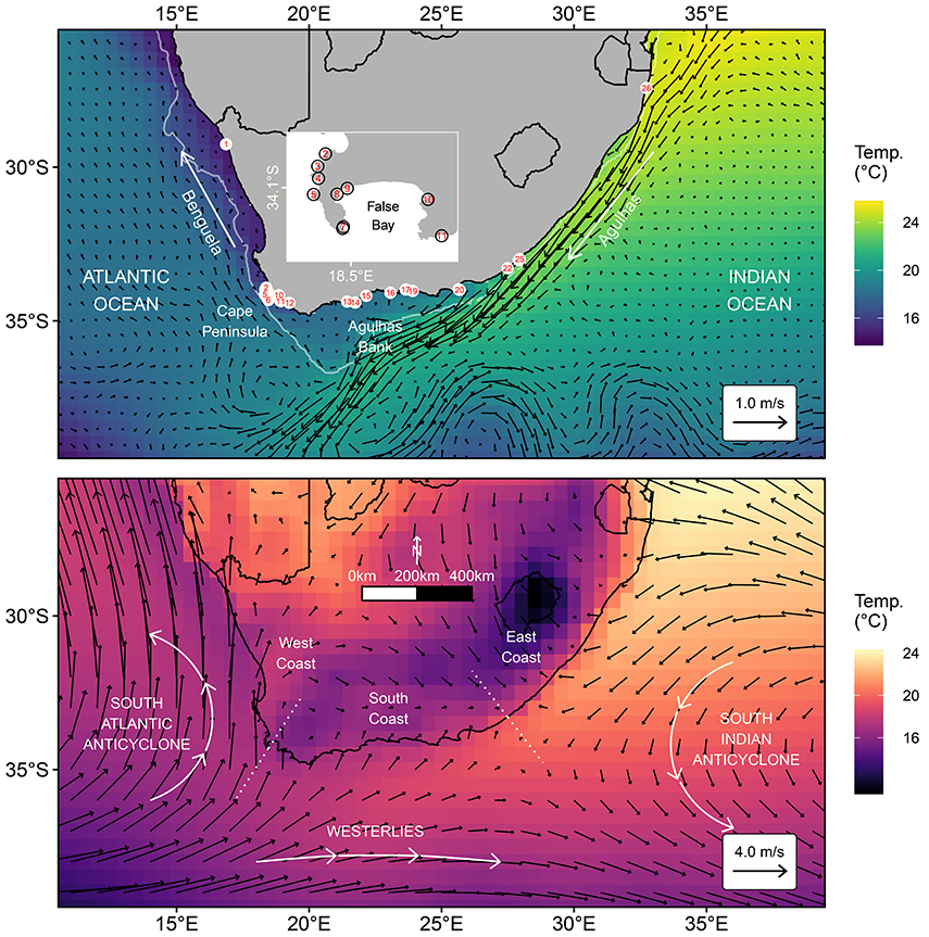
Figure 1. Map of the study area where the top panel shows the mean annual sea surface temperature (SST) and surface currents from 1993 to 2016, as well as the locations referred to in the text. The sites of in situ collection are shown with red numerals over white circles. An inset map of the Cape Peninsula/False Bay area is shown where site labels are obscured due to overplotting. The bottom panel shows the mean surface atmospheric temperature and winds, and highlights the three coastal sections found within the study area as well as the three predominant wind patterns. Note that the temperature and vector scales differ between the two panels. The white vector arrows showing the predominant ocean and atmosphere circulation patterns are approximations and not exact values.

Atmospheric circulation over the study area is dominated by two quasi-stationary anticyclonic high pressure cells. The South Indian Ocean High (hereafter Indian high) is situated approximately on the eastern border of the study area and draws warm moist air toward the east coast, whereas the South Atlantic Ocean High (hereafter Atlantic high) is found to the west of the subcontinent and draws cool dry air onto the west coast (Van Heerden and Hurry, 1998). To the south of the subcontinent, prevailing westerly winds blow south of these two high pressure cells (Van Heerden and Hurry, 1998). From their annual mean mean wind patterns, these three atmospheric features can be discerned from Figure 1. Summer heating may lead to the development of heat lows within the subcontinent, which tend to be absent during winter (Tyson and Preston-Whyte, 2000), allowing for the Indian and Atlantic highs to link over land (Van Heerden and Hurry, 1998). Additionally, the Indian and Atlantic highs, as well as the westerlies, move northwards during winter months, with the effect that the colder westerly winds influence the weather mostly along the southern parts of the sub-continent (Van Heerden and Hurry, 1998). Atmospheric temperatures along the coasts are largely influenced by the cold Benguela on the west coast and warm Agulhas Current along the east and south coasts (Van Heerden and Hurry, 1998).

2.2. Data

2.2.1. Atmospheric Data

To visualize a synoptic view of the atmospheric state around southern Africa during coastal MHWs (see sections “Marine heatwaves” and “Atmosphere-ocean state” below), we chose to use ERA-Interim to provide atmospheric temperatures (2 m above surface) and wind vectors (10 m above surface). ERA-Interim is a comprehensive global atmospheric model that assimilates a wide range of data to create short term forecasts for 60 vertical layers (Dee et al., 2011). These forecasts are then combined with the assimilated data again during each 12-hourly cycle (Dee et al., 2011). ERA-Interim is produced by the European Center for Medium-Range Weather Forecasts (ECMWF, http://www.ecmwf.int/), and at the time of this writing the chosen variables were available for download from January 1st, 1979 to December 31st, 2016. The data used in this study were downloaded at a daily resolution on a 1/2°  grid and within the latitude/longitude of the study region (Figure 1).

2.2.2. Oceanic Data

The in situ coastal seawater temperature data used in this study were acquired from the South African Coastal Temperature Network (SACTN)¹. These data are contributed by seven different organizations and are collected in situ with a mixture of hand-held alcohol or mercury thermometers as well as digital underwater temperature recorders (UTRs). This data set currently consists of 135 daily time series, with a mean duration of 19.7 years, meaning that many the time series in this dataset are shorter than the 30 year minimum proscribed for the characterisation of MHWs (see “Marine heatwaves” section below) (Hobday et al., 2016). It is however deemed necessary to use these data when investigating extreme events in the nearshore (<400 m from the low tide mark) as satellite derived sea surface temperature (SST) values along the coast have been shown to display large biases (Smit et al., 2013) or capture minimum and maximum temperatures poorly (Smale and Wernberg, 2009; Castillo and Lima, 2010). Whereas a 30+ year period is ideal for determining a climatology, 10 years may serve as an acceptable bottom limit (Schlegel et al., 2017). Following on from the methodology laid out in Schlegel et al. (2017), time series with more than 10% missing data or shorter than 10 years in length were excluded from this research. Accounting for these 10 year length and 10% missing data constraints, the total number of in situ time series used in this study was reduced to 26, with a mean length of 22.3 years.

Research on oceanic reanalysis data around southern Africa have shown that none of the products currently available model the complex Agulhas Current well (Cooper, 2014). It was therefore decided to use remotely sensed data to determine the SST and surface currents in the study area.

SST within the study region was determined with the AVHRR-Only Optimum Interpolated Sea Surface Temperature (OISST) dataset produced by NOAA. NOAA OISST is a global 1/4°  gridded daily SST product that assimilates both remotely sensed and in situ sources of data to create a level-4 gap free product (Banzon et al., 2016). These data were averaged to a 1/2°  grid to match the courser resolution of the ERA-Interim data. At the time of this writing these data were available for download from September 1st, 1981 to June 5th, 2017.

To determine ocean surface currents remotely on a daily global 1/4°  grid, sea level anomaly (SLA) values are used to determine absolute geostrophic flows. The directional values of these flow vectors (U and V) were the values used in this study. These values were averaged to a 1/2°  grid to maintain consistent spatial representation between the datasets. At the time of this writing these data were available from January 1st, 1993 to January 6th, 2017. These altimeter products were produced by Ssalto/Duacs and distributed by Aviso, with support from Cnes (http://www.aviso.altimetry.fr/duacs/).

2.3. Marine Heatwaves (MHWs)

We use here the definition as well as the methodology laid out in Hobday et al. (2016) for the analysis of MHWs in this research. The algorithm developed by Hobday et al. (2016) requires daily time series data and isolates MHWs by first establishing the daily climatologies for the given time series. This is accomplished by finding the range of temperatures for any given day of the year, and then pooling these daily values further with the use of an 11-day moving window, across all years. From this pool are calculated two statistics of interest: the first is the average climatology for each day, and the second the 90th percentile threshold for each day. When the observed temperatures within a time series exceed this threshold for a number of days it may be classified as a discrete event. Perkins and Alexander (2013) concluded that the minimum duration for the analysis of atmospheric heatwaves was 3 days whereas Hobday et al. (2016) found that a minimum length of 5 days allowed for more uniform global results. It was also determined that any MHW that had “breaks' below the 90th percentile threshold lasting ≤2 days followed by subsequent days above the threshold were considered as one continuous event (Hobday et al., 2016). Previous work by Schlegel et al. (2017) showed that the inclusion of these short five day MHWs may lead to spurious connections between events found across different datasets. Therefore we have limited the inclusion of MHWs within this study to those with a duration in the top 10th percentile of all events that occurred within the range of complete years of data available for all of the datasets used in this study (1994–2016). Thus, from the 976 total MHWs detected in the in situ dataset, only 86 were used here.

In order to calculate a MHW it is necessary to supply a climatology against which daily values may be compared. It is proscribed in Hobday et al. (2016) that this period be at least 30 years. Because 20 of the 26 time series used here are below this threshold, we have opted to use the complete data period for each station as the climatological period. Using fewer than 30 years of data to determine a climatology prevents the accurate inclusion of any decadal scale variability (Schlegel and Smit, 2016); however, by using at least 10 years of data we are able to establish a baseline climatology to calculate MHWs (Schlegel et al., 2017). By calculating MHWs against the daily climatologies in this way, the amount they differ from their localities may be quantified and compared across time and space — the implication is that this allows researchers to examine events from different variability regimes (i.e., regions of the world, seasons) and compare them with a consistent set of MHW metrics. The definitions for the metrics that will be focused on in this paper may be found in Table 1.

TABLE 1

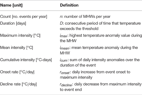
Table 1. The descriptions for the metrics of MHWs as proposed by Hobday et al. (2016) and adapted from Schlegel et al. (2017).

The MHWs in the SACTN dataset were calculated via the R package “RmarineHeatWaves” (Smit et al., 2017). This package implements the methodology detailed above, as first proposed by Hobday et al. (2016). The original algorithm used in Hobday et al. (2016) is available for use via python².

It is worth emphasizing that MHWs as defined here exist against the daily climatologies of the time series in which they are found and not by exceeding an absolute threshold. Therefore, one may just as likely find a MHW during winter months as summer months. This is a valuable characteristic of this method of investigation because aseasonal warm winter waters may, for example, have deleterious effects on relatively thermophobic species (Wernberg et al., 2011), or aid the recruitment of invasive species (Stachowicz et al., 2002).

It must also be clarified that due to the irregular sampling effort in the SACTN dataset along the coastline of southern Africa, the spatial and temporal distributions of the 86 MHWs are not necessarily even, with some areas, specifically the south coast, having a much greater likelihood of MHWs that meet the selection criteria. Addressing this imbalance would require that the use of data from the south coast (seventeen time series) be constrained to resemble that of the east coast (four time series) and west coast (five time series). This would reduce the number of time series used here roughly in half. Because the aim of this research was to determine the predominant atmospheric or oceanic states (see section “Atmosphere-Ocean States” below) during the longest events in the dataset, regardless of where or when they occurred, it was decided not to correct for this inequality in the data.

2.4. Atmosphere-Ocean States

In order to visualize meso-scale patterns in the atmosphere and ocean around southern Africa during a coastal MHW, it was necessary to first combine all of the daily values of these physical states for all days available across all of the datasets downloaded for this research (1994–2016). The oceanic states consisted of SST and surface currents while the atmospheric states were surface temperatures and surface winds. One mean atmosphere-ocean state was then created for each of the 86 MHWs in this study by taking the daily atmosphere-ocean states during each day during which the event occurred and averaging them together. For example, for a MHW that started on December 1st, 1999, and ended on March 7th, 2000, the 98 daily atmosphere-ocean states during that event were averaged to create a single atmosphere-ocean state that represented the overall pattern that was occurring during that one event. This example may be seen in the top row of panels in Figure 2.

FIGURE 2

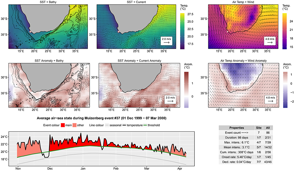
Figure 2. An atlas figure for a single coastal marine heatwave (MHW). The location of collection for the in situ coastal seawater temperature time series is shown in each of the top six panels as a white dot with a red border. The top row of panels shows the mean synoptic atmospheric and oceanic states during the MHW, created by averaging all daily synoptic atmosphere-ocean states during the event. The middle row shows anomalies for the mean atmospheric and oceanic states during the event. The left hand panel in the bottom row shows the period of the time series in which the MHW occurred. The table in the bottom right corner shows the values for the relevant metrics of the event as explained in Table 1 as well as its ranking against other events at the same site and the entire study area. Similar figures for each of the 86 MHWs used in this study are available here.

The calculation of the anomalies that would be used for all subsequent stages of this research required that a daily climatology be created for the atmospheric and oceanic states. These 366 daily atmosphere-ocean climatologies were calculated using the same algorithm used to determine the average daily climatologies for the in situ time series, with the climatological period set from 1994 to 2016 as this was the widest period available across all of the gridded datasets. With the atmosphere-ocean climatology known for each calendar day of the year, it was then possible to subtract these daily climatologies from the daily atmosphere-ocean states during which a MHW was occurring before averaging each individual daily anomaly together to create one mean atmosphere-ocean anomaly state for each event. An example of the atmosphere-ocean anomaly states created in this way may be seen in the middle row of Figure 2. The daily climatology anomaly states to be used for comparison against the MHW anomaly states (see section “Nonmetric multidimensional scaling (NMDS)” below) were created by subtracting the annual mean climatology state from all of the daily climatology states.

2.5. Nonmetric Multidimensional Scaling (NMDS)

The goal of using Nonmetric multidimensional scaling (NMDS) to ordinate the MHW anomaly states (hereafter MHW states) and climatology anomaly states (hereafter climatology states) was not to perform a statistical analysis on the data; indeed no significance is tested, but rather to visualize how each state relates to every other state while simultaneously visualizing the effects of the categorical variables on the data. The resultant biplot generated by NMDS allows one to visually inspect the relationship between MHW and climatology states, in order to determine if they share a common pattern, or are indeed dissimilar from one another. This is done by reducing the dimensionality of the atmosphere-ocean states down to a two-dimensional field that may be understood by mere humans. NMDS was chosen for this task over other ordination techniques, such as principal component analysis (PCA), as it may visualize all of the variance between the different states along only two axes, whereas PCA would only display part of that variance (Paliy and Shankar, 2016). NMDS is also one of the most robust unconstrained ordination methods available (Minchin, 1987). The use of this technique may not be wide-spread in climate science, but we found that it was effective for reducing the dimensionality of the atmosphere-ocean states used here. The temperature, U and V variables were first scaled to a mean of zero across the common variables within the same pixels for all MHW and climatology states. These scaled values were then converted into a Euclidean distance matrix before being fed into the NMDS algorithm. An additional benefit of NMDS is that it allows for the strength of the influence of the categorical variables within the data to be displayed on the resultant biplot as vectors, where the length of each vector represents the amount of influence that categorical variable has, and the direction of the vector shows where on the two-dimensional plain the ordinated data points are being influenced toward. The categorical variables considered when ordinating the MHW and climatology states together were the season during which the day or event occurred/started, as well as if the value represented a MHW or a climatology. The steps outlined here were conducted with algorithms from the R package “vegan”; (Oksanen et al., 2017).

It is important to note with NMDS that the two dimensions (i.e., x and y axes) along which all data points are ordinated do not represent any specific variables or quantities within the dataset. Instead these axes represent the algorithm's best attempt at reducing the stress in the model when constraining a multi-dimensional dataset into a two-dimensional visualization (Kruskal, 1964). It therefore requires knowledge of the data being ordinated in order for the user to determine a best approximation for the variables most closely represented in the axes of ordination.

2.6. Self-organizing Maps (SOMs)

Several methods of clustering synoptic data have been employed in climate science. Of these K-means clustering is perhaps most often employed (e.g., Corte-Real et al., 1998; Burrough et al., 2001; Kumar et al., 2011), with hierarchical cluster analysis (HCA) less so (e.g., Unal et al., 2003). A newer technique, self-organizing maps (SOMs), has been gaining in popularity in climate studies (e.g., Cavazos, 2000; Hewitson and Crane, 2002; Morioka et al., 2010). Here we have used a SOM to cluster the 86 MHW state anomalies.

The initialisation of a SOM is similar to more traditional clustering techniques (e.g., Jain, 2010) in that a given number of clusters (hereafter referred to as nodes) are declared by the user in order to instruct the SOM algorithm into how many nodes it should first randomly assign all of the data point (Hewitson and Crane, 2002). Each data point in this instance represents an atmosphere-ocean anomaly state during a MHW and consists of temperature, U and V anomalies, which reach a total 9774 variables each. Therefore, each SOM node is represented not by a single value, but by a 9774 value long reference vector. After all of the data points have been clustered into a node, the SOM then determines the most suitable reference vector for each node to represent the data therein (Hewitson and Crane, 2002). The data points are then reintroduced to the SOM and, based on Euclidean distance, each data point is then matched to the node of ‘best fit’ (Hewitson and Crane, 2002). During this process the reference vectors for each node are modified as the SOM algorithm “learns” how best to refine them to fit the data points, while also learning how best to fit the nodes in relation to one another (Hewitson and Crane, 2002). This means that not only does the SOM algorithm update the goodness of fit for each node during each run of the data, it also better orientates the nodes against one another and allows better clustering of higher densities of similar data points (MHW state anomalies) (Hewitson and Crane, 2002). This allows the user to see not only into which node a given data point (MHW state anomaly) best belongs in, but also what the relationship between the nodes may be and how prevalent certain MHW state anomalies are over others. Here we initially allowed the SOM algorithm to iterate this process 100 times. Analysis of the resultant SOM showed that little progress was made in the fitting of the data after 40 iterations, and so 100 iterations was deemed appropriate.

Because the SOM algorithm was not able to provide consistent results each time the analysis was run on these data, we opted out of using the default random initialisation (RI) method for the SOM in favor of principal component initialisation (PCI). PCI differs from RI in that it uses the two principal components of the dataset, as determined from a PCA to initialise the choice of node centers for the SOM (Akinduko et al., 2016). This allows the SOM model to recreate the same results when it is run on the same data. The SOM algorithm used in this study was taken from the R package ‘yasomi’ (Rossi, 2012).

The appropriate number of nodes to use in a cluster analysis is an important decision (Gibson et al., 2016). This is because it is necessary to include enough nodes to view a broad range of synoptic states, but not so many that the differences between the nodes become meaningless. Calculating the within group sum of squares (WGSS) as more nodes were included showed that four could be satisfactory, but that at least six would be better. Ultimately we settled on nine nodes as this allowed for a wider variety of different synoptic atmosphere-ocean states to be separated out from one another, allowing for a better understanding of the dominant patterns that exist during coastal MHWs. As proposed in Johnson (2013), the nodes that are output by a SOM should be significantly different from one another to ensure that an excess of nodes has not been used. Running an analysis of similarity we found this to be true for the choice of nine nodes (p = 0.001).

Once each MHW state anomaly was clustered into a node a further mean atmosphere-ocean state anomaly for each node was calculated by taking the average of all of the MHW state anomalies clustered within each node. It was these final mean atmosphere-ocean state anomalies that were taken as the nine predominant atmosphere-ocean patterns during coastal MHWs.

3. Results

3.1. Ordination of States

In order to determine any patterns in the differences between the MHW and climatology states, they were ordinated together using NMDS (stress = 0.14) and plotted on a biplot. Figure 3 shows that the climatology states were clustered together in a central position while the MHW states were scattered along the top and bottom. Furthermore, the climatology states have been ordinated by season in a very contiguous manner with little seasonal pattern existing for the MHW states. The vectors in Figure 3 showing the influence of the categorical variable “Season” very clearly relate to the occurrence of the climatology states, and not to the season of occurrence for the MHW states. The vectors indicating the direction of influence for the categorical variable “State” (i.e., MHW state or climatology state) show that the climatology states tend to center in the middle of the biplot, as we may see, but that the MHW states tend to be ordinated similarly toward states that occur during autumn months. It is important to remember that these results are in reality multi-dimensional, not two-dimensional as shown here. This is why Figure 3 shows MHW states both above and below the climatology states even though the vector for MHW states appears similar to the autumn vector. That the climatology states vary along the x axis in order of their occurrence throughout the year indicates that the variance this represents is the change in mean atmospheric and oceanic temperature throughout the seasonal cycle. The variance along the y axis is less clear, though it most likely represents differences in currents and winds. This inference is supported by the positioning of the spring and autumn climatology states, which are more variable than winter and summer, further up and down the y axis. There is also a significant (p = 0.002) relationship between the duration (days) of the MHW and its position along the y axis, with the shorter MHWs further from the center of the biplot. The MHW states are distributed either above the summer/spring climatology states or below the autumn climatology states. Furthermore, very few MHW states were near climatology states of the same season (e.g., winter MHW states may generally be found above the summer climatologies or below the autumn climatologies).

FIGURE 3

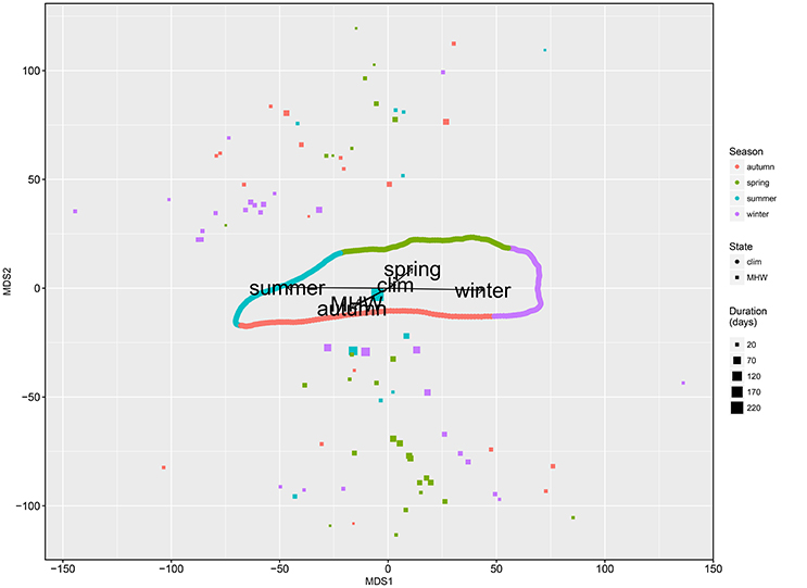
Figure 3. Biplot (stress = 0.14) showing the ordination of climatology (clim) states (circles) and marine heatwave (MHW) states (squares). The x and y axes are not representative of any specific values of the states, rather the distance between each point shows the best fitting relationship of all states with one another based on the output of a nonmetric multidimensional scaling (NMDS) model. The season of the year during which the state occurred/started is shown in color. The influence of the two categorical variables, type of atmosphere-ocean state and season of occurrence, on the placement of each state in the two-dimensional space are shown as black labeled vectors. Note that the clim states (circles) are plotted so tightly together that they do not appear as individual points. The duration of the MHW states (not the clim states) are indicated by the size of the square points.

3.2. SOM Nodes

The nine predominant atmospheric and oceanic patterns around southern Africa during coastal MHWs may be seen in Figure 4. Note that while the oceanic and atmospheric patterns for each node are shown in separate panels, all atmosphere and ocean variables were fed through the SOM together, meaning that the SOM had to consider both states when clustering them into nodes. The oceanic states appear to have been the most relevant criteria for clustering into the nodes in the top left corner, centered on Node 1, with nodes further away having less pronounced oceanic patterns. The nodes along the right edge, centered on Node 6, show that the primary influence for the clustering of MHW states there was the atmosphere. The further from Node 6 a node is placed, the less pronounced the atmospheric pattern becomes. The further from these two dominant points a node is, the less pronounced the patterns therein will become, as Node 7 shows.

FIGURE 4

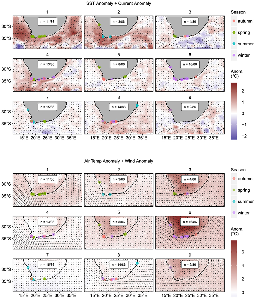
Figure 4. Predominant anomalous atmospheric and oceanic patterns during coastal marine heatwaves (MHWs) as determined by a SOM. The top nine panels show the oceanic patterns while the bottom nine panels show the atmospheric patterns. The current and wind vectors are the same scale as those found in the respective atmospheric and oceanic panels of Figure 1. The number of events clustered into each node is shown within the white label in the middle of each panel. The location of each coastal MHW within each node is shown with a dot whose color denotes the season during which that event occurred/started. Note that the temperature anomaly scales differ for the top and bottom nine panels.

MHWs that occurred during summer were the least common, only present in three nodes (Figure 5), with winter and spring events occurring more than twice as frequently (Table 2). Every node contained at least one spring event, and all but two nodes contained winter events. Three nodes lacked autumn events, but these were otherwise the most evenly distributed. Clustering of autumn, winter, and spring events that occurred over a range of years may be found in six of the nine nodes; however, the clustering of events that occurred within the same year is also consistent throughout the nodes. All but one of the nodes contained MHWs that were separated over large distances and by oceanographically dissimilar features. Additionally, only three of the 86 MHWs in this study occurred on the east coast and were clustered into nodes that had events from all three coasts.

FIGURE 5

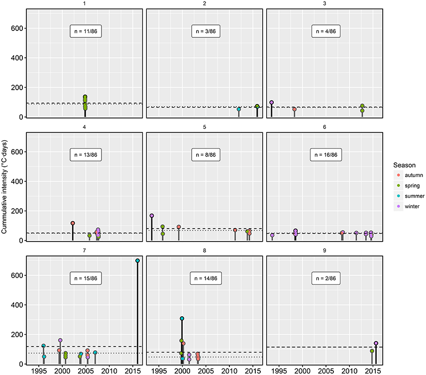
Figure 5. Lolliplot showing the start date for each marine heatwave (MHW) within each node as seen in Figure 4, with the portion of total events per node shown within the white label in the middle of each panel. The height of each lolli shows the cumulative intensity of the event, as outlined in Table 1, while the lolli color denotes the season during which the event occurred/started.

TABLE 2

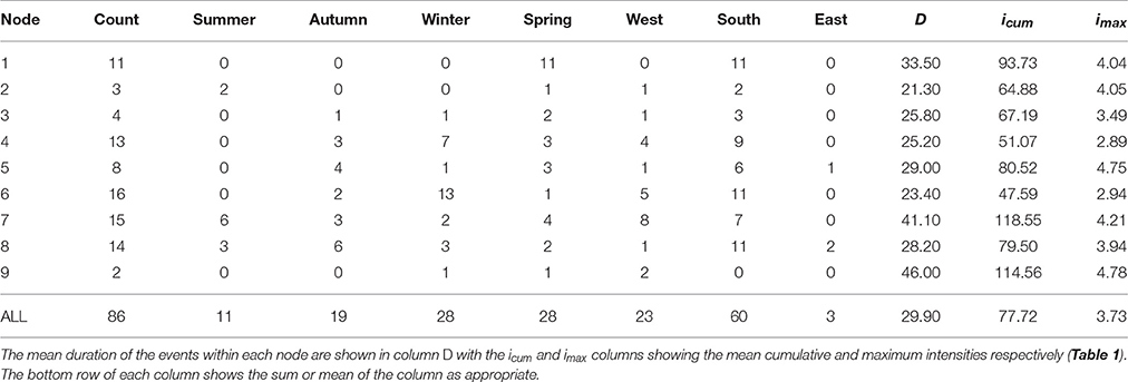
Table 2. The count of MHWs clustered into each node, count of events for each season, count of events for each coast, and relevant metrics for those MHWs.

Table 2 shows that the largest values for duration (D), cumulative intensity (i_cum) and maximum intensity (i_max) were more than twice those of the smallest values. An individual description of each node may be found below, with a qualitative summary of the patterns given in Table 3. It is important to note that the wind and current anomalies shown in Figure 4 do not show the absolute strength/direction of travel, but rather how these values deviated from the daily climatologies for the days during the MHWs in those nodes. The annual mean wind and current vectors may be seen in Figure 1.

TABLE 3

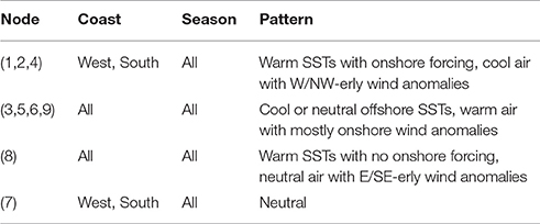
Table 3. Qualitative descriptions and groupings of the predominant atmospheric or oceanic patterns present across the SOM nodes.

3.2.1. Node 1

Node 1 showed the most striking oceanic pattern out of all of the nodes. The mean oceanic pattern from all of the MHW states clustered into this panel showed Agulhas Current leakage into the Atlantic as well as forcing onto the coastal region around the Cape Peninsula and potentially along the rest of the south coast. The SST anomalies along the coast, as well as in the open ocean were also the warmest of all the panels. The atmospheric temperature anomaly was mild relative to the other nodes but very strong north westerly wind anomalies were present to the west of the subcontinent and strong northerly wind anomalies to the east. The north-westerly wind anomalies continued to the south of the subcontinent and along the south coast up to the location of the occurrence of the most eastward MHW before encountering the Indian high and abating. Neither of the high pressure cells showed any real influence on the overland wind anomalies. Node 1 was unique in that all of the MHWs occurred during not only the same season (spring), but the same year (2004) as well. This also made it the node with highest concentration of spring events, as well as being one of only two nodes to have events that occurred on only one coast.

3.2.2. Node 2

Node 2 showed similar warm SST anomalies in the nearshore along the west and south coasts as Node 1, with open ocean anomalies being cooler. There appeared to be some onshore forcing and leakage of the Agulhas Current but it was not as strong as in Node 1. The atmospheric temperature and wind anomalies in this panel were slightly less than Node 1 as well. The wind anomaly patterns were shifted slightly more to the south west with the westerly wind anomalies along the bottom of the panel reaching further east. The anomalous offshore wind circulation did not appear to move onshore. The average duration of the events in this node were the shortest of all the nodes.

3.2.3. Node 3

Node 3 showed the most negative SST anomalies of all the nodes, with some warm SST anomalies still present along much of the three coasts. There were atypical surface currents occurring to the south west of the Cape Peninsula, similar to Nodes 1 and 2, but without clear onshore forcing. The overland atmospheric temperature anomalies were strong in this node with westerly wind anomalies pushing onshore along the west and south coasts from the south west and continuing overland. These onshore south-westerly anomalies were met on the eastern side of the subcontinent by neutral Indian high anomalies.

3.2.4. Node 4

Node 4 showed Agulhas leakage and onshore forcing with warm coastal SST anomalies along all three coasts, similar to Nodes 1 and 2. Warm open ocean SST and current anomalies were relatively even, with a large stretch of warmer SST anomalies and Agulhas retroflection along the bottom of the panel. Atmospheric temperature anomalies were relatively neutral, though slightly warmer over the subcontinent than the ocean. The wind anomalies were similar to Nodes 1 and 2, but with the largest westerly wind anomalies of all of the nodes. Of the 13 MHWs clustered into Node 4, 11 of them occurred during the same aseasonally warm year (2007), over a span of several months. The events in this node had, on average, the second shortest durations, second lowest cumulative intensities, and the lowest maximum intensities. This node therefore serves as a good representations of atmospheric and oceanic states during the smaller events in this study.

3.2.5. Node 5

Node 5 showed some atypical currents to the south west of the Cape Peninsula, similar to most of the nodes. The SST anomalies during the events in this node were a mix of warm and cold, with very mild warm anomalies present along most of the coast. The atmospheric temperature anomalies, particularly overland, were strong during these events. Even though the wind anomalies were slight over the ocean during the events in this node, they were stronger overland where anomalous onshore wind movement occurred. This is also one of only two nodes that contain an event that occurred on the east coast. The average maximum intensity for the events in this node is very nearly the greatest.

3.2.6. Node 6

The surface current and SST anomalies in Node 6 were very similar to Node 5, with fewer warm SST anomalies along the coast. The atmospheric temperature anomalies overland during these events were in excess of 7°C with strong south-easterly wind anomalies pushing not only onshore, but along the entire study area as well. The events clustered into this node had the greatest atmospheric temperature anomalies of all the nodes. Node 6 also shows a strong affinity for events from only one season, with 13 of the 16 MHW therein having occurred during winter, but were spread out from 1993 to 2014. This large concentration of winter events means that nearly half of all winter events were clustered into Node 6. The events in Node 4 battle those in Node 6 for the position of shortest and weakest, making this node another good example of the atmospheric and oceanic patterns during the smaller events used in this study. This node also has the greatest number of events clustered into it.

3.2.7. Node 7

Node 7 showed some atypical currents to the south west of the subcontinent but little in the way of onshore forcing or warm SST anomalies. The Southern Ocean appeared to be pushing up into the study area during these events as seen by the cold anomaly in the bottom middle of the panel. The atmospheric temperatures showed a very slight negative anomaly over much of the study area with very weak westerlies winds anomalies along the southern portion of the study area. That this node does not show any real patterns is not surprising given its position in relation to the nodes with stronger patterns. This node has the second greatest number of events clustered into it and contains half of all of the summer events in this study. These events also have the second longest average duration, the greatest average cumulative intensity, and the third greatest average maximum intensity. Because the node with the overall largest events only has two events clustered into it, Node 7 serves as the best representation of the atmospheric and oceanic patterns during very large events.

3.2.8. Node 8

Node 8 showed warm SST anomalies for all but the offshore portion of the Atlantic Ocean. There was some atypical vorticity along the south of the study area, but this was moving away from the coast and there appeared to be little leakage of the Agulhas Current. The atmospheric temperature anomalies during these events were small with strong easterly wind anomalies moving across the entire study area. These wind anomalies wrapped around the subcontinent, and were not found overland. This node contained two of the three events that occurred on the east coast, and the third highest total of events clustered into a single node.

3.2.9. Node 9

The final node showed cold SST anomalies along much of the south and west coasts, with some warm anomalies further south of the subcontinent and atypical vorticity to the south east that did not appear to be reaching the coast. Easterly wind anomalies were found along the bottom of the study area with warm atmospheric temperature anomalies throughout. There are some slight onshore wind anomalies along the entire coastline. This is the only node that contains events from only one location (site 1; Figure 1). The two events clustered into this node have between them the greatest duration and maximum intensity, with the second greatest cumulative intensity. This makes the events in this node the overall largest however, the low number of events clustered here prevent this node from being a good indicator of a common atmospheric or oceanic pattern.

4. Discussion

4.1. MHW States

The ordination of the MHW and climatology states has shown that they do differ in discernible ways. The clustering of the climatology states in the center of Figure 3 serves as a reference for better understanding the positioning of the MHW states. Because the proximity of points in an ordinated space shows their (dis)similarity to one another, the closer to the climatology states a MHW state may be found, the more it resembles it. This may seem contradictory at first given that all of the MHW states are ordinated most closely to climatology states that occurred during a different season. This means however that the states during all of the MHWs were aseasonal, and were more similar to climatology states during a different season of the year than the one in which they occurred. That none of the MHW states were ordinated near a winter climatology state is not surprising, as one would assume that MHWs should occur during warmer atmospheric or oceanic states. Following on this logic, a further assumption would be that the MHW states should most closely resemble the warmest time of year, summer. That the MHW states are instead ordinated more closely with autumn and spring climatology states means that high atmospheric or oceanic temperatures may be necessary for a MHW to occur, but are not the only driving force. During summer and winter months in southern Africa the Atlantic and Indian highs tend to stay in place latitudinally (Van Heerden and Hurry, 1998). It is during autumn and spring that, not always in a predictable manner, the synoptic atmospheric features around the subcontinent migrate north or south (Van Heerden and Hurry, 1998). As these systems shift they apparently create wind and/or current states that appear to be most similar to those that occurred during the coastal MHWs in this study. That high atmospheric and/or oceanic temperatures are not the only factor in the ordination of these MHW states is good as, under a warming global climate (Pachauri et al., 2014), this would likely mean an increase in MHWs. Instead we have found that it is aseasonality that is most consistently associated with MHW states. Therefore we may conclude that areas that experience increasingly divergent winds or currents from historical standards, without increasing temperatures, may also see an increase in MHWs.

Lastly, we have shown that in this ordinated space, the duration of the MHW around which each MHW state has been created, had a significant relationship with the proximity of the MHW state to climatology states. This is because the longer the event is, the more days of atmospheric and oceanic data are averaged together, creating a progressively smoother state, that will more closely resemble one of the climatology states. This is a potential, though unavoidable weakness in the methodology.

4.2. Agulhas Leakage

The most notable oceanic pattern from the clustering of these events into nodes with the use of a SOM has been Agulhas leakage. This phenomenon is when warm Indian Ocean water finds its way into the colder Atlantic Ocean (Beal et al., 2011). These warm eddies then typically spin up along the west coast. This transport of a large body of atypically warm water along a large stretch of coastline is a similar finding to the cause of the Western Australia MHW in 2011 where an unusual surge of the Leeuwin Current forced a large body of anomalously warm water onto the coast (Feng et al., 2013; Benthuysen et al., 2014). This onshore forcing of water is most apparent in Node 1 (Figure 4). However, Nodes 2 and 4 show a similar though less pronounced oceanic pattern, meaning that roughly one third of the events in this study occurred during Agulhas leakage. These three Agulhas leakage-dominated nodes also share the same anomalously warm atmospheric temperatures and north westerly to westerly wind anomaly patterns, to varying degrees. Therefore we may conclude that the predominant oceanic pattern during coastal MHWs is warm coastal SST anomalies occurring during Agulhas leakage while strong north-westerly wind anomalies exists along the west coast of the subcontinent, weak south-easterly wind anomalies along the east coast, and westerly wind anomalies that may be drawing aseasonally close to the south coast of the subcontinent. One of the primary causes of Agulhas leakage is when a weak Indian high does not provide enough of the positive wind stress curl the current needs to have enough inertia to retroflect upon meeting the Benguela current (Beal et al., 2011). The second feature that allows Agulhas leakage is when the latitude zero wind stress curl caused by the westerly wind belt has shifted further south of the subcontinent (Beal et al., 2011). We see in the Agulhas leakage panels that wind anomalies around the Indian high are much weaker than the Atlantic high. This could potentially be allowing for a loss in inertia of the Agulhas Current and an increased risk of leakage however, the westerlies appear to be shifted further north, which should inhibit leakage. These two diametric forces contributing to the atmospheric and oceanic states during the Agulhas leakage may be what is causing the Agulhas to move so close to the shore, leading to the large SST anomalies seen there.

Node 8 also shows some onshore forcing of the Agulhas Current, but with no large leakage into the Atlantic Ocean. Strong nearshore SST anomalies exist, but no ensuant leakage into the Atlantic due to the strong easterly wind anomalies over the Atlantic Ocean during the events in Node 8 that likely increased the inertia of the Agulhas Current enough that it retroflected upon meeting the Benguela current, while still forcing warm water onto the coast. Node 8 is also one of only two nodes that contain events from all three coasts, meaning that a strong Agulhas pushing onto the coast is a common pattern during MHW along the coastline of the entire study area.

Taken together with the events that occurred during Agulhas leakage, over half of the MHWs in this study occurred during some sort of anomalous Agulhas behavior coupled with warm nearshore SST anomalies. This is strong support for the relationship between the Agulhas Current and coastal MHWs. Beal et al. (2011) state, while difficult to say with certainty, Agulhas leakage is likely to increase under the continued regime of global anthropogenic warming. Biastoch et al. (2009) also found that Agulhas leakage is likely to increase, though due to the poleward shift of westerly winds. It is therefore likely that large MHWs like those seen in Nodes 1, 2, 4, and 8 will become more frequent.

4.3. Onshore Winds

With the exception of Nodes 7 and 8, all of the atmospheric states during coastal MHWs showed warm atmospheric temperature anomalies that were greater over the subcontinent than the ocean. The wind anomaly patterns during coastal MHWs were either strong north-westerly anomalies over the Atlantic with weak south-easterly anomalies over the Indian Ocean, or the inverse, but always showed some wind anomalies moving onshore. Furthermore, the nodes with the greatest overland atmospheric temperature anomalies (3, 5, 6, and 9) had comparable amounts of cold and warm SST anomalies as well as onshore wind anomalies. This implies that the MHWs in these nodes were forced by the onshore wind anomalies occurring during warm atmospheric anomalies and not by oceanic conditions. From this the conclusion may be drawn that MHWs forced by atmospheric variability will almost certainly occur during warm atmospheric anomalies with onshore wind anomalies. Three preferential mechanisms can be identified by which the pairing of atmospheric anomalies may cause MHWs. The first would be through direct atmospheric heating of the shallow nearshore water, as occurred over the Mediterranean in 2003 (Garrabou et al., 2009). The second could be that the anomalous onshore wind movement could have prevented seasonally regular wind forced upwelling from occurring, which would have then caused the coastal water at the location of the event to appear aseasonally warm. Lastly it is possible that the aseasonal wind anomalies could have acted upon the Agulhas Current, causing it to weaken and thereby broaden out over the Agulhas Bank and seeping warm water onto the cost. Taken together the events in these nodes (3, 5, 6, and 9) account for roughly one third of the events in this study.

4.4. Other Patterns

The lack of a strong atmospheric or oceanic pattern in Node 7 implies that the 15 events that were clustered there do not share any common pattern, meaning that there may still be many MHWs that occur not because of any recurrent or predominant atmospheric or oceanic pattern. This is an important finding as it shows that even though clear patterns in atmosphere and ocean may exist during most MHWs, these events may still occur during entirely novel conditions. A different interpretation of the lack of an apparent pattern in Node 7 is that because the events clustered into that event were the longest, on average, of all of the events in this study, creating a mean atmospheric and oceanic state for the entire duration of each event was impractical. That enough variation in atmosphere and ocean would have occurred over the lifespan of the event so as to “smooth out” any apparent signal. If this is so, it does not serve to address what may have caused such a large event. Upon closer inspection, the atlas figures for each event in Node 7 show that there are indeed patterns in the atmospheric and oceanic anomalies during these events, and that they do differ from the patterns in the other nodes.

The most seasonally predictable MHWs, those occurring during winter months and clustered into Node 6, were also the shortest and weakest. As these events were clearly a product of thermal heating, one could be led to assume that atmospheric forcing of MHWs causes less dramatic events than those forced by the ocean. This assumption would be incorrect as the MHWs clustered in Node 5, which also contain a clear atmospheric signal, have a greater cumulative intensity than most of the Agulhas leakage-dominated nodes. The largest events, those in Node 7, contain such disparate atmospheric and oceanic states that the mean atmospheric and oceanic patterns appear nearly blank. These factors prevent the drawing of a conclusion on whether the atmosphere or ocean may cause the largest MHWs.

A final note on the patterns visible in Figure 4. The south west corners of the oceanic states in Nodes 2, 3, 5, 6, 7, and 9, show an almost identical cyclonic (clockwise) anomaly on the exact same pixels. Upon more minute investigation it was determined that this cyclone, likely an Agulhas ring (Hutchings et al., 2009), occurred between roughly 12.5 to 14.5°E and 35.5 to 37.5°S. This eddy occurred during two thirds of all of the events in this study, making it the most common atmospheric or oceanic pattern found.

5. Conclusions

This research has shown that not only are the atmosphere and ocean states during coastal MHWs not closely related to the daily climatology states seen throughout the year, that what similarities do exist between MHW and climatology states are completely aseasonal. This means that the patterns that occur during MHW states are always more closely related to a different season than the one in which they occurred. Furthermore, the fewest MHWs occurred during summer months than any other season. These two facts taken together support the argument that MHWs are not simply a symptom of solar heating during the warm months of the year, but that aseasonal winds and/or currents are also necessary for a coastal MHW to occur. It is also possible that MHWs are recorded less frequently during summer months because coastal waters will be warmer, and incursions of offshore water, or atmospheric heating will not cause a large enough difference in the expected daily temperatures to be flagged as a MHW.

The predominant oceanic pattern that emerged from the SOM clustering of the MHW states was the abnormal advection of warm water onto the coast in association with Agulhas Current leakage. The predominant atmospheric state was anomalously warm air centered over the subcontinent coinciding with strong onshore wind anomalies. The node containing the most lengthy, cumulatively intense events lacked any patterns, meaning that the majority of the MHWs in this study that had the potential to cause the most harm to nearshore ecosystems do not appear to have consistent or recurrent atmospheric or oceanic states. Rather, most of the largest events occurred during a novel atmospheric and/or oceanic state that was not repeated often enough to receive their own node. A third smaller scale pattern was found to occur more frequently than both the predominant atmospheric and oceanic patterns detailed here. This was a sub-meso-scale anticyclonic eddy, roughly two degrees wide, and centered at 13.5°E and 36.5°S. We did not investigate the ocean dynamics implied by the presence of this eddy as that was beyond the scope of this study.

The methodology utilized here has shown that it is possible to discern predominant atmospheric and oceanic patterns that occur during MHWs; however, one must have knowledge of the meso-scale oceanic and atmospheric properties of the study area in order to correctly interrogate the results. Even with this knowledge, many of the largest MHWs did not show any relationship to these potential meso-scale forces. One must therefore not assume that such broad patterns in either the atmosphere or ocean must be forcing any single MHW observed in nearshore environments. We have however shown that the likelihood of a large coastal MHW is greater during specific atmospheric and oceanic patterns. Given this consideration, it should be possible to apply this methodology to large-scale reanalysis products in an effort to forecast the occurrence of coastal MHWs at a fine-scale.

In order to determine potential patterns that may or may not exist during MHWs, this study utilized atmospheric and oceanic surface temperatures and velocity vectors. This was done because of the few large MHWs whose causes have been discerned (e.g., Garrabou et al., 2009; Feng et al., 2013; Pearce and Feng, 2013; Benthuysen et al., 2014; Chen et al., 2015; Oliver et al., 2017a), most were related to these variables. Having shown that temperature and surface vorticity patterns do exist during coastal MHWs, a follow up to this study should analyse surface pressure, which was the main driver of the The Blob (Bond et al., 2015), as well as eddy kinetic energy (EKE), which was a primary driver of the 2015/16 Tasman Sea MHW (Oliver et al., 2017a).

Author Contributions

The central concept of developing a “Marine Heatwave Atlas” was first developed and implemented for Tasmania by EO with input from SP. RS then adapted this concept for use in South Africa. The idea to cluster recurrent atmospheric and oceanic states during marine heatwaves was also first implemented by EO with input from SP. The SACTN and ERA-Interim data were acquired by RS. The Aviso and OISST data were acquired by AS. All analyses, figures, and tables were performed or created by RS, with many of them adapted from earlier work performed by EO. All results were initially interpreted and drafted by RS, with EO, SP, AK, and AS providing two rounds of critical revisions on the developing manuscript. EO and AS provided additional insights into the oceanography of southern Africa while SP and AK provided additional insights into the meteorology. All authors give approval for the submission of this manuscript for review and agree to be accountable for all aspects of the work.

Funding

This research was supported by NRF Grant number CPRR14072378735 and ARC grant number DE140100952.

Conflict of Interest Statement

The authors declare that the research was conducted in the absence of any commercial or financial relationships that could be construed as a potential conflict of interest.

Acknowledgments

We would like to thank DAFF, DEA, EKZNW, KZNSB, SAWS, and SAEON for contributing all of the raw data used in this study. Without it, this article and the South African Coastal Temperature Network (SACTN) would not be possible. This paper makes a contribution to the objectives of the Australian Research Council Center of Excellence for Climate System Science (ARCCSS). The data and analyses used in this paper may be downloaded at https://github.com/schrob040/AHW. The metadata for each SACTN time series used in this study may be downloaded at https://github.com/schrob040/AHW/blob/master/setupParams/SACTN_site_list.csv.

Footnotes

1. ^https://robert-schlegel.shinyapps.io/SACTN/

2. ^https://github.com/ecjoliver/marineHeatWaves

References

Akinduko, A. A., Mirkes, E. M., and Gorban, A. N. (2016). SOM: Stochastic initialization versus principal components. Inf. Sci. 364–365, 213–221. doi: 10.1016/j.ins.2015.10.013

CrossRef Full Text | Google Scholar

Banzon, V., Smith, T. M., Chin, T. M., Liu, C., and Hankins, W. (2016). A long-term record of blended satellite and in situ sea-surface temperature for climate monitoring, modeling and environmental studies. Earth Syst. Sci. Data 8, 165–176. doi: 10.5194/essd-8-165-2016

CrossRef Full Text | Google Scholar

Beal, L. M., De Ruijter, W. P. M., Biastoch, A., Zahn, R., Cronin, M., Hermes, J., et al. (2011). On the role of the Agulhas system in ocean circulation and climate. Nature 472, 429–436. doi: 10.1038/nature09983

PubMed Abstract | CrossRef Full Text | Google Scholar

Benthuysen, J., Feng, M., and Zhong, L. (2014). Spatial patterns of warming off Western Australia during the 2011 Ningaloo Niño: quantifying impacts of remote and local forcing. Cont. Shelf Res. 91, 232–246. doi: 10.1016/j.csr.2014.09.014

CrossRef Full Text | Google Scholar

Biastoch, A., Böning, C. W., Schwarzkopf, F. U., Lutjeharms, J. R. E., Boning, C. W., Schwarzkopf, F. U., et al. (2009). Increase in Agulhas leakage due to poleward shift of Southern Hemisphere westerlies. Nature 462, 495–498. doi: 10.1038/nature08519

PubMed Abstract | CrossRef Full Text | Google Scholar

Bond, N. A., Cronin, M. F., Freeland, H., and Mantua, N. (2015). Causes and impacts of the 2014 warm anomaly in the NE Pacific. Geophys. Res. Lett. 42, 3414–3420. doi: 10.1002/2015GL063306

CrossRef Full Text | Google Scholar

Burrough, P. A., Wilson, J. P., Van Gaans, P. F. M., and Hansen, A. J. (2001). Fuzzy k-means classification of topo-climatic data as an aid to forest mapping in the Greater Yellowstone Area, USA. Landsc. Ecol. 16, 523–546. doi: 10.1023/A:1013167712622

CrossRef Full Text | Google Scholar

Castillo, K. D., and Lima, F. P. (2010). Comparison of in situ and satellite-derived (MODIS-Aqua/Terra) methods for assessing temperatures on coral reefs. Limnol. Oceanogr. Methods 8, 107–117. doi: 10.4319/lom.2010.8.0107

CrossRef Full Text | Google Scholar

Cavazos, T. (2000). Using self-organizing maps to investigate extreme climate events: An application to wintertime precipitation in the Balkans. J. Clim. 13, 1718–1732. doi: 10.1175/1520-0442(2000)013<1718:USOMTI>2.0.CO;2

CrossRef Full Text | Google Scholar

Cavole, L., Demko, A., Diner, R., Giddings, A., Koester, I., Pagniello, C., et al. (2016). Biological impacts of the 2013–2015 warm-water anomaly in the northeast pacific: winners, losers, and the future. Oceanography 29, 273–285. doi: 10.5670/oceanog.2016.32

CrossRef Full Text | Google Scholar

Chen, K., Gawarkiewicz, G., Kwon, Y.-O., and Zhang, W. G. (2015). The role of atmospheric forcing versus ocean advection during the extreme warming of the Northeast U.S. continental shelf in 2012. J. Geophys. Res. 120, 4324–4339. doi: 10.1002/2014JC010547

CrossRef Full Text | Google Scholar

Cooper, K. F. (2014). Evaluating Global Ocean Reanalysis Systems for the Greater Agulhas Current System. Masters Thesis, University of Cape Town.

Corte-Real, J., Qian, B., and Xu, H. (1998). Regional climate change in Portugal: precipitation variability associated with large-scale atmospheric circulation. Int. J. Climatol. 18, 619–635.

Google Scholar

Dee, D. P., Uppala, S. M., Simmons, A. J., Berrisford, P., Poli, P., Kobayashi, S., et al. (2011). The ERA-Interim reanalysis: configuration and performance of the data assimilation system. Q. J. R. Meteorol. Soc. 137, 553–597. doi: 10.1002/qj.828

CrossRef Full Text | Google Scholar

Feng, M., McPhaden, M. J., Xie, S.-P., and Hafner, J. (2013). La Niña forces unprecedented Leeuwin Current warming in 2011. Sci. Rep. 3:1277. doi: 10.1038/srep01277

PubMed Abstract | CrossRef Full Text | Google Scholar

Garrabou, J., Coma, R., Bensoussan, N., Bally, M., Chevaldonné, P., Cigliano, M., et al. (2009). Mass mortality in Northwestern Mediterranean rocky benthic communities: effects of the 2003 heat wave. Global Change Biol. 15, 1090–1103. doi: 10.1111/j.1365-2486.2008.01823.x

CrossRef Full Text | Google Scholar

Gibson, P. B., Perkins-Kirkpatrick, S. E., and Renwick, J. A. (2016). Projected changes in synoptic weather patterns over New Zealand examined through self-organizing maps. Int. J. Climatol. 36, 3934–3948. doi: 10.1002/joc.4604

CrossRef Full Text | Google Scholar

Hewitson, B. C., and Crane, R. G. (2002). Self-organizing maps: Applications to synoptic climatology. Clim. Res. 22, 13–26. doi: 10.3354/cr022013

CrossRef Full Text | Google Scholar

Hobday, A. J., Alexander, L. V., Perkins, S. E., Smale, D. A., Straub, S. C., Oliver, E. C., et al. (2016). A hierarchical approach to defining marine heatwaves. Progr. Oceanogr. 141, 227–238. doi: 10.1016/j.pocean.2015.12.014

CrossRef Full Text | Google Scholar

Hutchings, L., van der Lingen, C. D., Shannon, L. J., Crawford, R. J. M., Verheye, H. M. S., Bartholomae, C. H., et al. (2009). The Benguela Current: an ecosystem of four components. Progr. Oceanogr. 83, 15–32. doi: 10.1016/j.pocean.2009.07.046

CrossRef Full Text | Google Scholar

Jain, A. K. (2010). Data clustering: 50 years beyond K-means. Pattern Recogn. Lett. 31, 651–666. doi: 10.1016/j.patrec.2009.09.011

CrossRef Full Text | Google Scholar

Johnson, N. C. (2013). How many enso flavors can we distinguish? J. Clim. 26, 4816–4827. doi: 10.1175/JCLI-D-12-00649.1

CrossRef Full Text | Google Scholar

Kruskal, J. B. (1964). Nonmetric multidimensional scaling: a numerical method. Psychometrika 29, 115–129. doi: 10.1007/BF02289694

CrossRef Full Text | Google Scholar

Kumar, J., Mills, R. T., Hoffman, F. M., and Hargrove, W. W. (2011). Parallel k-means clustering for quantitative ecoregion delineation using large data sets. Proc. Comput. Sci. 4, 1602–1611. doi: 10.1016/j.procs.2011.04.173

CrossRef Full Text | Google Scholar

Lünning, K. (1990). Seaweds: Their Environment, Biogeography and Ecophysiology. New York, NY: Wiley.

Google Scholar

Lutjeharms, J., Cooper, J., and Roberts, M. (2000). Upwelling at the inshore edge of the Agulhas Current. Cont. Shelf Res. 20, 737–761. doi: 10.1016/S0278-4343(99)00092-8

CrossRef Full Text | Google Scholar

Mills, K., Pershing, A., Brown, C., Chen, Y., Chiang, F.-S., Holland, D., et al. (2013). Fisheries management in a changing climate: lessons from the 2012 ocean heat wave in the Northwest Atlantic. Oceanography 26, 191–195. doi: 10.5670/oceanog.2013.27

CrossRef Full Text | Google Scholar

Minchin, P. R. (1987). An evaluation of the relative robustness of techniques for ecological ordination. Vegetatio 69, 89–107. doi: 10.1007/BF00038690

CrossRef Full Text | Google Scholar

Morioka, Y., Tozuka, T., and Yamagata, T. (2010). Climate variability in the southern Indian Ocean as revealed by self-organizing maps. Clim. Dynamics 35, 1075–1088. doi: 10.1007/s00382-010-0843-x

CrossRef Full Text | Google Scholar

Oksanen, J., Blanchet, F. G., Friendly, M., Kindt, R., Legendre, P., McGlinn, D., et al. (2017). Vegan: Community Ecology Package. Oulu.

Google Scholar

Oliver, E. C. J., Benthuysen, J. A., Bindoff, N. L., Hobday, A. J., Holbrook, N. J., Mundy, C. N., et al. (2017a). The unprecedented 2015/16 Tasman Sea marine heatwave. Nat. Commun. 8:16101. doi: 10.1038/ncomms16101

PubMed Abstract | CrossRef Full Text | Google Scholar

Oliver, E. C. J., Lago, V., Holbrook, N. J., Ling, S. D., Mundy, C. N., and Hobday, A. J. (2017b). Eastern Tasmania Marine Heatwave Atlas. Hobart: University of Tasmania.

Pachauri, R. K., Allen, M. R., Barros, V. R., Broome, J., Cramer, W., Christ, R., et al. (2014). Climate Change 2014: Synthesis Report. Contribution of Working Groups I, II and III to the Fifth Assessment Report of the Intergovernmental Panel on Climate Change. Geneva: IPCC.

Google Scholar

Paliy, O., and Shankar, V. (2016). Application of multivariate statistical techniques in microbial ecology. Mol. Ecol. 25, 1032–1057. doi: 10.1111/mec.13536

PubMed Abstract | CrossRef Full Text | Google Scholar

Pearce, A. F., and Feng, M. (2013). The rise and fall of the “marine heat wave” off Western Australia during the summer of 2010/2011. J. Mar. Syst. 111–112, 139–156. doi: 10.1016/j.jmarsys.2012.10.009

CrossRef Full Text | Google Scholar

Perkins, S. E., and Alexander, L. V. (2013). On the measurement of heat waves. J. Clim. 26, 4500–4517. doi: 10.1175/JCLI-D-12-00383.1

CrossRef Full Text | Google Scholar

Rossi, F. (2012). Yasomi: Yet Another Self Organising Map Implementation. Paris.

Schlegel, R. W., Oliver, E. C. J., Wernberg, T., and Smit, A. J. (2017). Nearshore and offshore co-occurrence of marine heatwaves and cold-spells. Progr. Oceanogr. 151, 189–205. doi: 10.1016/j.pocean.2017.01.004

CrossRef Full Text | Google Scholar

Schlegel, R. W., and Smit, A. J. (2016). Climate Change in Coastal Waters: Time Series Properties Affecting Trend Estimation. J. Clim. 29, 9113–9124. doi: 10.1175/JCLI-D-16-0014.1

CrossRef Full Text | Google Scholar

Smale, D. A., and Wernberg, T. (2009). Satellite-derived SST data as a proxy for water temperature in nearshore benthic ecology Peer reviewed article. Mar. Biol. 387, 27–37. doi: 10.3354/meps08132

CrossRef Full Text | Google Scholar

Smit, A. J., Oliver, E. C. J., and Schlegel, R. W. (2017). RmarineHeatWaves: Package for the Calculation of Marine Heat Waves. University of the Western Cape, Belville.

Smit, A. J., Roberts, M., Anderson, R. J., Dufois, F., Dudley, S. F. J., Bornman, T. G., et al. (2013). A coastal seawater temperature dataset for biogeographical studies: large biases between in situ and remotely-sensed data sets around the coast of South Africa. PLOS ONE 8:0081944. doi: 10.1371/journal.pone.0081944.

PubMed Abstract | CrossRef Full Text | Google Scholar

Stachowicz, J. J., Terwin, J. R., Whitlatch, R. B., and Osman, R. W. (2002). Linking climate change and biological invasions: ocean warming facilitates nonindigenous species invasions. Proc. Natl. Acad. Sci. U.S.A. 99, 15497–15500. doi: 10.1073/pnas.242437499

PubMed Abstract | CrossRef Full Text | Google Scholar

Tyson, P. D., and Preston-Whyte, R. A. (2000). Weather and Climate of Southern Africa. Cape Town: Oxford University Press.

Google Scholar

Unal, Y., Kindap, T., and Karaca, M. (2003). Redefining the climate zones of Turkey using cluster analysis. Int. J. Climatol. 23, 1045–1055. doi: 10.1002/joc.910

CrossRef Full Text | Google Scholar

Van Heerden, J., and Hurry, L. (1998). Southern Africa's Weather Patterns: An Introductory Guide. Pretoria: Collegium.

Wernberg, T., Bennett, S., Babcock, R. C., Bettignies, T. D., Cure, K., Depczynski, M., et al. (2016). Climate driven regime shift of a temperate marine ecosystem. Science 149, 2009–2012. doi: 10.1126/science.aad8745

CrossRef Full Text | Google Scholar

Wernberg, T., Russell, B. D., Moore, P. J., Ling, S. D., Smale, D. A., Campbell, A., et al. (2011). Impacts of climate change in a global hotspot for temperate marine biodiversity and ocean warming. J. Exp. Mar. Biol. Ecol. 400, 7–16. doi: 10.1016/j.jembe.2011.02.021

CrossRef Full Text | Google Scholar