Ocean Futures Under Ocean Acidification, Marine Protection, and Changing Fishing Pressures Explored Using a Worldwide Suite of Ecosystem Models

Introduction

The world's oceans are facing the effects of globalization and a growing human population through increasing anthropogenic pressures, ranging from acidification (Barange et al., 2010) to increased use of ecosystem services and resources [e.g., renewable energy (Plummer and Feist, 2016), petroleum extraction (Marshak et al., 2017), fisheries (Pauly and Zeller, 2016), and aquaculture (Belton et al., 2016)]. In response, there is an ever louder call for increased protection of the oceans (McCauley et al., 2015; Hilborn, 2016). Status reports on fishery resources are mixed; many effectively managed fisheries are rebuilding or rebuilt (Hilborn and Ovando, 2014), while many unmanaged or ineffectively managed fisheries are declining and potentially overfished (Pikitch, 2012; Halpern et al., 2015; Bundy et al., 2016).

The effort to strategically manage natural resources in a holistic and integrative context, where tradeoffs for the ecosystem service needs of multiple use sectors are considered, is commonly referred to as ecosystem-based management (EBM; Link, 2010; Ihde and Townsend, 2013). Challenges and proposed solutions to balancing sustainable ocean use and conservation form part of the canvas of twenty first century EBM. At the heart of EBM lies the need to better understand and predict interactions between ecosystem components, as well as to evaluate the consequences of possible futures and proposed management actions on the whole ecosystem. New tools need to be adapted and applied for EBM to be fully realized.

End-to-end marine ecosystem models can include the dynamics of the entire ecosystem from physics to human users (Plaganyi, 2007). With various levels of complexity, these models provide a useful platform for exploring the effects of management options (Kaplan et al., 2012; Fulton et al., 2014). Atlantis (Fulton et al., 2004a, 2011), a three-dimensional, spatially-explicit end-to-end ecosystem model, has seen worldwide application (currently 30 extant models, Weijerman et al., 2016b) since its development in the early 2000s (Fulton et al., 2011). Atlantis modeling does not attempt to find a single “optimal” management strategy, since there are often conflicting goals between conservation and extraction, but can quantitatively evaluate the socio-ecological tradeoffs of alternative management scenarios, functioning as an important decision-support tool.

Previous modeling case studies (Kaplan et al., 2012; Fulton et al., 2014), supported by field studies (Leslie et al., 2015), illustrate that no “silver bullet” EBM solution exists and that as humans continue to place increasing demands on the ocean we must expect tradeoffs among objectives (Link, 2010). At a strategic decision making level (i.e., 10+ year planning horizon that is of particular importance for sectoral EBM), case studies ranging from the USA West Coast to Antarctica (Kaplan et al., 2012; Weijerman et al., 2016b; Holsman et al., 2017; Longo et al., 2017), together with discussions of the main drivers influencing future state of the extant Atlantis ecosystem models, suggest that tradeoffs are particularly evident for the three following sets of scenarios in fisheries management:

Anticipating Effects of Ocean Acidification

The decrease in ocean pH resulting from accumulated atmospheric CO₂ dissolving into seawater (i.e., ocean acidification) will change ocean conditions for calcifying organisms such as mollusks, corals, and some plankton, negatively affecting survival, calcification, growth, development, and abundance (Kroeker et al., 2013; Browman, 2016). Ocean acidification is expected to have profound direct ecological and economic impacts on these calcifying organisms (Cooley and Doney, 2009) and some non-calcifying species that are sensitive to water chemistry (Busch and McElhany, 2016). However, it remains unclear to what extent there will be indirect repercussions through the food web for higher-trophic level species and for a broader set of fisheries. Case studies suggest that ocean acidification will lead to a decline in prey that subsequently impacts higher trophic levels, but these case studies lack a global perspective as well as a consistent interpretation of the direct effects of pH. For example, early food web modeling by Ainsworth et al. (2011a) based on Ecosim (Christensen and Walters, 2004) food-web models for the Northeast Pacific suggested effects of ocean acidification on higher-trophic level biomass and harvests; effects were often weak, but were evident in both benthic and pelagic predators. In contrast to this, Atlantis modeling of the California Current (Kaplan et al., 2010; Marshall et al., 2017) and SE Australia (Griffith et al., 2011, 2012) found stronger impacts on some benthic species such as flatfish and elasmobranchs, while a similar Atlantis modeling study of the NE USA (Fay et al., 2017) found both direct and indirect ecosystem effects. More recently, syntheses of experimental literature related to 300+ laboratory and field studies (Kroeker et al., 2013; Busch and McElhany, 2016) have provided insight about which species are most likely directly vulnerable to ocean acidification. Here we take a broad, global view (rather than case study specific) to explore the likely indirect (trophic) effects of ocean acidification, by applying lessons learned from the newly synthesized laboratory and field studies.

Implementation of Marine Protected Areas

Marine protected areas (MPAs) that are designed to exclude or limit some types of fishing and other activities (Halpern et al., 2010) may increase organism density, size, biomass, and spillover into adjacent areas (Lester et al., 2009; Gill et al., 2017). MPAs can be effective tools to achieve conservation and fisheries management objectives, but questions exist regarding the extent to which these gains may be uneven across species and whether conservation costs may be borne by fisheries. Differential effects on species may be expected; for instance, in a global meta-analysis of MPAs Lester et al. (2009) found that both fish and invertebrates increase in abundance in MPAs, but that invertebrates such as mollusks and arthropods benefit the most. This is consistent with a global meta-analysis that identified strong impacts of bottom fishing gears on these benthic taxa and their habitat (Kaiser et al., 2006). Lester et al. (2009) found that higher-trophic level species, which are often directly harvested, also exhibit strong increases in MPAs, and temperate systems respond similarly or even slightly more strongly than tropical systems to protection measures. In an evaluation of modeling studies of MPAs, Fulton et al. (2015) found that although MPAs can have positive economic benefits, the relationship between fishery yield and MPA area is non-linear and complex. Similarly, if MPAs are too large, economic benefits may be diminished. Unintended effects such as displaced effort or trophic cascades have been suggested by many modeling studies of MPAs, for instance by Walters et al. (1999), and more recently by Savina et al. (2013) who found negative impacts on prey fish when MPAs promoted shark recovery in a study of New South Wales, Australia. Here we test the assertion by Fulton et al. (2015) that MPAs perform best in terms of specific objectives related to species recovery, but that they can lead to tradeoffs across species and ecological objectives such as biodiversity and economic equity.

Planning the Mix or Balance of Fishing Effort across Species

Future fishery management across the globe will likely involve a new mix of fisheries (i.e., gears and target species), either in a proactive attempt to address inherent ecological effects on fish population productivity or simply due to worldwide trends that suggest declining or stable global industrial and demersal catches, while artisanal harvests and harvests of pelagic stocks and invertebrates continue to increase (Link et al., 2009; Worm et al., 2009; Pauly and Zeller, 2016). Previous ecological modeling results suggest that fish populations are mutually dependent upon one another (via competition and predation) and hence affect each other's productivity (Walters et al., 2005; Link et al., 2011; Voss et al., 2014). For instance, system level maximum sustainable yield (MSY) may be less than the sum of the individual species MSYs (May et al., 1979; Link et al., 2012) because assessed predator populations are less productive than would be predicted with traditional single-species management approaches if their prey are also being fished. Although fisheries policies in most nations do not address this interconnected nature of fish populations, (Garcia et al., 2012; Skern-Mauritzen et al., 2016) and subsequent modeling studies (Jacobsen et al., 2014) suggest fisheries should start addressing multispecies selectivity and targeting in a way that explicitly addresses interconnectedness. Achieving sustainable multispecies harvesting could begin with incremental adjustments of individual fishery sectors that move toward harvest rates that do account for differential productivity, vulnerability, and ecosystem roles across multiple trophic levels (Worm et al., 2009). Here we test how effects on ecosystem structure vary when we consider strong increases (or decreases) in effort by particular fishing sectors, and contrast this to results from base case scenarios that continue fishing patterns from the present day or recent past (Table 1).

TABLE 1

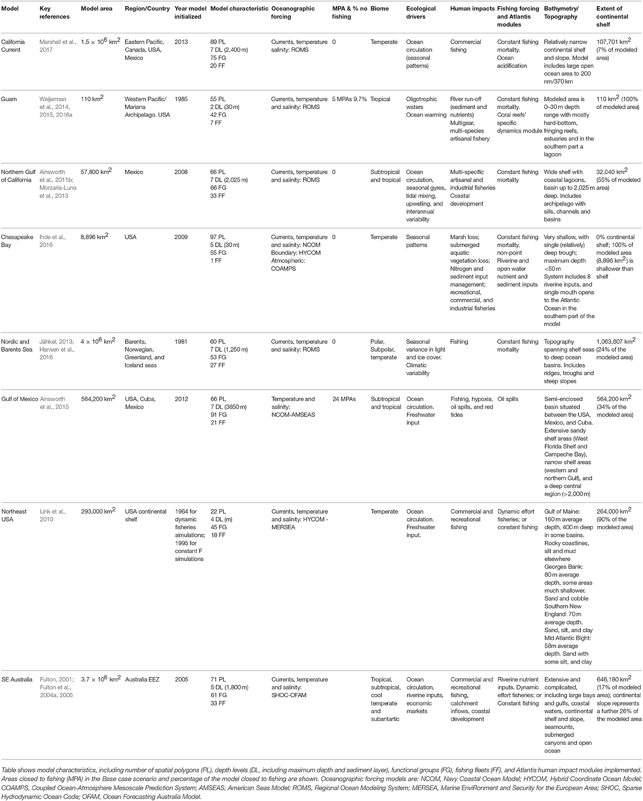
Table 1. Atlantis ecosystem models used in simulations.

A comparative approach (Megrey et al., 2009c; Murawski et al., 2010) is at the basis of our study; past efforts comparing empirical and scenario results across a range of ecosystems have proven to be an effective way to understand dynamics and potential impacts of perturbations when direct experimentation is not possible (e.g., Drinkwater et al., 2009; Gaichas et al., 2009; Link et al., 2009; Megrey et al., 2009a; Mueter et al., 2009; Bundy et al., 2012; Fu et al., 2012; Holsman et al., 2012). Our common modeling framework is more complex than in, e.g., Link et al. (2012), allowing us to examine additional interactions between the environment, living marine resources, and management. Here, we test whether EBM tradeoffs within the three sets of scenarios described above are consistent across a global suite of ecosystems, as represented by Atlantis models that vary in climate, spatial footprint, and ecological focus (Table 1, Figure 1). As the scenarios are a combination of external drivers (ocean acidification) and human activities and management actions (fisheries and marine protection) our analysis provides a high-level global analysis of the trade-offs between various levels of protection and human use under different levels of ocean acidification. Such trade-offs are particularly valuable in the current time when our planet is facing the effects of climate change with a growing population needing protein sources while upholding the health and biodiversity of the planet's marine ecosystems.

FIGURE 1

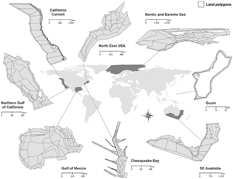
Figure 1. Atlantis ecosystem model domains (see Table 1 for model details).

As detailed in the Methods for each scenario, we investigated (1) increasing mortality due to ocean acidification, applying direct additional mortality to species identified as vulnerable in a global meta-analysis (Kroeker et al., 2013), at rates of 1% day⁻¹ and 0.5% day⁻¹ (consistent with prior modeling studies, Kaplan et al., 2010; Fay et al., 2017); (2) increasingly larger MPAs, closing 10, 25, or 50% of continental shelf waters <250 m deep; and (3) adjustments of individual fishery sectors that move toward accounting for differential productivity, vulnerability, and ecosystem roles across multiple trophic levels. This included tests doubling, halving, or eliminating fishing rates on small pelagic fish, invertebrates, and demersal fish. These scenarios were applied to eight extant Atlantis models in a common manner, projected for 50 years, and compared to a base-case simulating a continuation of status quo management with no changes in acidification or any aspect of fisheries management. Through these scenarios, we were able to explore tradeoffs related to pressures on ecosystems ranging from the arctic to the tropics, coastal to oceanic, and spanning both hemispheres. The multiple models were developed under a range of circumstances, but we took the approach of using the status quo system state as the base state in each case and then modifying from there. In this way, we show the differential system benefits (or impacts) to the different locations of potential future changes. We recognize that differences in the status quo or base case mean that some measures (e.g., introduction of MPAs) may not have as large an effect in some locations (e.g., Australia, which already has extensive spatial management in place) as in others. Nonetheless, we can give immediately relevant advice to the respective management agencies in the different locations (many of whom collaborate with the model builders, so direct relevance is important).

Materials and Methods

We used eight ecosystem models built in the end-to-end Atlantis framework to simulate common scenarios. These models represent marine ecosystems spanning a range of climates, sizes, and ecological characteristics (Table 1) across both hemispheres (Figure 1):

1. The California Current ecosystem is an eastern boundary current, dominated by episodic upwelling that drives biological productivity. Sardine and anchovy in particular demonstrate decade-long cycles. Fisheries include industrial and small-scale fisheries, with high landings of Pacific hake (Merluccius productus), sardine (Sardinops sagax), and squid (Doryteuthis opalescens), and high landed value of Dungeness crab (Metacarcinus magister). With the exception of salmon (Oncorhynchus spp.), most stocks are above fishery reference points, including most rockfish (Sebastes) species that have recovered from past overfishing.

2. The Guam ecosystem model focusses on the shallow (<30 m) coral reef ecosystem that surrounds the island. Despite being situated in oligotrophic waters, it is highly productive and supports multi-gear, multi-species coral reef fisheries, with a commercial and, most importantly, a recreation/cultural component. In the last decades reef fish biomass has declined substantially despite the establishment of five marine protected areas that are currently in place.

3. The Northern Gulf of California spans subtropical and tropical climate zones and is dominated by ocean circulation (including seasonal gyres), tidal mixing, upwelling, and interannual variability (i.e., ENSO, El Niño-Southern Oscillation). This region has a high primary productivity and is biodiverse. Fisheries include shrimp trawlers and industrialized purse seine vessels (in the south), but small-scale fisheries targeting over 80 species dominate in terms of the number of boats operating and fishers employed (Cinti et al., 2010). Overfishing is a major issue due to the lack of regulations and insufficient monitoring and enforcement of existing regulations (Páez-Osuna et al., 2017).

4. Chesapeake Bay is the largest estuarine embayment in the USA. The system is heavily impacted by nutrient enrichment due to a large coastal population (more than 17 million) and agricultural runoff of the large watershed (more than 165,000 km²) encompassing portions of 6 states. Though highly productive, the system is subject to annual and large hypoxic events resulting from over-enrichment. Fisheries are diverse (both in target species and gears employed), owing to the large number of transient species throughout the year in this system. However, the main fisheries target blue crab (Callinectes sapidus), striped bass (Morone saxatilis), Atlantic menhaden (Brevoortia tyrannus), and eastern oyster (Crassostrea virginica). Both recreational and commercial fisheries are important in the Chesapeake system. Individual commercial fisheries are comprised of mainly small operations of one or a few fishers often working from a single, relatively small vessel. The commercial menhaden fishery is the exception, with the lower Chesapeake Bay seeing large harvests of this forage fish. Even so, exploitation levels are generally modest, in part, because many of the species here are migratory, and those fish in the system are often small or in juvenile stages, using the estuary as a nursery. In contrast, the eastern oyster, a historically-crucial species for habitat production, is heavily harvested, but it remains unassessed. Estimates suggest that less than one percent of the virgin population of oyster remains (Newell, 1988; Wilberg and Miller, 2010), due to a combination of exploitation and disease.

5. The Nordic and Barents seas are shelf and deep-sea ecosystems with high seasonal productivity in the summer due to the inflow of nutrients and deep mixing followed by stratification. The current system is dominated by the Norwegian Atlantic slope current (Orvik and Skagset, 2005), which transports heat northwards into the Barents Sea and Polar ocean. There are strong fronts between the warm, saline waters and the polar and sub-polar water masses in the area. The system supports large pelagic and demersal fisheries that are currently sustainably managed, with the exception of a few species like Golden redfish (Sebastes marinus) and coastal cod (Gadus morhua). Precautionary managed fish stocks and good recruitment conditions over the last decades (Kjesbu et al., 2014) have contributed together to the current status of healthy stocks and sound management.

6. The Gulf of Mexico spans subtropical and tropical climates and is driven by circulation of the Loop Current and freshwater input. This region encompasses some of the most productive ecosystems in North America, while it is impacted by a variety of anthropogenic disturbances including fishing, hypoxia, oil production, and red tides. Commercial fishing includes purse seine, pelagic longline, and other hook-and-line gear, trawls, traps, and dredges, and recreational and for-hire (charter) fishing is an important economic sector for USA ports. Though fishing has been reduced in recent decades, roughly 1/5 of stocks are in a depleted (“overfished”) state (Karnauskas et al., 2017).

7. Northeast USA (NEUS) is a diverse and highly productive ecosystem (~350–400 g C m⁻² yr⁻¹), confined almost entirely to the continental shelf which has supported numerous significant commercial fisheries for centuries. Because the modeled ecosystem is large (extending from the Gulf of Maine to Cape Hatteras, NC), there are regional differences. The Gulf of Maine is a large marine basin with lower productivity, except in the Northwest coastal area, than in the rest of the NEUS Large Marine Ecosystem (LME). Georges Bank is a relatively large, shallow, submerged marine plateau with very high annual productivity. The Southern New England and Mid Atlantic Bight make up the rest of the NEUS LME with high productivity in nearshore regions. Benthic invertebrate fisheries are currently the most valuable in Georges Bank and the Gulf of Maine, but demersal and pelagic fisheries are active throughout the entire NEUS LME. Many demersal groundfish species are overexploited to collapsed in Gulf of Maine and Georges Bank but small pelagics are at high population levels.

8. Southeast Australia covers 3.7 million km² of Australia's southeastern EEZ, extending from the shoreline out into the open ocean and from tropical/subtropical waters of southern Queensland to cool temperate and subantarctic environments off southern Tasmania. The two poleward flowing currents that dominate the area lead to low relative primary productivity (compared to the other systems modeled here), but is one of the fastest warming marine areas on the globe (Wu et al., 2012). The fisheries in the region have been rebuilt over the last decade and the latest status reports indicate that while a few overfished species are still recovering, overfishing in the area has ceased (Patterson et al., 2017).

We simulated three common EBM questions: (1) Increasing ocean acidification: the increase in ocean pH resulting from accumulated atmospheric CO₂ dissolving into seawater (i.e., ocean acidification) will change ocean conditions for calcifying organisms, like mollusks and corals (Kroeker et al., 2013). Ocean acidification is expected to have profound ecological and economic impacts on calcifying organisms (Ocean Conservancy et al., 2015). (2) Increasing marine protection leading to increasingly larger areas closed to fishing: closing regions of the ocean to fisheries (i.e., MPAs) may increase fish density, size, biomass, and spillover into adjacent areas; thus MPAs serve as effective EBM, conservation, and fisheries management tools (Weigel et al., 2014). (3) Changes in fishing pressure: gradients of fishing effort may alter ecosystem functioning, including structural and functional components, and may serve as performance measures for fisheries management (Henriques et al., 2014). Below we detail the Atlantis ecosystem model framework, the parameterized marine ecosystems investigated, and the common-scenarios tested.

Atlantis Ecosystem Modeling Framework

Atlantis represents physical oceanography, nutrient cycling, trophic dynamics from primary producers to apex predators, and fisheries in a three-dimensional, spatially-explicit domain (Fulton et al., 2004a,b, 2011). The complexity of Atlantis facilitates region-specific parameterization of each ecosystem model, leading to the simulation of realistic current ecosystem dynamics and spatially-explicit predictions of future dynamics. Furthermore, Atlantis allows for two-way coupling between ecosystem components and human sectors, making it possible to examine ecosystem and human responses to combinations of environmental and anthropogenic pressures (Fulton, 2011). Simulated futures produced by Atlantis models include trophic and spatial dynamics allowing the prediction of indirect trophic effects on species that may not be directly impacted by anthropogenic pressures (Nye et al., 2013).

The technical specifications of the Atlantis framework, including process equations, can be found in Fulton (2001) and Fulton et al. (2004a,b, 2011). Further information can also be found on the Atlantis wiki¹ and published model applications (i.e., Smith et al., 2015; Nyamweya et al., 2016). Briefly, the Atlantis code base is structured in submodels that can be selectively implemented, including ecology, fisheries, monitoring, assessment, and management. Atlantis solves a system of forward differential equations that simulate ecosystem processes typically on a 12-h time-step. Modeled regions are represented in a 3D structure of horizontal polygons and vertical depth layers that match the biogeographical features of the marine system. The biological components of the system are represented by single- or multi-species functional groups, based on model objectives. Nutrient flow in Atlantis is simulated explicitly through the major food web components. Primary production is nutrient-, light-, space-, and temperature- dependent. Lower trophic levels are modeled as biomass pools and vertebrates (and in some cases key exploited invertebrates) are modeled as age-structured stocks. Multiple alternative formulations are available for ecological processes, according to the desired complexity; these processes are replicated in each polygon and depth layer. Atlantis models may include a detailed representation of human impacts (i.e., oil extraction or human development), fishing fleet characteristics such as target species, gear, and fishing location, and management boundaries including MPAs.

Common Scenarios

Simulations were projected forward for 50 years from the initialization year (Table 1). The scenarios simulated by each model depended on model characteristics and parameterization (Table 1, Table S1). For the SE Australia model (Fulton et al., 2005) and the NE USA model (Link et al., 2010), two different model versions were used, one that applies constant fishing and one that uses dynamic fishing effort. These models are identical in other parameters and configuration, but are reported separately in the results.

The scenarios simulated were:

1. Base case: Represents business as usual for each ecosystem model and served as the reference to which all other scenarios were compared. Parameterization of each base-case scenario was set to the calibrated, published parameter values, and therefore, each ecosystem in the base-case scenario may assume different current conditions, which reflect realistic differences in the ecology, fisheries, and management of the eight ecosystems. Additionally, future conditions including climate change are set for each model depending on assumptions in the published, calibrated parameterization. Fishing was assumed to continue at the constant rate used to calibrate each model. If nutrient dynamics were included in the calibrated ecosystem, then future nutrient conditions were assumed to follow the most recent average annual cycle.

2. Ocean acidification (OA): We tested two scenarios of additional mortality (day⁻¹) of 0.5 and 1%, added to the base-case natural mortality rates of calcifying algae, corals, coccolithophores, echinoderms, and mollusks. These increased rates simulated effects of ocean acidification on survival, roughly following the results from a global meta-analysis (Kroeker et al., 2013). These rates of 1 and 0.5% (day⁻¹) are consistent with other simulation case studies (Kaplan et al., 2010; Fay et al., 2017), and intentionally lead to strong declines in directly affected groups despite their relatively high productivity. Functional groups affected in each model are shown in the supporting information. We simulated ocean acidification scenarios with all eight ecosystems, including constant fishing and dynamic fishing effort versions for the SE Australia model and the NE USA model (total of 10 models).

3. Spatial management: Three hypothetical no-take MPA scenarios were used to evaluate the effect of MPA size on future ecosystem conditions. MPAs were extended from shore to deeper areas until 10, 25, and 50% of the continental shelf was closed to all fishing (i.e., recreational and commercial). MPAs were only implemented in the continental shelf area of each ecosystem, where the continental shelf was defined as all areas shallower than 250 m. Fishing rates in areas outside of the MPA were maintained at the fishing mortality rates in the base case. Therefore, MPA scenarios represent the case where fishing effort is removed rather than displaced. Total model area closed in each spatial management scenario is shown in Table S1. We simulated the scenarios with all eight models, including constant fishing and dynamic fishing effort versions for the SE Australia model.

4. Fisheries management: Fishing mortality rates (F) on species fished in the base-case scenario were doubled, halved, and eliminated, leading to three additional scenarios per model. Seven models were used to test these scenarios (excluding the Nordic and Barents Sea model, because it only included fisheries calculated to maximum sustainable yield, not historical levels). For the NE USA and SE Australia models, we applied the constant fishing version rather than the dynamic fishing version for these simple scenarios. Compared to more pelagic systems, the Guam coral reef model did not have the same “large” pelagic species and no highly migratory species, so scenario 4e (below) was not modeled for Guam.

Base fishing mortality rates and taxa included in each scenario are shown in the supporting information. Scenarios for fisheries management were applied to:

a. All Harvested Taxa

b. All Harvested Invertebrates

c. All Harvested Small pelagic fish

d. All Harvested Demersal fish and sharks

e. All Harvested Large pelagic and Highly migratory species

We report results from the full set of fisheries management scenarios in the Supplemental Information, but in the main text focus on doubling fishing mortality rates for Small pelagic fish or Invertebrates, and halving fishing mortality rates for Demersal fish and sharks, as framed in the Introduction.

In all scenarios other than the base case, drivers (e.g., ocean acidification mortality, or doubled fishing mortality) were applied in year 1 and held constant through the simulation. In our analysis this allows comparison of the simulations under the same time horizon, but is admittedly a crude simplification of reality. For instance, in reality, ocean acidification is a gradual change happening over years or even decades, while changes in fisheries management and changes in marine protection are typically instantaneous events resulting from management actions - although they may still take time to play out due to system interactions or because of rules built into harvest control rules, which often contain stability rules setting maximum rates of change in quotas to aid economic stability for the fishing sector. The authors are keenly aware that the interaction between the OA, MPA, and fisheries scenarios are often of particular interest (given the complex reality facing fisheries managers). Unfortunately, it was not possible to consider such interactions in this instance as such combinatoric analyses quickly become time and computationally intensive and would have increased the complexity of the analysis beyond the resources currently available to the authors.

Analysis

Comparisons: Biomass

We report results under each scenario as biomass response of individual functional groups and ecological indicators, described below. We focus the results on functional group biomass at the end of the simulations, averaged over simulation years 45–50, to integrate over any inter-annual variability driven by oceanography. We report biomass in each scenario relative to biomass averaged over years 45–50 of the base case. To simplify presentation of results for the over 300 individual functional groups in the models, we aggregated them into 11 guilds (Figure 2): “mammals,” “seabirds,” “shark,” “demersal fish,” “pelagic fish,” “squid,” ”filter feeder,” ”epibenthos,” ”zooplankton,” ”primary producer,” and “infauna,” consistent with the guilds presented in Marshall et al. (2017) and Fulton et al. (2014).

FIGURE 2

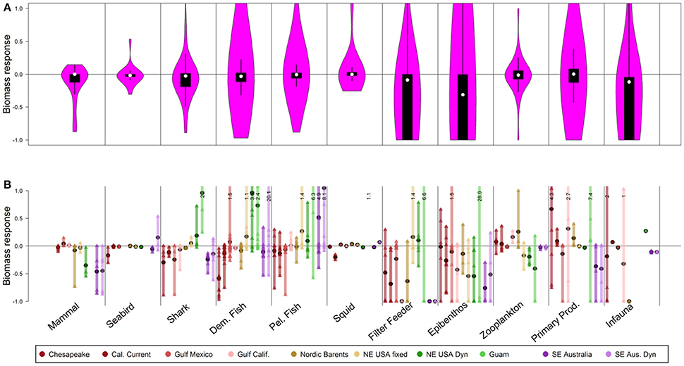
Figure 2. Biomass response of 50-year scenarios of ocean acidification, via an additional 1% mortality rate (day⁻¹) added for selected groups. (A) The shape of the violin plots shows the kernel density of biomass responses across all individual functional groups in all models. Superimposed box plots illustrate the median (white), 5th and 95th percentiles (lines), and first and third quartile (boxes). Functional group responses that exceed 1.0 (i.e., doubling of biomass and the limit of the y-axis) are truncated here, but noted in the lower panel. (B) Detailed results, with each ecosystem model represented by a unique color and ordered as shown in the legend. Vertical bars represent the range of functional group responses, grouped by guilds, within each ecosystem model. Small triangles are individual functional group responses, and black circles are the average responses per model. Functional group responses that exceed a y-value of 1.0 (i.e., doubling of biomass) are indicated with black text.

We illustrate effects of the scenarios as proportional changes in biomass, in two graphical presentations: (1) One violin plot (Hintze and Nelson, 1998) per scenario and guild, which incorporated results from all functional groups in all systems. Violin plots display the kernel density of biomass responses pooled across all model ecosystems, and include box plots to illustrate the median, 5th, 25th, 75th, and 95th percentiles. These plots provide a synoptic view of the effects of the scenarios, rather than detailed results per ecosystem. (2) Proportional change in biomass of individual functional groups within a guild for each ecosystem. These plots illustrate how responses differ between ecosystems.

Comparisons: Ecological Indicators

We calculated ecological indicators as a method to summarize ecosystem-level responses to the scenarios, beyond simple biomass responses of individual functional groups. Ecological indicators for marine systems have been summarized, discussed, and tested extensively by Fulton et al. (2005), Rice and Rochet (2005), Methratta and Link (2006), Shin and Shannon (2010), among others. From the existing literature we chose two sets of ecological indicators that summarize the ecosystem state, averaged over years 45–50 of each scenario: one set focused on properties of the ecological community and a second set focused on fisheries and economic properties (that is the most relevant to evaluate the socioeconomic effects on livelihoods and economic benefits). We used seven indicators of ecological community properties (Table 2): ratio of demersal to pelagic fish; proportion of predatory fish; mean trophic level (MTL) of biomass; the ratios of total, pelagic, and demersal biomass to primary production; and the ratio of demersal to pelagic biomass. We assessed 12 indicators of fisheries properties (Table 2): total catch; catch of fish, demersal, and pelagic species; proportion of populations above management targets (i.e., above BMSY); ratios of pelagic catch, demersal catch, and total catch to primary productivity; mean trophic level of catch; exploitation rate of fish only (summed catch/ summed biomass); exploitation rate of all target species (total summed catch/total summed biomass); and value of catch. The fisheries indicators are also directly relevant to measure the economic responses, either directly as the value of the catch or indirectly as the biomass of the catch (in total or split into pelagic or demersal catch). We present these indicators as radar plots (similar to Fulton et al., 2014), which score performance relative to the base-case scenario and illustrate the tradeoffs between indicators (i.e., between objectives). Within these radar plots, metrics are generally ordered by: ecological indicators (left), fishery indicators (right), pelagic (top), and demersal or benthic (bottom). This was an attempt to align or group the emergent properties (axes) in a simple way that has been applied in more detailed multivariate approaches elsewhere e.g. Ten Brink et al. (1991), Collie et al. (2003) and Coll et al. (2010). Note that we expect scores of certain indicators (axes) to be highly correlated (e.g., ratio of demersal to pelagic fish and ratio of demersal to pelagic biomass), therefore the axes are interdependent, and readers should consider the score along each axis separately rather than visually integrating the area covered by the radar plot.

TABLE 2

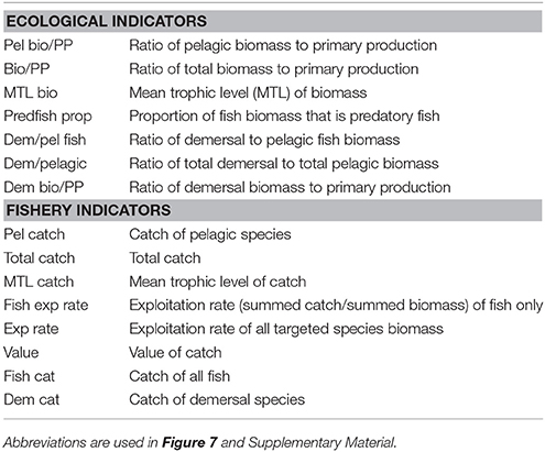
Table 2. Ecological and fishery indicators.

R-Code for Analysis

All analyses were done using the R statistical software package, and the scripts used to generate all plots are freely available on GitHub: (https://github.com/r4atlantis/common_scenarios_analysis/tree/master/sept17).

Results

Ocean acidification

Direct effects of ocean acidification on echinoderms and mollusks led to moderate median declines at the guild level (Figure 2A, white points, median declines of 31% for the epibenthos guild, 9% for the filter feeder guild, and 12% declines for infauna), but severe declines for particular “losers” throughout the food web, i.e., a quarter of functional groups in the epibenthos, filter feeder, and infauna guilds exhibited 100% declines, i.e., extirpation (Figure 2A, lower extent of boxplots). Following Kroeker et al. (2013), we also specified direct effects on calcifying algae, corals, and coccolithophores in models that included those groups (i.e., Guam and Gulf of Mexico). The Guam model, which is entirely focused on shallow (0–30 m) coral reef ecosystems, had calcifying crustose coralline algae decline to 13% of the base value, while the branching and massive coral groups both declined to functional extinction. In our simulations, strong effects of acidification were included beginning in year 1 of the simulation, and in most cases (e.g., filter feeders, Figure S31) this resulted in strong direct impacts within the first 1–3 years, followed by stable biomasses at the guild level.

Indirect food web effects of acidification similarly emphasize slight declines at the guild level (≤3% declines for mammals, seabirds, sharks, demersal, and pelagic fish guilds, Figure 2A, white points), but large declines for the lower quartile of functional groups (Figure 2A, lower extent of boxplots). These “losers” under ocean acidification declined 3–19% (lower quartile of mammals, seabirds, sharks, and demersal and pelagic fish guilds), with strongest impacts on mammals, shark, and demersal fish guilds (declines of 12, 19, and 11%, respectively, at the lower quartile). Individual mammal, shark and demersal fish functional groups declined by more than 50%. “Winners” under ocean acidification were relatively rare, particularly for vertebrates, with the upper quartile of mammals, sharks, seabirds, demersal fish, and pelagic fish guilds gaining <3%. The dynamic responses to these food web effects were somewhat gradual, typically reaching stable values (in most cases) by approximately year 10–30 (e.g., demersal fish, Figure S32).

The results identify individual ecosystems (Figure 2B) that may be more vulnerable and responsive to ocean acidification than other regions. The Chesapeake Bay and California Current appeared particularly vulnerable, exhibiting stronger declines in seabirds, sharks, demersal fish, and pelagic fish under ocean acidification (Figure 2B, averages represented as black circles) than other ecosystems. On the other hand, the Northeast USA and Southeast Australia may be less vulnerable to acidification: increases in demersal fish were predicted by the models for the Northeast USA and by the Southeast Australia model with dynamic fishing effort.

Though mammal, shark, and demersal fish had the largest responses at the guild level (Figure 2A), within individual models (Figure 2B) there was high variability among functional groups, with coefficients of variation as high as 2.9 for the mammal guild, 2.4 for shark, and 5.3 for the demersal-fish guild. Higher variability in response at the functional group or species level (Figure 2B) compared to more moderate responses at the guild level (Figure 2A) suggests compensatory responses (“winners” and “losers”) and functional redundancy within the guilds. Differences in functional group behavior within a guild primarily reflect differences in diets. As an example, groups within the Gulf of Mexico and Southeast Australia Bay demersal-fish guilds showed both strong positive and strong negative effects because demersal-fish diets vary widely, with some fish being dependent on calcifiers, while others have no such dependence.

Results from the less severe ocean acidification scenario with 0.5% day⁻¹ mortality rates for sensitive species were consistent with patterns displayed in the 1% ocean acidification scenario, but the responses were lower in magnitude (Figure S1).

Spatial Management

Similar to the OA scenario, for the MPA scenario the guild-level median responses were on average quite modest (<1%), but effects on individual groups occurred throughout the food web (Figure 3A). Some sharks, demersal fish, and pelagic fish benefited from MPAs, and though the median response was minimal, “winners” within these guilds increased 5, 13, and 11% respectively (3rd quartile) with rare increases up to 21, 34, and 46% (95th percentile for each of these guilds respectively). An increase in predation by seabirds and some fish led to declines in the most responsive zooplankton groups, but these were rare (i.e., 15% decline for 5th percentile). Invertebrates were not especially likely to benefit from the MPAs, though the relative insensitivity of the epibenthos and filter feeder guilds is likely due to our aggregation of harvested and unharvested stocks within the same guilds. The dynamic responses to MPAs were somewhat gradual, reaching stable values of guild-level biomass (in most cases) by approximately year 10–30 (e.g., sharks, Figure S33).

FIGURE 3

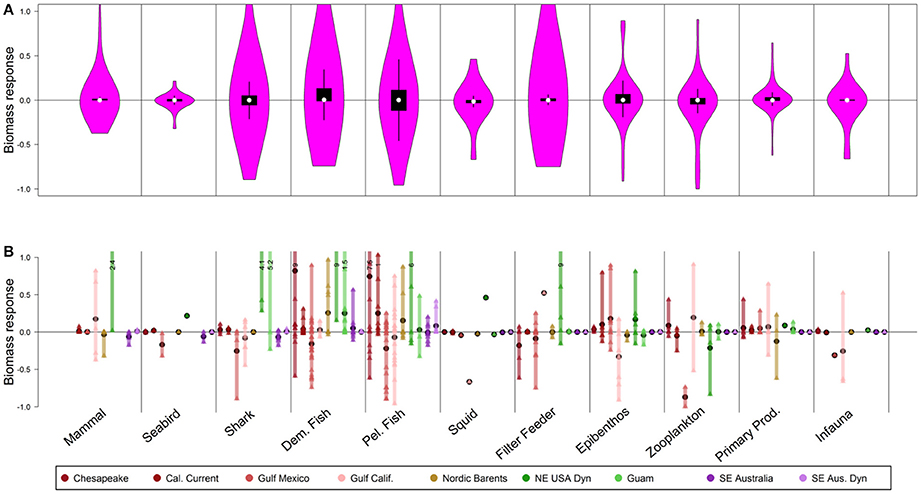
Figure 3. As in Figure 2, but representing biomass response of 50-year scenarios of spatial management closing 50% of continental shelf (<250 m depth) to fishing. Note that the proportion of the model domain closed varies depending upon depth of the system (see Table S1).

Unlike the ocean acidification scenario, responses to MPAs tended to be symmetrical within guilds, meaning that declines in “losing” species (lower quartile of responses) were matched by increases in winners (upper quartile of responses, Figure 3A). For instance, across guilds of mammal, seabirds, shark, demersal fish, and pelagic fish, the upper quartiles of responses ranged from 1 to 11% and the lower quartile exhibited almost symmetrical declines of 0–11%. Partially this reflects guilds that comprise a mix of harvested stocks (which typically benefited from MPAs) and unharvested stocks (which were more likely to decline under MPAs). Demersal fish exhibited this pattern; though they might be expected to respond strongly to MPAs (van Denderen et al., 2016), they displayed a mix of both positive and negative responses (Figure 3A). The pelagic fish and shark guilds also highlight this symmetrical response (11% increases for “winners” in the pelagic fish guild and 11% declines for “losers”; 5% increases for “winners” in the shark guild and 5% declines for “losers”), due to mix of harvested/unharvested species and compensation within the guild that is evident at the functional group or species level (Figure 3B).

Differences in responses across ecosystems can be understood in the context of the characteristics of those individual ecosystems and constituent functional groups (i.e., groups of species with similar life history, diets, and predators). For instance, the 50% MPAs led to strong increases (>20%) in certain mammal and shark functional groups, but only in a few systems (Figure 3B). Ecosystems that responded most dramatically to this scenario (i.e., those with at least one functional group responding by at least 100%) are shallow systems where encapsulating 50% of the shallow region in an MPA closed large fractions of the total model domain. For example, the shallow Chesapeake Bay, Guam, and NE USA regions exhibited strong increases in demersal fish or shark. In contrast, the response in SE Australia was much lower as the shelf makes up a minority of the total model area, and there is already extensive fisheries zoning in place, so the MPA scenario represented a smaller incremental change than in other models.

Patterns for seabirds, mammals, zooplankton, epibenthos, and filter feeders in the 50% MPA scenario were consistent with patterns from the scenarios closing 10 and 25% of the continental shelf to fishing (Figures S2, S3), with lesser magnitude of responses when scenarios involved these smaller closed areas.

Fishing Mortality

Doubling fishing on small pelagic fish (forage fish that some argue should be fished at lower levels to ensure food for larger predators like birds, marine mammals, and larger fish, Figure 4A) had minimal direct impacts at the guild level; negative effects were primarily limited to a few predator groups (Figure 4B) rather than extending throughout the food web. Median responses across all functional groups were ≤2%, including for the pelagic-fish guild (which aggregates both small and large pelagic fish). “Losers” within the pelagic-fish guild (lower quartile) declined by 6%, and declines in this lower quartile for mammals, birds, sharks and demersal fish were also only 1–4%. The models predicted some instances of compensatory increases in non-harvested pelagic fish, but these were rare (even 95th percentile has only 10% gain).

FIGURE 4

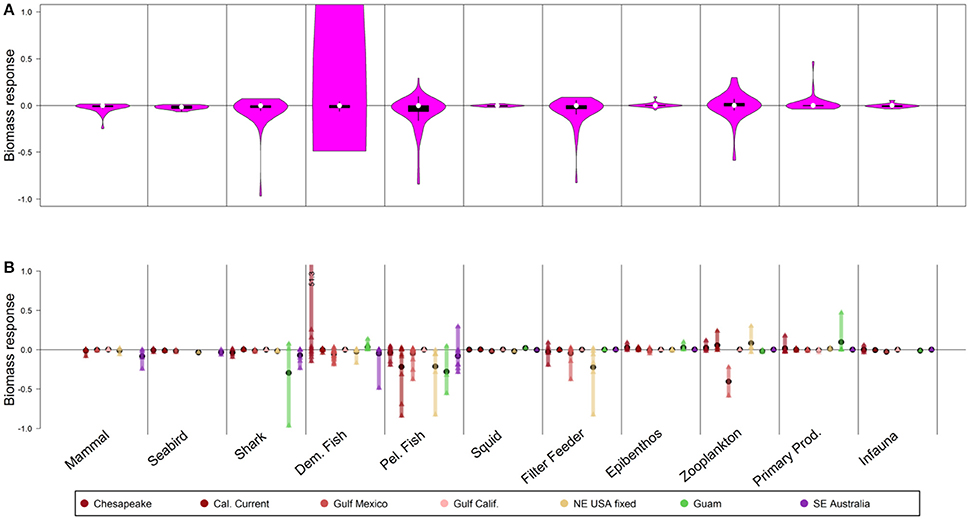
Figure 4. Biomass response to 50-year scenarios with 2× fishing mortality on small pelagic fish. Panel explanations as in Figure 2.

Guild-level responses to this scenario (Figure S34) and other fishing mortality scenarios (Figures S35–S37) demonstrate stable values of guild-level biomass (in most cases) by approximately year 10–30. This was true for species directly manipulated with fishing mortality, and for those responding to indirect, trophic effects.

At the level of individual ecosystems (Figure 4B), sharks declined strongly in Guam due to increased fishing on small pelagic fish, but this was not evident in the other, deeper systems. In the NE USA, the demersal fish guild declined as small pelagic fish were depleted (Figure 4B), and results from the Gulf of Mexico also suggested declines for some demersal fish groups; nonetheless, the aggregate prediction from the models was minimal responses by demersal fish (interquartile range from [−0.02 to 0], Figure 4A). In SE Australia, the more intensive fishing of small pelagics led some of their predators to shift consumption to mesopelagic fish, which in turn had negative impacts on some demersal fish that also consume mesopelagics (though this impact was small). In contrast to this, in Chesapeake Bay (Figure 4B) increased fishing on small pelagic fish shifted energy to the benthic food web and demersal fish, including Atlantic croaker (Micropogonias undulatus). Still, increasing fishing mortality on small pelagic fish generally affected fewer functional groups (directly and indirectly) than decreasing fishing mortality (Figures S4, S5).

Results were fairly insensitive to the manipulation of fishing on invertebrates only, and doubling fishing on invertebrates led to minimal responses at the guild level (<2% median response for any guild, including invertebrate guilds, Figure 5A). “Losers” (lower quartile of responses) included epibenthos (such as harvested crabs) that declined 10%, with rare instances of stronger declines (26% declines for the 5th percentile of epibenthic functional groups, Figures 5A,B). Note that the invertebrate functional groups here often aggregate harvested and unharvested species, thus total increases in fishing mortality at the guild level were often small. Within individual models (Figure 5B), strongest declines due to the direct effect of increased invertebrate fishing were for epibenthos in the California Current and Gulf of Mexico (where these include harvested crabs and shrimp).

FIGURE 5

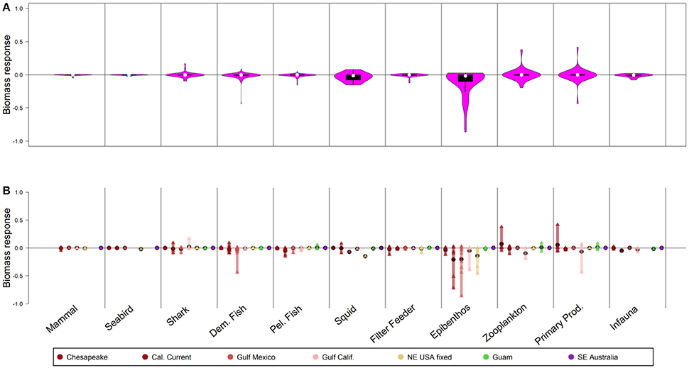
Figure 5. Biomass response to 50-year scenarios with 2× fishing mortality on invertebrates. Panel explanations as in Figure 2.

Removing fishing from invertebrates led to, at most, 3% median increases for invertebrates (epibenthos guild) and 1% increase in biomass of other guilds (Figure S6). The effects of halving fishing on invertebrates were intermediate between the base case and the scenario with removal of all fishing (Figure S7). Removing fishing on invertebrate groups caused stronger responses than doubling fishing; this pattern was also observed in manipulations of fishing on small pelagic fish.

Halving fishing mortality on demersal fish and sharks (Figure 6A) led to direct impacts on functional groups that are targeted by these fisheries, but minimal effects at the guild level and few indirect effects. The models predicted a median increase of 1% for the shark guild and 4% for the demersal fish guild, but “winners” (upper quartile, typically fishery target species) increased 20% (demersal fish) and 3% (sharks). In some instances, shark and demersal fish functional groups declined under this scenario (Figure 6A), but this was rare (interquartile range from [0–3%] to [0–20%], respectively) and occurred in cases with little fishing mortality on these particular groups in the base case. Overall, as for the other scenarios, halving fishing mortality on demersal fish and sharks led to moderate responses at the guild level (Figure 6A), and stronger responses for individual functional groups or species (Figure 6B).

FIGURE 6

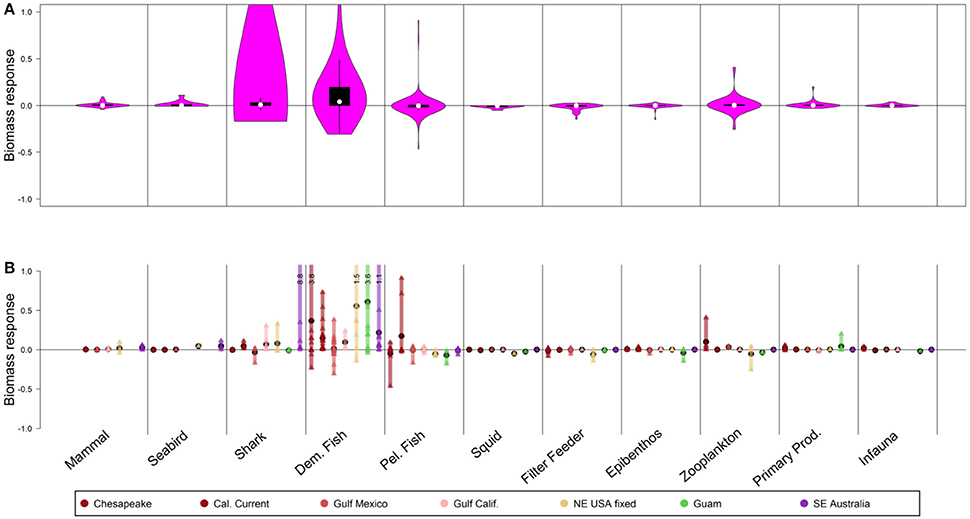
Figure 6. Biomass response to 50-year scenarios with 0.5× fishing mortality on demersal fish. Panel explanations as in Figure 2.

Increases in demersal fish groups were strongest in three shallow or continental shelf systems: NE USA, Guam, and Chesapeake Bay (Figure 6B). Indirect effects of decreased fishing on demersal fishes were minimal on lower trophic levels that are found in demersal fish diets such as zooplankton and epibenthos.

Similar to the scenarios altering fishing for small pelagic fish or invertebrates, effects of reducing demersal fish harvest led to stronger responses than did increasing demersal fish harvest. For instance, completely removing fishing on these groups (Figure S8) led to stronger median responses (2% increase in sharks and 14% increase in demersal fish) and stronger responses of particular functional groups (i.e., 95th percentile exhibiting increases of 5, 6, 46, and 117% for mammals, seabirds, sharks, and demersal fish, respectively). Also, in Figures S9–S15 the additional results of the following six scenarios runs are shown: doubling fishing mortality on demersal fish (Figure S9), no fishing mortality for large pelagic fish (Figure S10), 0.5 × fishing mortality for large pelagic fish (Figure S11), doubling fishing mortality for large pelagic fish (Figure S12), no fishing mortality for all groups (Figure S13), 0.5 × fishing mortality for all groups (Figure S14), and doubling fishing mortality for all groups (Figure S15).

Ecological and Fishery Indicators—Emergent System Properties

Ecological and fishery indicators (Methratta and Link, 2006; Fay et al., 2013) were calculated to illuminate the indirect, trophic effects, socioeconomic effects, and emergent system responses to the scenarios (Table 2). These indicators retain the ecosystem-specific details (lower panels in Figures 2–6), rather than aggregating across ecosystems (as in upper panels of Figures 2–6); thus predictions for these indicators capture the wide diversity of responses across ecosystems and identify the ecosystems most vulnerable or prone to tradeoffs.

Ocean acidification and MPA scenarios caused more substantial ecological and fishery tradeoffs than scaling fishing mortalities on some or all guilds (Figure 7 and Figures S16–S18), consistent with the more substantial biomass impacts predicted by the ocean acidification and MPA scenarios (Figures 2–6). Excluding Guam and SE Australia (discussed below), predicted impacts of ocean acidification on ecological and fishery metrics ranged from −86% to +152% (Figure 7A). Strongest negative ecological impacts of ocean acidification were evident for the Chesapeake Bay and the Norwegian and Barents Sea, primarily on the benthic community. The Chesapeake Bay also exhibited a strong decline in catch and value, as did the NE USA under the constant fishing scenario.

FIGURE 7

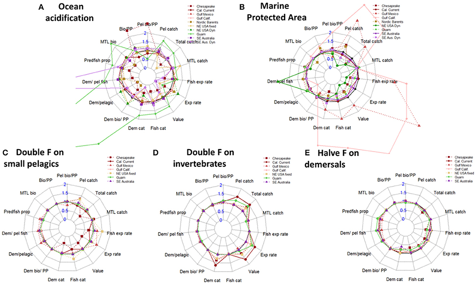
Figure 7. Ecological and fishery indicators for scenarios. Metrics are generally ordered by: Ecological indicators (left), fishery indicators (right), pelagic (top), and demersal (bottom). (A) Ocean acidification, via an additional 1% (day⁻¹) mortality rate added for selected groups. Truncated values: Guam Dem/pelagic = 8.4; SE Aus. Dyn Dem/pel fish = 6.4. (B) Spatial management closing 50% of continental shelf (<250 m depth) to fishing. (C) Doubling fishing on small pelagic fish. (D) Doubling fishing on invertebrates. (E) Halving fishing rates for demersal fish.

Guam and SE Australia responded strongly to ocean acidification, but for some ecological and fishery metrics these responses were contrary to those for other ecosystems (Figure 7A). Under ocean acidification, Guam exhibited increases in ecological metrics related to the demersal community, and subsequent increases in Catch of demersal species and Value of catch. In SE Australia, the Ratio of demersal to pelagic fish increased, but the Ratio of demersal to total pelagic biomass (all species including invertebrates) declined. Catch of demersal species therefore declined strongly in the SE Australia dynamic effort model as fishing fleets shifted to pelagic and benthopelagic stocks (in the model with constant fishing rates, fleets change their species mix but remain focused on demersals).

MPAs generally led to moderate increases in ecological metrics related to demersal species, but stronger declines in economic metrics (Figure 7B). Shallow shelf systems were strongly impacted by the MPA scenarios. For instance, under the 50% MPA the NE USA model exhibited a large increase in demersal-fish biomass and declines in metrics of catch, value, and exploitation rate. Similar declines in catch and fishery value were evident for Chesapeake Bay (our shallowest system, with a full 50% of model domain closed under this scenario). The Gulf of California and Gulf of Mexico both exhibited large increases in pelagic and demersal catches, fishery value, and exploitation rates under the 50% MPA (Figure 7). This was due to stock recovery in this scenario for these two systems. Additionally, in the Gulf of Mexico menhaden (Brevoortia patronus, an abundant forage fish) experienced an increase in biomass.

Ecological indicators generally responded modestly to the fishing mortality scenarios, with stronger economic responses for metrics (e.g., value of catch, total catch, pelagic catch, demersal catch) directly reflecting impacts on fished species and the importance of invertebrate fisheries in each ecosystem (Figures 7C–E and Figures S19–S30). For instance, doubling fishing on small pelagic fish led to a smaller than 10% change in most ecological indicators, with at most ~22% declines in the Ratio of pelagic biomass to primary production in the Gulf of Mexico (Figure 7C). Increased fishing on small pelagic fish generally led to increases in fishery metrics related to pelagic catch and total value, except for the Chesapeake Bay and California Current. Similarly, doubling fishing on invertebrates (Figure 7D) led to little change in ecological metrics, but led to increases in Catch of pelagic species (e.g., for squid in the California current), as well as for Catch of demersal species (crabs and lobsters in NE USA and Chesapeake Bay) and Value of catch (for instance driven by scallops and lobster in the NE USA and Dungeness crab in the California Current). Halving fishing for demersal species (Figure 7E) caused slight increases for most systems in Ratios of demersal to pelagic biomass or Ratios of demersal biomass to primary production. One exception was for the Gulf of Mexico, where these ratios declined slightly (this was due primarily to declines in a single demersal fish group (Deep Serranidae); most other demersal fish in this model scenario increased in abundance or were stable). Halving fishing for demersal species caused less than a 5% decline in most fishery metrics (other than the direct metric of demersal fishery catch), but with slightly stronger declines in fishery metrics for Guam (where total harvests and value are dominated by nearshore, demersal species).

Discussion

Here, we build on previous efforts to compare marine ecosystems (Megrey et al., 2009c; Link et al., 2012) by applying a global set of ecosystem models that can predict the tradeoffs inherent to three opportunities and challenges for EBM: ocean acidification, MPAs, and altering the mix of fishing effort across species. The most striking result is that across these eight ecosystems the Atlantis ecosystem model projections suggest stronger impacts from ocean acidification and MPAs than from altering the mix of fishing effort, both in terms of guild-level biomass and in terms of indicators of ecological and fishery structure. Even then, the vast majority of the impacts are moderate at the species or group level and dampened further at more aggregated taxonomic levels (guilds). This demonstrates the stability of considering higher levels of hierarchy (Fogarty et al., 2012; Link et al., 2012). The opportunity to manage at the guild level, taking advantage of greater stability there, merits further consideration. Biotic guilds are intriguing (Ross, 1986), as they show within guild compensation by component taxa in response to a dynamic environment (Auster and Link, 2009). There is clearly greater stability in terms of biomass, and hence catch, at an aggregate level (Duplisea and Blanchard, 2005; Fogarty et al., 2012; Link et al., 2012). This “portfolio” effect (Schindler et al., 2015), when managed for, results in less variability in catches, greater economic value, and more regulatory, economic and biotic stability. Results here show similar patterns associated with aggregate stability. These results provide fresh and useful input to regional tradeoff analysis aimed at continuing fisheries exploitation under increased ocean acidification. Proposing harvest policies, testing them, and managing at this aggregate or guild level (while still complying with single species mandates) through managing species complexes (Gaichas et al., 2017) or setting ecosystem biomass caps (Link, 2018) undoubtedly merits further exploration in inter-sectoral tradeoff analyses and is clearly supported as something that has observable benefits from our results.

Ocean acidification effects simulated in the eight global regions here led to indirect trophic effects, which often radiated to additional species including predators; the effects were typically negative rather than positive, but occurred at the level of particular species (or functional groups). At the aggregated level of guilds, compensatory effects led to average responses that were minimal. Our results are consistent with previous modeling (Kaplan et al., 2010; Griffith et al., 2011; Marshall et al., 2017) that suggests that if ocean acidification leads to direct mortality on benthic invertebrates, indirect impacts will evolve on predatory fish and dependent demersal fisheries. Divergence from this trend was apparent, however, most notably for the NE USA, where Fay et al. (2017) predict strong impacts of ocean acidification on benthic fish. Simulations for the NE USA here run counter to this, but illustrate a key uncertainty in our understanding of direct ocean acidification effects. In Fay et al. (2017), deposit feeders (e.g., amphipods, isopods) are assumed to be directly affected by ocean acidification, while in our scenarios they are not, and in fact increase by approximately 10–15%, leading to an increase in forage available for predators such as demersal fish. This illustrates the need for improved, direct process studies of ocean acidification effects on all life stages of abundant forage species such as these deposit feeders, and also euphausiids (see McLaskey et al., 2016), as well as consistent application of such studies across ecosystem models.

Ecological tradeoffs inherent in MPAs (Fulton et al., 2015) evolved across our eight modeled ecosystems, but at the level of individual species or groups (identifying “winning” species that benefit and “losing” species that decline), rather than at the more aggregated guild level. This is similar to the effects of ocean acidification, except that more “winners” were apparent in our MPA scenarios than OA scenarios. Additionally, because we simulated MPAs as closures to fishing of the continental shelf (e.g., 50% closure of area <250 m depth), shallow systems were more strongly impacted by these scenarios, as were systems for which the “base case” or status quo largely lacked spatial fishery management. Overall, MPAs led to declines in most indicators of fishery yield and value, highlighting that in addition to trade-offs across species, there are trade-offs among ecological and economic considerations (Kaplan et al., 2012). Exceptions to this were for two systems (Gulf of Mexico and Gulf of California) that have high exploitation rates under base case conditions. In these systems, the relaxation of fishing pressure led to recovery of particular species (but not necessarily entire ecological guilds) that led to long-term increases in catch and harvest value.

Our scenarios that altered fishing effort across species caused less drastic responses than did ocean acidification or MPAs; this was true in terms of biomass and also indicators of fishing and ecological response. The responses of birds, mammals, or sharks to these fishing scenarios were inconsistent across systems, and the average responses (at the guild level) were minimal. Furthermore, the exact mechanisms of change were highly system dependent (e.g., SE Australia, Chesapeake Bay). Doubling or halving of existing fishing rates on all harvested forage stocks (allowing other forage species to compensate in some cases) did not lead to strong impacts on predators in most cases. Other global ecosystem modeling efforts (Smith et al., 2011; Pikitch et al., 2014) as well as field observations (Cury et al., 2011; Bertrand et al., 2012; McClatchie et al., 2016) suggest that certain seabirds and marine mammals may be more vulnerable to the availability of forage stocks, particularly when we consider appropriate spatial scales of interaction (Sydeman et al., 2017). In contrast to this, a synthesis of USA fish, marine mammal, and bird populations has recently argued against this vulnerability for most predators (Hilborn et al., 2017). Within the context of this debate, our results suggest minimal guild-level impacts of forage depletion, under three assumptions within the simulations: (1) fishing focuses only on a subset of (currently targeted) forage species and at most 2 × baseline rates; (2) fisheries were not concentrated near seabird and mammal breeding sites; and (3) models such as Atlantis include realistic age structure and density dependence (Walters et al., 2016). However, the sensitivity of individual species (or functional groups) in our models argues for future modeling at the species level (e.g., Punt et al., 2016), perhaps including spatial overlap and movement of mammals or birds and forage (Boyd et al., 2014).

Increased fishing for invertebrates (including squid, shrimp, crabs, and shellfish) consistently led to higher catch and value in most of our simulated ecosystems, with minimal effects on indicators of ecosystem structure. In contrast to this, Eddy et al. (2017) found that increasing fishery exploitation rates of invertebrates using a global suite of Ecopath with Ecosim (EwE) models had considerable ecosystem wide effects, though typically those increases in fishing rates and declines in invertebrate biomass were stronger than what we tested here. Our results for fishing scenarios (particularly in Supporting Information) demonstrated that removal of fishing caused larger changes to the ecosystem and fishery structure than did doubling of fishing. We hypothesize this is because many of these systems have long histories of fishing with even higher fishing pressure than today and are currently quite far from their original unfished states. Strong shifts in the ecosystem may occur at relatively low fishing rates (Samhouri et al., 2010). Overall, our results from the fishing scenarios suggest the necessity of cross-sectoral EBM: decisions regarding fishing rates, effort, and catches can be overwhelmed by larger multi-sector changes related to spatial management, and by the threat of global change.

Comparing the ecological and catch indicators gives insights into tradeoffs between socioeconomic effects of fishing (on the fishing industry and fishing communities) and ecological changes as seen in the response to various changes in fishing pressure. The indicators used were chosen based on studies that have analyzed their merits and usefulness (Fulton et al., 2005; Rice and Rochet, 2005; Methratta and Link, 2006; Shin and Shannon, 2010), and although several are interdependent (e.g., “demersal catch” and “fish catch” are subsets of “total catch”), they are included as they allow splitting the responses into meaningful ecological or fisheries sub-units. This can be seen from Figure 7A where the strong decline in total catch for the NE USA Fixed and Chesapeake Bay was driven by the strong decline in demersal catches while the pelagic catches remained closer to the base case. Similar interdependencies are present between the “Bio/PP,” “Pel Bio/PP,” and “Dem bio/PP,” between “Exp rate” and “Fish exp rate,” and between the “MTL bio” and “MTL catch” indicators. Though these interdependencies can be easily interpreted, we caution against visually “integrating” the area of the radar plots, and point readers to multivariate methodologies that distil such indicator scores into independent axes, e.g. Ten Brink et al. (1991); Collie et al. (2003), and Coll et al. (2010). The strength and presence of tradeoffs among indicators when analyzed visually using radar plots may also be influenced by the ordering of indicators around the axes of the plot (e.g., Shin et al., 2010). Ideally the set of indicators chosen to be presented in tradeoff plots should reflect the full set of management objectives; most sensibly this selection and summary of indicators is probably achieved in partnership with managers and stakeholders (Punt, 2015). In part the lack of balance across our indicators reflects differing levels of complexity in human components of the range of modeled ecosystems, and the need to compute a common set of measures across ecosystems. Specific analysis of the radar plots showed that doubling fishing mortality on invertebrates gave the most consistently positive results across models (Figure 7D), with no decreases in any of the catch indicators and with indicator values >150% in several models for Pelagic catch, Total catch, Exploitation rate, Value, and Demersal catch. None of the ecological indicators showed a strong response (all were close to 100%, e.g., equal to the base case) for any of the models. A similar, but less clear pattern could be seen for the scenario doubling fishing mortality on small pelagics, but here the positive responses were not so apparent, and one model, the Chesapeake Bay responded negatively for several of the catch indicators. Again, all models had no responses (close to 100%, e.g., they were equal to the base case) for the ecological indicators. Lastly, halving the fishing mortality on demersals gave little response on either ecological or catch indicators. These results indicate that the marine ecosystems modeled in this study are more resilient and less affected by changes in fishing pressure than are the fishing industry and fishing communities, and that the most positive effects may be achieved by increasing fishing pressure on invertebrates. However, it is worth inserting a note of caution here. Invertebrates are typically represented as bulk biomass pools in Atlantis (and other ecosystem-level models) and as such may not be capturing their ecological processes with sufficient nuance. Consequently, these findings should be taken as preliminary indicators only and more detailed case-specific consideration should be given to any particular system looking to significantly increase pressure on invertebrate stocks, so as to avoid unintended negative consequences (Eddy et al., 2017).

Our results give an indication of potential tradeoffs that need to be further evaluated and studied for each ecosystem separately before being proposed as management action, but clearly illustrate how ecosystem modeling can be used to highlight the most interesting management action among a suite of possible alternatives. Specifically, our results indicate that any fisheries management or area-based protection measures to be considered first have to take into consideration the effects of OA, as the effects of OA greatly overwhelm effects of managing human activities. Since OA has its greatest effect on the epibenthos guild, it can be hypothesized that the combined effect of OA and any increase in fisheries targeting epibenthic organism (e.g., molluscs or crustaceans) would lead to aggregated impact on the epibenthic guild. Thus, management actions that are taken without considering the effects of OA may have unforeseen or even detrimental effects. By running combination scenarios OA with fisheries management and marine protection more definite advice on the potential trade-offs can be elucidated.

There is value in a comparative approach (Megrey et al., 2009b; Murawski et al., 2010) and in using common indicators (Shin et al., 2010). Marine ecosystems are complex, and understanding their fundamental processes, functioning, dynamics, and structures is often challenging. Monitoring and experimentation are essential, but logistically difficult at appropriate scales and extremely limited for many regions. Comparison of modeled ecosystems facilitates learning and understanding about marine ecosystems in that common scenarios, tested across a range of ecosystem types, can confirm or elicit common responses and highlight distinctions. A common indicator set facilitates comparison, helps researchers elucidate understanding of marine ecosystems, and highlights common problem areas in terms of modeling skill, understanding, or major pressures. Common scenarios also provide the community of practitioners a set of standards to consistently interpret status of ecosystems, results of forecasts, and relative importance of responses to common scenarios and pressures. The debate over indicator selection (Rice and Rochet, 2005; Shin et al., 2010) seems to be settling in this community of practice, with a suite of indicators similar to those presented here typically emerging. The next challenge is to convert a common set of indicators into thresholds or control rules (Link, 2005; Samhouri et al., 2010; Large et al., 2015; Tam et al., 2017) that can be tested across ecosystems to inform decision-makers when action is needed and what level of action would be appropriate.

Caveats and Next Steps

While common patterns are evident across many of the modeled systems, it is appropriate to say that this may be because a single modeling framework was used. While the models were of different ecosystem types and of radically different spatial extents, they were all implemented within a single framework, Atlantis. Interpretation of the results requires caution and preferably with broader validation or verification of the general patterns of outcomes. While cross-ecosystem comparisons (Murawski et al., 2010) (within a common modeling approach) can provide some insight into responses to future scenarios for management and ocean change, a complementary approach is to apply multi-model comparison (Gårdmark et al., 2013; Townsend et al., 2014; Ianelli et al., 2016). Considering multiple model frameworks with distinct underlying structural assumptions can quantify how decisions about taxonomic aggregation and ecological and fishery parameterization influence the strength of model response to perturbations (Pinnegar et al., 2005; Walters et al., 2016). Finding common patterns in the results of such ensembles gives more confidence in the general robustness of those findings and thus overcomes uncertainties due to model choice.

The current results examine the effects of each of the three drivers separately. In reality these interact and the present analysis should be expanded to run scenarios combining increasing OA with marine protection and changes in fisheries. However, the number of scenarios to run would increase dramatically and were unfortunately outside the scope and capacity of the present experiment.

In interpreting these results, it is important to acknowledge the specific limitations of the fishing and fishery management scenarios implemented (Fulton et al., 2011), the lack of downscaled oceanographic projections informed by global earth system models (e.g., Marshall et al., 2017) in most regions, and the need for consideration of interactions between ocean acidification, ocean warming, range shifts, and other aspects of global change (Griffith et al., 2012; Fernandes et al., 2017; Ihde and Townsend, 2017). While more dynamic representations of ocean acidification are possible using Atlantis (Marshall et al., 2017), this degree of complication was beyond available resources for some model locations. Similarly, the implementation of fishing fleet effort dynamics required to explore some of the more nuanced responses to spatial management requires a level of resources and information not available for all the model locations. Consequently, our scenarios for MPAs were simple, closing large areas to fishing but without displacement of fishing effort (Agardy et al., 2011); more detailed modeling of spatial fleet dynamics has been undertaken in only some Atlantis applications (e.g., NE USA, SE Australia, also Girardin et al., 2017). More realistic MPA scenario modeling is needed to evaluate the effects of population spill overs from closures, fishing effort reallocation, as well as to elucidate the trade-offs between biodiversity protection and loss of economically valuable fishing grounds. Our fishing scenarios are also crude adjustments of fishing mortalities for small pelagic fish, invertebrates, and demersal fish; fully envisioning future scenarios for fisheries has been considered at a global scale (Delgado et al., 2003; Merino et al., 2012) but should be translated to each region given the local fishery and economic context.

Sensitivity testing of key parameters determining the performance of the scenarios would have added better understanding of how dependent scenario results are on parameter settings. However, due to the long run times of the models, such sensitivity analyses were not feasible to carry out.

Our global analysis identifies some potential options and issues that need more in-depth and careful exploration using regional models and more specific methods. Full EBM trade-off analysis should also encompass all human uses of marine ecosystem to address multi-stakeholder perspectives. Moreover, the current Atlantis models take no account for cross border management issues (many are only located in a single EEZ) which in practical real-world management are one of the most difficult issues to resolve in achieving holistically sustainable EBM.

Conclusion

Our applications of the Atlantis end-to-end ecosystem model evaluate how different trends in the future ocean conditions may lead to key tradeoffs among species, management actions, and societal choices. Evaluating tradeoffs is a pillar of EBM, and our results here underscore a point from Link (2010): fisheries management can negotiate allocation of harvest among stocks and sectors but must exist within the reality of “non-negotiable” limits set by ecosystem productivity. Our results suggest that even if overall, aggregated levels of productivity and biomass are relatively stable in the near future, as simulated here, scenarios for ocean acidification can sharply decrease the productive capacity of individual species and functional groups, thus limiting the potential tradeoff options for fisheries and marine conservation. While acknowledging that the use of zoning for fisheries and conservation may lead to some benefits (Fulton et al., 2014), it must also be acknowledged that (as shown here) closing areas for fishing as part of implementing marine protection has negative impacts on fisheries and the socioeconomics of the fishing sector. Marine protected areas (whether driven by fishery management or multi-sector considerations such as energy extraction and species conservation) similarly shift the spatial pattern of productivity by altering fishing mortality on particular groups. Altering fishing effort has greater effect on the socioeconomics of the fishing sector than on the ecosystem, indicating a resilience in the ecosystems modeled here to changes in fisheries management (which could in part be because these systems are already amongst some of the best managed globally so they are starting from a good position). The challenge of the future will be to carry out inter-sectoral tradeoff analyses that devise, test, and implement EBM strategies that detect and cope with these productivity shifts in the future and help to maintain this ecosystem resilience. A possible future scenario would be to explore whether a combination of increased OA and marine protection could have synergistic effects on the fisheries in terms of reduced catches and value of catch, or if indirect pathways would alleviate the socioeconomic effects. End-to-end models such as Atlantis can serve as strategic tools to identify vulnerable species and fisheries within particular ecosystems and serve as an important foundation for EBM tradeoff analyses. Our analysis using a suite of models spanning the Pacific and Atlantic, both hemispheres and ranging from the Arctic to the tropics has shown that these can serve as testbeds to illuminate adaptive management strategies (Fulton, 2010; Punt et al., 2014) that address multi-sector trade-offs that are robust to the coming climate-driven shifts in marine ecosystems.

Author Contributions

Conceived and designed the experiments: EO, JL, IK, SG, GF. Performed the experiments: IK, HM-L, EO, EF, MW, TI, CA, CE, RoG, GF, MS-R. Analyzed the data: IK. Contributed reagents, materials, and analysis tools: EF, IK, HM-L, KJ, EO, GF, HT, MW. Interpreted Results: IK, EO, CA, JL, SG, RaG. Wrote the paper: IK, KJ, HM-L, EO, EF, SG, GF, CE, RoG, TI, MW. Designed the model software used in analysis: EF.

Conflict of Interest Statement

The authors declare that the research was conducted in the absence of any commercial or financial relationships that could be construed as a potential conflict of interest.

Acknowledgments

This publication was an outcome of the first International Atlantis Ecosystem Modeling Summit (http://atlantis.cmar.csiro.au/; http://www/en/atlantis/Atlantis-Summit.html) which took place in Honolulu, Hawaii on December 7–11, 2015 and was convened and funded by CSIRO (Australia), NOAA Fisheries (US), and IMR (Norway) and the Norwegian Research Council. EO and CE received funding from the Norwegian Research Fund project PRIME TRADEOFFS (Cofasp ID 1277). HM-L was funded through the grant “Implementing Ecosystem-Based Fisheries Management: Two Case Studies in the Northern Gulf of California” from The David and Lucile Packard Foundation to CEDO Intercultural, and a Microsoft Azure Research Award “Exploring ecosystem-level effects of fisheries, management, and climate change in marine systems” provided cloud computing resources. KJ was funded in part by a grant from Washington Sea Grant, University of Washington, pursuant to National Oceanic and Atmospheric Administration Award No. NA15OAR4170181. GF was funded in part by a grant from the Cooperative Institute for the North Atlantic Region, Woods Hole Oceanographic Institution, pursuant to National Oceanic and Atmospheric Administration Award No. NA14OAR4320158. IK and California Current model development benefited greatly from a grant from the NOAA Ocean Acidification Program and National Centers for Coastal Ocean Science. MW and the Guam model development was funded by the NOAA Coral Reef Conservation Program. The views expressed herein are those of the author(s) and do not necessarily reflect the views of NOAA or any of its sub-agencies. We thank Dr. Kristin Marshall for comments on a draft of this manuscript.

Supplementary Material

The Supplementary Material for this article can be found online at: https://www.frontiersin.org/articles/10.3389/fmars.2018.00064/full#supplementary-material

Footnotes

1. ^https://research.csiro.au/atlantis/

References

Agardy, T., di Sciara, G. N., and Christie, P. (2011). Mind the gap: addressing the shortcomings of marine protected areas through large scale marine spatial planning. Mar. Policy 35, 226–232. doi: 10.1016/j.marpol.2010.10.006

CrossRef Full Text | Google Scholar

Ainsworth, C. H., Samhouri, J. F., Busch, D. S., Cheung, W. W. L., Dunne, J., and Okey, T. A. (2011a). Potential impacts of climate change on Northeast Pacific marine foodwebs and fisheries. ICES J. Mar. Sci. 68, 1217–1229. doi: 10.1093/icesjms/fsr043

CrossRef Full Text | Google Scholar

Ainsworth, C. H., Schirripa, M. J., and Morzaria-Luna, H. (2015). An Atlantis Ecosystem Model for the Gulf of Mexico Supporting Integrated Ecosystem Assessment. Miami, FL: NOAA. NFMS. SFSC.

Google Scholar

Ainsworth, C., Kaplan, I. C., Levin, P. S., Cudney-Bueno, R., Fulton, E. A., Mangel, M., et al. (2011b). Atlantis Model Development for the Northern Gulf of California. Seattle, WA: NOAA Technical Memorandum NMFS-NWFSC-110.

Google Scholar

Auster, P. J., and Link, J. S. (2009). Compensation and recovery of feeding guilds in a northwest Atlantic shelf fish community. Mar. Ecol. Prog. Ser. 382, 163–172. doi: 10.3354/meps07962

CrossRef Full Text | Google Scholar

Barange, M., Field, J. G., Harris, R. P., Hoffmann, E. E., Perry, R. I., and Werner, F. (2010). Marine Ecosystems and Global Change. Oxford: Oxford University Press.

Belton, B., Bush, S. R., and Little, D. C. (2016). Aquaculture: are farmed fish just for the wealthy? Nature 538:171. doi: 10.1038/538171d

PubMed Abstract | CrossRef Full Text | Google Scholar

Bertrand, S., Joo, R., Arbulu Smet, C., Tremblay, Y., Barbraud, C., and Weimerskirch, H. (2012). Local depletion by a fishery can affect seabird foraging. J. Appl. Ecol. 49, 1168–1177. doi: 10.1111/j.1365-2664.2012.02190.x

CrossRef Full Text | Google Scholar

Boyd, C., Punt, A. E., Weimerskirch, H., and Bertrand, S. (2014). Movement models provide insights into variation in the foraging effort of central place foragers. Ecol. Modell. 286, 13–25. doi: 10.1016/j.ecolmodel.2014.03.015

CrossRef Full Text | Google Scholar

Browman, H. I. (2016). Applying organized scepticism to ocean acidification research. ICES J. Mar. Sci. 73, 529–536. doi: 10.1093/icesjms/fsw010

CrossRef Full Text | Google Scholar

Bundy, A., Bohaboy, E. C., Hjermann, D. Ø., Mueter, F. J., Fu, C., and Link, J. S. (2012). Common patterns, common drivers: comparative analysis of aggregate surplus production across ecosystems. Mar. Ecol. Prog. Ser. 459, 203–218. doi: 10.3354/meps09787

CrossRef Full Text | Google Scholar

Bundy, A., Chuenpagdee, R., Boldt, J. L., de Fatima Borges, M., Camara, M. L., Coll, M., et al. (2016). Strong fisheries management and governance positively impact ecosystem status. Fish Fish. 18, 412–439. doi: 10.1111/faf.12184

CrossRef Full Text | Google Scholar

Busch, D. S., and McElhany, P. (2016). Estimates of the direct effect of seawater ph on the survival rate of species groups in the California current ecosystem. PLoS ONE 11:e0160669. doi: 10.1371/journal.pone.0160669

PubMed Abstract | CrossRef Full Text | Google Scholar

Christensen, V., and Walters, C. J. (2004). Ecopath with Ecosim: methods, capabilities and limitations. Ecol. Modell. 172, 109–139. doi: 10.1016/j.ecolmodel.2003.09.003

CrossRef Full Text | Google Scholar

Cinti, A., Shaw, W., Cudney-Bueno, R., and Rojo, M. (2010). The unintended consequences of formal fisheries policies: social disparities and resource overuse in a major fishing community in the Gulf of California, Mexico. Mar. Policy 34, 328–339 doi: 10.1016/j.marpol.2009.08.002

CrossRef Full Text | Google Scholar

Coll, M., Shannon, L. J., Yemane, D., Link, J. S., Ojaveer, H., Neira, S., et al. (2010). Ranking the ecological relative status of exploited marine ecosystems. ICES J. Mar. Sci. 67, 769–786. doi: 10.1093/icesjms/fsp261

CrossRef Full Text | Google Scholar

Collie, J. S., Gislason, H., and Vinther, M. (2003). Using AMOEBAs to display multispecies, multifleet fisheries advice. ICES J. Mar. Sci. 60, 709–720 doi: 10.1016/S1054-3139(03)00042-0

CrossRef Full Text | Google Scholar

Cooley, S. R., and Doney, S. C. (2009). Anticipating ocean acidification's economic consequences for commercial fisheries. Environ. Res. Lett. 4:024007. doi: 10.1088/1748-9326/4/2/024007

CrossRef Full Text | Google Scholar

Cury, P. M., Boyd, I. L., Bonhommeau, S., Anker-Nilssen, T., Crawford, R. J. M., Furness, R. W., et al. (2011). Global seabird response to forage fish depletion–one-third for the birds. Science 334, 1703–1706. doi: 10.1126/science.1212928

PubMed Abstract | CrossRef Full Text | Google Scholar

Delgado, C. L., Wada, N., Rosegrant, M. W., Meijer, S., and Ahmed, M. (2003). Fish to 2020: Supply and Demand in Changing Global Markets. Penang: The World Fish Center.

Google Scholar

Drinkwater, K. F., Mueter, F., Friedland, K. D., Taylor, M., Hunt, G. L. Jr., Hare, J., et al. (2009). Recent climate forcing and physical oceanographic changes in northern hemisphere regions: a review and comparison of four marine ecosystems. Prog. Oceanogr. 81, 10–28. doi: 10.1016/j.pocean.2009.04.003

CrossRef Full Text | Google Scholar

Duplisea, D. E., and Blanchard, F. (2005). Relating species and community dynamics in an heavily exploited marine fish community. Ecosystems 8, 899–910. doi: 10.1007/s10021-005-0011-z

CrossRef Full Text | Google Scholar

Eddy, T. D., Lotze, H. K., Fulton, E. A., Coll, M., Ainsworth, C. H., de Araújo, J. N., et al. (2017). Ecosystem effects of invertebrate fisheries. Fish Fish. 18, 40–53. doi: 10.1111/faf.12165

CrossRef Full Text | Google Scholar

Fay, G., Large, S. I., Link, J. S., and Gamble, R. J. (2013). Testing systemic fishing responses with ecosystem indicators. Ecol. Modell. 265, 45–55. doi: 10.1016/j.ecolmodel.2013.05.016

CrossRef Full Text | Google Scholar

Fay, G., Link, J. S., and Hare, J. A. (2017). Assessing the effects of ocean acidification in the Northeast US using an end-to-end marine ecosystem model. Ecol. Modell. 347, 1–10. doi: 10.1016/j.ecolmodel.2016.12.016

CrossRef Full Text | Google Scholar

Fernandes, J. A., Papathanasopoulou, E., Hattam, C., Queirós, A. M., Cheung, W. W. W. L., Yool, A., et al. (2017). Estimating the ecological, economic and social impacts of ocean acidification and warming on UK fisheries. Fish Fish. 18, 389–411. doi: 10.1111/faf.12183

CrossRef Full Text | Google Scholar

Fogarty, M. J., Overholtz, W. J., and Link, J. S. (2012). Aggregate surplus production models for demersal fishery resources of the Gulf of Maine. Mar. Ecol. Prog. Ser. 459, 247–258. doi: 10.3354/meps09789

CrossRef Full Text | Google Scholar

Fu, C., Gaichas, S., Link, J. S., Bundy, A., Boldt, J. L., Cook, A. M., et al. (2012). Relative importance of fisheries, trophodynamic and environmental drivers in a series of marine ecosystems. Mar. Ecol. Prog. Ser. 459, 169–184. doi: 10.3354/meps09805

CrossRef Full Text | Google Scholar

Fulton, E. A. (2001). The Effects Of Model Structure And Complexity On The Behaviour And Performance Of Marine Ecosystem Models. Ph.D Thesis, School of Zoology, University of Tasmania, Hobart, TAS.

Google Scholar

Fulton, E. A. (2010). Approaches to end-to-end ecosystem models. J. Mar. Syst. 81, 171–183. doi: 10.1016/j.jmarsys.2009.12.012

CrossRef Full Text | Google Scholar

Fulton, E. A. (2011). Interesting times: Winners, losers, and system shifts under climate change around Australia. ICES J. Mar. Sci. 68, 1329–1342. doi: 10.1093/icesjms/fsr032

CrossRef Full Text | Google Scholar

Fulton, E. A., Bax, N. J., Bustamante, R. H., Dambacher, J. M., Dichmont, C., Dunstan, P. K., et al. (2015). Modelling marine protected areas: insights and hurdles. Philos. Trans. R. Soc. Lond. B Biol. Sci. 370. doi: 10.1098/rstb.2014.0278

PubMed Abstract | CrossRef Full Text | Google Scholar

Fulton, E. A., Link, J. S., Kaplan, I. C., Savina-Rolland, M., Johnson, P., Ainsworth, C., et al. (2011). Lessons in modelling and management of marine ecosystems: the Atlantis experience. Fish Fish. 12, 171–188. doi: 10.1111/j.1467-2979.2011.00412.x

CrossRef Full Text | Google Scholar

Fulton, E. A., Parslow, J. S., Smith, A. D. M., and Johnson, C. R. (2004a). Biogeochemical marine ecosystem models. 2. The effect of physiological data on model performance. Ecol. Modell. 173, 371–406. doi: 10.1016/j.ecolmodel.2003.09.024

CrossRef Full Text | Google Scholar

Fulton, E. A., Smith, A. D. M., and Johnson, C. R. (2004b). Biogeochemical marine ecosystem models I: IGBEM - a model of marine bay ecosystems. Ecol. Modell. 174, 267–307. doi: 10.1016/j.ecolmodel.2003.09.027

CrossRef Full Text | Google Scholar

Fulton, E. A., Smith, A. D. M., Smith, D. C., and Johnson, P. (2014). An integrated approach is needed for ecosystem based fisheries management: insights from ecosystem-level management strategy evaluation. PLoS ONE 9:e84242. doi: 10.1371/journal.pone.0084242

PubMed Abstract | CrossRef Full Text | Google Scholar

Fulton, E. A., Smith, A., and Punt, A. E. (2005). Which ecological indicators can robustly detect effects of fishing? ICES J. Mar. Sci. 62, 540–551. doi: 10.1016/j.icesjms.2004.12.012

CrossRef Full Text | Google Scholar

Gaichas, S. K., Fogarty, M., Fay, G., Gamble, R., Lucey, S., and Smith, L. (2017). Combining stock, multispecies, and ecosystem level fishery objectives within an operational management procedure: simulations to start the conversation. ICES J. Mar. Sci. 74, 552–565. doi: 10.1093/icesjms/fsw119

CrossRef Full Text | Google Scholar

Gaichas, S., Skaret, G., Falk-Petersen, J., Link, J. S., Overholtz, W., Megrey, B. A., et al. (2009). A comparison of community and trophic structure in five marine ecosystems based on energy budgets and system metrics. Prog. Oceanogr. 81, 47–62. doi: 10.1016/j.pocean.2009.04.005

CrossRef Full Text | Google Scholar

Garcia, S. M., Kolding, J., Rice, J., Rochet, M. J., Zhou, S., Arimoto, T., et al. (2012). Reconsidering the consequences of selective fisheries. Science 335, 1045–1047. doi: 10.1126/science.1214594

PubMed Abstract | CrossRef Full Text | Google Scholar

Gårdmark, A., Lindegren, M., Neuenfeldt, S., Blenckner, T., Heikinheimo, O., Müller-Karulis, B., et al. (2013). Biological ensemble modeling to evaluate potential futures of living marine resources. Ecol. Appl. 23, 742–754. doi: 10.1890/12-0267.1

PubMed Abstract | CrossRef Full Text | Google Scholar

Gill, D. A., Mascia, M. B., Ahmadia, G. N., Glew, L., Lester, S. E., Barnes, M., et al. (2017). Capacity shortfalls hinder the performance of marine protected areas globally. Nature 543, 665–669. doi: 10.1038/nature21708

PubMed Abstract | CrossRef Full Text | Google Scholar

Girardin, R., Fulton, E. A., Lehuta, S., Rolland, M., Thébaud, O., Travers-Trolet, M., et al. (2017). Identification of the main processes underlying ecosystem functioning in the Eastern English Channel, with a focus on flatfish species, as revealed through the application of the Atlantis end-to-end model. Estuar. Coast. Shelf Sci. 201, 208–222. doi: 10.1016/j.ecss.2016.10.016

CrossRef Full Text | Google Scholar

Griffith, G. P., Fulton, E. A., Gorton, R., and Richardson, A. J. (2012). Predicting interactions among fishing, ocean warming, and ocean acidification in a marine system with whole-ecosystem models. Conserv. Biol. 26, 1145–1152. doi: 10.1111/j.1523-1739.2012.01937.x

PubMed Abstract | CrossRef Full Text | Google Scholar

Griffith, G. P., Fulton, E. A., and Richardson, A. J. (2011). Effects of fishing and acidification-related benthic mortality on the southeast Australian marine ecosystem. Glob. Chang. Biol. 17, 3058–3074. doi: 10.1111/j.1365-2486.2011.02453.x

CrossRef Full Text | Google Scholar

Halpern, B. S., Frazier, M., Potapenko, J., Casey, K. S., Koenig, K., Longo, C., et al. (2015). Spatial and temporal changes in cumulative human impacts on the world's ocean. Nat. Comms. 6:7615 doi: 10.1038/ncomms8615

PubMed Abstract | CrossRef Full Text | Google Scholar

Halpern, B. S., Lester, S. E., and McLeod, K. L. (2010). Placing marine protected areas onto the ecosystem-based management seascape. Proc. Nat. Acad. Sci. U.S.A. 107, 18312–18317. doi: 10.1073/pnas.0908503107

PubMed Abstract | CrossRef Full Text | Google Scholar

Hansen, C., Skern-Mauritzen, M., van der Meeren, G., Jähkel, A., and Drinkwater, K. (2016). Set-up of the Nordic and Barents Seas (NoBa) Atlantis Model. Havforskningsinstituttet. Available online at: https://brage.bibsys.no/xmlui/handle/11250/2408609

Henriques, S., Pais, M. P., Vasconcelos, R. P., Murta, A., Azevedo, M., Costa, M. J., et al. (2014). Structural and functional trends indicate fishing pressure on marine fish assemblages. J. Appl. Ecol. 51, 23–631. doi: 10.1111/1365-2664.12235

CrossRef Full Text | Google Scholar

Hilborn, R. (2016). Policy: marine biodiversity needs more than protection. Nature 535, 224–226. doi: 10.1038/535224a

PubMed Abstract | CrossRef Full Text

Hilborn, R., Amoroso, R. O., Bogazzi, E., Jensen, O. P., Parma, A. M., Szuwalski, C., et al. (2017). When does fishing forage species affect their predators? Fish. Res. 191, 211–221. doi: 10.1016/j.fishres.2017.01.008

CrossRef Full Text | Google Scholar

Hilborn, R., and Ovando, D. (2014). Reflections on the success of traditional fisheries management. ICES J. Mar. Sci. 71, 1040–1046. doi: 10.1093/icesjms/fsu034

CrossRef Full Text | Google Scholar

Hintze, J. L., and Nelson, R. D. (1998). Violin plots: a box plot-density trace synergism. Am. Stat. 52, 181–184.

Google Scholar

Holsman, K. K., Essington, T., Miller, T. J., Koen-Alonso, M., and Stockhausen, W. J. (2012). Comparative analysis of cod and herring production dynamics across 13 northern hemisphere marine ecosystems. Mar. Ecol. Prog. Ser. 459, 231–246. doi: 10.3354/meps09765

CrossRef Full Text | Google Scholar

Holsman, K., Samhouri, J., Cook, G., Hazen, E., Olsen, E., Dillard, M., et al. (2017). An ecosystem-based approach to marine risk assessment. Ecosyst. Health Sustain. 3:e01256. doi: 10.1002/ehs2.1256

CrossRef Full Text | Google Scholar

Ianelli, J., Holsman, K. K., Punt, A. E., and Aydin, K. (2016). Multi-model inference for incorporating trophic and climate uncertainty into stock assessments. Deep Sea Res. II Top. Stud. Oceanogr. 134, 379–389. doi: 10.1016/j.dsr2.2015.04.002

CrossRef Full Text | Google Scholar

Ihde, T. F., Kaplan, I. C., Fulton, E. A., Gray, I. A., Hasan, M., Bruce, D., et al. (2016). Design and Parameterization of the Chesapeake Bay Atlantis Model: A Spatially Explicit End-to-End Ecosystem Model. NOAA Technical Memorandum NMFS-F/SPO-166, 145.

Ihde, T. F., and Townsend, H. M. (2017). Accounting for multiple stressors influencing living marine resources in a complex estuarine ecosystem using an Atlantis model. Ecol. Modell. 365, 1–9. doi: 10.1016/j.ecolmodel.2017.09.010

CrossRef Full Text | Google Scholar

Ihde, T., and Townsend, H. (2013). Interview with jason link: champion for ecosystem science and management. Fisheries 38, 363–369. doi: 10.1080/03632415.2013.813487

CrossRef Full Text | Google Scholar

Jacobsen, N. S., Gislason, H., and Andersen, K. H. (2014). The consequences of balanced harvesting of fish communities. Proc. Biol. Sci. 281:20132701. doi: 10.1098/rspb.2013.2701

PubMed Abstract | CrossRef Full Text | Google Scholar

Jähkel, A. (2013). Tuning the Diet of North-East Arctic Cod in the Barents Sea - An Exploration with the end-to-end Model ATLANTIS. Available online at: http://hdl.handle.net/1956/7194

Kaiser, M. J., Clarke, K. R., Hinz, H., Austen, M., Somerfield, P. J., and Karakassis, I. (2006). Global analysis of response and recovery of benthic biota to fishing. Mar. Ecol. Prog. Ser. 311, 1–14. doi: 10.3354/meps311001

CrossRef Full Text | Google Scholar

Kaplan, I. C., Horne, P. J., and Levin, P. S. (2012). Screening California current fishery management scenarios using the Atlantis end-to-end ecosystem model. Prog. Oceanogr. 102, 5–18. doi: 10.1016/j.pocean.2012.03.009

CrossRef Full Text | Google Scholar

Kaplan, I. C., Levin, P. S., Burden, M., and Fulton, E. A. (2010). Fishing catch shares in the face of global change: a framework for integrating cumulative impacts and single species management. Can. J. Fish. Aquat. Sci. 67, 1968–1982. doi: 10.1139/F10-118

CrossRef Full Text | Google Scholar

Karnauskas, M., Kelble, C. R., Regan, S., Quenée, C., Allee, R., Jepson, M., et al. (2017). Ecosystem Status Report Update for the Gulf of Mexico. NOAA Technical Memorandum NMFS-SEFSC-706.

Google Scholar

Kjesbu, O. S., Bogstad, B., Devine, J. A., Gjøsæter, H., Howell, D., Ingvaldsen, R. B., et al. (2014). Synergies between climate and management for Atlantic cod fisheries at high latitudes. Proc. Natl. Acad. Sci. U.S.A. 111, 3487–3483. doi: 10.1073/pnas.1316342111

PubMed Abstract | CrossRef Full Text | Google Scholar

Kroeker, K. J., Kordas, R. L., Crim, R., Hendriks, I. E., Ramajo, L., Singh, G. S., et al. (2013). Impacts of ocean acidification on marine organisms: quantifying sensitivities and interaction with warming. Glob. Chang. Biol. 19, 1884–1896. doi: 10.1111/gcb.12179

PubMed Abstract | CrossRef Full Text | Google Scholar

Large, S. I., Fay, G., Friedland, K. D., and Link, J. S. (2015). Critical points in ecosystem responses to fishing and environmental pressures. Mar. Ecol. Prog. Ser. 521, 1–17. doi: 10.3354/meps11165

CrossRef Full Text | Google Scholar

Leslie, H., Sievanen, L., Crawford, T. G., Gruby, R., Villanueva-Aznar, H. C., and Campbell, L. M. (2015). Learning from ecosystem-based management in practice. Coast. Manag. 43, 471–497. doi: 10.1080/08920753.2015.1051424

CrossRef Full Text | Google Scholar

Lester, S. E., Halpern, B. S., Grorud-Colvert, K., Lubchenco, J., Ruttenberg, B. I., Gaines, S. D., et al. (2009). Biological effects within no-take marine reserves: a global synthesis. Mar. Ecol. Prog. Ser. 384, 33–46. doi: 10.3354/meps08029

CrossRef Full Text | Google Scholar

Link, J. (2005). Translating ecosystem indicators into decision criteria. ICES J. Mar. Sci. 62, 569–576. doi: 10.1016/j.icesjms.2004.12.015

CrossRef Full Text | Google Scholar

Link, J. (2010). Ecosystem-Based Fisheries Management: Confronting Tradeoffs. Cambridge: Cambridge University Press. doi: 10.1017/CBO9780511667091

CrossRef Full Text | Google Scholar

Link, J. S. (2018). System-level optimal yield: increased value, less risk, improved stability, and better fisheries. Can. J. Fish. Aquat. Sci. 75, 1–16. doi: 10.1139/cjfas-2017-0250

CrossRef Full Text | Google Scholar

Link, J. S., Bundy, A., Overholtz, W. J., Shackell, N., Manderson, J., Duplisea, D., et al. (2011). Ecosystem-based fisheries management in the northwest atlantic. Fish Fish. 12, 152–170. doi: 10.1111/j.1467-2979.2011.00411.x

CrossRef Full Text | Google Scholar

Link, J. S., Fulton, E. A., and Gamble, R. J. (2010). The northeast US application of ATLANTIS: A full system model exploring marine ecosystem dynamics in a living marine resource management context. Prog. Oceanogr. 87, 214–234. doi: 10.1016/j.pocean.2010.09.020

CrossRef Full Text | Google Scholar

Link, J. S., Gaichas, S., Miller, T. J., Essington, T., Bundy, A., Boldt, J., et al. (2012). Synthesizing lessons learned from comparing fisheries production in 13 northern hemisphere ecosystems: emergent fundamental features. Mar. Ecol. Prog. Ser. 459, 293–302. doi: 10.3354/meps09829

CrossRef Full Text | Google Scholar

Link, J. S., Stockhausen, W. T., Skaret, G., Overholtz, W., Megrey, B. A., Gjøsæter, H., et al. (2009). A comparison of biological trends from four marine ecosystems: Synchronies, differences, and commonalities. Prog. Oceanogr. 81, 29–46. doi: 10.1016/j.pocean.2009.04.004

CrossRef Full Text | Google Scholar

Longo, C. S., Frazier, M., Doney, S. C., Rheuban, J. E., Macy, J., and Halpern, B. S. (2017). Using the ocean health index to identify opportunities and challenges to improving southern ocean ecosystem health. Front. Mar. Sci. 4:20. doi: 10.3389/fmars.2017.00020

CrossRef Full Text | Google Scholar

Marshak, A. R., Link, J. S., Shuford, R., Monaco, M. E., Johannesen, E., Bianchi, G., et al. (2017). International perceptions of an integrated, multi-sectoral, ecosystem approach to management. ICES J. Mar. Sci. 74, 414–420. doi: 10.1093/icesjms/fsw214

CrossRef Full Text | Google Scholar

Marshall, K. N., Kaplan, I. C., Hodgson, E. E., Hermann, A., Busch, D. S., McElhany, P., et al. (2017). Risks of ocean acidification in the California current food web and fisheries: ecosystem model projections. Glob. Chang. Biol. 23, 1525–1539. doi: 10.1111/gcb.13594

PubMed Abstract | CrossRef Full Text | Google Scholar

May, R. M., Beddington, J. R., Clark, C. W., Holt, S. J., and Laws, R. M. (1979). Management of multispecies fisheries. Science 205, 267–277. doi: 10.1126/science.205.4403.267

PubMed Abstract | CrossRef Full Text | Google Scholar

McCauley, D. J., Pinsky, M. L., Palumbi, S. R., Estes, J. A., Joyce, F. H., and Warner, R. R. (2015). Marine defaunation: animal loss in the global ocean. Science 347:1255641. doi: 10.1126/science.1255641

PubMed Abstract | CrossRef Full Text | Google Scholar

McClatchie, S., Field, J., Thompson, A. R., Gerrodette, T., Lowry, M., Fiedler, P. C., et al. (2016). Food limitation of sea lion pups and the decline of forage off central and southern California. Open Science 3:150628. doi: 10.1098/rsos.150628

CrossRef Full Text | Google Scholar

McLaskey, A. K., Keister, J. E., McElhany, P., Brady Olson, M., Shallin Busch, D., Maher, M., et al. (2016). Development of Euphausia pacifica (krill) larvae is impaired under pCO₂ levels currently observed in the Northeast Pacific. Mar. Ecol. Prog. Ser. 555, 65–78. doi: 10.3354/meps11839

CrossRef Full Text | Google Scholar

Megrey, B. A., Hare, J. A., Stockhausen, W. T., Dommasnes, A., Gjøsæter, H., Overholtz, W., et al. (2009a). A cross-ecosystem comparison of spatial and temporal patterns of covariation in the recruitment of functionally analogous fish stocks. Prog. Oceanogr. 81, 63–92. doi: 10.1016/j.pocean.2009.04.006

CrossRef Full Text | Google Scholar

Megrey, B. A., Link, J. S., Hunt, G. L. Jr., and Moksness, E. (2009c). Comparative marine ecosystem analysis: applications, opportunities, and lessons learned. Prog. Oceanogr. 81, 2–9. doi: 10.1016/j.pocean.2009.04.002

CrossRef Full Text | Google Scholar

Megrey, B. A., Link, J. S., and Moksness, E. (2009b). Comparative marine ecosystem structure and function: descriptors and characteristics. Prog. Oceanogr. 81, 1–236. doi: 10.1016/j.pocean.2009.04.001

CrossRef Full Text

Merino, G., Barange, M., Blanchard, J. L., Harle, J., Holmes, R., Allen, I., et al. (2012). Can marine fisheries and aquaculture meet fish demand from a growing human population in a changing climate? Glob. Environ. Change 22, 795–806. doi: 10.1016/j.gloenvcha.2012.03.003

CrossRef Full Text | Google Scholar

Methratta, E., and Link, J. (2006). Evaluation of quantitative indicators for marine fish communities. Ecol. Indic. 6, 575–588. doi: 10.1016/j.ecolind.2005.08.022

CrossRef Full Text | Google Scholar

Morzaria-Luna, H. N., Ainsworth, C. H., Kaplan, I. C., Levin, P. S., and Fulton, E. A. (2013). Indirect effects of conservation policies on the coupled human-natural ecosystem of the Gulf of California. PLoS ONE 8:e64085. doi: 10.1371/journal.pone.0064085

PubMed Abstract | CrossRef Full Text | Google Scholar

Mueter, F. J., Broms, C., Drinkwater, K. F., Friedland, K. D., Hare, J. A., Hunt, G. L. Jr., et al. (2009). Ecosystem responses to recent oceanographic variability in high-latitude Northern Hemisphere ecosystems. Prog. Oceanogr. 81, 93–110. doi: 10.1016/j.pocean.2009.04.018

CrossRef Full Text | Google Scholar

Murawski, S. A., Steele, J. H., Taylor, P., Fogarty, M. J., Sissenwine, M. P., Ford, M., et al. (2010). Why compare marine ecosystems? ICES J. Mar. Sci. 67, 1–9. doi: 10.1093/icesjms/fsp221

CrossRef Full Text | Google Scholar

Newell, R. I. E. (1988). “Ecological changes in Chesapeake Bay: are they the result of overharvesting the eastern oyster, Crassostrea virginica?,” in Understanding the Estuary. Advances in Chesapeake Bay Research, eds M. P. Lynch and E. C. Krome (Gloucester Point, VA: Chesapeake Research Consortium Publ 129), 536–546.

Google Scholar

Nyamweya, C., Sturludottir, E., Tomasson, T., Fulton, E. A., Taabu-Munyaho, A., Njiru, M., et al. (2016). Exploring Lake Victoria ecosystem functioning using the Atlantis modeling framework. Environ. Modell. Softw. 86, 158–167. doi: 10.1016/j.envsoft.2016.09.019

CrossRef Full Text | Google Scholar

Nye, J. A., Gamble, R. J., and Link, J. S. (2013). The relative impact of warming and removing top predators on the Northeast US large marine biotic community. Ecol. Modell. 264, 157–168. doi: 10.1016/j.ecolmodel.2012.08.019

CrossRef Full Text | Google Scholar

Ocean Conservancy, Cooley, S., Jewett, E., Reichert, J., Robbins, L., Shrestha, G., et al. (2015). Getting ocean acidification on decision makers' to-do lists: dissecting the process through case studies. Oceanography 25, 198–211. doi: 10.5670/oceanog.2015.42

CrossRef Full Text | Google Scholar

Orvik, K. A., and Skagset, Ø. (2005). Heat flux variations in the eastern Norwegian Atlantic current toward the Arctic from moored instruments, 1995-2005. Geophys. Res. Lett. 32:L14610. doi: 10.1029/2005GL023487

CrossRef Full Text | Google Scholar

Páez-Osuna, F., Álvarez-Borrego, S., Ruiz-Fernández, A. C., García-Hernández, J., Jara-Marini, M. E., Bergés-Tiznado, M. E., et al. (2017). Environmental status of the Gulf of California: a pollution review. Earth Sci. Rev. 166, 181–205. doi: 10.1016/j.earscirev.2017.01.014

CrossRef Full Text | Google Scholar

Patterson, H., Noriega, R., Georgeson, L., Larcombe, J., and Curtotti, R. (2017). Fishery Status Reports 2017, Australian Bureau of Agricultural and Resource Economics and Sciences. Canberra, ACT: CC BY 4.0.

Pauly, D., and Zeller, D. (2016). Catch reconstructions reveal that global marine fisheries catches are higher than reported and declining. Nat. Commun. 7:10244. doi: 10.1038/ncomms10244

PubMed Abstract | CrossRef Full Text | Google Scholar

Pikitch, E. K. (2012). The risks of overfishing. Science 338, 474–475. doi: 10.1126/science.1229965

PubMed Abstract | CrossRef Full Text | Google Scholar

Pikitch, E. K., Rountos, K. J., Essington, T. E., Santora, C., Pauly, D., Watson, R., et al. (2014). The global contribution of forage fish to marine fisheries and ecosystems. Fish Fish. 15, 43–64. doi: 10.1111/faf.12004

CrossRef Full Text | Google Scholar

Pinnegar, J. K., Blanchard, J. L., Mackinson, S., Scott, R. D., and Duplisea, D. E. (2005). Aggregation and removal of weak-links in food-web models: system stability and recovery from disturbance. Ecol. Modell. 184, 229–248. doi: 10.1016/j.ecolmodel.2004.09.003

CrossRef Full Text | Google Scholar

Plaganyi, E. E. (2007). Models for an Ecosystem Approach to Fisheries. Rome: FAO.

Google Scholar

Plummer, M. L., and Feist, B. E. (2016). Capturing energy from the motion of the ocean in a crowded sea. Coast. Manage. 44, 464–485. doi: 10.1080/08920753.2016.1208877

CrossRef Full Text | Google Scholar

Punt, A. E. (2015). Strategic management decision-making in a complex world: quantifying, understanding, and using trade-offs. ICES J. Mar. Sci. 74, 499–510. doi: 10.1093/icesjms/fsv193

CrossRef Full Text | Google Scholar

Punt, A. E., Butterworth, D. S., de Moor, C. L., De Oliveira, J. A. A., and Haddon, M. (2014). Management strategy evaluation: best practices. Fish Fish. 17, 303–334. doi: 10.1111/faf.12104

CrossRef Full Text | Google Scholar

Punt, A. E., MacCall, A. D., Essington, T. E., Francis, T. B., Hurtado-Ferro, F., Johnson, K. F., et al. (2016). Exploring the implications of the harvest control rule for Pacific sardine, accounting for predator dynamics: A MICE model. Ecol. Modell. 337, 79–95. doi: 10.1016/j.ecolmodel.2016.06.004

CrossRef Full Text | Google Scholar

Rice, J. C., and Rochet, M.-J. (2005). A framework for selecting a suite of indicators for fisheries management. ICES J. Mar. Sci. 62, 516–527. doi: 10.1016/j.icesjms.2005.01.003

CrossRef Full Text | Google Scholar

Ross, S. T. (1986). Resource partitioning in fish assemblages: a review of field studies. Copeia 1986, 352–388. doi: 10.2307/1444996

CrossRef Full Text | Google Scholar

Samhouri, J. F., Levin, P. S., and Ainsworth, C. H. (2010). Identifying thresholds for ecosystem-based management. PLoS ONE 5:e8907. doi: 10.1371/journal.pone.0008907

PubMed Abstract | CrossRef Full Text | Google Scholar

Savina, M., Condie, S. A., and Fulton, E. A. (2013). The role of pre-existing disturbances in the effect of marine reserves on coastal ecosystems: a modelling approach. PLoS ONE 8:e61207. doi: 10.1371/journal.pone.0061207

PubMed Abstract | CrossRef Full Text | Google Scholar

Schindler, D. E., Armstrong, J. B., and Reed, T. E. (2015). The portfolio concept in ecology and evolution. Front. Ecol. Environ. 13, 257–263. doi: 10.1890/140275

CrossRef Full Text | Google Scholar

Shin, Y. J., Bundy, A., Shannon, L. J., Simier, M., Coll, M., Fulton, E. A., et al. (2010). Can simple be useful and reliable? using ecological indicators to represent and compare the states of marine ecosystems. ICES J. Mar. Sci. 67, 717–731. doi: 10.1093/icesjms/fsp287

CrossRef Full Text | Google Scholar

Shin, Y.-J., and Shannon, L. J. (2010). Using indicators for evaluating, comparing, and communicating the ecological status of exploited marine ecosystems. 1. The IndiSeas project. ICES J. Mar. Sci. 67, 686–691. doi: 10.1093/icesjms/fsp273

CrossRef Full Text | Google Scholar

Skern-Mauritzen, M., Ottersen, G., Handegard, N. O., Huse, G., Dingsør, G. E., Stenseth, N. C., et al. (2016). Ecosystem processes are rarely included in tactical fisheries management. Fish Fish. 17, 165–175. doi: 10.1111/faf.12111

CrossRef Full Text | Google Scholar

Smith, A. D. M., Brown, C. J., Bulman, C. M., Fulton, E. A., Johnson, P., Kaplan, I. C., et al. (2011). Impacts of fishing low-trophic level species on marine ecosystems. Science 333, 1147–1150. doi: 10.1126/science.1209395

PubMed Abstract | CrossRef Full Text | Google Scholar

Smith, M. D., Fulton, E. A., and Day, R. W. (2015). Using an Atlantis model of the southern Benguela to explore the response of ecosystem indicators for fisheries management. Environ. Modell. Softw. 69, 23–41. doi: 10.1016/j.envsoft.2015.03.002

CrossRef Full Text | Google Scholar

Sydeman, W. J., Thompson, S. A., Anker-Nilssen, T., Arimitsu, M., Bennison, A., Bertrand, S., et al. (2017). Best practices for assessing forage fish fisheries-seabird resource competition. Fish. Res. 194, 209–221. doi: 10.1016/j.fishres.2017.05.018

CrossRef Full Text | Google Scholar

Tam, J. C., Link, J. S., Rossberg, A. G., Rogers, S. I., Levin, P. S., Rochet, M.-J., et al. (2017). Towards ecosystem-based management: identifying operational food-web indicators for marine ecosystems. ICES J. Mar. Sci. 74, 2040–2052 doi: 10.1093/icesjms/fsw230

CrossRef Full Text | Google Scholar

Ten Brink, B. J. E., Hosper, S. H., and Colijn, F. (1991). A quantitative method for description and assessment of ecosystems: the Amoeba approach. Mar. Pollut. Bull. 23, 265–270

Google Scholar

Townsend, H. M., Harvey, C., Aydin, K. Y., Gamble, R., Grüss, A., Levin, P. S., et al. (2014). Report of the 3rd National Ecosystem Modeling Workshop (NEMoW 3): Mingling Models for Marine Resource Management–Multiple Model Inference. NOAA Technical Memorandum NMFS-F/SPO-149.

Google Scholar

van Denderen, P. D., Rijnsdorp, A. D., and van Kooten, T. (2016). Using marine reserves to manage impact of bottom trawl fisheries requires consideration of benthic food-web interactions. Ecol. Appl. 26, 2302–2310. doi: 10.1002/eap.1360

PubMed Abstract | CrossRef Full Text | Google Scholar

Voss, R., Quaas, M. F., Schmidt, J. O., Tahvonen, O., Lindegren, M., and Möllmann, C. (2014). Assessing social–ecological trade-offs to advance ecosystem-based fisheries management. PLoS ONE 9:e107811. doi: 10.1371/journal.pone.0107811

PubMed Abstract | CrossRef Full Text | Google Scholar

Walters, C., Christensen, V., Fulton, B., Smith, A. D. M., and Hilborn, R. (2016). Predictions from simple predator-prey theory about impacts of harvesting forage fishes. Ecol. Modell. 337, 272–280. doi: 10.1016/j.ecolmodel.2016.07.014

CrossRef Full Text | Google Scholar

Walters, C., Christensen, V., Martell, S., and Kitchell, J. (2005). Possible ecosystem impacts of applying MSY policies from single-species assessment. ICES J. Mar. Sci. 62, 558–568. doi: 10.1016/j.icesjms.2004.12.005

CrossRef Full Text | Google Scholar

Walters, C., Pauly, D., and Christensen, V. (1999). Ecospace: prediction of mesoscale spatial patterns in trophic relationships of exploited ecosystems, with emphasis on the impacts of marine protected areas. Ecosystems 2, 539–554. doi: 10.1007/s100219900101

CrossRef Full Text | Google Scholar

Weigel, J.Y., Mannle, K. O., Bennett, N. J., Carter, E., Westlund, L., Burgener, V., et al. (2014). Marine protected areas and fisheries: bridging the divide. Aquat. Conserv. 24, 199–215. doi: 10.1002/aqc.2514

CrossRef Full Text | Google Scholar

Weijerman, M., Fulton, E. A., and Brainard, R. E. (2016a). Management strategy evaluation applied to coral reef ecosystems in support of ecosystem-based management. PLoS ONE 11:e0152577. doi: 10.1371/journal.pone.0152577

PubMed Abstract | CrossRef Full Text | Google Scholar

Weijerman, M., Fulton, E. A., Kaplan, I. C., Gorton, R., Leemans, R., Mooij, W. M., et al. (2015). An integrated coral reef ecosystem model to support resource management under a changing climate. PLoS ONE 10:e0144165. doi: 10.1371/journal.pone.0144165

PubMed Abstract | CrossRef Full Text | Google Scholar

Weijerman, M., Kaplan, I. C., Fulton, E. A., Gorton, R., Grafeld, S., and Brainard, R. (2014). Design and Parameterization of a Coral Reef Ecosystem Model for Guam. US Dep. Commer. NOAA Tech. Memo., NOAA-TM-NMFSPIFSC-43.

Google Scholar

Weijerman, M., Link, J. S., Fulton, E. A., Olsen, E., Townsend, H., Gaichas, S., et al. (2016b). Atlantis ecosystem model summit: report from a workshop. Ecol. Modell. 335, 35–38. doi: 10.1016/j.ecolmodel.2016.05.007

CrossRef Full Text | Google Scholar

Wilberg, M., and Miller, T. (2010). Developing Spatially-Explicit Assessment Tools for Eastern Oyster in Chesapeake Bay. Final Report. Technical Report no. TS-599-10 of the University of Maryland Center for Environmental Science.

Worm, B., Hilborn, R., Baum, J. K., Branch, T. A., Collie, J. S., Costello, C., et al. (2009). Rebuilding global fisheries. Science 325, 578–585. doi: 10.1126/science.1173146

PubMed Abstract | CrossRef Full Text | Google Scholar

Wu, L., Cai, W., Zhang, L., Nakamura, H., Timmermann, A., Joyce, T., et al. (2012). Enhanced warming over the global subtropical western boundary currents. Nat. Clim. Chang. 2, 161–166. doi: 10.1038/nclimate1353

CrossRef Full Text | Google Scholar