Abstract
This work presents two new methods to estimate oceanic alkalinity (AT), dissolved inorganic carbon (CT), pH, and pCO2 from temperature, salinity, oxygen, and geolocation data. “CANYON-B” is a Bayesian neural network mapping that accurately reproduces GLODAPv2 bottle data and the biogeochemical relations contained therein. “CONTENT” combines and refines the four carbonate system variables to be consistent with carbonate chemistry. Both methods come with a robust uncertainty estimate that incorporates information from the local conditions. They are validated against independent GO-SHIP bottle and sensor data, and compare favorably to other state-of-the-art mapping methods. As “dynamic climatologies” they show comparable performance to classical climatologies on large scales but a much better representation on smaller scales (40–120 d, 500–1,500 km) compared to in situ data. The limits of these mappings are explored with pCO2 estimation in surface waters, i.e., at the edge of the domain with high intrinsic variability. In highly productive areas, there is a tendency for pCO2 overestimation due to decoupling of the O2 and C cycles by air-sea gas exchange, but global surface pCO2 estimates are unbiased compared to a monthly climatology. CANYON-B and CONTENT are highly useful as transfer functions between components of the ocean observing system (GO-SHIP repeat hydrography, BGC-Argo, underway observations) and permit the synergistic use of these highly complementary systems, both in spatial/temporal coverage and number of observations. Through easily and robotically-accessible observations they allow densification of more difficult-to-observe variables (e.g., 15 times denser AT and CT compared to direct measurements). At the same time, they give access to the complete carbonate system. This potential is demonstrated by an observation-based global analysis of the Revelle buffer factor, which shows a significant, high latitude-intensified increase between +0.1 and +0.4 units per decade. This shows the utility that such transfer functions with realistic uncertainty estimates provide to ocean biogeochemistry and global climate change research. In addition, CANYON-B provides robust and accurate estimates of nitrate, phosphate, and silicate. Matlab and R code are available at https://github.com/HCBScienceProducts/.
Introduction
The ocean absorbs about 25% of the annual anthropogenic carbon dioxide (CO2) emissions (Le Quéré et al., 2018), moderating the rate and severity of climate change. Such massive input of CO2 generates sweeping changes in the chemistry of the carbon system, including an increase in the concentration of dissolved inorganic carbon (CT) and bicarbonate () as well as a decrease in pH and in the concentration of carbonate (). These changes are collectively referred to as “ocean acidification.” The pH of ocean surface water has decreased by 0.1 units since the beginning of the industrial era, corresponding to a 26% increase in hydrogen ion concentration, and the total decrease by 2100 will range from 0.14 to 0.4 units depending on emission scenario (Gattuso et al., 2015). These changes are, however, quite variable regionally and with depth (Orr et al., 2005). Elucidating the biological, ecological, biogeochemical, and socioeconomic consequences of ocean acidification (Kroeker et al., 2013; Gattuso et al., 2014) therefore requires a fine resolution of ocean CO2 data in space and time.
Until recently, there was no reliable sensor to assess the chemistry of the carbonate system and discrete samples collected by ships were therefore needed. Two databases compile these historical data. The Global Ocean Data Analysis Project version 2 (GLODAPv2, Key et al., 2015; Olsen et al., 2016) provides a quality-controlled, internally consistent data product for the world ocean that includes key variables of the carbonate system such as CT and total alkalinity (AT). The Surface Ocean CO2 Atlas (SOCAT, Bakker et al., 2016) provides quality-controlled data of the CO2 fugacity for the global surface ocean and coastal seas. These data collection and harmonization efforts are tremendously useful to the modeling community (e.g., Eyring et al., 2016) and the marine carbon cycle research community at large. However, these efforts also show the numerous limitations to date: data are sparse in many regions, few data are available for the ocean interior, the temporal resolution is low with much fewer data in the 1970s and 1980s than today, and observations are biased toward the summer months of both hemispheres (about 4 times more profiles in GLODAPv2 during the three summer months than during the three winter months; Figure 1).
Figure 1
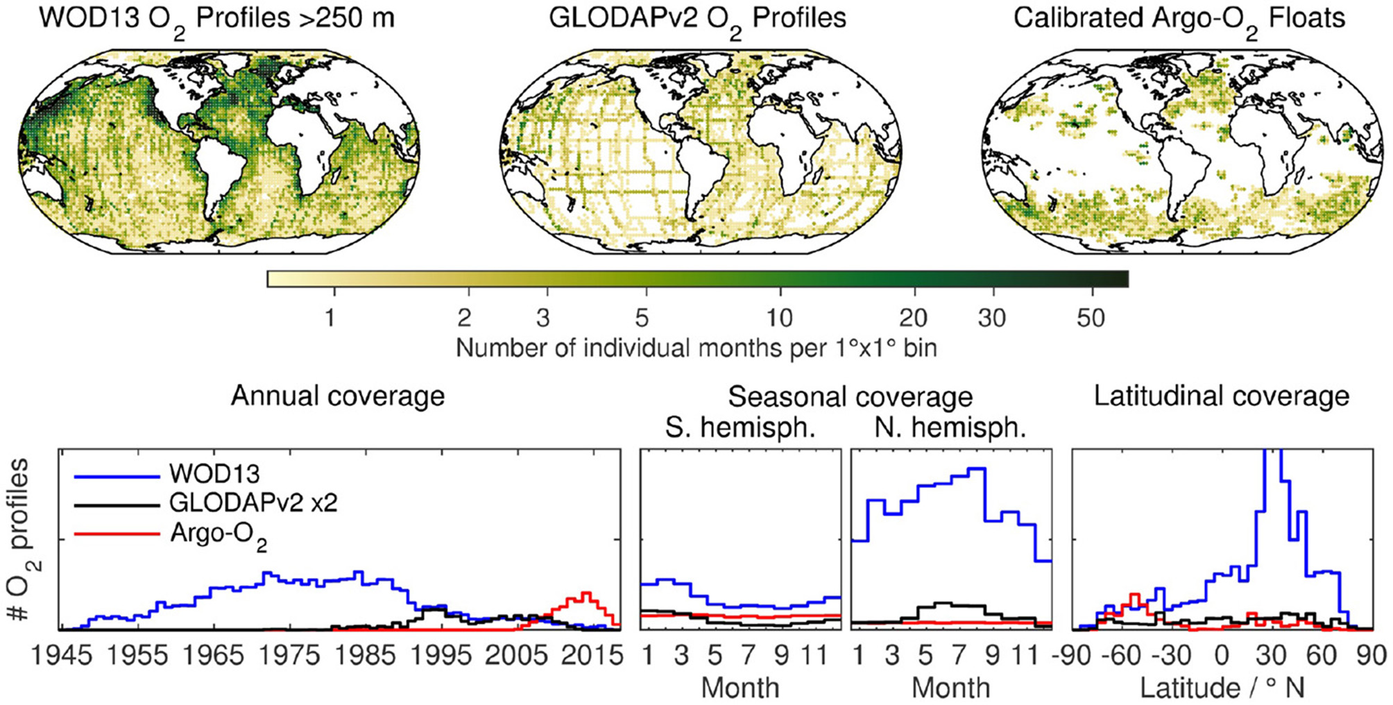
Spatial and temporal coverage of quality-controlled O2 profiles built from Argo-O2 profiles and hydrographic stations. (Top): Number of months covered by float-based or shipboard observations (assembled in GLODAPv2 or in WOD13, only using stations deeper than 250 m) for the entire period since 1945 per 1° x 1° bin. (Bottom, left to right): Annual, seasonal, and latitudinal distribution of profiles from all three sources (55 623 Argo-O2, 31 980 GLODAPv2 O2, and 383 465 WOD13 O2 profiles). The number of GLODAPv2 O2 profiles has been multiplied by a factor of 2 for visibility.
There is a need to circumvent such observational gaps, and multiple efforts are dedicated to improve the geographical, vertical, and temporal coverage of carbonate data. However, it is unlikely that discrete sampling will increase considerably considering the cost of ship time and the size and remoteness of areas that are undersampled. Autonomous platforms such as gliders and profiling floats have great potential and are increasing in numbers but, to date, only pH can be measured on those platforms operationally (Johnson et al., 2016). AT derived from empirical relationships with salinity (S), temperature (T), oxygen (O2), pressure (P), and location (e.g., Carter et al., 2018) can serve as the second variable required to resolve the carbonate system (e.g., Williams et al., 2017). Other approaches have used multiple linear regression models to determine relevant variables (e.g., Juranek et al., 2009, 2011) and to derive surface ocean pH (e.g., Lauvset et al., 2015). However, such methods have a domain of application that is restricted geographically, vertically, or in variable-space.
Here we build on the CANYON (CArbonate system and Nutrients concentration from hYdrological properties and Oxygen using a Neural-network) approach of Sauzède et al. (2017), and re-develop, based on GLODAPv2 data, more robust neural networks, “CANYON-B,” that include a local uncertainty estimate as key element. Contrary to common views of data based on temporal or spatial interpolation (e.g., for climatologies, Lauvset et al., 2016), the work presented here takes a variable-interrelation view. It thus provides mappings from one set of variables (i.e., temperature, salinity, oxygen, pressure, location, and time), which are easy to measure autonomously and accurately, to another set of variables (e.g., nitrate, phosphate, silicate, or the four carbonate system variables AT, CT, pH, and pCO2), which are more difficult or expensive to measure. Implicitly, water mass properties, biogeochemical relations, and their regional anomalies are incorporated into the neural network mappings. From the same inputs, CANYON-B provides all four carbonate system variables at once, including a local error estimate for each parameter.
We develop a second method, CONTENT, which combines all four carbonate system variables to give a consistent state of the carbonate system, i.e., the four variables jointly agree with carbonate chemistry. Using carbonate system calculations within the overdetermined system, we improve accuracy for each individual variable, and add a contribution to the local uncertainty estimate based on the consistency of these calculations.
We validate CANYON-B and CONTENT against bottle data from both a GLODAPv2 subset not used for neural network development and recent GO-SHIP cruises not included in GLODAPv2, as well as against Argo profiles of sensor data for pCO2 and pH. Moreover, we explore the boundaries of such mappings by discussing surface pCO2 estimates compared to 6 underway pCO2 cruises where calibrated O2 data were available, and surface pCO2 derived from profiling float pH data, as well as surface seasonality. Finally, the potential of such mappings is explored (1) by illustrating how they can be used to combine different observing systems on the global scale, e.g., using O2 data collections from the World Ocean Database (WOD13, Boyer et al., 2013; accessed Mar 6, 2018), GLODAPv2 or Argo to complement SOCAT data, (2) by showing how they can serve as transfer functions and go beyond existing data, e.g., for carbon variable densification or to estimate realistic depth profiles of pCO2 from solely Argo-O2 data, and (3) by demonstrating the potential of giving access to the full carbonate system, in order to easily derive ocean carbonate chemistry like the global distribution of the Revelle factor based on observations.
The same CANYON-B approach is used to develop robust mappings for the inorganic macronutrients nitrate, phosphate, and silicate [hereafter or simply NO3, or simply PO4, and Si(OH)4]. The macronutrients are essential for oceanic primary production (Falkowski et al., 1998) and limit phytoplankton growth in large parts of the ocean (Moore et al., 2013). Their distribution is governed by the interplay of physical (e.g., horizontal advection or mixing) and biological processes (nutrient assimilation at the surface and remineralization at depth), and can be used to infer information about the biological carbon pump through its correlation with new production and nutrient limitation (e.g., Koeve, 2001). However, nutrient observations are still mostly relying on research cruise bottle data and thus limited and expensive to acquire. A commercial sensor that can be mounted on robotic platforms exists only for nitrate (e.g., Johnson et al., 2013), and even then reference data or mappings as presented here are required to calibrate its data (Johnson et al., 2017). The estimation of nutrient distributions including robust, local uncertainties through, e.g., CANYON-B, thus remains of strong interest to assess nutrient supply mechanisms, biogeochemical cycling, or impacts of climate change. However, the remainder of this manuscript focusses on the carbonate system. The CANYON-B approach for NO3, PO4, and Si(OH)4 is nonetheless as thoroughly validated as for the four carbonate system variables. Corresponding Matlab and R code are available at https://github.com/HCBScienceProducts/.
Data and methods
CANYON-B to provide robust variable estimates with an appropriate local uncertainty
CANYON yields estimates of macronutrient concentrations [, , Si(OH)4], AT, CT, pHT, and pCO2 as a function of simple input variables (P, T, S, O2, latitude, longitude, and the day of the year, as well as year of measurement for CT, pHT, and pCO2 to account for the anthropogenic perturbation). In CANYON, a single neural network estimates each variable and the variable's uncertainty is based on a unique, globally uniform value derived from the validation data set.
Plain feed-forward neural networks such as used for CANYON are often “incapable of correctly assessing the uncertainty in the training data and so make overly confident decisions about the prediction” (Blundell et al., 2015). Moreover, the globally constant uncertainty does not reflect reality. Uncertainty likely differs between deep ocean and surface predictions due to the intrinsically different variability. To overcome this and other shortcomings, we used a Bayesian approach to develop new neural network mappings (i.e., “CANYON-B”), modified the training approach, and improved the uncertainty estimation.
Training modifications from CANYON
The input normalizations of longitude used trigonometric functions, sin(lon) and cos(lon), to account for the circular globe (Sauzède et al., 2017). There were two unwelcome effects, (1) a change of 1° E/W had a different magnitude depending on longitude as the gradient of sine/cosine is not constant, and (2) in the vicinity of the maxima and minima of sine/cosine, the sin(lon)/cos(lon) input lost all their explanatory potential as the gradient approached zero. These nodes were located at 0°, 90° E, 180°, and 90° W, matching Eastern boundary systems in the South Atlantic (e.g., Benguela current) as well as the South Pacific (e.g., Humboldt current) and transected the central/Eastern Pacific and Indian ocean. We changed the input normalizations to
which displays a steady gradient at all longitudes but for the single-point nodes, which are moved to 20° E, 110° E, 160° W, and 70° W (compare Lauvset et al., 2016) in order to coincide as much as possible with large landmasses instead of ocean basins. Moreover, the distance of Bering Strait, the separation between North Pacific and Arctic Ocean, was artificially increased to avoid too similar a representation in the neural networks, that is, a spill-over of information between the two basins that are only marginally connected through the very shallow Bering Strait. This was achieved by compressing the latitude input inside the Arctic for all locations west of the Lomonosov Ridge in the Amerasian and Canada basin. The “length” of Bering Strait was thus increased from ~2° to 11°. These modifications helped to give a more equal influence to the lon inputs (following Bach et al., 2015; data not shown) and to improve predictions in the subploar North Pacific.
The day of the year was removed as an input variable, as the underlying GLODAPv2 bottle data are not adequately seasonally resolved in most areas. In regions where seasonal resolution and variations exist, they can be represented by other, co-varying inputs such as temperature. In addition, we use a decimal year as year input for the CO2 variables (01 Jul. 2005 is 2005.5), whereas CANYON used only an integer year causing Jan. 2005 and Dec. 2005 to be more similar than Dec. 2005 and Jan. 2006.
Finally, we adopted a stepwise training approach: Each network topology was first trained on a climatological dataset (Lauvset et al., 2016) and then on GLODAPv2. The weights of the climatological networks were used to initialize the weights for the subsequent networks. This provides adequate starting points for the network training on the potentially scarcely distributed bottle data in multidimensional variable space. As the climatology covers a large portion of the domain on which CANYON-B is used, this stepwise procedure should avoid unreasonable predictions.
Carter et al. (2018) discuss changes in ocean pH measurement practices over time (pH calculated from AT and CT, spectrophotometric pH measurements with impure or purified dyes) that led to inhomogeneities in pH data compilations. They applied a range of corrections and thus created the most consistent pH data product presently available. We therefore use their data product for training. Note that for CANYON-B the pH data product was adjusted to be in line with pH calculations from AT and CT (Carter et al., 2018). As in Sauzède et al. (2017), pCO2 was calculated from AT and CT.
Otherwise we follow a similar approach as for CANYON: Networks are fully connected feed-forward multi-layer perceptrons, consisting of two hidden layers with tanh activation functions and one linear output layer. We systematically tested network topologies up to 60 neurons in total, with the number of neurons in the second layer not exceeding the first layer, and with a maximum of 45 neurons in the first layer. 20% of the data were set aside for validation and the remaining 80% used for training. A split of this 80% into learning or testing set (and re-shuffling for the next training epoch) for cross-validation was no longer needed (see below). Training of the neural networks was done using the Adam optimizer with variable learning rate (Kingma and Ba, 2014). Individual networks were assessed and combined into an ensemble as described below.
Bayesian neural network framework for CANYON-B
A Bayesian treatment introduces probability distributions instead of single, fixed values at all stages of a model, i.e., neural network weights, regularization parameters, but also input and output variables (Bishop, 1995; MacKay, 1995). This comes at the expense of computational cost, which has become tractable thanks to variational approximations and sampling methods that avoid the need to always treat and integrate over the full distributions (e.g., Hinton et al., 2012; Blundell et al., 2015; Wen et al., 2018).
Advantages of a Bayesian approach are that (1) regularization (balance between accuracy and overfitting) comes naturally, (2) the values of regularization coefficients can be selected using only the training data without the need for cross-validation, (3) confidence intervals can be assigned to the predictions of a network, and (4) different models can be compared and assigned a “model evidence” using only the training data (from Bishop, 1995). This allows objective comparison between networks and network architectures, penalizing overly flexible and overly complex models (“Occam's razor”) (e.g., MacKay, 1992a,b).
The output of a Bayesian neural network comes with a “most-probable” value and an uncertainty on this value. Applying the Bayesian approach on a higher level, several neural networks can be combined to build a “committee of neural networks”. Committees have the advantage of showing improved generalization behavior and that the spread of predictions between members of the committee provides a contribution to the estimated prediction uncertainty in addition to those identified already, leading to more accurate estimation of uncertainty (Bishop, 1995).
For CANYON-B, we use the evidence to build a committee as a weighted average of networks with output yC and yi's, respectively,
where wEvi are the respective weights based on the networks' evidences (Thodberg, 1996). We used the models with the highest evidence for the committee and stopped the series at the network with weight wEvN+1, which would contribute less than 2% to the total weighted sum. N varies between 22 (for AT) and 33 individual networks (for NO3).
CANYON-B local uncertainty estimation
Training of an individual Bayesian neural network provides one uncertainty estimate with a contribution from the intrinsic noise of the target data, σnoisei, and one arising from the distributions of the network weights and their respective weight uncertainty, σWUi. Both are weighted following Equation (2) to yield σnoise and σWU, respectively. The weighted standard deviation of the committee mean,
provides the committee uncertainty, σCU, which together with σnoise and σWU yield the Bayesian neural network uncertainty, σNN:
The estimated CANYON-B output uncertainty then is
where σmeas is the measurement uncertainty of the respective data product used for training. We use 6 μmol kg−1 AT, 4 μmol kg−1 CT, 0.005 pH, 2% , 2% , and 2% Si(OH)4 (Olsen et al., 2016). For pCO2, σmeas follows the calculation uncertainty of pCO2 from AT and CT (ca. 5% pCO2). For pH, we follow Orr et al. (submitted manuscript) and add a systematic 0.01 pH uncertainty related to “the activity coefficient of Cl− in the buffer solutions that are used as pH standards”. Uj are the n uncertainties for the neural network inputs and αj the input sensitivities. Only the input uncertainties of pressure, temperature, salinity, and oxygen are considered (i.e., n = 4) with default uncertainties of 0.5 dbar, 0.005 °C, 0.005, and 1% of the O2 value, respectively. Note that 1% O2 is a rather optimistic value and appropriate for Winkler-based bottle samples, but probably too small for most O2 sensor data.
The calculation of the weight uncertainty σWU represents more than 90% of the CANYON-B computation time. As σWU is typically similarly distributed and of smaller magnitude than σCU, we parameterize σWU by σCU for practical purposes. Note that σCANYON−B is a local value, mostly due to σCU but also due to αj. For the nutrients, σmeas varies locally, too.
Carbonate system calculations
Thermodynamic calculations within the carbonate system used the carbonic acid dissociation constants of Lueker et al. (2000), the hydrogen fluoride dissociation constant of Pérez and Fraga (1987), the dissociation constant for bisulphate of Dickson (1990), and Uppström (1974) for the ratio of total boron to salinity. Phosphate and silicate alkalinity were included, either directly where nutrients had been measured (GLODAPv2) or indirectly through their CANYON-B estimates. These constants were used for consistency with the calculations performed in GLODAPv2 and the best practice guide for CO2 (Dickson et al., 2007). Calculations were done by CO2SYS-MATLAB v2.0 (Lewis and Wallace, 1998; van Heuven et al., 2011; Orr et al., submitted manuscript). Hydrostatic pressure effects on pCO2 solubility were neglected and pCO2 is given at 1 atm pressure and in situ temperature. The uncertainty associated with the calculations was estimated by CO2SYS-MATLAB's “errors” function (Orr et al., submitted manuscript), taking the uncertainty of the input as well as of the equilibrium constants into account (Table 1).
Table 1
| Variable | AT / μmol kg−1 | CT / μmol kg−1 | pHT | pCO2 |
|---|---|---|---|---|
| σCANYON−B | 8.8 | 8.8 | 0.018 | 8.2% (33 μatm at 400 μatm) |
| σcalculation of the indirect estimates (median uncertainty from all GLODAPv2 O2 data) |
pCO2/CT 16.3 | pCO2/AT 14.3 | AT/CT 0.034 | AT/CT 8.3% (33 μatm at 400 μatm) |
| pH/CT 11.3 | pH/AT 11.0 | pCO2/CT 0.035 | pH/AT 4.7% (19 μatm at 400 μatm) |
|
| pCO2/pH 213.8 | pCO2/pH 203.2 | pCO2/AT 0.033 | pH/CT 4.4% (18 μatm at 400 μatm) |
|
| (≤ σCONTENT) | 7.1 | 6.9 | 0.015 | 3.7% (15 μatm at 400 μatm) |
Median uncertainties of CANYON-B AT, CT, pH, and pCO2 (σCANYON−B) as well as indirect carbonate system calculations (σcalculation) for all GLODAPv2 O2 data as input.
These uncertainties are calculated point-by-point and are used for the CONTENT weights (Equation 7) and uncertainty estimation (, Equation 9). As both the uncertainty of the carbonate system pCO2 calculations as well as the uncertainty of CANYON-B pCO2 increase nearly proportionally with pCO2, we chose to provide a relative σ in % for pCO2 rather than an absolute σ in μatm.
CONTENT to ensure consistency between the carbonate system variables
With all four carbonate system variables AT, CT, pHT, as well as pCO2 available along with an estimate of their respective uncertainties, one obtains a fully characterized and overdetermined carbonate system. By comparing the direct variable estimate with the ones calculated from any two other carbonate system variables, one can refine the estimate of the given variable. This combination yields an estimate for each of the four variables that is internally consistent with the state of the CO2 system (due to the internal consistency of carbonate system calculations, Millero, 2007).
At the same time, the mismatch between the different estimates provides an indication of how consistent the carbonate system is described (details below). To highlight this duality, we call our approach CONTENT for “CONsisTency EstimatioN and amounT.”
CONTENT is a priori independent of the source of the variable estimate and could combine different observation techniques, MLRs, or neural network mappings, as well as different sets of carbonate system equilibrium constants. For the CONTENT presented here, we use CANYON-B, which provides AT, CT, pHT, and pCO2 from the same inputs along with a local estimate of their respective uncertainties, as well as the set of constants as described above.
CONTENT calculation
Here we describe the CONTENT calculation using pCO2 as the variable of interest. The calculation of CONTENT AT, CT, or pH is analogous. There is a direct pCO2 estimate and three indirect estimates calculated from the pairs AT/CT, pH/AT, and pH/CT (Figure 2). The CONTENT pCO2 estimate, , is the weighted sum of these,
where xi = pCO2,i is one of the four pCO2 estimates, either directly from CANYON-B or indirectly based on the calculations. The weights, wi, are determined from the uncertainty σi of the individual CANYON-B estimate or the calculations, respectively.
Orr et al., (submitted manuscript) provide functions that allow the on-line calculation of the CO2 calculation's uncertainty (including the uncertainty of the input variables as well as the equilibrium constants) for a suite of CO2 system calculation tools. Thus for CONTENT, σi is dependent on and reflects the local conditions both for the direct CANYON-B estimate as well as for the indirect, calculated values. Table 1 gives average values of σi for the GLODAPv2 O2 data set.
Figure 2
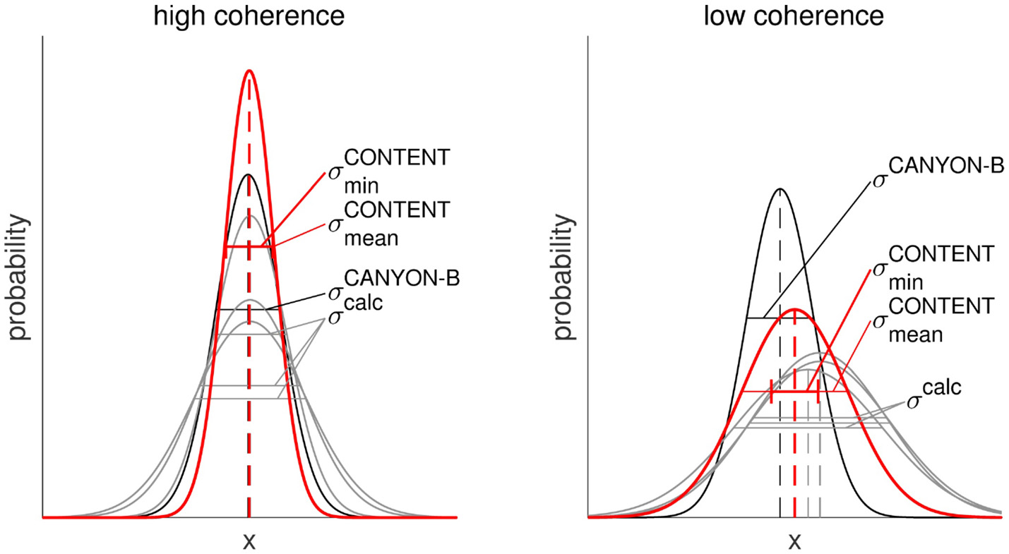
Conceptual illustration of CONTENT. For each carbonate system parameter, CANYON-B provides one direct estimate (black) and three calculated, indirect estimates (gray). (Left) The four estimates (with associated uncertainty distribution) are consistent and support each other to give the CONTENT estimate (red). The CONTENT uncertainty is smaller than any of the input uncertainties (σCONTENT ≈ ; ≈ 0). (Right) The four parameter estimates are inconsistent (centered around different values). The additional contribution to CONTENT's uncertainty by the mismatch of the four independent estimates provides an uncertainty that adjusts to the local conditions.
Since CONTENT combines four variables (from CANYON-B) with additional constraints (those of the CO2 system), its results tend to be more tightly constrained than the individual estimates (using only one CANYON-B). However, its meaning may have shifted: Whereas CANYON-B and similar mapping techniques provide a best estimate of the measured variable, CONTENT provides an estimate of the variable that is as consistent as possible with measurements of the complete carbonate system, given the constraints of today's knowledge of the carbonate system equilibrium constants.
CONTENT local uncertainty estimation
The uncertainty of the CONTENT estimate (σCONTENT; Equation 8) can be calculated from the uncertainty of the inputs to the weighted mean (i.e., of the direct CANYON-B and the three calculated estimates; see Table 1 and Equations 7, 9) and the mismatch of these four estimates with respect to their weighted mean (Equation 10):
with
and
where is the standard deviation propagated from the uncertainty of the terms of the weighted mean (Equation 6), is the standard deviation associated with the weighted mean due to disagreements, and Cov(xi, xj) is the covariance between estimate xi and xj. For i = j, Cov(xi, xj) is equal to the variance .
A priori, each of the four variable estimates is independent as each of them originates from the individual CANYON-B training and estimation for the individual variable. However, they are parameterized by the same set of inputs and, as such, correlations can exist between CANYON-B variables and also between the direct CANYON-B estimate and the three calculated, indirect estimates used for CONTENT. These correlations manifest themselves in non-zero covariance terms Cov(xi, xj) for i ≠ j. They increase by ca. 20% compared to a complete independence[i.e.,Cov(xi, xj) = 0 for i ≠ j],e.g., if independently measured datawere used.
provides an improvement by using 4 instead of just 1 estimate (Equation 9), while gives a measure of the consistency of the estimates (Equation 10). is thus a lower bound on the CONTENT uncertainty σCONTENT. If all four variable estimates give the same value, the local state of the carbonate system is described consistently by the four CANYON-B estimates. In that case, approaches zero (and σCONTENT is close to ; Figure 2, left). However, a disagreement between the four variable estimates (i.e., a large ; a σCONTENT that is much larger than ) indicates that the individually-trained CANYON-B carbon system variables do not yield a consistent state of the carbonate system (Figure 2, right). Like σCANYON−B, σCONTENT provides an uncertainty that is adapted to the local conditions, and additionally includes the carbonate system description's consistency.
CONTENT training data density indicator
Apart from σCONTENT/, a second quality marker for CONTENT is obtained from the density of the underlying GLODAPv2 training data. For any parameterization, regions with high data coverage tend to be more robustly parameterized than regions with fewer data. This holds also for the combination of neural network estimates.
As a first guess to assess the data density that went into the CONTENT estimate, we use the number of cruises in GLODAPv2 with carbonate system observations within a box of ±20° of the geolocation and within ±30 days of the respective day of the year.
The number of stations could have been used instead but distance/density of stations per cruise can vary considerably. Furthermore, adjacent stations tend to be strongly correlated, while different cruises are independent, which provide a better indicator. Other indicators are easily derivable from the GLODAPv2 dataset (Key et al., 2015; Olsen et al., 2016).
Validation and comparison data
Metrics
We use three bulk metrics that are applied on the data collections detailed below:
-
The bias, Δ, of estimated minus reference value,
-
the (local or global) uncertainty, σ, provided by the method for these conditions, and
-
the ratio between (absolute) bias, |Δ|, and uncertainty, σ, with a cutoff of 1, i.e., whether the uncertainty is adapted for the local bias.
GLODAPv2 validation data and post-GLODAPv2 GO-SHIP cruise data
We use the 20% of GLODAPv2 data set aside for validation to assess the neural network training success of CANYON-B. For pCO2, we compare the neural network results both against pCO2 calculated from AT and CT (as for the training) and against pCO2 calculated from combinations of AT, CT, and pH (as with CONTENT). The same data are used to compare CANYON-B results with CONTENT, CANYON (Sauzède et al., 2017), and LIR (locally interpolated regressions, Carter et al., 2018) results. They are assessed by the metrics above. For LIR and CANYON, part of the 20% CANYON-B validation data may have been used for training/algorithm development so their results might be too optimistic, but we believe them to be nonetheless in a realistic range.
Since the completion of the GLODAPv2 collection, a number of GO-SHIP repeat hydrography cruises were completed. Their data are likely of as high a quality as possible (albeit not yet made internally consistent) and they provide a completely independent validation set. As pCO2 is not a measured variable, it was calculated from the combinations of AT, CT, and pH to arrive at the most likely value of pCO2 given carbonate system constraints (i.e., comparable to the CONTENT approach). In total, this validation set encompasses 19 cruises between 2012 and 2017 that cover all ocean basins. As part of these cruises has been included in the pH dataset of Carter et al. (2018), only the 6 more recent cruises (18MF20120601, 29AH20120622, 320620170703, 320620170820, 49NZ20121128, 49NZ20130106) were used for the pH comparison. Cruise 49NZ20111220 was excluded as there seems to be a low pH bias (order of −0.020 to −0.015).
Surface underway observations of pCO2
While surface underway observations of pCO2 (by research or voluntary observing ships) are comparatively abundant and feed the majority of the data compiled in SOCAT unfortunately only very few obtain O2 data of high accuracy in parallel. This hinders a direct comparison of surface pCO2 estimates with pCO2 data on a global scale, so that we had to limit our comparison to the six cruises described below.
As part of the OCEANET project, surface underway measurements of several dissolved gases were performed onboard R/V Polarstern on six transects across the Atlantic Ocean in spring and autumn between 2008 and 2010. Cruises were either between Bremerhaven/Germany and Capetown/South Africa (ANT-XXV/1, ANT-XXVII/1) or Bremerhaven/Germany and Punta Arenas/Chile (ANT-XXIV/4, ANT-XXV/5, ANT-XXVI/1, and ANT-XXVI/4), with Apr./May cruises heading north and Oct./Nov. cruises heading south.
Surface O2 was measured using a fully submerged oxygen optode (Aanderaa Data Instruments AS, Bergen, Norway; models 3830 or 3835) in a thermally insulated flow-through box (50 or 80 L volume). Seawater was continuously pumped through the box from the ship's keel intake (at 11 dbar) with a flow rate of ~12 L min−1. Optodes were laboratory multi-point calibrated and sensor drift between deployments was checked against in-situ bottle observations.
The pCO2 measurements were done using different instruments, all of them following the same principle where water is led through a gas-water equilibrator with subsequent measurement of the xCO2 in the dried, seawater-equilibrated air. During all cruises, an infrared sensor was used for CO2 detection (either LI-6262 or LI-7000, LI-COR Biosciences, Lincoln, NE) which was calibrated every 3–4 h using three non-zero standard gases between 200 and 700 ppm, traceable to WMO scale. After each calibration run, atmospheric air was measured for ~10 min. The sea surface temperature (SST) and sea surface salinity (SSS) were recorded by the ship's thermosalinograph (SBE21, Seabird, Bellevue, WA). Atmospheric pressure was taken from the ship's weather station that is maintained by the German weather service. The data reduction for all cruises included the correction to SST and was done following the recommendations given in Dickson et al. (2007) and Pierrot et al. (2009). As an additional reference, discrete water samples were taken up to four times a day during all cruises. The samples were analyzed for CT and AT in the laboratory at GEOMAR, Kiel.
For the first cruise, ANTXXIV/4, water was pumped to the instruments using the ships rotary pump (installed at a depth of 11 m). A custom-built underway pCO2 system with a combined laminar flow/bubble equilibrator was used, which is described in detail in Körtzinger et al. (1996). The resulting accuracy was estimated to be ±3 μatm.
For the second cruise, ANTXXV/1, water was drawn from two different inlet points (5 and 11 m) using a membrane pump. The infrared analyzer was coupled to a small (0.5 L) equilibrator. Due to the different inlets and resulting different intake temperatures, the dataset was treated carefully for the different settings. The resulting accuracy is ±5 μatm.
For the remaining cruises, ANTXXV/5 – ANTXXII/1, water was pumped to the instruments using the ships rotary pump (installed at a depth of 11 m). A commercially available pCO2 instrument was used (GO, General Oceanics, Miami, FL) which uses a shower head equilibrator and is described in Pierrot et al. (2009). The resulting accuracy was estimated to be ±2 μatm.
pCO2/O2 profiling float observations
To date, only one experimental Argo-type float was deployed with a pCO2 sensor (Fiedler et al., 2013), so opportunities for an on-platform, depth profile validation of pCO2 are very limited. Nonetheless, this float provides a unique data set since it was recovered and redeployed several times, thus providing insight into sensor drift thereby allowing drift and other corrections.
A HydroC pCO2 sensor (Kongsberg Maritime Contros GmbH, Kiel, Germany) and a battery/buoyancy container were mounted on the float's side. Profile data were acquired on the float's ascent. Details about the float, the pCO2 sensor, and data treatment can be found in Fiedler et al. (2013) and Fietzek et al. (2013), respectively. In addition, its O2 optode data were recalculated according to most recent knowledge, including drift behavior, pressure compensation, response time correction, and in-air calibration (Bittig et al., 2018). The float was deployed four times (D4–D7) between Nov. 2010 and Jun. 2011 near the Cape Verde Ocean Observatory (CVOO) in the eastern tropical North Atlantic. It performed a total of 123 profiles (111 with pCO2 data) between 200 dbar and the surface.
The float was lost and could not be recovered at the end of deployment D7, which means that only low-resolution HydroC data transmitted by satellite are available. This limits the potential of post-correction of the pCO2 data, notably the sensor's time lag correction (see Fiedler et al., 2013, for details), and so we group D4 – D6 separately from D7.
Fiedler et al. (2013) give a sensor accuracy for profile data of 10–15 μatm when compared to pCO2 calculated from in-situ samples of CT and AT in areas of low gradients.
pH/O2 profiling float observations
At present, ISFET-based pH sensors (Johnson et al., 2016) are the only operationally available carbonate system sensors that can be used on floats. Such observations provide important insight into the state of the carbonate system. As part of the SOCCOM (Southern Ocean Carbon and Climate Observations and Modeling) project, several BGC-Argo floats with pH sensors were deployed in the Southern Ocean (e.g., Johnson et al., 2017). Williams et al. (2017) used data from these floats in combination with an MLR-based estimate of AT to estimate surface pCO2 in the Southern Ocean with a relative standard uncertainty of 2.7% (11 at 400 μatm). The floats used are WMO 5904395 in the South Pacific subtropical zone, 5904396 in the South Pacific subantarctic zone, 5904469 in the South Atlantic polar antarctic zone, and 5904468 in the South Atlantic seasonal sea ice zone (see Figure 7 for float location).
Transfer data set of quality-controlled O2 profiles
Quality-controlled and calibrated data of O2 profile data were compiled using both shipboard hydrographic stations (WOD13 and GLODAPv2) as well as Argo-O2 profiles accessed from various sources. WOD13 data are Northern hemisphere- and coastal ocean-focused, while GLODAPv2 O2 profiles have a globally balanced distribution (Figure 1). Ship-based observations cover mostly the decades before 2010, and are strongly biased toward summer in both hemispheres while Argo-O2 float data have a focus on the Southern Ocean and the subpolar North Atlantic. They are mostly limited to the last decade and they are seasonally unbiased.
In order to exclude coastal/shelf stations we used all O2 profiles from WOD13 after Jan 1, 1945 that sampled to at least a depth of 250 m. Data were additionally quality controlled for reasonable ranges of T, S, and O2, which leaves a total of 383 465 profiles between Sep 4, 1945, and Apr 21, 2017.
From GLODAPv2, only those data were used where salinity and oxygen had both a good primary QC (WOCE-type flag 2 meaning “acceptable”) as well as where they had been made internally consistent by a crossover analysis (secondary QC flag 1). In the Mediterranean, only one zonal repeat hydrography section exists that does not intersect with any other sections, which prevents a crossover analysis there. Therefore, the second condition was relaxed (secondary QC flag 0) for the two cruises in GLODAPv2 across the Mediterranean. Moreover, there had to be at least 5 samples per profile. These criteria matched to 31 980 profiles from 521 cruises between Jul. 24, 1972, and May 20, 2013.
For Argo, a total of 262 floats with adjusted and quality controlled O2 data were obtained from the Argo Global Data Assembly Centre (GDAC) at Coriolis (ftp.ifremer.fr/ifremer/argo/) on May 15, 2018 (Argo, 2000). They encompass 38 622 CTD-O2 profiles between Feb. 24, 2005, and May 14, 2018. In addition, calibrated data of 84 Argo-O2 floats deployed by the University of Washington (http://runt.ocean.washington.edu/o2/) were included in the transfer data set. This excludes floats with a calibration accuracy estimate larger than 5 μmol kg−1 as well as floats covered by SOCCOM, which are already included in the GDAC data. This adds a total of 14 347 profiles between Oct. 26, 2005, and Aug. 24, 2015. Moreover, data from 2 floats consisting of 401 calibrated O2 profiles between Sep. 27, 2013 and Dec. 6, 2016, (see Bittig and Körtzinger, 2017) as well as from 12 floats deployed as part of the remOcean project with 2 253 profiles (Oct. 24, 2012–Apr. 13, 2018) were added. The Argo-O2 data set contains 360 individual floats with 55 623 calibrated profiles (Feb. 24, 2005–May 14, 2018) with global coverage and a focus on the Southern Ocean and the North Atlantic.
For comparison, there are 13 916 profiles with concurrent AT and CT observations in GLODAPv2 within the three decades it covers. The GLODAPv2 O2 data set encompasses 31 980 profiles for the same period, which represents already a densification by a factor of 2.3. The complete transfer data set contains about 470 000 O2 profiles distributed over 7 decades, i.e., an average densification by a factor of 15. The number of GLODAPv2 NO3 profiles is 27 277, i.e., the transfer data set represents a densification of 7.4.
Revelle factor R
The Revelle factor, R, characterizes the capacity of the carbonate system to take up more CO2. In detail, it relates the relative change in pCO2 to the associated relative change in CT.
Egleston et al. (2010) provide an explicit formula to calculate R from the state of the carbonate system, given by the combination of any two carbonate system variables. A higher R means that a larger change in pCO2 is needed to actually result in a respective change in the ocean's carbon content CT, i.e., the oceans CO2 uptake capacity is lower.
With CONTENT, we can derive CT and AT from any Argo-O2 profile or any other set of CTD-O2 data, thus largely expanding the number of R estimates compared to using carbonate system data alone.
Dataset results and analysis
Intercomparability of CANYON/CANYON-B/CONTENT/LIR
Table 2 gives a summary of the performance of CANYON, CANYON-B, CONTENT, and LIR on the combined 20% GLODAPv2 validation bottle data and the post-training/-GLODAPv2 cruise bottle data (see section Assessment of CANYON-B and CONTENT for detailed results). The metrics shown here can be used as global average statistics.
Table 2
| Variable | Method | Bias Δ | Bias Δ | Uncertainty σ | |Δ| > σ / % |
|---|---|---|---|---|---|
| rmse | 10 / 50 / 90th | 10 / 50 / 90th | – / + / ∑ | ||
| NO3 / μmol kg−1 | CANYON | 0.93 | −0.82 / −0.02 / +0.80 | 0.95 / 1.10 / 1.21 | 6.8 / 6.8 / 13.6 |
| CANYON-B | 0.68 | −0.55 / +0.00 / +0.57 | 0.82 / 0.99 / 1.11 | 3.9 / 4.2 / 8.2 | |
| LIR | 0.84 | −0.58 / +0.00 / +0.63 | 1.07 / 1.32 / 1.36 | 3.0 / 3.7 / 6.7 | |
| PO4 / μmol kg−1 | CANYON | 0.066 | −0.060 / +0.002 / +0.066 | 0.068 / 0.078 / 0.086 | 7.1 / 8.1 / 15.2 |
| CANYON-B | 0.051 | −0.044 / +0.002 / +0.052 | 0.059 / 0.071 / 0.080 | 4.6 / 5.9 / 10.5 | |
| Si(OH)4 / μmol kg−1 | CANYON | 3.4 | −2.7 / +0.3 / +3.3 | 3.0 / 3.2 / 4.3 | 6.8 / 8.6 / 15.4 |
| CANYON-B | 2.3 | −1.9 / +0.1 / +2.0 | 2.4 / 2.8 / 3.9 | 4.4 / 4.2 / 8.5 | |
| AT/ μmol kg−1 | CANYON | 7.3 | −5.9 / +0.3 / +6.5 | 9.5 / 9.5 / 9.6 | 3.7 / 4.4 / 8.0 |
| CANYON-B | 6.3 | −4.7 / +0.2 / +4.9 | 8.7 / 8.9 / 9.3 | 2.4 / 2.3 / 4.7 | |
| CONTENT | 6.2 | −5.5 / −0.5 / +4.1 | 7.9 / 9.3 / 12.3 | 2.5 / 1.4 / 3.9 | |
| LIR | 9.9 | −5.5 / +0.6 / +6.6 | 4.5 / 6.0 / 8.8 | 9.1 / 11.2 / 20.3 | |
| CT/ μmol kg−1 | CANYON | 9.0 | −7.8 / −0.2 / +7.2 | 11.3 / 11.3 / 11.4 | 5.2 / 4.8 / 10.0 |
| CANYON-B | 7.1 | −6.0 / −0.2 / +5.0 | 8.6 / 8.8 / 10.3 | 3.7 / 3.3 / 7.0 | |
| CONTENT | 6.9 | −4.7 / +0.6 / +5.9 | 7.7 / 9.1 / 11.8 | 2.6 / 3.3 / 6.0 | |
| pH | CANYON* | 0.019 | −0.011 / +0.006 / +0.023 | 0.022 / 0.022 / 0.022 | 3.5 / 11.2 / 14.7 |
| CANYON-B | 0.013 | −0.012 / −0.000 / +0.012 | 0.018 / 0.018 / 0.019 | 3.8 / 4.5 / 8.3 | |
| CONTENT | 0.013 | −0.009 / +0.002 / +0.015 | 0.017 / 0.019 / 0.023 | 2.5 / 5.4 / 7.9 | |
| LIR | 0.016 | −0.016 / −0.003 / +0.013 | 0.015 / 0.020 / 0.021 | 7.0 / 5.6 / 12.6 | |
| pCO2f(CT,AT,pH)/ μatm | CANYON | 23 | −29 / −6 / +13 | 30 / 40 / 70 | 3.9 / 1.3 / 5.1 |
| CANYON-B | 20 | −24 / −4 / +10 | 29 / 41 / 81 | 1.9 / 0.6 / 2.4 | |
| CONTENT | 15 | −14 / +1 / +14 | 17 / 22 / 40 | 3.5 / 3.4 / 6.8 |
Global statistics of the performance of CANYON (Sauzède et al., 2017), CANYON-B, CONTENT, and LIR (Carter et al., 2018; version 2.0.1) on the combined 20% validation GLODAPv2 bottle data and the post-training/-GLODAPv2 cruise bottle data: Bias Δ with root-mean-square error (rmse) as well as 10/50/90th percentiles, estimated uncertainty σ with 10/50/90th percentiles, and fraction of bias exceeding uncertainty in % for underestimation, overestimation, and the sum of both (– / + / ∑), respectively.
CANYON pH was trained on a not homogenized pH data set.
It should be stressed that similar global (bulk) statistics between methods do not imply that they give the same result. E.g., the NO3 bias for CANYON-B and LIR, or the AT bias for CANYON and LIR show almost identical distribution (Table 2, Figure 4). Nonetheless, the difference between both estimates has a root-mean-square error (rmse) of 0.53 μmol kg−1 NO3 and 8.7 μmol kg−1 AT. This is in the same order of magnitude as the rmse of the bias Δ to the reference data, i.e., global bulk statistics can be the same, but their estimates still are quite different, which is important to consider when choosing a particular estimation method. If there is no particular reason to favor a given method, it is probably wise to average different approaches, e.g., a neural network mapping (CANYON-B or CONTENT) with a regression method (e.g., LIR).
Assessment of CANYON-B and CONTENT
GLODAPv2 and post-GLODAPv2 validation data to assess training success and generalization skill
The distributions of Δ, σ, and the fraction where |Δ| > σ that resulted from the comparison with the GLODAPv2 validation data set are given in Figure 3 against depth for each of the 7 CANYON-B variables [NO3, PO4, Si(OH)4, pCO2, AT, CT, and pH] with their median as well as 10/90th percentiles. For pCO2, we give the distribution against pCO2 calculated from AT and CT (48 k samples) as well as against pCO2 calculated from the combination of AT, CT, and concurrent pH where available (9.5 k samples for the validation set) to account for the conceptual difference between CANYON-B and CONTENT. Apart from pH, biases are in general comparable between all methods, i.e., their median is close to zero and 10/90th percentiles are of similar size. The percentiles of CANYON-B are slightly smaller than those for CANYON. In addition, CANYON CT seems to have a small negative bias in deep waters. For all variables but pCO2, CANYON-B has a lower uncertainty σ than CANYON as well as a smaller fraction of bias exceeding uncertainty, resulting from a better co-location of high/low uncertainties with high/low biases. In particular, the increase in bias toward the surface (upper 500–1,000 dbar) seen for all methods is accompanied by a higher local uncertainty for CANYON-B and CONTENT, leading to a smaller exceedance fraction compared to CANYON. In addition, CANYON Si(OH)4 shows a considerable increase in |Δ| > σ in intermediate waters, i.e., a higher fraction of data with high bias that is not accompanied by an elevated uncertainty. LIR estimates of NO3, pH, and AT show a comparable bias to CANYON-B and CONTENT. However, their uncertainty is of a different character and shows a stronger decrease with depth. For NO3, LIR uncertainties are higher than CANYON-B uncertainties above 4,000 dbar, while for pH they intersect around 1,500 dbar. Except for very deep pH (>4,000 dbar), the two methods show a comparable |Δ| > σ distribution for NO3 and pH. However, LIR AT uncertainties are with up to a factor of 2 smaller than CANYON-B or CONTENT uncertainties below 2,000 dbar. This comes at the cost of a fraction |Δ| > σ that is an order of magnitude higher for LIR AT. Finally, the bias of pCO2 calculated from AT and CT is smallest for CANYON-B and CANYON estimates, while CONTENT estimates match pCO2 calculated from the combination of AT, CT, and pH. In both cases, predicted CONTENT pCO2 uncertainties are about half the CANYON-B and CANYON uncertainties. At the same time, the fraction of |Δ| > σ associated with the smaller CONTENT pCO2 σ is about an order of magnitude higher than their CANYON-B and CANYON counterparts for the pCO2 = f(AT, CT) validation set, which is reduced to about a factor of 5 higher for the pCO2 = f(AT, CT, pH) validation set.
Figure 3
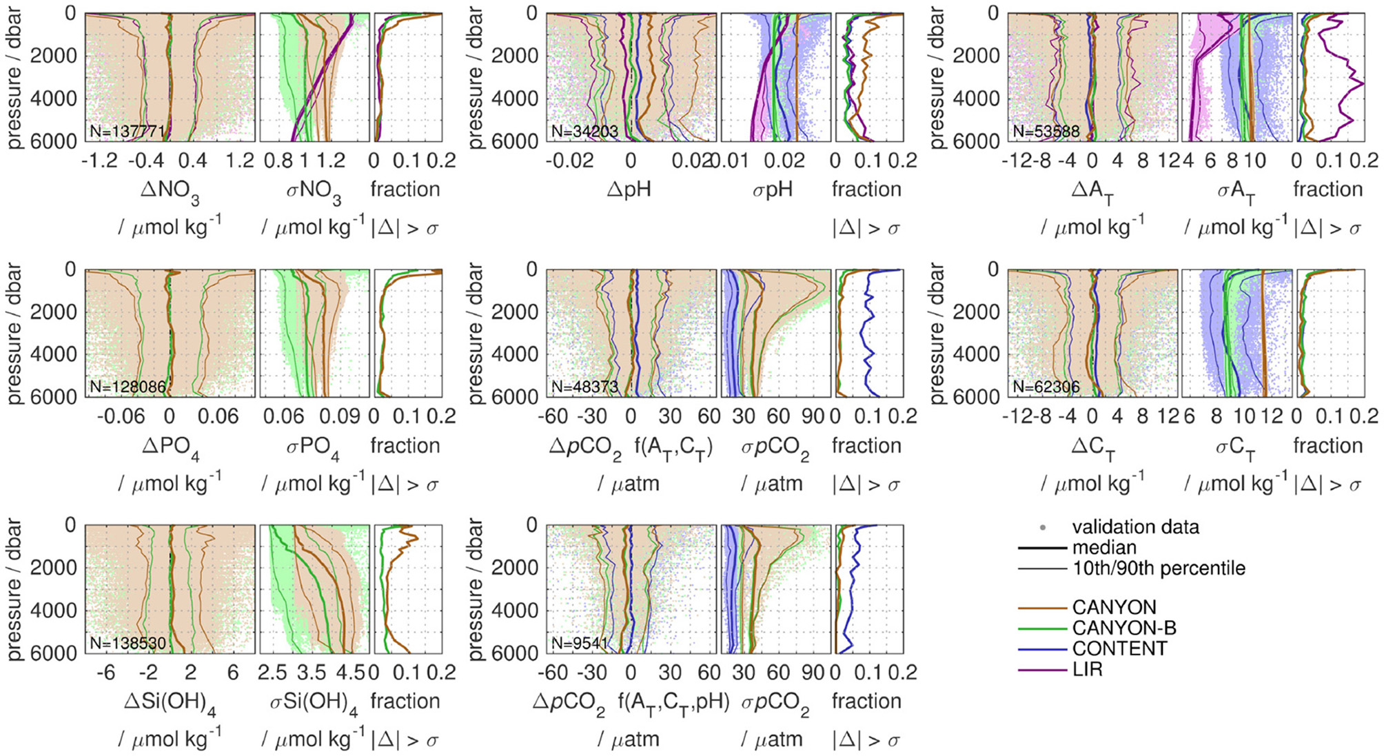
Performance of CANYON (brown), CANYON-B (green), CONTENT (blue), and LIR (purple) on the GLODAPv2 validation data set of the CANYON-B training. Panels for each variable give the bias Δ to validation data, the estimated uncertainty σ, and the fraction of bias exceeding uncertainty against depth. Thick lines give the median, thin lines the 10/90th percentiles, and pale-colored dots the data. There are two panels for pCO2, one for comparison against pCO2 calculated from measured AT and CT, and one for pCO2 calculated from the combination of AT, CT, and pH. Estimates between methods are unbiased (but for pH) and mostly differ in their uncertainty estimate and whether the uncertainty is appropriate under the given conditions (ratio Δ to σ).
As a second, independent data set we use data from those recent GO-SHIP cruises that have not been included in the GLODAPv2- or Carter et al. (2018)-based training data. Since most of these cruises measured AT, CT, and pH, the reference pCO2 has been calculated from their combination and thus reflects the most likely pCO2 derived from internally consistent carbonate system calculations (Figure 4). The nutrient estimates for CANYON-B, CANYON, and LIR (only NO3) are unbiased, while CANYON-B shows the smallest standard deviation in Δ. In addition, predicted σ is smallest for CANYON-B, and CANYON-B and LIR show the smallest fraction of |Δ| > σ. Estimates of AT, CT, and pH are unbiased for all methods except for CANYON pH, as the training data were a mixture of calculated and spectrophotometric pH. At the same time CONTENT biases show the smallest standard deviation, followed by CANYON-B. The uncertainty distribution of CONTENT is considerably wider (i.e., less peaked) than for CANYON-B or CANYON, and CANYON-B and CONTENT shows a smaller predicted σ than CANYON. At the same time, CONTENT shows the smallest |Δ| > σ fraction, followed by CANYON-B, with an improvement of at least a factor of 2 compared to CANYON. LIR's pH uncertainty estimation is comparable to CONTENT's, however, LIR shows a twice as high fraction of |Δ| > σ. LIR's AT uncertainty, in contrast, is considerably smaller than for all other methods, but at the same time the fraction of bias exceeding uncertainty is almost an order of magnitude higher. pCO2 estimates from CANYON and CANYON-B (based on calculations from AT and CT) are slightly biased low by −9 and −7 μatm, respectively, while CONTENT is unbiased to reference pCO2 (calculated from the combinations of AT, CT, and pH) and shows the smallest standard deviation in Δ. The pCO2 uncertainty estimate of CONTENT is about half the size of CANYON-B's or CANYON's (median 23 vs. 43 and 42 μatm, respectively). While CANYON-B shows the smallest fraction of Δ > σ, CONTENT's halved σ elevates its |Δ| > σ fraction only by a small amount (factor 2 or 2%).
Figure 4
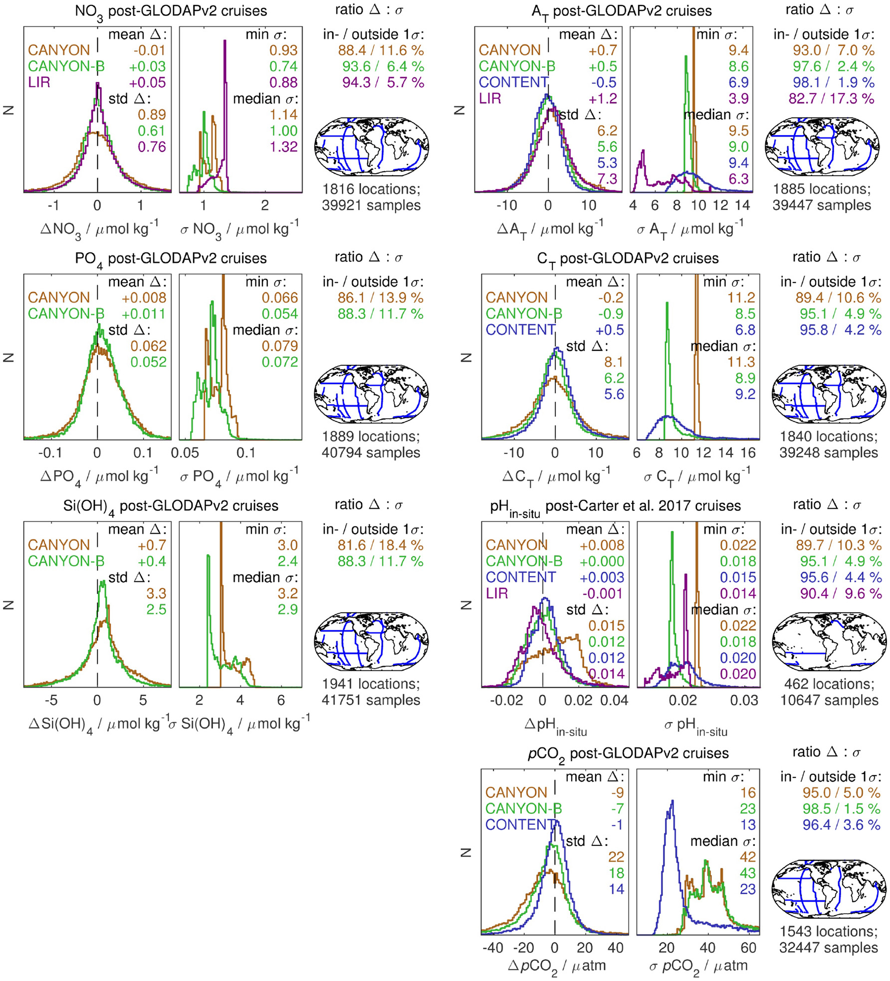
Performance of CANYON (brown), CANYON-B (green), CONTENT (blue), and LIR (purple) on recent GO-SHIP data that have not been part of the GLODAPv2 training, for NO3, PO4, SiOH4 (left column) and AT, CT, pH, and pCO2 (right column). pH data have been converted to be consistent with “calculated pH” (see Carter et al., 2018) and pCO2 was calculated from the combination of AT, CT, and pH. Left panels show the bias Δ distribution (with statistics), right panels the uncertainty σ distribution (with statistics), and the map the spatial data distribution.
Generally the CANYON-B neural networks are more robust than their CANYON counterparts. This is not entirely surprising, as CANYON-B uses an ensemble of neural networks for each variable (compared to a single “best-performing” one for CANYON) as well as other techniques to better assess uncertainty of the models (Blundell et al., 2015; Gal and Ghahramani, 2016). Their bulk mean biases are comparable and close to zero. The crucial difference lies in (1) in a higher fraction of correct estimates in the right place and (2) better knowing when this may not be the case, i.e., having a more realistic, adapted uncertainty: With a CANYON-B uncertainty that is in general smaller than for CANYON, the fraction of validation data that are inside these bounds is at least as high as for CANYON, but mostly larger (Figures 3, 4). This is a clear performance gain of CANYON-B.
The difference of CONTENT with respect to CANYON-B is that it regards the entire carbonate system, not just one of its variables. This is most prominently reflected in the distribution of σCONTENT, which shows the broadest (i.e., least peaked) of all uncertainty distributions (Figure 4). In addition, elevated σCONTENT levels follow oceanographic features such as fronts or particular current systems (e.g., Figure 11), which increases our confidence. Through , it incorporates the consistency of the entire carbonate system. In consequence, the CONTENT estimates are probably better suited for calculations on the CO2 system (within the limits of today's carbonate system characterization; e.g., Orr et al., submitted manuscript) than estimates by the other methods, which focus on reproducing an individual variable. At the same time, tends to be a small contribution to σCONTENT (e.g., Figures 7, 8), i.e., CANYON-B's CO2 variables are approximately coherent to start with (which had not been the case with CANYON; data not shown).
A particular note should be made on pH data. Carter et al. (2018) describe inconsistencies between pH from different observation methods, which have also been present in the original GLODAPv2 pH training data of Sauzède et al. (2017). Thus, CANYON pH suffers from these inconsistencies and gives biased pH (Figures 3, 4). But also LIR and CANYON-B, while being unbiased for NO3 and AT, give slightly different pH estimates despite using the same homogenized pH data set of Carter et al. (2018). Their difference is that the LIR mapping was done with pH in line with “purified spectrophotometric pH,” which was then converted to “calculated pH” for our comparison, while the training of CANYON-B was done with the “purified spectrophotometric pH” observations converted to be in line with “calculated pH” before the neural network mapping. CONTENT pH results are also slightly offset to both LIR and CANYON-B (Figures 3, 4).
This indicates that there are still some unresolved issues in homogenizing and correcting different pH observation techniques, but also that such a homogenization must be accompanied by assuring that it fits with our (re-characterized) understanding of the oceanic carbonate system. It appears that calculations that involve pH made consistent with “calculated pH” (following Carter et al., 2018) still don't lead to fully consistent results for pH. This is underlined by the comparison of validation results for CANYON-B and CONTENT pCO2 (Figures 3, 4). pH plays a key role in reducing the CONTENT uncertainty for pCO2 (see also Orr et al., submitted manuscript). In fact, both the AT/pH and CT/pH pairs give smaller pCO2 uncertainties than the direct CANYON-B pCO2 (Table 1), despite our (measurement) pH uncertainty being already rather conservative. The pH estimate thus has a major influence on CONTENT pCO2. A bias in pH or systematic issues with the carbonate system equilibrium constants would impact CONTENT pCO2, for which we see a small offset to CANYON-B pCO2 (order 5 μatm). CANYON-B pCO2 is most consistent with its training data, i.e., pCO2 calculated from AT and CT, while CONTENT pCO2 is consistent with pCO2 calculated from all carbonate system variables (Figure 3). These small inconsistencies as well as the alignment of pH the different types of observations are a pressing issue, which is hopefully resolved soon.
pCO2 profiling float data
The depth-time evolution of pCO2 float sensor data (Fiedler et al., 2013) and CANYON-B or CONTENT pCO2 (Figure 5) give a similar picture as for the bottle data: profile structure (e.g., 200 dbar to surface pCO2 gradient, location of the pCO2-cline) and profile fine structure (e.g., small scale features below the mixed layer/80 dbar) are visible at the anticipated locations.
Figure 5
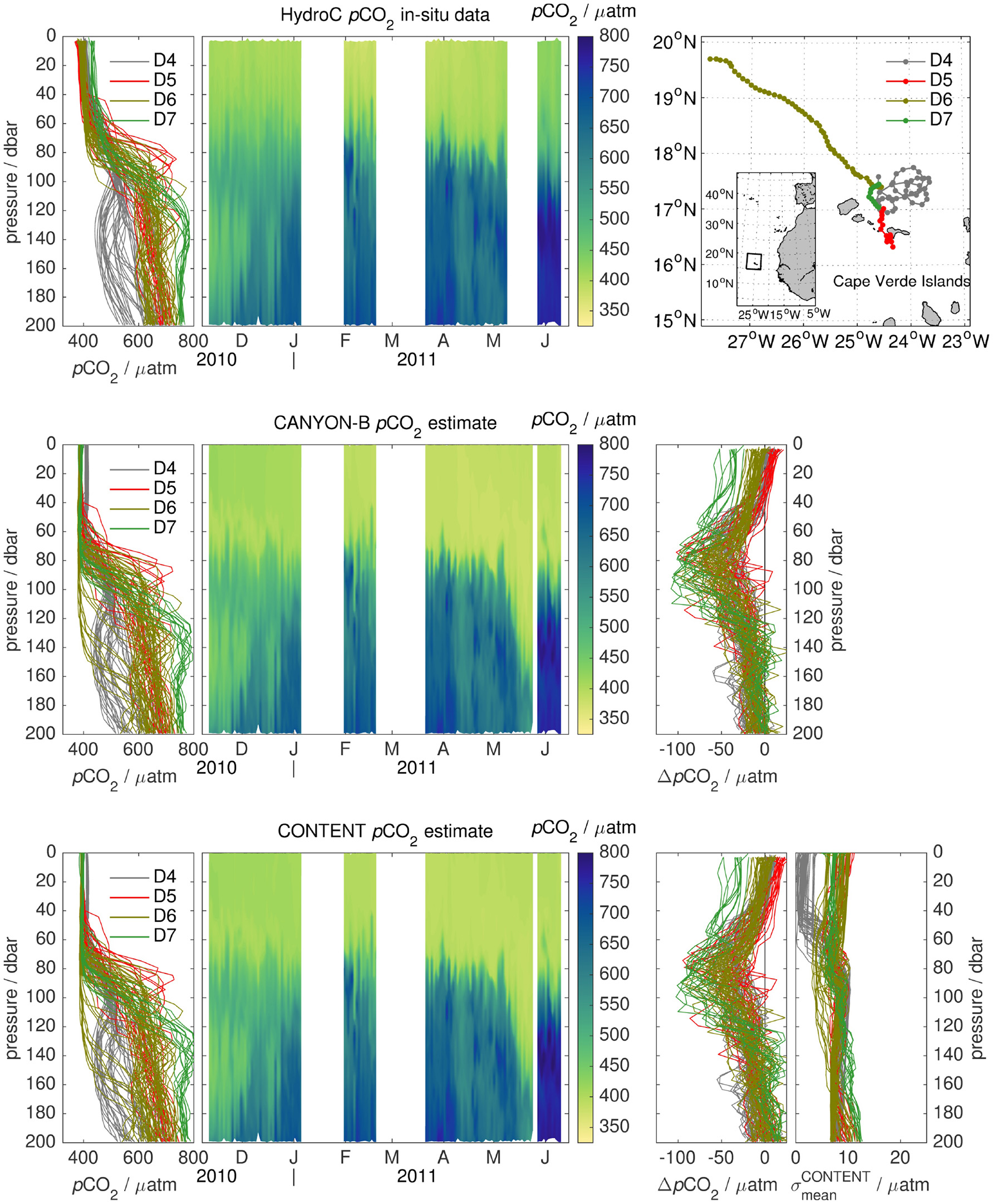
pCO2 profiles (Left), depth-time evolution (Center), and difference between pCO2 estimate and in-situ pCO2 as well as uncertainty from an incoherent carbonate system description (; right) for all four deployments D4–D7 of the experimental pCO2 float with HydroC pCO2 sensor: HydroC pCO2 sensor data (Top), CANYON-B pCO2(Middle), and CONTENT pCO2(Bottom). The profile fine structure is well reproduced and data gaps (May 2011) can be filled adequately. The mid-profile increase in ΔpCO2 is likely related to a mismatch in the time response and time lag corrections of the pCO2 (and O2) sensor in the subsurface gradients. Surface variability of CANYON-B and CONTENT pCO2 is slightly smaller than sensor data, which fits to climatological observations (not shown).
For the three deployments D4–D6 combined, CONTENT pCO2 shows negligible biases both at 200 dbar and at the surface [Table 3; bias Δ of +1 ± 12 μatm (1 std. of Δ) and +6 ± 9 μatm, respectively]. CANYON-B shows a slightly more negative difference (bias Δ of −9 ± 10 μatm and +2 ± 10 μatm, respectively), as does CANYON (bias Δ of −9 ± 16 μatm and −8 ± 13 μatm, respectively), which also has a larger spread in its biases. Biases at 200 dbar for D7 vary strongly, from a mean of +13 μatm for CONTENT to −25 μatm for CANYON. At the surface, all three methods give a pCO2 for D7 that is considerably smaller (−22 to −37 μatm) than that obtained from the float-transmitted data. Note that no post-deployment calibration was possible for D7.
Table 3
| Float deployment | D4 – D6 | D7 * | |||||
|---|---|---|---|---|---|---|---|
| Date(s) | Nov 11 – Jan 5; Jan 30 – Feb 19; Mar 20 – May 09 | May 27 – Jun 10 | |||||
| # Profiles | 44; 16; 39 | 12 | |||||
| Mean Δ ±1 std. of Δ | Mean σ | # Profiles |Δ| > σ | Mean Δ ±1 std. of Δ | Mean σ | # Profiles |Δ| > σ | ||
| Surface | CANYON | −8 ± 13 | 33 | 1/99 | −22 ± 8 | 34 | 2/12 |
| CANYON-B | +2 ± 10 | 35 | 0/99 | −37 ± 9 | 33 | 8/12 | |
| CONTENT | +6 ± 9 | 22 | 3/99 | −32 ± 9 | 22 | 10/12 | |
| 200 dbar | CANYON | −9 ± 16 | 54 | 0/99 | −25 ± 6 | 61 | 0/12 |
| CANYON-B | −9 ± 10 | 57 | 0/99 | −2 ± 5 | 68 | 0/12 | |
| CONTENT | +1 ± 12 | 34 | 0/99 | +13 ± 6 | 42 | 0/12 | |
Difference of CANYON, CANYON-B, and CONTENT pCO2 minus sensor pCO2 (in μatm) at the surface and at depth (mean Δ ± 1 std. of Δ), estimated uncertainty σ (in μatm), and number of profiles where the bias exceeds the uncertainty for the experimental pCO2 float (Fiedler et al., 2013).
The float was lost during deployment D7 (i.e., limited post-corrections).
At 200 dbar, CANYON pCO2 shows an apparent seasonal trend toward negative biases between Nov. and May, whereas no clear trend is discernable for CANYON-B or CONTENT (data not shown). At the surface, Feb./winter pCO2 seems to be slightly overestimated by CANYON-B and CONTENT, whereas D7 data in Jun. suggest a summer pCO2 underestimation.
The mean estimated pCO2 uncertainty σ of CONTENT, CANYON-B, and CANYON for D4–D6 is 34, 57, and 54 μatm at 200 dbar and 22, 35, and 33 μatm at the surface, respectively. For only three out of the 99 profiles of D4–D6, the surface bias exceeds the CONTENT uncertainty, while this is the case for none of the profiles using CANYON-B Δ and σ, and one profile using CANYON. The bias at 200 dbar does not exceed the estimated uncertainty for any of the profiles (Table 3).
The sensor data show that the CANYON-B/CONTENT mappings are able to reproduce fine structure features at the anticipated locations for pCO2. With equilibrated pCO2 sensor data, i.e., at 200 dbar and at the surface, the mean bias of CANYON-B/CONTENT pCO2 is within the sensor accuracy for profile data (Fiedler et al., 2013). The profiles tend to show a low bias (order of −50 μatm) in the lower parts of and below the mixed layer (around 80–100 dbar) (Figure 5). This is the region of strongest sub-mixed layer gradients, i.e., increasing O2 and decreasing pCO2 toward the surface mixed layer, where both the float's O2 optode and HydroC pCO2 sensor receive the strongest time lag correction. The absent or only small increase of around 80 dbar supports this notion that the low bias is caused by the CO2/O2 sensor response rather than an estimation effect (Figure 5).
As few pCO2 profile measurements exist and otherwise only pH can be measured autonomously, this comparison is very encouraging for the observation of the carbonate system depth structure. It promises to help with estimation of entrainment fluxes at the base of the mixed layer that affect the mixed layer budget of CO2 (Levy et al., 2013).
pH profiling float data and derived pCO2 profiles
Recently, the use of pH observations from Biogeochemical-Argo floats to estimate surface (and water column) pCO2 has been illustrated by Williams et al. (2017) using floats deployed in the data-sparse Southern Ocean. We want to complement their estimate with our CONTENT approach, which is shown in Figure 6 for the same four floats in the Southern Ocean that Williams et al. (2017) used.
Figure 6
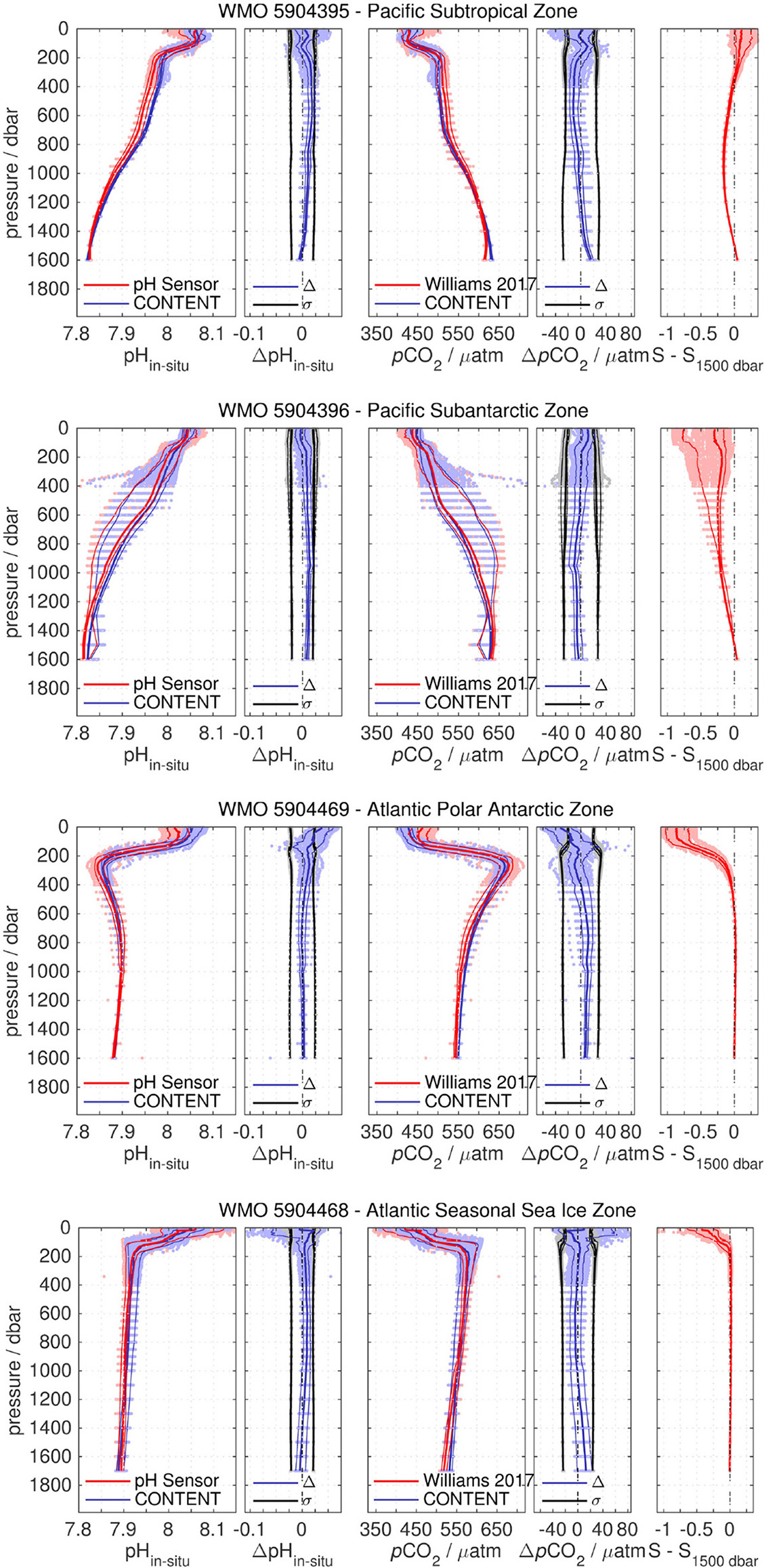
pH profile and derived pCO2 profile comparison for 4 SOCCOM Argo O2/pH floats and CONTENT. Thick and thin lines give the median and 10/90th percentiles, respectively, while pale-colored dots represent the data. From left to right: pH profile of sensor pH (red) and CONTENT pH (blue); CONTENT pH difference to sensor pH (blue) and CONTENT uncertainty estimate (black); pH-derived pCO2 profile (red) after Williams et al. (2017) and CONTENT pCO2 (blue); CONTENT pCO2 difference to derived pCO2 (blue) and CONTENT uncertainty estimate (black); Salinity profile normalized to salinity at 1,500 dbar, the depth at which the pH sensor is adjusted to an MLR-based pH. CONTENT and float-based/-derived pH and pCO2 agree within the CONTENT uncertainty but for the surface data of 5904469, where salinity is considerably different from at-depth salinity, and parts of 5904468, where biological pH increase / pCO2 drawdown is more intense than estimated by CONTENT.
For all four floats, both observed pH, which has been tuned to an MLR-based pH estimate at 1,500 dbar depth (Williams et al., 2016; Johnson et al., 2017), and CONTENT pH show the same profile shape. They agree within the CONTENT uncertainty in the entire water column below the surface mixed layer. The same is true for the comparison of pH-derived pCO2 with CONTENT pCO2.
In the upper 200 dbar and within the mixed layer, there is an increase in the difference between the floats and the neural network (compare Figure 3). For the two Pacific floats, the 10/90th-percentiles of Δ still stay within the estimated uncertainty σ. For the Atlantic float in the seasonal sea ice zone, the majority of surface data show Δ < σ, too. However, there is a considerable fraction of very high mixed layer pH /low pCO2 observed by the float in austral summer, for which the CONTENT estimates show a bias that exceeds the estimated uncertainty. Float 5904469 in the Atlantic polar antarctic zone, in contrast, is the only float that shows a systematic trend in surface pH overestimation (order +0.025) and pCO2 underestimation (order −20 μatm) by CONTENT compared to the pH sensor data. Interestingly, this coincides with a significant difference between surface salinity and salinity at 1,500 dbar (where the pH sensor data have been tuned) of almost 1 psu, which is not the case for the other floats.
Surface mixed layer performance
As shown in the previous section, surface or near-surface estimations can show an increased bias, which is why this section focusses on surface data comparisons to establish useful limits of applicability, in particular for pCO2 estimates.
Surface data are more challenging to estimate due to their higher variability and seasonality (compare the uneven seasonal coverage of the training data; Figure 1). Another challenge is surface air sea gas exchange. Oxygen is the prime predictor for ocean biogeochemistry and thus for the nutrient and C cycle. However, re-equilibration time scales for CO2 and O2 with the atmosphere are quite different, with those for O2 being an order of magnitude smaller than those for CO2 (Broecker and Peng, 1974). Surface air sea gas exchange can thus decouple C and O2 cycling in the mixed layer, as has been observed previously (e.g., Tortell et al., 2015), whereas in the interior ocean, carbon remineralization is always accompanied by a change in O2. The decoupling is particularly noticeable following intense blooms or long bloom periods (i.e., with a strong accumulated CT/pCO2 drawdown). Here, O2 is much closer to equilibrium than the CO2 system, i.e., summertime CT/pCO2 drawdown is more persistent than excess oxygen from biological production. In such cases, CANYON-B/CONTENT do not have a suitable predictor for this accumulated biological carbon imbalance (if it is not concurrent with other predictor changes, e.g., a seasonal SST change). By neglecting this accumulation effect due to the lack of a suitable predictor, CT/pCO2 will be overestimated.
Essentially, CANYON-B and CONTENT have a clear focus on water column and ocean interior variable estimation. Nonetheless, they are still useful for surface applications, keeping their limitations in mind. The comparison with in-situ data can serve to identify insufficiently represented (i.e., undersampled or uncommon) conditions. For surface applications, the mappings should be used more as an aid/tool in data analysis, not necessarily for correction of in-situ data (as is done with water column data).
Surface pCO2 derived from profiling float pH data
Figure 7 shows the surface ΔpCO2 estimated from two climatologies (Takahashi et al., 2014; Landschützer et al., 2015a), CANYON-B, CONTENT, and in-situ pH observations for the four floats. The results are mixed.
Figure 7
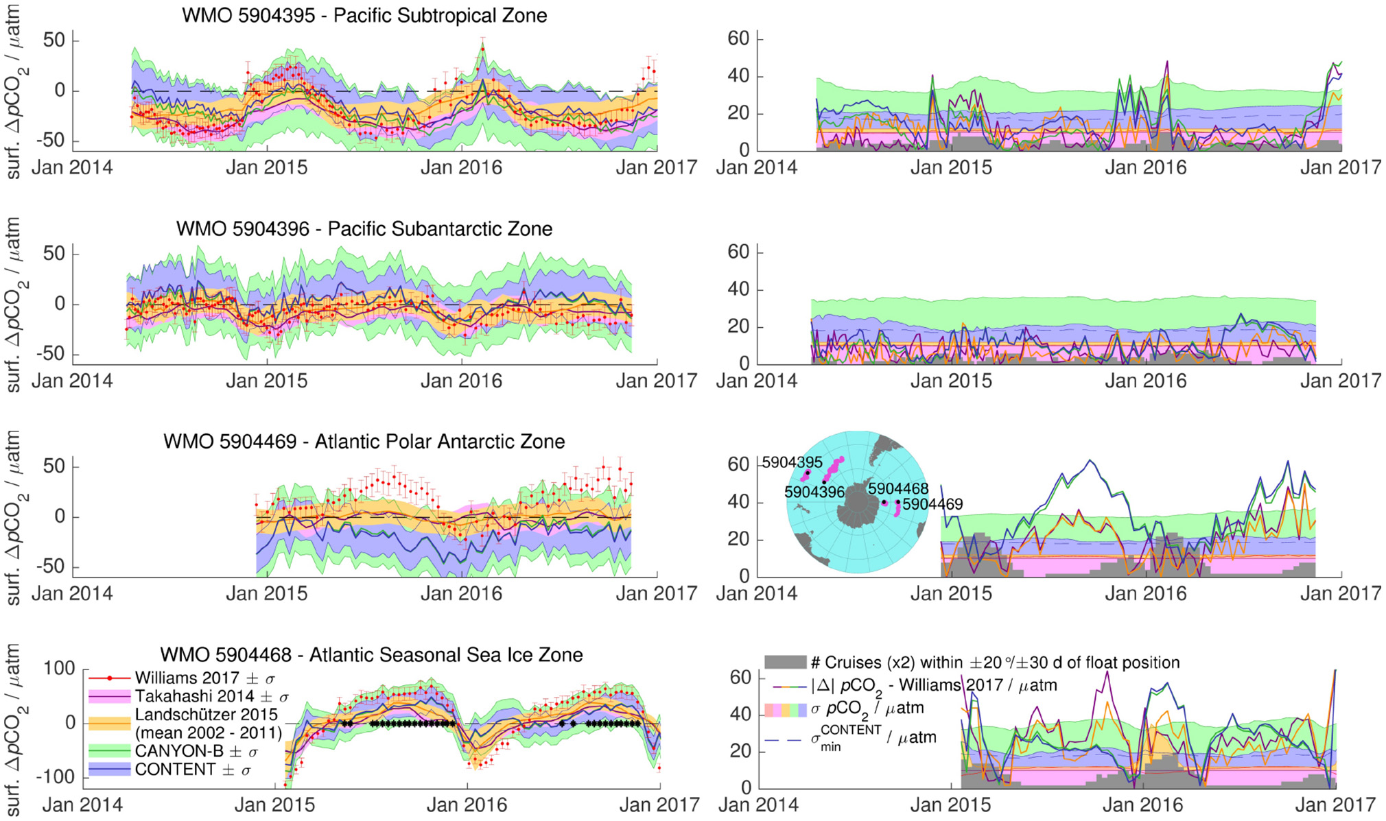
Estimates of surface pCO2 disequilibrium ΔpCO2 for four selected floats in the Southern Ocean: Takahashi et al. (2014) climatology (purple), Landschützer et al. (2015a) climatology (yellow), CANYON-B (green), CONTENT (blue), and pCO2 derived from float pH observations (Williams et al., 2017; red). The shaded areas / error bars denote the uncertainty and black asterisks under-ice profiles (only 5904468). The right panels give the absolute difference |Δ| to the Williams et al. (2017) estimate (thick lines) and the estimated uncertainty σ (shaded area) with the same color code. The gray histogram gives the seasonal coverage of cruises with carbonate system observations in GLODAPv2 and the thin dashed blue line .
For float 5904396 in the South Pacific subantarctic zone, climatological, CANYON-B/CONTENT and Williams' pCO2 show a consistent seasonal cycle. CANYON-B/CONTENT surface pCO2 is slightly higher than the other approaches, however, absolute differences to Williams pCO2 are comparable with the two climatologies and within their uncertainty bounds. In contrast, profile-to-profile variability is very similar between CANYON-B/CONTENT and Williams' pCO2. The CONTENT uncertainty shows minima close to in austral summer (Jan.), while it is elevated at the beginning of the deployment (during austral winter). The other approaches show a steady σ either by choice (CANYON-B) or by design (climatologies and Williams).
For float 5904395 in the South Pacific subtropical zone, CANYON-B/CONTENT and climatological surface pCO2 are comparable (with only some disagreements for the first couple of profiles). They match the seasonal cycle of Williams' pCO2, but show a smaller seasonal amplitude, i.e., they suggest near-neutral summer conditions instead of a small CO2 source as well as a slightly smaller winter CO2 sink than Williams' pCO2. Interestingly, CANYON-B σ is elevated during austral summer, while the CONTENT uncertainty shows little variation. Both floats in the South Pacific are in a region with very scarce training data coverage (albeit seasonally equally distributed).
A similar picture is seen for float 5904468 in the South Atlantic seasonal sea ice zone, where the temporal evolution between a summer surface CO2 sink and a winter surface CO2 source is consistent between all three estimates. However, the amplitude of the seasonal cycle for CANYON-B/CONTENT as well as for the climatologies underestimates the float-based Williams pCO2 data, so that differences to Williams' surface pCO2 mostly exceed estimated uncertainties. There is one peculiarity to note: Late austral summer (ca. Mar.) surface pCO2 for CANYON-B/CONTENT is close to atmospheric equilibrium (as is surface O2; not shown), while both climatological pCO2 as well as pH-based Williams pCO2 still show a marked pCO2 undersaturation.
Float 5904469 in the South Atlantic polar Antarctic zone shows the largest disagreements between methods. Climatological pCO2 gives near-neutral conditions year-round, while CANYON-B and CONTENT show a negative surface pCO2 disequilibrium and Williams' approach show a positive disequilibrium for most of the year. This disagreement (and in particular underestimation of surface pCO2 by CONTENT compared to Williams) has already been seen (Figure 6). Here we see that it is primarily driven by austral winter differences (where Williams' pCO2 estimates are highest), while austral summer data agree within the CONTENT (and CANYON-B) uncertainty bounds. As for float 5904468, austral summer is the period with the most training data. In contrast, the surface uncertainties don't show pronounced seasonal variability.
The two floats in the Pacific (5904395 and 5904396) operate in an area with very scarce training data (Figures 1, 7). Encouragingly, CANYON-B and CONTENT pCO2 nonetheless give comparable results to Williams' pCO2 and do not perform worse than the two climatologies, which are climatologies developed for the very purpose of estimating surface pCO2. Such climatologies use plenty of surface pCO2 data for their construction (but lack the depth dimension), whereas for the neural network mappings, surface data and dynamics are the very boundary/limit of the domain. For 5904395 in the subtropical zone, however, the seasonal cycle's amplitude is somewhat underestimated by all methods when taking Williams pCO2 as reference.
This is seen, too, for 5904468 in the (Atlantic) seasonal sea ice zone, where Williams' pCO2 shows a strong seasonal amplitude of ca. 135 μatm, while CANYON-B pCO2, CONTENT pCO2 and the two climatologies show an attenuated amplitude of ca. 75 μatm. CANYON-B/CONTENT give estimates closer to Williams' pCO2 in the early season (i.e., austral spring/early summer; Oct–Dec) while the climatologies are closer in the late season (i.e., late summer; Jan–Mar), i.e., CANYON-B/CONTENT with water mass predictors T, S, O2 give more realistic results during the melting and early bloom period, while the climatologies are better suited to capture the persistent undersaturated pCO2 levels late in the season (Figure 7), for which CANYON-B/CONTENT lacks an adequate predictor due to the different re-equilibration time scales of O2 and CO2.
Finally for float 5904469, large disagreements exist between methods, which are puzzling to us. The Williams pCO2 estimate suggests a strong CO2 source during winter, which was attributed to increased upwelling and entrainment of circumpolar deep water (with high pCO2 and CT), or an increase in pCO2 and CT of the upwelled waters (Williams et al., 2017). CANYON-B and CONTENT, in contrast, suggest an almost year-round considerable CO2 sink, while the climatologies indicate near-neutral conditions. Given that CANYON-B/CONTENT show rather good performance on interior ocean data (e.g., Figures 3, 4), we would expect an interior ocean signature (from upwelling/entrainment) to be appropriately propagated to surface waters and thus be somewhat reflected in the surface predictions.
What's different to the other floats is the strong salinity difference between depth and surface. Salinity plays a role for the potential difference between the ISFET pH probe and the silver chloride reference electrode of the sensor, and is taken into account in the calculation of pH (Johnson et al., 2016). Moreover, sensor diagnostics don't indicate any malfunction of the probe (T. Maurer, J. Plant, K. Johnson, pers. comm.). Still, the concurrence with the salinity depth-surface difference lets us speculate whether the pH (and thus Williams' pCO2) differences might be due to a dynamic effect (i.e., “salinity time response”)? On the other hand, CANYON-B/CONTENT depend on the salinity input, too, i.e., the strong mismatch could be caused by a systematic issue on surface CANYON-B/CONTENT pH or pCO2, for which we do not have an indication either.
As surface pCO2 estimates agree within their uncertainty during austral summer (Jan.–Mar.) when training data and other surface pCO2 observations are available for the area, while disagreements peak during winter in the absence of training/reference data, we may suspect both climatological as well as CANYON-B/CONTENT surface predictions during winter. Arguably, one would expect Williams' pCO2, based on (presumably accurate) pH observations together with a locally tuned MLR for AT, to give the “best” result. At the same time this illustrates a limit of the CONTENT coherence portion: While for this float the CANYON-B CO2 variables are very coherent throughout the deployment (i.e., σCONTENT is close to ; Figure 7), they still could be wrong. In other words, the absence of elevated σCONTENT does not guarantee that predictions are accurate. The uncertainty estimate needs always to be combined with a second quality indicator, the training data coverage.
These examples show that there is still considerable uncertainty associated with estimating surface ΔpCO2 in the Southern Ocean, and consequently the direction and magnitude of its CO2 source/sink status (e.g., Landschützer et al., 2015b). In particular for frontal areas (e.g., Polar Antarctic Zone) or rarely observed areas/conditions (e.g., austral winter), disagreements between the methods can be significant. At the same time, profile-to-profile (i.e., short-term) variability between CONTENT pCO2 and Williams pCO2 are extremely consistent, which may offer new ways to address spatial/temporal variability.
Direct surface pCO2 underway observations
The comparison between surface pCO2 underway data across the Atlantic and neural network-derived pCO2 from CANYON, CANYON-B, and CONTENT is given in Figure 8 along with their quality indicators (uncertainty σ and training data coverage).
Figure 8
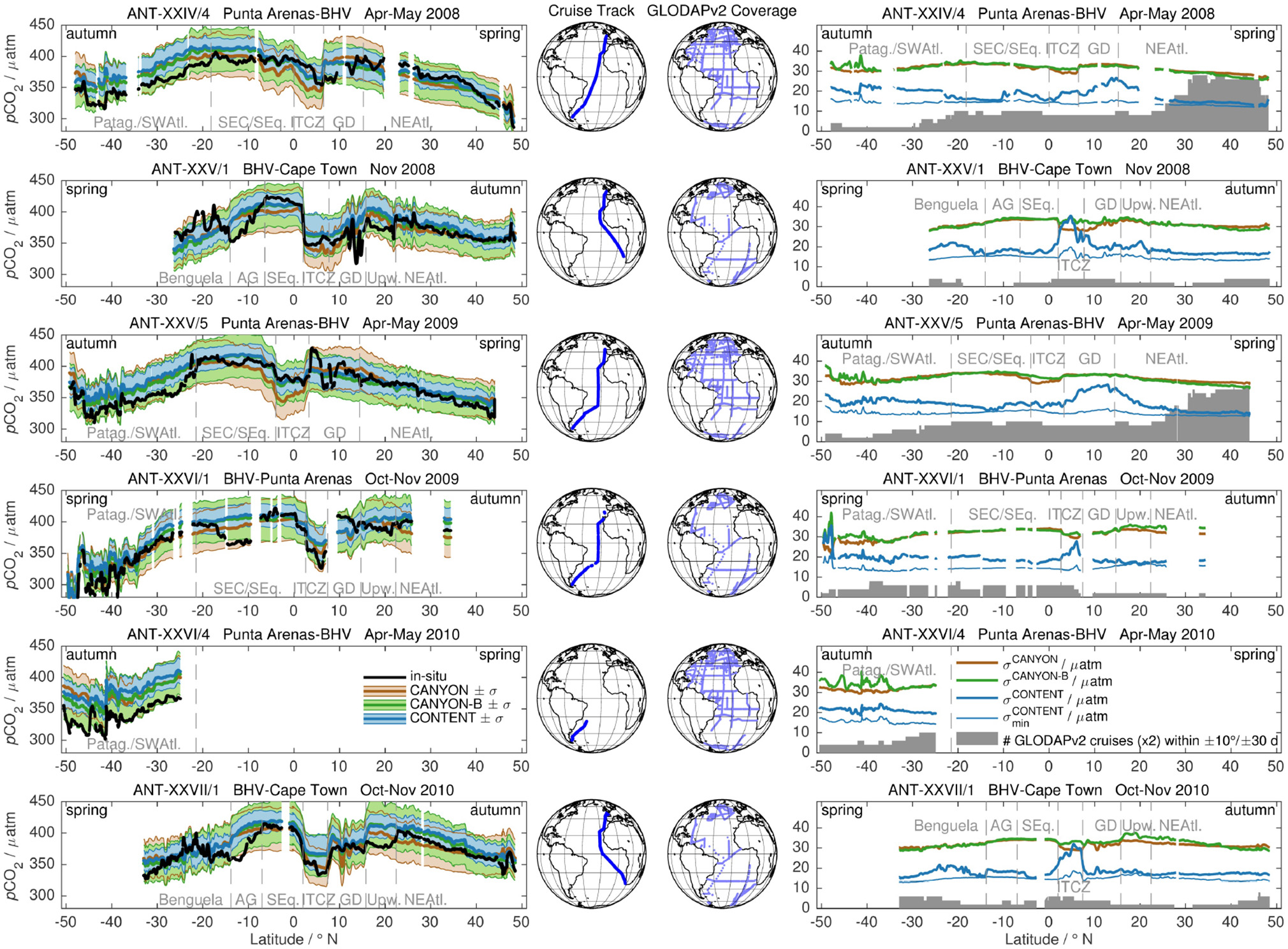
Surface underway pCO2 data during six R/V Polarstern transects across the Atlantic Ocean, three northbound austral autumn/boreal spring cruises (panels 1, 3, and 5, top to bottom) and three southbound austral spring/boreal autumn cruises (panels 2, 4, and 6). (Left) For each cruise, CANYON pCO2 (brown), CANYON-B pCO2 (green), and CONTENT pCO2 (blue) are shown with their respective uncertainty interval (shaded). In-situ observations are given in black. Regions are denoted by gray dashed lines: Patagonian Shelf and South West subtropical Atlantic (Patag./SWAtl.), South Equatorial Current (SEC) and South Equatorial (SEq.) region, Benguela Current region, Angola gyre (AG), Inter Tropical Convergence Zone (ITCZ), Eastern tropical North Atlantic and Guinea dome (GD), Mauritanian upwelling region (Upw.), and Eastern North Atlantic (NEAtl.). (Middle) Maps show the cruise tracks as well as the GLODAPv2 surface carbonate system data coverage of the neural network training data around the cruise dates (April/May and mid-October to mid-December, respectively). (Right) For each cruise, the gray histogram gives the training data coverage as number of cruises within a box of ±10° and ±30 d (yearday) around the observation. Thick colored lines give the methods' uncertainty estimates (brown, green, and blue, respectively), while is given as thin blue line.
The three estimates give a similar result for surface pCO2 and agree with observed large-scale trends, e.g., an increase in surface pCO2 in tropical areas compared to subtropical/subpolar ones, or a depression in sea surface pCO2 in the Inter Tropical Convergence Zone (ITCZ) as well as its seasonal migration (around 6° N for Oct./Nov. cruises and around 1° N for Apr./May cruises; see also Tomczak and Godfrey, 1994). CANYON-B and CONTENT tend to somewhat outperform CANYON in tropical regions, while CANYON shows a slightly smaller bias than CANYON-B or CONTENT in the Eastern subtropical North Atlantic. All three methods show comparable results in the South Atlantic both in the Angola gyre (AG) and Benguela current area for cruises to Cape Town (ANT-XXV/1, ANT-XXVII/1) as well as off the Patagonian shelf (Patag./SWAtl.) for cruises from/to Punta Arenas.
There is a general tendency for the neural network-based methods to overestimate surface pCO2. This is clearly seen off the Patagonian shelf, where austral autumn (Apr.) pCO2 is consistently overestimated (+20 μatm) while austral spring (Nov.) estimates fit well to in-situ pCO2 levels. Similarly, some cruises (ANT-XXIV/4 and in particular ANT-XXVI/1, ANT-XXV/5 possibly, too) show pronounced low in-situ pCO2 on a spatial scale of few degrees that is not mirrored by the neural network methods. Similar low in-situ pCO2 patterns have been observed for three other SOCAT cruises (cruises 29HE20051019, 740H20121011, and 74JC20131009). Finally, low in-situ pCO2 is overestimated by up to +30 μatm in the upwelling area (Upw.) off the Mauritanian coast in the North Atlantic for Oct./ Nov. cruises. The coastal upwelling is a seasonal phenomenon that has its maximum close to the coast in spring (Mittelstaedt, 1983). The lower-than-estimated pCO2 signature is more pronounced in the 2008 and 2010 cruises (ANT-XXV/1, ANT-XXVII/1) closer to the coast than in the 2009 cruise (ANT-XXVI/1), which passed ca. 200 nm farther offshore. In contrast, Apr./May pCO2 seems to be consistently underestimated (−20 μatm) in the Western ITCZ/equatorial region by CANYON, while CANYON-B/CONTENT estimates agree better with in-situ data.
Furthermore, the region of the Guinea dome (GD) shows a high variability in in-situ pCO2, which is not always captured by the neural network estimates (e.g., ANT-XXV/1, ANT-XXV/5). Its estimates can be biased high (e.g., ANT-XXIV/4) or low (e.g., ANT-XXVI/1). Similarly, in-situ data diverges from estimates across the Angola gyre (AG) as well as the Benguela current system and the upwelling area off Namibia with a consistent pattern for both cruises. These areas and season are least-covered by the GLODAPv2 training data.
The CANYON and CANYON-B uncertainty are of similar magnitude. While CANYON's σ simply follows the estimated pCO2 (e.g., a decrease in σ in the ITCZ where pCO2 is lower), CANYON-B shows some elevated levels along the Patagonian shelf, where in-situ pCO2 variability is high. CONTENT's σ, in contrast, is of considerably smaller magnitude, with pronouncedly elevated levels (above ) for boreal spring (May) cruises across the Guinea Dome, within the ITCZ, and to some extent along the Patagonian shelf/South West Atlantic. However, in areas of surface pCO2 overestimation and high surface pCO2 variability like along the Patagonian shelf, CONTENT tends to give estimates with |Δ| > σ when compared to in situ data.
The tendency of neural network overestimation of pCO2 is also visible in the bulk statistics/metrics for all six cruises combined (Table 4). The median CANYON-B and CONTENT biases are +7 and +10 μatm, respectively, while CANYON appears to have the smallest bias with a median of +3 μatm. However, for all three methods the 10/90th-percentiles indicate a clear asymmetry toward overestimation. The median uncertainties of CANYON and CANYON-B are comparable (31 and 32 μatm), while CONTENT states a considerable smaller σ (18 μatm). With respect to co-location of Δ and σ, there is a comparable picture for data underestimation, i.e., Δ < –σ, for CANYON (2.5%), CANYON-B (2.0%), and CONTENT (3.6%), despite the much smaller σCONTENT. CANYON and CANYON-B have a similar fraction of data overestimation, i.e., Δ > +σ (5.5 and 4.1%, respectively). For CONTENT, as already seen above, this fraction is significantly higher (30.9%). In total, CANYON-B has a smaller fraction of |Δ| > σ (6.0%) than CANYON (8.0%), while about one third (34.5%) of CONTENT biases are outside the stated uncertainty, mostly due to overestimation.
Table 4
|
surface pCO2
Δ / μatm |
surface pCO2
σ / μatm |
|Δ| > σ / % | |
|---|---|---|---|
| 10 / 50 / 90th | 10 / 50 / 90th | – / + / ∑ | |
| CANYON | −18 / +3 / +27 | 29 / 31 / 34 | 2.5 / 5.5 / 8.0 |
| CANYON-B | −12 / +7 / +27 | 29 / 32 / 34 | 2.0 / 4.1 / 6.0 |
| CONTENT | −9 / +10 / +32 | 16 / 18 / 22 | 3.6 / 30.9 / 34.5 |
| Landschützer et al. (2017) | −15 / +2 / +18 | 12 / 12 / 12 | 13.8 / 22.4 / 36.2 |
Comparison between neural network (CANYON, CANYON-B, and CONTENT) surface pCO2 and in-situ underway pCO2 data, as well as between a smoothed monthly climatology (Landschützer et al., 2016, 2017; based on SOCAT data, which includes our underway data) and in-situ underway pCO2 data: Bias Δ (in μatm) with 10/50/90th percentile, estimated uncertainty σ (in μatm) with 10/50/90th percentile, and fraction of data (in %) where bias exceeds uncertainty (– / + / ∑ denotes underestimation, overestimation, and total, respectively).
Note that CANYON suffers from the same systematic overestimation issues in productive regions as CANYON-B/CONTENT (see discussion). For CANYON, those are accompanied by underestimation in other areas (e.g., in the tropics; Figure 8), which gives a small median bias but not thanks to better performance.
For comparison, a smoothed monthly climatology (Landschützer et al., 2016, 2017; not shown in Figure 8) gives a small median bias of +2 μatm and a similar width of biases Δ for underestimation as the neural network approaches (distance 10th percentile-median of about 18 μatm). The tail of the Δ distribution for overestimation is slightly smaller for the climatology compared to CANYON/CANYON-B/CONTENT (distance median-90th percentile ca. 16 μatm vs. 20–24 μatm, respectively). With a stated uncertainty of 12 μatm (Landschützer et al., 2014), a total of 36.2% of the data differences Δ exceed σ, with some tendency for preferential Δ overestimation, but not as pronounced as for CONTENT. Note that this is not a completely independent comparison, as the six R/V Polarstern cruises are part of SOCAT, on which the climatology is based.
The Patagonian shelf, as well its slope area, is well known for intense spring and summer blooms with a tight coupling between surface chlorophyll a and ΔpCO2. Autumn ΔpCO2 air sea disequilibria between −30 and −40 μatm are typical (Bianchi et al., 2009). The consistent austral autumn (Apr.) overestimation of pCO2 along the Patagonian shelf is a clear example of surface O2 being an imperfect predictor for surface pCO2. Moreover, autumnal training data coverage is scarce and σCONTENT levels are elevated (Figure 8). CANYON-B/CONTENT are thus hard-pressed to provide reliable predictions, which is expressed in both quality indicators.
The same effect can be seen in the North Atlantic off the Mauritanian coast for the Oct./ Nov. cruises. Coastal upwelling (Upw.) fuels biological production that causes a reduction in surface pCO2, which is advected offshore (Jones and Folkard, 1970; Huntsman and Barber, 1977; Mittelstaedt, 1991; Messi and Chavez, 2015). The strength of this seasonal phenomenon does not seem to be captured by the CANYON/CANYON-B training either, yielding offsets of up to +20 μatm for the estimates (and being more intense for the near-coastal than for the off-shore cruises).
Similarly, the drop in observed pCO2 in the SEC region is potentially a signature of past productivity associated with the seasonal Atlantic Cold Tongue (ACT) in the Eastern tropical Atlantic (e.g., Schott, 1942) that was advected into this area. The ACT correlates with the entrainment of nutrient-rich waters that fuel surface production (Grodsky et al., 2008) and consequently reduces in-situ pCO2.
These examples show how divergence between neural network estimates and in-situ data can help to identify special ocean conditions (past upwelling or advected past productivity, in our cases). In fact, they illustrate an alternative value of CANYON-B/CONTENT for surface pCO2 applications: While appearing incoherent at a first look, many of the differences between observed surface pCO2 and CONTENT pCO2 have biogeochemical reason, i.e., instead of substituting for an actual surface pCO2 observation (about one third of the surface pCO2 are overestimated by CONTENT, Table 4), CONTENT surface pCO2 should be used for quality control/validation as well as interpretation through identification of “uncommon” features or “past productivity” conditions.
For such an application, CONTENT pCO2 seems to be more suited than CANYON-B (or CANYON) pCO2. First, CONTENT's uncertainty σ is considerably smaller and second, CONTENT has the tendency to give slightly higher pCO2 than CANYON-B (by a few μatm), both of which make it more sensitive to lower-than-expected (i.e., climatological) pCO2. When neglecting the accumulated low pCO2 areas outlined above, the CONTENT bias exceeds its (small) uncertainty estimates only in areas of high variability and low training data coverage (e.g., Benguela current/Angola gyre area or the Guinea dome; Figure 8). This increase can be attributed to the limitations of the underlying training data not fully reflecting the dynamics of these highly variable ocean areas (e.g., the Guinea dome, Oettli et al., 2016).
Moreover, the underway data illustrate that focussing on one bulk metric alone (e.g., the bias Δ) can be misleading: From Table 4, CANYON appears to have the lowest (median) bias. However, it possesses the same systematic overestimation problems for accumulated biological pCO2 drawdown (i.e., the lack of a suitable predictor) as CANYON-B and CONTENT. These overestimations are complemented by underestimations in other areas (e.g., the tropics), causing an apparently smaller median bias than for CANYON-B/CONTENT, which, in fact, both show a better performance in the tropics. Focusing on the bias only would thus give a false impression, which is why we use all three metrics together for our assessment.
Global surface pCO2 from water column data and CANYON-B/CONTENT
One advantage of the CANYON-B/CONTENT mappings (based on the GLODAPv2 collection of hydrographical data) is its transferability to a different observation network (e.g., Argo-O2). This way, one can take advantage of the unbiased temporal sampling of Argo floats (Figure 1) to complement another observation network, i.e., surface underway pCO2 lines.
From the transfer data set of WOD-O2, GLODAPv2-O2, and Argo-O2 profiles, we used the shallowest profile observation together with CANYON-B and CONTENT, respectively, to estimate a climatological, global surface pCO2. CANYON-B/CONTENT pCO2 was compared to a smoothed monthly surface pCO2 climatology for the period 1982–2015 (Landschützer et al., 2016, 2017), which is based on SOCAT itself (Figure 9 for CONTENT results). For reference, the SOCATv5 monthly gridded surface pCO2 (Bakker et al., 2016) was compared to the same climatology for better assessment.
Figure 9
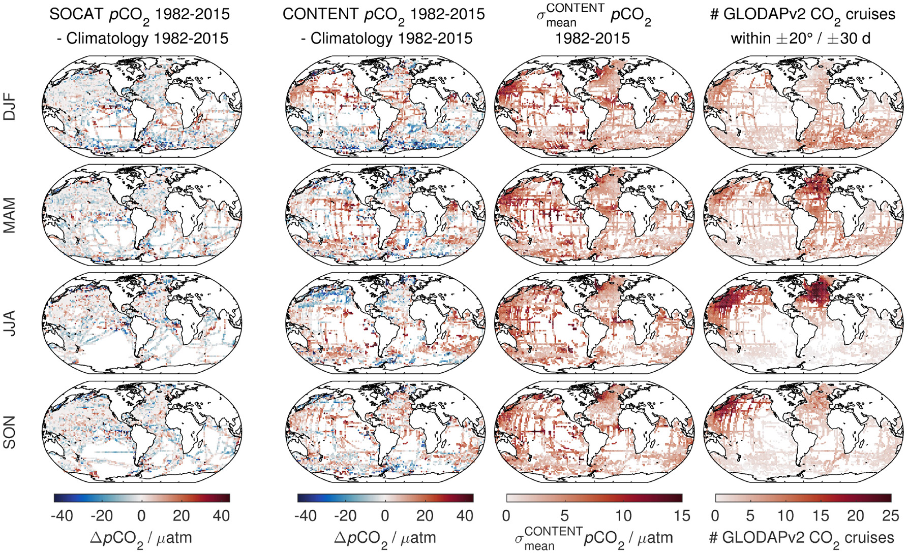
Comparison of the SOCATv5 data and CONTENT pCO2 estimates for the transfer data set to the Landschützer et al. monthly surface pCO2 climatology for the period covered by the climatology (1982–2015) and the months of December/January/February, March/April/May, June/July/August, and September/October/November (top to bottom), respectively. From left to right, the first panel shows the difference between SOCAT data and the climatology, the second panel the difference between CONTENT and the climatology, the third panel the CONTENT uncertainty contribution from an inconsistent CANYON-B carbonate system, and the last column the number of GLODAPv2 cruises with carbonate system data within ±20° and ±30 days (doy). Estimates in the tropical / subtropical Northeast Pacific seem to be systematically biased high (2nd from left), potentially related to low training data coverage (right panels). Both SOCATv5 and CONTENT give lower pCO2 than the climatology in the high latitude Southern Ocean during austral summer (DJF). In contrast, while CONTENT pCO2 is low in the high latitude North Pacific during boreal summer (JJA), SOCAT, and climatology pCO2 agree.
The comparison gives a mean difference to climatological surface pCO2 of −1 ± 13 μatm for SOCATv5 surface data, of −1 ± 16 μatm for CANYON-B with the transfer data set, and +2 ± 17 μatm for CONTENT with the transfer data set, i.e., the estimates are not significantly biased. The fraction of |Δ| exceeding the combined uncertainty σ of the climatology (12 μatm, Landschützer et al., 2014) and of the method (5 μatm for SOCATv5 data, σCANYON−B, and σCONTENT) is 18.3, 4.2, and 12.1% (approx. equal portions of over- and underestimation), with a mean combined uncertainty of 13, 33, and 23 μatm for SOCATv5, CANYON-B, and CONTENT, respectively.
The comparison between SOCATv5 and the Landschützer et al. climatology basically gives information about the mapping error when creating the smoothed, monthly climatology, as well as the noise of the SOCAT source data (Figure 9, left). Unsurprisingly, there is no mean bias between the two and the bias' standard deviation matches the method's stated uncertainty (Landschützer et al., 2014).
What's important to note is that the source data of SOCATv5 and our CANYON-B/CONTENT estimate are different, i.e., the CANYON-B-/CONTENT-based transfer data set estimates are truly independent from the climatology and SOCAT. With this in mind, the comparison is very encouraging with an unbiased mean difference and a spread in the bias that is only 25% higher than for the SOCAT source data. Nonetheless it appears that the biases occur less randomly than for SOCAT, i.e., they appear to cluster regionally (e.g., underestimation of pCO2 in Dec/Jan/Feb close to the Antarctic continent; overestimation in the Northeast and subtropical Pacific compared to the climatology). What's encouraging is that some of these patterns can be seen in the SOCAT—climatology comparison, too (e.g., Dec/Jan/Feb high latitude Southern Ocean underestimation), or that they are accompanied by an elevated (e.g., Northeast and subtropical Pacific).
Surface pCO2 observations in SOCAT are Northern hemisphere-focused and summer-biased in high latitudes. Conversely, floats provide the same data density winter and summer (Figure 1). Moreover, WOCE/CLIVAR/GO-SHIP repeat hydrography observations as well as Biogeochemical-Argo observations of O2 cover areas that are not frequented by commercial shipping. They can thus extend observations and provide proxies for seasonal variability, even if their CANYON-B/CONTENT pCO2 estimate itself may be of lower accuracy than direct observations, and thus help to fill spatial gaps in SOCAT data (e.g., in particular in the Southern hemisphere; Figure 9). The CANYON-B/CONTENT surface pCO2 estimation presented here thus represents an actual extension of the surface pCO2 database. This is relevant for global CO2 flux estimation efforts such as the Surface Ocean CO2 Mapping intercomparison (SOCOM; Rödenbeck et al., 2015). However, only variability observed by WOCE/CLIVAR/GO-SHIP can be reproduced by CANYON-B/CONTENT at present. With large gaps in surface pCO2 observations in the Southern Ocean and during winter, the prospect to fill these gaps through mapping methods such as CONTENT pCO2 is promising, but is still associated with quite large uncertainties. Still, some major driving factors of carbonate chemistry are captured by CONTENT even within such “gaps,” which is visible in the short-term variability. When assessing the quality of CONTENT estimates, both σCONTENT and the training data coverage should therefore be included in the assessment.
Apart from the spatio-temporal aspect, CANYON-B/CONTENT pCO2 is based on water column data, i.e., it provides the depth of the mixed layer that is relevant for gas exchange in parallel to an estimate of the pCO2 profile, a dimension that is critically lacking from surface underway observations. This will help improve CO2 flux and budget estimates even in regions in which the surface disequilibrium is well characterized by other means. In fact, the promising applications will therefore come from the linking of observation systems (e.g., Biogeochemical-Argo and voluntary observing ship lines) and data sets (e.g., CONTENT pCO2 for the water column structure and SOCAT for accurate surface pCO2, respectively).
Complete carbonate system description: analysis of the revelle buffer factor
CONTENT provides an estimate of the complete state of the carbonate system. Below, we use this technique to get a better view of the global distribution of the Revelle buffer factor. Sabine et al. (2004) report R values in the range from 9 to 15 for the year 1994, which is already about 1 unit higher than in the pre-industrial ocean due to the uptake of anthropogenic CO2 (Sabine et al., 2004).
With the transfer data set, we obtain a similar mean distribution of R as presented by Sabine et al. (2004) (Figure 10, left; mean year 2005). Further analysis of these observation-based estimates reveals a decadal trend in R with a global mean of +0.18 ± 0.14 (1 std.) units per decade (Figure 10, middle and right). In some regions, the increase in R is stronger than the global mean, in particular in cold surface waters (e.g., subpolar North Atlantic/Pacific and Southern Ocean). There, we observe an average trend of +0.25 ± 0.16 (1 std.) units per decade (North of 45° N) and of +0.30 ± 0.12 (1 std.) units per decade (Southern Ocean; South of 45° S), respectively, which is about 50% larger than the global average and more than twice as large as the trend at lower latitudes below 45° N/S (+0.12 ± 0.09 units per decade).
Figure 10
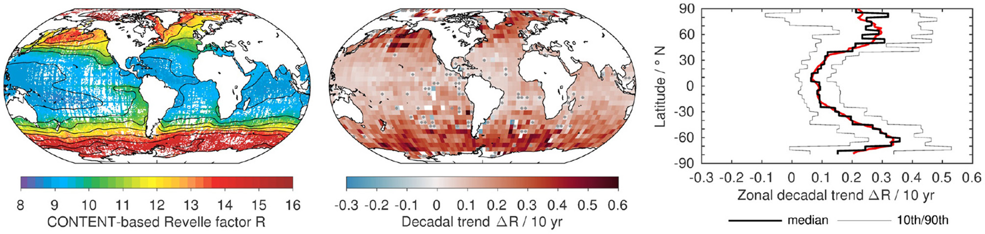
Revelle factor R calculated with CONTENT CT and AT for the transfer data set (Left) and derived decadal trend in R(Middle and Right). The global pattern of R matches the picture of Sabine et al. (2004). Linear trends were derived per 5° x 5° grid box that has data of at least 3 individual years spanning at least 10 years (insignificant trends are denoted by gray dots). The zonal median trend (thick line) and its 10/90th percentiles (thin lines) are shown in black, while the red line gives the smoothed zonal median trend (Right).
Along the same lines, the analysis of the Revelle factor R shows the value of CANYON-B/CONTENT on a climatological scale. In fact, we believe this is the first global observation of the increase in R apart from sensitivity considerations (e.g., Fassbender et al., 2017) or model studies (e.g., Thomas et al., 2007; Hauck and Völker, 2015). The magnitude of the increase fits perfectly with what has been observed at selected CO2 time series sites (range +0.11 to +0.30 units per decade; Bates et al., 2014) as well as with surface pCO2 climatology-based estimates (range +0.1 to +0.4 units per decade, Fassbender et al., 2017). Similarly, the higher trend in R in cold surface waters has been suggested from sensitivity considerations (e.g., Thomas et al., 2007; Fassbender et al., 2017). Such an elevated trend at higher latitudes is particularly important for the current and future uptake and sequestration of anthropogenic CO2 through the solubility pump, as deep and intermediate water masses are formed in these areas. It should be noted, however, that our estimates at very high latitudes (Arctic ocean and near the Antarctic continent) are nonetheless based on few observations and show the highest variability. The significance of the slight decrease in the trend in R toward the poles estimated by this study might thus be debatable.
This illustrates the capacity that knowledge or improved estimates of the oceanic carbonate system gives to ocean biogeochemistry and global climate science.
Discussion
Comparison between a static climatology, CANYON, CANYON-B, CONTENT, and LIR
Figure 11 shows the distribution of AT at 400 m depth as an example for the prediction by a classical (“static”) climatology (GLODAPv2 mapped climatology, Lauvset et al., 2016), neural network approaches like CANYON and CANYON-B, CONTENT, and a regression approach such as LIR. All methods but the first use climatological fields of T, S, and O2 as input data.
Figure 11
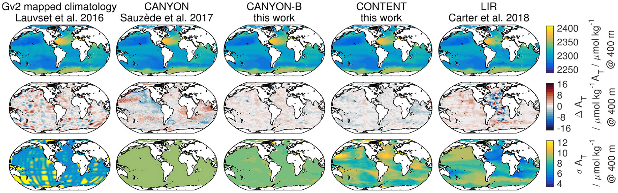
Example of estimated AT distribution at 400 m using different (climatological) mapping methods: GLODAPv2 mapped climatology (Gv2), CANYON, CANYON-B, CONTENT, and LIR. All but the mapped climatology use climatological fields of T, S, and O2 at 400 m as inputs. Panels from top to bottom give the distribution of AT, the difference between the individual method's AT and the median AT of Gv2, CANYON, CONTENT and LIR, and estimated AT uncertainty.
The distribution of AT between all five methods is comparable, with a similar overall range as well as a similar spatial distribution. The estimated uncertainty σ, however, shows a markedly different character: For the mapped climatology (Gv2), minima are observed along repeat hydrography lines (compare Figure 1) while mapping errors increase strongly in between lines. CANYON's constant uncertainty σ ignores both the underlying training data distribution (along repeat hydrography lines) as well as oceanic structures. CANYON-B's σ shows some local structure, e.g., with slightly elevated levels along the Antarctic circumpolar current (ACC), in Eastern boundary upwelling areas, or in the subtropical Pacific at the edges of the oxygen minimum zone. However, CONTENT's and LIR's σ are much more variable and nuanced, i.e., they cover a wider range of uncertainties and oceanographic features or structures are clearly visible, e.g., the Kuroshio extension, in which CONTENT shows elevated while LIR shows reduced σ AT, the ACC region, or fronts and gyre boundaries.
For better comparison, the anomalies Δ of predicted AT to the median value of Gv2, CANYON, CONTENT, and LIR as the best guess of “true” AT are also shown in Figure 11. (CANYON-B was not included in the median as its result is already inherent to our implementation of CONTENT.) As for the uncertainty, the Gv2 anomaly Δ shows a grid-like structure. CANYON, CANYON-B, and CONTENT Δ's follow oceanic features or water masses, where CANYON's anomalies are of significantly higher magnitude than those of CANYON-B or CONTENT. LIR shows similar (low) Δ in the Pacific, but elevated differences (with alternating sign) in the Atlantic basin for this example.
Mapping character and predictor limitations
A classical climatology provides a mapping between a variable and the spatial coordinates (or predictors) latitude, longitude, and depth. A regional MLR provides a mapping between a variable of interest (e.g., AT) and other variables (e.g., T, S, O2) as predictors. Our neural network approaches mix these two end-members to provide a mapping that depends on other observed variables, but in a spatially varying way (for global coverage). In comparison with a classical climatology with predictors lat, lon, and P, mapping techniques like CANYON-B, CONTENT, LIR, etc. simply use a wider range of predictors (lat, lon, P, T, S, O2), which allows them to react more flexibly, e.g., to a different water mass characteristic. In the end, they are based on the available observations, which is why we denote their mappings as “dynamic climatology.”
This difference is nicely illustrated by Figure 11. The GLODAPv2 mapped climatology (Lauvset et al., 2016) has largest mapping errors in between repeat hydrography lines due to the strictly spatial mapping. The uncertainty of CANYON-B/CONTENT/LIR, in contrast, is elevated along oceanographic features such as fronts, gyre boundaries, upwelling areas, etc., illustrating the “dynamic” character of these mappings. Here, CONTENT and LIR show the widest distribution of σ, i.e., the largest adaptation of σ to the local conditions (Figures 3, 4, 11). CANYON, in contrast, is ignorant to where predictions are made—variations in σ only originate from the measurement uncertainty, σmeas.
The “dynamic” climatologies, however, can only adapt to local conditions for which they have adequate predictors. If there is no suitable predictor available for a given process (e.g., denitrification; or accumulated surface pCO2 disequilibrium), there is little potential to reproduce observations impacted by such processes except for in a climatological (i.e., mean state-) sense. Elsewise, they can be employed as simple-to-use transfer functions to assess what a variable of interest would look like (again, in a climatological sense) with the given predictor inputs, much like a “classical” climatology.
Thus they represent an alternative interesting way to densify “virtual” observations of some costly acquirable variables from the sole knowledge of simply and cost-effectively acquirable variables. In such sense these dynamic climatologies have a great potential to take benefit from emerging networks of autonomous platforms (e.g., BGC-Argo) for filling observational gaps of some key variables.
Scale analysis
The notion of good representation of profile-to-profile surface variability between Williams pCO2 and CANYON-B/CONTENT pCO2 can be supported by an analysis of the power spectrum of the respective time series (Lomb, 1976; Scargle, 1982) (Figure 12). In effect, the Williams pCO2 series shows a higher spectral power than the climatologies (Takahashi et al., 2014; Landschützer et al., 2015a) at all time scales from 20 to 365 days. CANYON-B and CONTENT pCO2 show a somewhat lower power than Williams pCO2 at long time scales (comparable to the climatologies), however, for scales shorter than ca. 100–120 days, they approach or match the spectral power of the float data. In addition, the spectral power of the difference between climatology/CANYON-B/CONTENT and Williams is markedly attenuated for CANYON-B/CONTENT compared to the climatologies for time scales between 40 and 120 days.
Figure 12
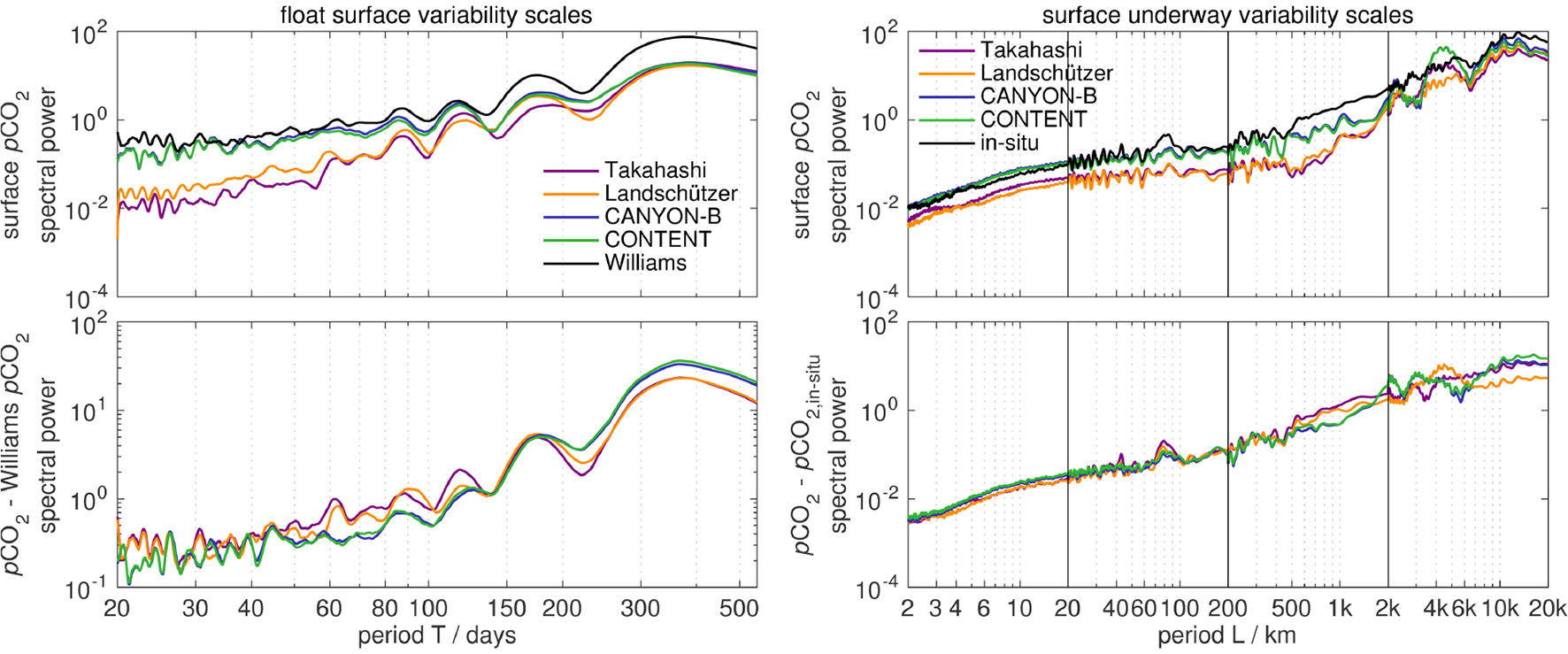
Power spectra of temporal (Left) and spatial (Right) variability of surface pCO2(Top) and difference between estimated pCO2 and float-derived/in situ pCO2(Bottom). The “dynamic climatologies” (CANYON-B, CONTENT) resemble the observations more closely than classical climatologies (Takahashi, Landschützer) at smaller scales (<120 d, <1,500 km).
A similar analysis can be done for the surface underway pCO2 data (Figure 12) with a quasi-synoptic assumption, i.e., for each cruise the variability is assumed to be only spatial, not temporal. Again, the in-situ data shows a higher spectral power than the climatologies at all scales (2 to 20,000 km). The power spectrum of CANYON-B/CONTENT is comparable to the climatologies at long scales (>6,000 km), while it approaches the intensity of the in-situ data at scales of 500–1,500 km, and shows a similar power as in-situ data for smaller scales (<500 km). The power spectrum for the difference between climatology/CANYON-B/CONTENT and in-situ pCO2 shows the largest difference at scales of 500–1,500 km, where CANYON-B/CONTENT show a lower power than the climatologies. At large scales (>6,000 km), the difference of climatology—in-situ shows a somewhat smaller spectral power than their CANYON-B/CONTENT counterparts.
The scale analysis of surface pCO2 provides two conclusions: (1) The spectral behavior at smaller scales (mesoscale, monthly/sub-seasonal) is comparable between the CANYON-B/CONTENT mappings and in-situ observations. In particular the larger portion of this range (i.e., 500–1,500 km; 40–120 days) shows an improved coherence. This reflects the influence of the “dynamic” predictors T, S, and O2, which implicitly cover certain surface driving mechanisms. (2) The spectral behavior at large scales is comparable between the CANYON-B/CONTENT mappings and a classical climatology. This reflects the climatological character of both approaches, which are based on the same “climatological scale” (i.e., basin-wide, multi-year) GLODAPv2 data set.
Thus, despite some identified systematic shortcomings under certain conditions (see above), dynamic climatologies such as CANYON-B or CONTENT offer new ways to approach small-scale variability that are unaddressed with classical climatologies. Moreover, they are useful transfer functions to connect different parts of the ocean observation system but also oceanic variables. The climatological character is confirmed in that global (monthly) surface pCO2 of CANYON-B/CONTENT (from CTD-O2 and Argo-O2 profiles) is unbiased compared to a dedicated surface pCO2 climatology.
CONTENT uncertainty indicator
In all our examples described and discussed here, the CONTENT uncertainty and the training data coverage indicator played a central role, which we want to emphasize here.
In general, neural network and MLR approaches can provide an estimate outside the range of their reference data set, for which the training might not be ideal and their stated uncertainty not be appropriate. Previously, it was almost impossible from a user perspective to judge whether the respective local conditions and local biogeochemical variability were represented in the training data set or not. With CONTENT and the σCONTENT indicator, the user can evaluate this on a case-by-case basis, based on the local conditions.
The a-priori assumption is that within the range of the training data, the CONTENT estimates are consistent (i.e., σCONTENT close to ) as the reference data are assumed to be unbiased, i.e., giving a “true” (and therefore consistent) image of the carbonate system. For estimates largely outside the range of the reference data, the four CANYON-B neural network estimates are bound to extrapolate in ways that are inconsistent with carbonate chemistry, yielding an inconsistent carbonate system description and thus elevated σCONTENT. Such elevated σCONTENT values identify conditions where the GLODAPv2-based neural network estimates are inadequate and thus provides a warning to the user. To focus on this inconsistency portion, is probably most useful.
However, we cannot ignore that CONTENT sometimes describes the state of the carbonate system in a consistent manner (i.e., small σCONTENT) although its estimates disagree with the “true” state. CANYON-B and CONTENT can only describe the spatial and temporal variability that was present in their GLODAPv2 training data. Undersampled regions and seasons may thus be internally consistent but possibly inaccurately parameterized. This is where the information of training data coverage becomes crucial. If there are no training data within the relevant length and time scales, CANYON-B and CONTENT estimates can still be reasonable and based on implicit, general physical or biogeochemical relations (e.g., between temperature and CO2 solubility). However, they could also be unreasonable but consistent just by pure chance. CANYON-B/CONTENT estimates in such areas should therefore be used with care. This aspect is more difficult to formalize than σCONTENT, as both the spatial and temporal scales can vary considerably (e.g., high-latitude surface ocean vs. subtropical gyre surface ocean vs. deep ocean). The thresholds for this metric will need to be defined by the user. For the present purposes and applications, a spatial range of ±10° or ±20° and a seasonal range of ±30 days seemed reasonable.
In the end, CONTENT and similar transfer functions cannot replace actual observations. However, with new processes characterized, e.g., by Biogeochemical-Argo and other novel observation methods in the future, a mapping method like CONTENT provides the opportunity to go back to todays observations and better describe our present-day carbonate system—since, at present, autonomous O2 observations have reached maturity (e.g., Bittig et al., 2018) while pH and other carbonate system observations are still in their development/maturing phase.
Conclusions
Our re-developed neural network mappings for NO3, PO4, Si(OH)4, and the four carbonate system variables (AT, CT, pHT, and pCO2), CANYON-B, is a considerable enhancement of CANYON: It is more robust, more precise (Table 2), comes with a proper uncertainty estimation, and thus should replace the use of CANYON (Sauzède et al., 2017). Compared to independent validation data, CANYON-B's local uncertainty encompasses typically more than 90% of the validation data, whereas CANYON only provided a single, global value for its uncertainty (with fewer validation data inside its bounds, despite σCANYON > σCANYON−B; Table 2). CANYON-B's local uncertainty incorporates the fact that the network's training data show different variability in different parts of the domain (e.g., surface vs. at depth), and that the data only cover a certain subspace/domain in multidimensional parameter space, i.e., not all combinations of input parameters are equally well constrained. From comparison to independent validation data, global rmse's for CANYON-B are 0.68 μmol kg−1 NO3, 0.051 μmol kg−1 PO4, 2.3 μmol kg−1 Si(OH)4, 6.3 μmol kg−1 AT, 7.1 μmol kg−1 CT, 0.013 pH, and 20 μatm pCO2 (Table 2).
Our second approach, CONTENT, combines the neural network-based estimates of the four carbonate system variables from CANYON-B with calculations on the carbonate system to give better-constrained estimates and uncertainty estimates than CANYON-B (Table 1). The reduction in estimated uncertainty is most pronounced for pCO2, with a global accuracy estimated at 8.2% (33 μatm at 400 μatm) for CANYON-B and 3.7% (15 μatm at 400 μatm) for CONTENT. The uncertainty estimates for all four carbonate system variables are realistic for water column data, where more than 92% of independent validation data fall within the uncertainty bounds (Table 2). For CONTENT, global rmse's are 6.2 μmol kg−1 AT, 6.9 μmol kg−1 CT, 0.013 pH, and 15 μatm pCO2 (Table 2). The power and potential of CONTENT comes from the full carbonate system description at once. The over determination permits the computation of additional metrics of the quality/accuracy of the final estimate, which allows informed analysis of the state or individual aspects of the carbonate system on a much larger scale than with direct measurements only. We used this technique here to provide the first global picture of the change in the Revelle factor of the surface ocean carbonate system based on observations.
It needs to be stressed that CONTENT provides a slightly different character for the four carbonate system variables than CANYON-B: Its estimates are the best guess for each of the four variables to be in line with carbonate chemistry between the four, whereas CANYON-B gives the best guess for an individual variable to be in line with observations of this one variable. CONTENT's local uncertainty estimate accordingly contains a portion that is based on the consistency of the carbonate system description by the individual direct and indirect estimates for each variable. In comparison to existing parameterizations (e.g., Juranek et al., 2009, 2011; Carter et al., 2016; Sauzède et al., 2017), such local uncertainty information is unique to CONTENT.
The focus and main area of application of both CANYON-B and CONTENT is the water column and ocean interior. However, they can be used for surface applications, with potentially noticeable boundary effects: (1) unlike in the interior ocean, air sea gas exchange can act in surface waters to systematically decouple C cycling from O2 cycling, the dominant predictor variable for biogeochemistry, and (2) surface waters are the most variable part of the ocean and they are at the edge of the domain covered by the GLODAPv2 training data. In the end, CANYON-B/CONTENT can only reproduce the variability that is present in the training data. Thus, if the training data don't include the full surface variability, this prevents the neural network mappings from reproducing this variability when confronted with in-situ data. This includes the tendency to underestimate the seasonal cycle's amplitude seen in some examples, which is due to the near-aseasonality of the training data.
Nonetheless, application of this new method to estimate surface pCO2 gives results consistent with high quality surface pCO2 underway data for a large fraction of data. Moreover, mismatches can be used to identify “uncommon” biogeochemical conditions or features. Comparison with a global climatology shows that CANYON-B's and CONTENT's surface pCO2 estimate is unbiased. The application also shows that the neural network mappings give comparable results to a classical climatology for basin or multi-year scales. At the same time, they show improved spectral behavior that is close to in-situ observations on scales of 500–1,500 km and 40–120 days thanks to the extra predictors T, S, and O2, which allow inclusion of additional driving factors in the mappings. We therefore term CANYON-B and CONTENT dynamic climatologies. They thus provide a promising technique to fill spatial and temporal gaps. Even more importantly, however, CONTENT allows the expansion of pCO2 (and other carbonate system variable) estimation into the depth dimension (i.e., profile data) for better flux estimates (both surface and entrainment fluxes). Here, it shows a comparable performance to autonomous pCO2 and pH sensor observations.
However, CANYON-B/CONTENT's accuracy will always fall short of state-of-the-art measurement methods. Crossovers between such measurements and the CANYON-B/CONTENT-based data can serve as quality control or for adjustment. For regional studies and to allow an informed assessment of the neural network estimates, we recommend explicitly verifying local validity, both in terms of potential (e.g., by checking the regional and seasonal training coverage) and accuracy (e.g., with reference data from a nearby time series site). Such ancillary data can be used to establish a local correction, if necessary, to further improve results (e.g., by an empirical seasonal correction of the seasonal CANYON-B/CONTENT amplitude). In addition, such a mapping approach only reproduce what has already been observed. Therefore, there remains a need to observe the ocean's carbonate system and biogeochemistry. Still, such mappings help to densify data of variables that are laborious or expensive to obtain, and as such are a great tool to complement biogeochemical observations.
The power and potential of CANYON-B/CONTENT comes from its transfer capability: The vast set of multidecadal observations of biogeochemical relations accumulated in GLODAPv2 are easily transferable to any set of input data, independent of their origin, through a mapping like CANYON-B or CONTENT, provided that accurate O2, P, T, and S data as well as geolocalization are available. With such a transfer of information, one can take full advantage of the complementary spatial and temporal coverage between observing systems. As an example, such a technique could be used to drastically densify biogeochemical float observations beyond the envisioned ~1000 float Biogeochemical-Argo array, if all ~4,000 Argo floats or the upcoming Deep Argo were equipped with O2 sensors with in-air calibration capability, but also to densify ship-based carbonate system observations by a factor of 10 with Argo-O2/CONTENT estimates. More generally, the transfer functions proposed here represent a premise of how various bricks of present observation systems (ship-based, robots, satellite) could be synergistically used (compare, e.g., Sauzède et al., 2016) in the near future to dramatically fill, in a highly cost-effective way, the present observational gaps for those variables which are not immediately accessible to robotic measurements.
Statements
Author contributions
Neural network training and assessment was done by HB. RS introduced the removal of the year day input. HB mainly developed CONTENT and collected the transfer data set. Comparison data were acquired, QCed, and provided by TS, BF, and AK. All authors contributed to the analysis and interpretation of the data. The manuscript was drafted by HB, HC, and J-PG and all authors contributed to its improvement.
Funding
We would like to gratefully acknowledge funding by the AtlantOS project (EU Horizon 2020 research and innovation program, grant agreement no. 2014-633211) as well as by the SAW project OCEANET of the Leibniz Association (2008–2010) and the Remotely Sensed Biogeochemical Cycles in the Ocean (remOcean) project funded by the European Research Council (GA 246777).
Acknowledgments
We are extremely grateful to the enormous efforts that went into GLODAPv2 (Key et al., 2015; Olsen et al., 2016), as well as the underlying cruises and would like to thank all the scientists and crew involved. Argo data were collected and made freely available by the International Argo Program and the national programs that contribute to it. The Argo Program is part of the Global Ocean Observing System. We would like to acknowledge Williams et al. (2017)'s work in particular that was performed within U.S. NSF's Southern Ocean Carbon and Climate Observations and Modeling (SOCCOM) project under the NSF Award PLR-1425989 with additional support from NOAA and NASA. The Surface Ocean CO2 Atlas (SOCAT) is an international effort, endorsed by the International Ocean Carbon Coordination Project (IOCCP), the Surface Ocean Lower Atmosphere Study (SOLAS) and the Integrated Marine Biogeochemistry and Ecosystem Research program (IMBER), to deliver a uniformly quality-controlled surface ocean CO2 database. The many researchers and funding agencies responsible for the collection of data and quality control are thanked for their contributions to SOCAT.
Conflict of interest
The authors declare that the research was conducted in the absence of any commercial or financial relationships that could be construed as a potential conflict of interest.
References
1
Argo (2000). Argo Float Data and Metadata From Global Data Assembly Centre (Argo GDAC). 10.17882/42182
2
Bach S. Binder A. Montavon G. Klauschen F. Müller K. R. Samek W. (2015). On pixel-wise explanations for non-linear classifier decisions by layer-wise relevance propagation. PLoS ONE10:e0130140. 10.1371/journal.pone.0130140
3
Bakker D. C. E. Pfeil B. Landa C. S. Metzl N. O'Brien K. M. Olsen A. et al . (2016). A multi-decade record of high-quality f CO2 data in version 3 of the Surface Ocean CO2 Atlas (SOCAT). Earth Syst. Sci. Data8, 383–413. 10.5194/essd-8-383-2016
4
Bates N. Astor Y. Church M. Currie K. Dore J. Gonaález-Dávila M. et al . (2014). A time-series view of changing ocean chemistry due to ocean uptake of anthropogenic CO2 and ocean acidification. Oceanography27, 126–141. 10.5670/oceanog.2014.16
5
Bianchi A. A. Pino D. R. Perlender H. G. I. Osiroff A. P. Segura V. Lutz V. et al . (2009). Annual balance and seasonal variability of sea-air CO2 fluxes in the Patagonia Sea: their relationship with fronts and chlorophyll distribution. J. Geophys. Res. Oceans 114 :C03018. 10.1029/2008JC004854
6
Bishop C. M. (1995). Neural Networks for Pattern Recognition. Oxford, NY: Oxford University Press.
7
Bittig H. C. Körtzinger A. (2017). Technical note: update on response times, in-air measurements, and in situ drift for oxygen optodes on profiling platforms. Ocean Sci.13, 1–11. 10.5194/os-13-1-2017
8
Bittig H. C. Körtzinger A. Neill C. van Ooijen E. Plant J. N. Hahn J. et al . (2018). Oxygen Optode sensors: principle, characterization, calibration, and application in the ocean. Front. Mar. Sci.4:429. 10.3389/fmars.2017.00429
9
Blundell C. Cornebise J. Kavukcuoglu K. Wierstra D. (2015). Weight uncertainty in neural networks, in Proceedings of the 32nd International Conference on Machine Learning, PMLR Vol. 37, 1613–1622. Available online at: http://arxiv.org/abs/1505.05424
10
Boyer T. P. Antonov J. I. Baranova O. K. Coleman C. Garcia H. E. Grodsky A. et al . (2013). World Ocean Database 2013. eds LevitusS.MishonovA. (NOAA Atlas NESDIS 72). Available online at: https://dx.doi.org/10.7289/V5NZ85MT (Accessed October 19, 2014).
11
Broecker W. S. Peng T.-H. (1974). Gas exchange rates between air and sea. Tellus26, 21–35. 10.1111/j.2153-3490.1974.tb01948.x
12
Carter B. R. Feely R. A. Williams N. L. Dickson A. G. Fong M. B. Takeshita Y. (2018). Updated methods for global locally interpolated estimation of alkalinity, pH, and nitrate. Limnol. Oceanogr. Methods16, 119–131. 10.1002/lom3.10232
13
Carter B. R. Williams N. L. Gray A. R. Feely R. A. (2016). Locally interpolated alkalinity regression for global alkalinity estimation. Limnol. Oceanogr. Methods14, 268–277. 10.1002/lom3.10087
14
Dickson A. G. (1990). Standard potential of the reaction: AgCl(s) + 12H2(g) = Ag(s) + HCl(aq), and the standard acidity constant of the ion HSO4– in synthetic sea water from 273.15 to 318.15 K. J. Chem. Thermodynamics22, 113–127. 10.1016/0021-9614(90)90074-Z
15
Dickson A. G. Sabine C. L. Christian J. R. (eds.) (2007). Guide to Best Practices for Ocean CO2 Measurements. PICES Special Publication 3.
16
Egleston E. S. Sabine C. L. Morel F. M. M. (2010). Revelle revisited: Buffer factors that quantify the response of ocean chemistry to changes in DIC and alkalinity. Global Biogeochem. Cycles24:GB1002. 10.1029/2008GB003407
17
Eyring V. Righi M. Lauer A. Evaldsson M. Wenzel S. Jones C. et al . (2016). ESMValTool (v1.0) – a community diagnostic and performance metrics tool for routine evaluation of Earth system models in CMIP. Geosci. Model Dev.9, 1747–1802. 10.5194/gmd-9-1747-2016
18
Falkowski P. G. Barber R. T. Smetacek V. (1998). Biogeochemical controls and feedbacks on ocean primary production. Science281, 200–206. 10.1126/science.281.5374.200
19
Fassbender A. J. Sabine C. L. Palevsky H. I. (2017). Nonuniform ocean acidification and attenuation of the ocean carbon sink. Geophys. Res. Lett.44, 8404–8413. 10.1002/2017GL074389
20
Fiedler B. Fietzek P. Vieira N. Silva P. Bittig H. C. Körtzinger A. (2013). In Situ CO2 and O2 measurements on a profiling float. J. Atmos. Oceanic Technol.30, 112–126. 10.1175/JTECH-D-12-00043.1
21
Fietzek P. Fiedler B. Steinhoff T. Körtzinger A. (2013). In situ quality assessment of a novel underwater pCO2 sensor based on membrane equilibration and NDIR spectrometry. J. Atmos. Oceanic Technol.31, 181–196. 10.1175/JTECH-D-13-00083.1
22
Gal Y. Ghahramani Z. (2016). Dropout as a Bayesian approximation: representing model uncertainty in deep learning, in International Conference on Machine Learning, PMLR Vol. 48, 1050–1059. Available online at: https://arxiv.org/abs/1506.02142 (Accessed May 22, 2018).
23
Gattuso J.-P. Brewer P. G. Hoegh-Guldberg O. Kleypas J. A. Pörtner H.-O. Schmidt D. N. (2014). Cross-chapter box on ocean acidification, in Climate Change 2014: Impacts, Adaptation, and Vulnerability. Part A: Global and Sectoral Aspects. Contribution of Working Group II to the Fifth Assessment Report of the Intergovernmental Panel of Climate Change. eds FieldC. B.BarrosV. R.DokkenD. J.MachK. J.MastrandreaM. D.BilirT. E.et al. (Cambridge; New York, NY: Cambridge University Press), 129–131.
24
Gattuso J.-P. Magnan A. Billé R. Cheung W. W. L. Howes E. L. Joos F. et al . (2015). Contrasting futures for ocean and society from different anthropogenic CO2 emissions scenarios. Science349:aac4722. 10.1126/science.aac4722
25
Grodsky S. A. Carton J. A. McClain C. R. (2008). Variability of upwelling and chlorophyll in the equatorial Atlantic. Geophys. Res. Lett.35, L03610. 10.1029/2007GL032466
26
Hauck J. Völker C. (2015). Rising atmospheric CO2 leads to large impact of biology on Southern Ocean CO2 uptake via changes of the Revelle factor. Geophys. Res. Lett.42, 1459–1464. 10.1002/2015GL063070
27
Hinton G. E. Srivastava N. Krizhevsky A. Sutskever I. Salakhutdinov R. R. (2012). Improving neural networks by preventing co-adaptation of feature detectors. arXiv preprint arXiv:1207.0580.
28
Huntsman S. A. Barber R. T. (1977). Primary production off northwest Africa: the relationship to wind and nutrient conditions. Deep Sea Res.24, 25–33. 10.1016/0146-6291(77)90538-0
29
Johnson K. S. Coletti L. J. Jannasch H. W. Sakamoto C. M. Swift D. D. Riser S. C. (2013). Long-term nitrate measurements in the ocean using the in situ ultraviolet spectrophotometer: sensor integration into the APEX profiling float. J. Atmos. Oceanic Technol.30, 1854–1866. 10.1175/JTECH-D-12-00221.1
30
Johnson K. S. Jannasch H. W. Coletti L. J. Elrod V. A. Martz T. R. Takeshita Y. et al . (2016). Deep-sea DuraFET: a pressure tolerant pH sensor designed for global sensor networks. Anal. Chem.88, 3249–3256. 10.1021/acs.analchem.5b04653
31
Johnson K. S. Plant J. N. Coletti L. J. Jannasch H. W. Sakamoto C. M. Riser S. C. et al . (2017). Biogeochemical sensor performance in the SOCCOM profiling float array. J. Geophys. Res. Oceans122, 6416–6436. 10.1002/2017JC012838
32
Jones P. G. W. Folkard A. R. (1970). Chemical oceanographic observations off the coast of north-west Africa, with special reference to the process of upwelling. Rapp. P.-v. Réun.Cons. Int. Explor. Mer.159, 38–60.
33
Juranek L. W. Feely R. A. Gilbert D. Freeland H. Miller L. A. (2011). Real-time estimation of pH and aragonite saturation state from Argo profiling floats: prospects for an autonomous carbon observing strategy. Geophys. Res. Lett.38, L17603. 10.1029/2011GL048580
34
Juranek L. W. Feely R. A. Peterson W. T. Alin S. R. Hales B. Lee K. et al . (2009). A novel method for determination of aragonite saturation state on the continental shelf of central Oregon using multi-parameter relationships with hydrographic data. Geophys. Res. Lett.36, L24601. 10.1029/2009GL040778
35
Key R. M. Olsen A. van Heuven S. Lauvset S. K. Velo A. Lin X. et al . (2015). Global Ocean Data Analysis Project, Version 2 (GLODAPv2), ORNL/CDIAC-162, ND-P093. Available online at: https://doi.org/10.3334/CDIAC/OTG.NDP093_GLODAPv2 (Accessed November 9, 2016).
36
Kingma D. P. Ba J. (2014). Adam: A Method for Stochastic Optimization. arXiv preprint arXiv:1412.6980.
37
Koeve W. (2001). Wintertime nutrients in the North Atlantic—new approaches and implications for new production estimates. Mar. Chem.74, 245–260. 10.1016/S0304-4203(01)00016-0
38
Körtzinger A. Thomas H. Schneider B. Gronau N. Mintrop L. Duinker J. C. (1996). At-sea intercomparison of two newly designed underway pCO2 systems - Encouraging results. Mar. Chem.52, 133–145.
39
Kroeker K. J. Kordas R. L. Crim R. Hendriks I. E. Ramajo L. Singh G. S. et al . (2013). Impacts of ocean acidification on marine organisms: quantifying sensitivities and interaction with warming. Glob. Change Biol.19, 1884–1896. 10.1111/gcb.12179
40
Landschützer P. Gruber N. Bakker D. C. E. (2015a). A 30 Years Observation-Based Global Monthly Gridded Sea Surface pCO2Product From 1982 Through 2011. Oak Ridge, TN: Carbon Dioxide Information Analysis Center; Oak Ridge National Laboratory; US Department of Energy. 10.3334/CDIAC/OTG.SPCO2_1982_2011_ETH_SOM-FFN
41
Landschützer P. Gruber N. Bakker D. C. E. (2016). Decadal variations and trends of the global ocean carbon sink. Global Biogeochem. Cycles30, 1396–1417. 10.1002/2015GB005359
42
Landschützer P. Gruber N. Bakker D. C. E. (2017). An Updated Observation-Based Global Monthly Gridded Sea Surface pCO2and Air-Sea CO2Flux Product From 1982 Through 2015 and Its Monthly Climatology (NCEI Accession 0160558). Version 2.2.
43
Landschützer P. Gruber N. Bakker D. C. E. Schuster U. (2014). Recent variability of the global ocean carbon sink. Global Biogeochem. Cycles28, 927–949. 10.1002/2014GB004853
44
Landschützer P. Gruber N. Haumann F. A. Rödenbeck C. Bakker D. C. van Heuven S. et al . (2015b). The reinvigoration of the Southern Ocean carbon sink. Science349, 1221–1224. 10.1126/science.aab2620
45
Lauvset S. K. Gruber N. Landschützer P. Olsen A. Tjiputra J. (2015). Trends and drivers in global surface ocean pH over the past 3 decades. Biogeosciences12, 1285–1298. 10.5194/bg-12-1285-2015
46
Lauvset S. K. Key R. M. Olsen A. Heuven S. van Velo A. Lin X. et al . (2016). A new global interior ocean mapped climatology: the 1° × 1° GLODAP version 2. Earth Syst. Sci. Data8, 325–340. 10.5194/essd-8-325-2016
47
Le Quéré C. Andrew R. M. Friedlingstein P. Sitch S. Pongratz J. Manning A. C. et al . (2018). Global carbon budget 2017. Earth Syst. Sci. Data10, 405–448. 10.5194/essd-10-405-2018
48
Levy M. Bopp L. Karleskind P. Resplandy L. Ethe C. Pinsard F. (2013). Physical pathways for carbon transfers between the surface mixed layer and the ocean interior: PHYSICAL CARBON FLUXES. Global Biogeochem. Cycles27, 1001–1012. 10.1002/gbc.20092
49
Lewis E. Wallace D. W. R. (1998). Program Developed for CO2 System Calculations. ORNL/CDIAC-105. Oak Ridge, TN: Carbon Dioxide Information Analysis Center; Oak Ridge National Laboratory; U.S. Department of Energy. 10.3334/CDIAC/otg.CO2SYS_DOS_CDIAC105
50
Lomb N. R. (1976). Least-squares frequency analysis of unequally spaced data. Astrophys. Space Sci.39, 447–462. 10.1007/BF00648343
51
Lueker T. J. Dickson A. G. Keeling C. D. (2000). Ocean pCO2 calculated from dissolved inorganic carbon, alkalinity, and equations for K1 and K2: validation based on laboratory measurements of CO2 in gas and seawater at equilibrium. Mar. Chem.70, 105–119. 10.1016/S0304-4203(00)00022-0
52
MacKay D. J. C. (1992a). Bayesian interpolation, in Maximum Entropy and Bayesian Methods Fundamental Theories of Physics, eds SmithC. R.EricksonG. J.NeudorferP. O. (Dordrecht: Springer), 39–66. 10.1007/978-94-017-2219-3_3
53
MacKay D. J. C. (1992b). The evidence for neural networks, in Maximum Entropy and Bayesian Methods Fundamental Theories of Physics, eds SmithC. R.EricksonG. J.NeudorferP. O. (Dordrecht: Springer), 165–183. 10.1007/978-94-017-2219-3_12
54
MacKay D. J. C. (1995). Probable networks and plausible predictions - a review of practical Bayesian methods for supervised neural networks. Netw. Comp. Neural6, 469–505. 10.1088/0954-898X_6_3_011
55
Messi,é M. Chavez F. P. (2015). Seasonal regulation of primary production in eastern boundary upwelling systems. Prog. Oceanogr.134, 1–18. 10.1016/j.pocean.2014.10.011
56
Millero F. J. (2007). The marine inorganic carbon cycle. Chem. Rev.107, 308–341. 10.1021/cr0503557
57
Mittelstaedt E. (1983). The upwelling area off Northwest Africa—A description of phenomena related to coastal upwelling. Prog. Oceanogr.12, 307–331. 10.1016/0079-6611(83)90012-5
58
Mittelstaedt E. (1991). The ocean boundary along the northwest African coast: circulation and oceanographic properties at the sea surface. Prog. Oceanogr.26, 307–355. 10.1016/0079-6611(91)90011-A
59
Moore C. M. Mills M. M. Arrigo K. R. Berman-Frank I. Bopp L. Boyd P. W. et al . (2013). Processes and patterns of oceanic nutrient limitation. Nature Geosci.6, 701–710. 10.1038/ngeo1765
60
Oettli P. Morioka Y. Yamagata T. (2016). A Regional Climate Mode Discovered in the North Atlantic: Dakar Niño/Niña. Sci. Rep. 6 :18782. 10.1038/srep18782
61
Olsen A. Key R. M. Heuven S. van Lauvset S. K. Velo A. Lin X. et al . (2016). The Global Ocean Data Analysis Project version 2 (GLODAPv2) – an internally consistent data product for the world ocean. Earth Syst. Sci. Data8, 297–323. 10.5194/essd-8-297-2016
62
Orr J. C. Fabry V. J. Aumont O. Bopp L. Doney S. C. Feely R. A. et al . (2005). Anthropogenic ocean acidification over the twenty-first century and its impact on calcifying organisms. Nature437, 681–686. 10.1038/nature04095
63
Pérez F. F. Fraga F. (1987). A precise and rapid analytical procedure for alkalinity determination. Mar. Chem.21, 169–182. 10.1016/0304-4203(87)90037-5
64
Pierrot D. Neill C. Sullivan K. Castle R. Wanninkhof R. Lüger H. et al . (2009). Recommendations for autonomous underway pCO2 measuring systems and data-reduction routines. Deep Sea Res. Part II Top. Stud. Oceanogr.56, 512–522. 10.1016/j.dsr2.2008.12.005
65
Rödenbeck C. Bakker D. C. E. Gruber N. Iida Y. Jacobson A. R. Jones S. et al . (2015). Data-based estimates of the ocean carbon sink variability – first results of the Surface Ocean pCO2 Mapping intercomparison (SOCOM). Biogeosciences12, 7251–7278. 10.5194/bg-12-7251-2015
66
Sabine C. L. Feely R. A. Gruber N. Key R. M. Lee K. Bullister J. L. et al . (2004). The oceanic sink for anthropogenic CO2. Science305, 367–371. 10.1126/science.1097403
67
Sauzède R. Bittig H. C. Claustre H. Pasqueron de Fommervault O. Gattuso J.-P. Legendre L. et al . (2017). Estimates of water-column nutrient concentrations and carbonate system parameters in the global ocean: a novel approach based on neural networks. Front. Mar. Sci. 4 :128. 10.3389/fmars.2017.00128
68
Sauzède R. Claustre H. Uitz J. Jamet C. Dall'Olmo G. D'Ortenzio F. et al . (2016). A neural network-based method for merging ocean color and Argo data to extend surface bio-optical properties to depth: retrieval of the particulate backscattering coefficient. J. Geophys. Res. Oceans121, 2552–2571. 10.1002/2015JC011408
69
Scargle J. D. (1982). Studies in astronomical time series analysis. II - Statistical aspects of spectral analysis of unevenly spaced data. Astrophys. J.263, 835–853. 10.1086/160554
70
Schott G. (1942). Geographie des Atlantischen Ozeans, 3rd Edn. Hamburg: Boysen.
71
Takahashi T. Sutherland S. Chipman D. W. Goddard J. G. Newberger T. Sweeney C. (2014). Climatological Distributions of pH, pCO2, Total CO2, Alkalinity, and CaCO3Saturation in the Global Surface Ocean. Carbon Dioxide Information Analysis Center (CDIAC). 10.3334/CDIAC/OTG.NDP094
72
Thodberg H. H. (1996). A review of Bayesian neural networks with an application to near infrared spectroscopy. IEEE Trans. Neural Netw.7, 56–72. 10.1109/72.478392
73
Thomas H. Prowe F. E A. van Heuven S. Bozec Y. Baar D. Schiettecatte L-S. et al . (2007). Rapid decline of the CO2 buffering capacity in the North Sea and implications for the North Atlantic Ocean. Global Biogeochem. Cycles21, GB4001. 10.1029/2006GB002825
74
Tomczak M. Godfrey J. S. (1994). Regional Oceanography: An Introduction. Pergamon.
75
Tortell P. D. Bittig H. C. Körtzinger A. Jones E. M. Hoppema M. (2015). Biological and physical controls on N2, O2 and CO2 distributions in contrasting Southern Ocean surface waters. Global Biogeochem. Cycles29, 994–1013. 10.1002/2014GB004975
76
Uppström L. R. (1974). The boron/chlorinity ratio of deep-sea water from the Pacific Ocean. Deep Sea Res. Oceanogr. Abstr.21, 161–162. 10.1016/0011-7471(74)90074-6
77
van Heuven S. Pierrot D. Rae J. W. B. Wallace D. W. R. Lewis E. (2011). MATLAB Program Developed for CO2System Calculations. ORNL/CDIAC-105b. Oak Ridge, TN: Carbon Dioxide Information Analysis Center; Oak Ridge National Laboratory, US Department of Energy. 10.3334/CDIAC/otg.CO2SYS_MATLAB_v1.1
78
Wen Y. Vicol P. Ba J. Tran D. Grosse R. (2018). Flipout: Efficient Pseudo-Independent Weight Perturbations on Mini-Batches. arXiv preprint arXiv:1803.04386.
79
Williams N. L. Juranek L. W. Feely R. A. Johnson K. S. Sarmiento J. L. Talley L. D. et al . (2017). Calculating surface ocean pCO2 from biogeochemical Argo floats equipped with pH: an uncertainty analysis. Global Biogeochem. Cycles31, 591–604. 10.1002/2016GB005541
80
Williams N. L. Juranek L. W. Johnson K. S. Feely R. A. Riser S. C. Talley L. D. et al . (2016). Empirical algorithms to estimate water column pH in the Southern Ocean. Geophys. Res. Lett.43, 3415–3422. 10.1002/2016GL068539
Summary
Keywords
carbon cycle, GLODAP, marine carbonate system, surface pCO2 climatology, Revelle buffer factor increase, machine learning, nutrient estimation
Citation
Bittig HC, Steinhoff T, Claustre H, Fiedler B, Williams NL, Sauzède R, Körtzinger A and Gattuso J-P (2018) An Alternative to Static Climatologies: Robust Estimation of Open Ocean CO2 Variables and Nutrient Concentrations From T, S, and O2 Data Using Bayesian Neural Networks. Front. Mar. Sci. 5:328. doi: 10.3389/fmars.2018.00328
Received
13 December 2017
Accepted
28 August 2018
Published
20 September 2018
Volume
5 - 2018
Edited by
Gilles Reverdin, Centre National de la Recherche Scientifique (CNRS), France
Reviewed by
Are Olsen, University of Bergen, Norway; Shinya Kouketsu, Japan Agency for Marine-Earth Science and Technology, Japan
Updates
Copyright
© 2018 Bittig, Steinhoff, Claustre, Fiedler, Williams, Sauzède, Körtzinger and Gattuso.
This is an open-access article distributed under the terms of the Creative Commons Attribution License (CC BY). The use, distribution or reproduction in other forums is permitted, provided the original author(s) and the copyright owner(s) are credited and that the original publication in this journal is cited, in accordance with accepted academic practice. No use, distribution or reproduction is permitted which does not comply with these terms.
*Correspondence: Henry C. Bittig bittig@io-warnemuende.de
This article was submitted to Ocean Observation, a section of the journal Frontiers in Marine Science
Disclaimer
All claims expressed in this article are solely those of the authors and do not necessarily represent those of their affiliated organizations, or those of the publisher, the editors and the reviewers. Any product that may be evaluated in this article or claim that may be made by its manufacturer is not guaranteed or endorsed by the publisher.