Optimizing Monitoring Programs: A Case Study Based on the OSPAR Eutrophication Assessment for UK Waters

Introduction

Marine monitoring is an essential element of reporting and assessment of the marine environment and provides insight into coastal and ocean processes, as well as scientific support for management. Sustained, reliable and good quality in situ observations are needed for model and satellite calibration, validation, forecasting, environmental and ecological assessments, but they can come with significant economic costs. Optimization of the monitoring systems and improvement of their cost-effectiveness have become a priority and a subject of international concern in the recent years, as demonstrated by the numerous projects that have dealt with this topic. Some examples only in Europe are the projects ODON (Optimal Design of Observational Networks, 2003–2006), OPEC (Operational Ecology, 2012–2014), JERICO (Toward a Joint European Research Infrastructure network for Coastal Observation, 2011–2015), and its continuation JERICO-NEXT (2015–2018) and JMP-EUNOSAT (Joint Monitoring programme of the Eutrophication of the North Sea with Satellite data, 2017–2019). An interesting summary on the assessment and optimal design of ocean observing networks in Europe together with the short, mid-term and long-term objectives can be found in She et al. (2016). The design of an observational network requires an existing knowledge of the system, which generally rests on the existence of a good dataset (Fu et al., 2011) which provides an optimal number of observations over space and time to answer a specific purpose. In this sense, a first step for the design of an optimal monitoring programme is the assessment of the existing ones, for which two different methods are frequently applied: statistical and dynamic methods (see She et al., 2006; Fu et al., 2011). The statistical methods are generally based on a multi-indicator approach (She et al., 2006): they include the system error, sampling error (North and Nakamoto, 1989; She and Nakamoto, 1996), noise-to-signal ratio (Meyers et al., 1991; Smith and Meyers, 1996; Guinehut et al., 2002), effective coverage (She et al., 2007), explained variance (Fu et al., 2011) or the field reconstruction error, which is mainly based on the optimal interpolation method (see, for instance, She and Nakamoto, 1996).

The dynamic methods use models and data assimilation techniques in the design of optimal observing systems. The most commonly used tools are Observing System Experiments (OSEs), in which the actual observations are assimilated to produce nowcasts and forecasts, and the Observing System Simulation Experiments (OSSEs), that use models to simulate future observing systems before being deployed, and analyze the impact on the forecasts by assimilating or not these virtual observations (see, for instance, Oke and O'Kane, 2011).

In this paper we focus on the optimization of the monitoring systems for the eutrophication assessments in the United Kingdom. Eutrophication is defined as: “the enrichment of water by nutrients causing an accelerated growth of algae and higher forms of plant life to produce an undesirable disturbance to the balance of organisms present in the water and to the quality of the water concerned” (from the Urban Waste Water Treatment Directive (UWWTD [(EC, 1991a)]; Borja et al., 2010; Foden et al., 2011). Diverse approaches to monitoring are employed depending on the regulatory requirements: the Nitrates Directive (EC, 1991b), the Water Framework Directive (WFD, EU, 2000), the Oslo Paris Convention (OSPAR) or the Marine Strategy Framework Directive (MSFD, EU, 2008), which is the key policy driver for future assessments of eutrophication status (see Borja et al., 2010; Painting et al., in preparation). Assessments are generally based on the same key indicators (e.g., nutrients, chlorophyll, dissolved oxygen) and principles, but may differ in terms of the assessment area. For instance, in the UK the WFD is applied to estuaries (typically with a salinity <30) and coastal water bodies within 1 to 3 nm of the coastal baseline and MSFD and OSPAR assessments focus on coastal and offshore waters that extend beyond WFD areas and generally have salinities >30. Assessments may also differ in terms of time periods assessed or the focus on trends or impacts of nutrient enrichment in terms of exceeding assessment levels. A comparative review of the details of the different regulations applied in UK waters, the procedures used for evaluating the eutrophic status of the different water bodies and the employed thresholds on each of the assessments can be found in Tables 3–5, respectively, of Devlin et al. (2011; see also Borja et al., 2010; UK National Report, 2017; Painting et al., in preparation).

We used data and results from the second application of the OSPAR Common Procedure for the assessment of eutrophication (OSPAR COMP2, hereafter) in the coastal and offshore waters of the UK portion of the southern North Sea. The OSPAR COMP2 covered the years 2001–2005 and was selected as a case study as the final data set and assessment results have been published by OSPAR (OSPAR, 2008) and Foden et al. (2011). The overall aim was to evaluate the monitoring system employed for this assessment and how it could be improved.

A heuristic approach to the evaluation of the monitoring system has been considered in this case, mainly consisting of analyzing scenarios of different dataset aggregations (including or excluding certain datasets, etc.) and their impact on the OSPAR COMP2 results.

The specific aim was to evaluate whether we could obtain similar results (keeping the quality in terms of confidence and representativeness) to the COMP2 assessment by using less data (or, in other words, by identifying and removing redundant data) or third party data (such as FerryBox or satellite chlorophyll), thus reducing the costs of monitoring for future assessments.

The methods proposed here do not fall into the category of the dynamic methods above, since we did not use models or data assimilation techniques. Nor do our methods fall strictly into the category of statistical methods, although the employed techniques provide some indirect information on the effective coverage. Indeed, analyzing whether the current monitoring systems cover the relevant spatio-temporal scales, and considering how to avoid issues related to autocorrelation and combining datasets in order to provide a robust and unbiased assessment for eutrophication assessment is beyond the scope of this paper and will be addressed in Collingridge et al. (in preparation).

This paper addresses the following questions applied to eutrophication assessments:

• What impact does each dataset have on the results? i.e., Would we obtain the same assessment results if we excluded certain datasets?

• Does the addition of new platforms (not included in the assessment, such as FerryBox or satellite data) change the conclusions of the assessment significantly?

Materials and Methods

Indicators

The primary indicators of eutrophication status analyzed in the OSPAR COMP2 are the concentration of nutrients, chlorophyll, and dissolved oxygen. Further details on the OSPAR criteria used to assess eutrophication can be found in Foden et al. (2011). In this paper, we focus on two of these indicators: winter nutrient concentrations [dissolved inorganic nitrogen (DIN), which is the sum of nitrate, nitrite, and ammonium] and growing season chlorophyll concentrations. Dissolved oxygen was excluded from the analysis because it constituted a much smaller dataset.

Assessment Areas

Thirteen marine areas were assessed for eutrophication under OSPAR in England and Wales (see Figure 1), although the full OSPAR COMP2 was only applied to eight areas (marked with a red dot in Figure 1). The remaining five areas were not assessed further after the application of a screening procedure that identified them as non-problem areas.

FIGURE 1

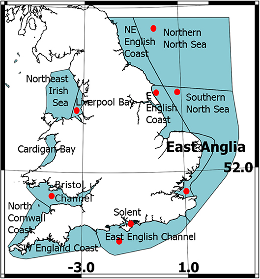
Figure 1. Areas assessed in England and Wales for OSPAR COMP2. The red dots indicate areas where the full COMP2 was applied. East Anglia is highlighted for being the focus area of this paper.

For this study, we selected one of the assessed areas—East Anglia—where an extensive dataset was available. Only the data within this geographical region were analyzed here.

Datasets for the OSPAR COMP2 Assessment

The description of all the datasets used for the OSPAR COMP2 in East Anglia, together with the assessment itself, is given in OSPAR (2008). The available datasets for DIN and chlorophyll were taken from across the UK estuarine, coastal, and offshore monitoring programs.

Datasets for Winter DIN

Three different datasets were available for winter DIN:

• Data collected by the UK Environmental Agency following the requirements of the WFD. Notation wfd was used to refer to this ship-based dataset.

• Data provided by CEFAS to the UK National Marine Monitoring Programme (NMMP). This dataset was named sap to refer to the internal CEFAS database “Sapphire” that contained these data before migration to a more modern system. It is a ship-based dataset.

• Data from the CEFAS Warp SmartBuoy, located in the Thames. This constitutes the only high frequency data record (mean daily values were used for this assessment) of the three sets considered. Details on the SmartBuoy sampling methods and the accuracy of this dataset can be found in Mills et al. (2003); Greenwood et al. (2010) and Johnson et al. (2013). Notation sbu was used for this dataset.

Figure 2A shows the spatial distribution of all data used for the DIN assessment in East Anglia. Estuarine waters (salinity <30) and inshore coastal waters are mainly covered by the wfd dataset, whereas sap and sbu mainly cover the coastal (salinities ≥30 and <34.5) and offshore water bodies (salinity ≥34.5). Figure 2B represents the distribution in time (along the assessment years) of the available datasets. The distribution of data was not homogeneous over time, with 2002 and 2004 better represented than the rest of the years, and 2005 being especially poor in terms of data availability. Focusing on the different datasets, the number of observations from wfd was highest for 2001, 2002, and 2004, but it is very variable along time and very scarce in 2005. The sbu dataset is quite homogeneous in time, and it is the most important dataset in 2003 and 2005. The sap dataset is the smallest of the three.

FIGURE 2

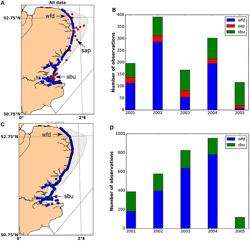
Figure 2. Datasets for the DIN and chlorophyll assessment of East Anglia (COMP2). (A) Spatial distribution of DIN observations. (B) Temporal distribution of DIN observations per year and dataset. (C) Spatial distribution for chlorophyll observations and (D) temporal distribution of chlorophyll observations per year and dataset.

Datasets for Growing Season Chlorophyll

WFD and Warp SmartBuoy data were available for assessments of growing season chlorophyll. The spatial coverage of these datasets did not extend to the full assessment area, with data mainly confined to the coast (Figure 2C). The temporal distribution of the data was not homogeneously distributed between the assessment years (Figure 2D): the number of observations was highest in 2004 and lowest in 2005. The wfd dataset showed an increase in the number of observations between 2001 and 2004, and dropped to zero in 2005. The sbu dataset was quite homogeneous along time.

Additional Datasets

For the assessment of chlorophyll, two additional datasets were explored:

• The Cuxhaven-Harwich FerryBox chlorophyll data ¹. This ferry line was operative in the period 2002–2005. It was the first Ship of Opportunity in which a FerryBox system was installed (see Petersen et al., 2011). Continuous data (temperature, salinity, chlorophyll, oxygen saturation, and pH, nutrients, etc.) were recorded en-route at a temporal resolution of ~20 s, which corresponds to a data point every 550 m, on average. In order to reduce the number of observations and the spatial and temporal autocorrelation, the data were averaged considering a time interval of 10 min, which reduced the spatial resolution to a data point every 3.6 km on average, with a total number of 3,278 observations in the assessment period. Sensitivity analysis were carried out to investigate the effect of the averaging period (1 min, 10 min, 30 min, and 60 min) on the assessment results (only for the aggregation scenario wfd+fbx described below). We will use the notation fbx to refer to this dataset.

• The MODIS daily chlorophyll satellite images. Daily composites of chlorophyll data captured by the MODIS-aqua sensor and processed at IFREMER with the OC5 algorithm (Gohin et al., 2002) were available at a horizontal resolution of 1.1 km during the period 2002–2005. In order to assign a value of salinity to each satellite chlorophyll observation, the results of a model that covered the assessment area were considered. In this way, the modeled salinities were interpolated at the positions of the satellite observations on a daily basis. Details of the model setup and its validation can be found in van Leeuwen et al. (2015) or Ford et al. (2017). The satellite chlorophyll data are called sch throughout this paper, and comprise a total number of 419151 observations for the assessment period, which is more than two orders of magnitude higher than the number of observation used for the OSPAR COMP2 assessment of chlorophyll (see Figure 2D).

Statistical Techniques for the OSPAR COMP2 Assessment

Statistical Techniques for the Assessment of DIN and Chlorophyll

Table 1 summarizes the assessment statistics together with the thresholds applied to the two indicators considered in this paper. The mean winter DIN was normalized to salinity to account for the gradients caused by river inputs that affect the nutrient concentrations. In the OSPAR COMP2, mixing diagrams were used to assess the winter concentrations of DIN (with winter defined as the months of January, February, November, and December of the same year) during the period 2001–2005 (see Foden et al., 2011). The mixing diagrams are used to plot concentrations of DIN against salinity each year, and to calculate linear regressions (Figure 3). All ranges of salinities (from estuarine to offshore) are considered to construct the mixing diagrams. From the linear regression equations, a normalized mean nutrient concentration is calculated for reference salinities for coastal and offshore waters of 32 and 34.5, respectively. Finally, the normalized mean values are compared against the defined salinity-normalized nutrient thresholds.

TABLE 1

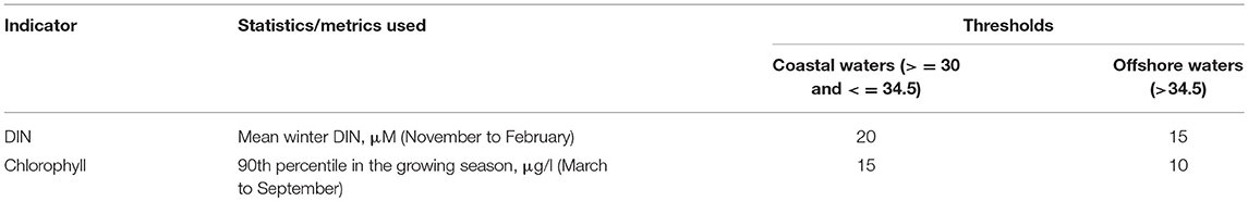
Table 1. Statistics applied to DIN and Chlorophyll and assessment thresholds.

FIGURE 3

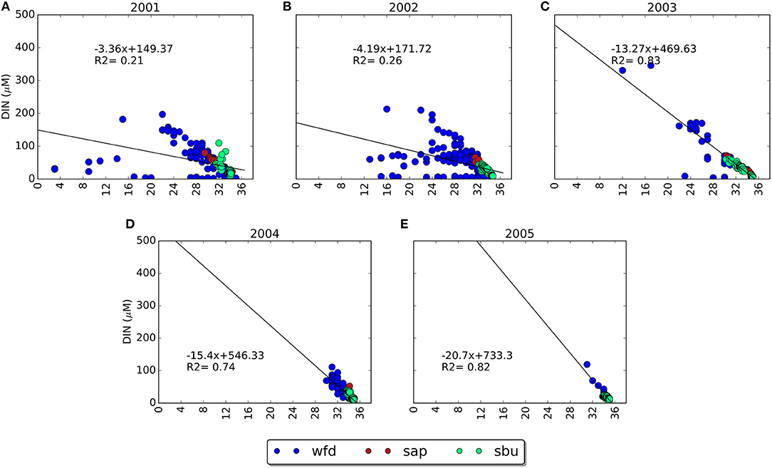
Figure 3. Mixing diagrams and linear regression adjustment for DIN in East Anglia (OSPAR COMP2), years 2001 to 2005 (A–E).

Chlorophyll is assessed using the 90th percentile value during the growing season owing to the distribution of chlorophyll data. The 90th percentile value of the data accounts for the variability and skewness of data associated with episodic high bloom periods and sampling frequency (see Devlin et al., 2007; OSPAR, 2008; Foden et al., 2011).

These statistics were only applied when more than 5 observations were available in any time period being assessed (per year, or for the whole assessment period), as was done in Foden et al. (2011) and OSPAR (2008).

Estimating Confidence

Three measures of confidence were used/applied in this paper:

a) Confidence in the representativeness of the data

b) Confidence in the metrics

c) Confidence relative to the threshold

All three measures combined give information on the confidence in the assessment. Most of the methods that will be described hereafter are different from those employed in the OSPAR COMP2, and are mainly based on the guidelines published in Annex 8 of OSPAR (2013). It is not the purpose of this paper to compare the confidence obtained using these methods with those published in the OSPAR COMP2, but to have a measure that allows for a comparison of the effect on a modern assessment of the different optimization scenarios that were applied to the data (see section Aggregation scenarios).

Confidence in the Representativeness of the Data

The confidence in the representativeness of the data was analyzed in terms of temporal representativeness, spatial representativeness and number of data points.

The representativeness of the available data in time over the assessment period (2001–2005) was calculated taking into account the methodology described in the guidelines published in Annex 8 of OSPAR (2013) and Brockmann and Topcu (2014). The method does not only account for the temporal coverage of the data, but also for the resolution at which large, fast changes (gradients) are sampled. The idea is that if the gradient is flat, not many measurements are necessary to sample the variability and a gap in the measurements would not result in a significant loss of representativeness. However, if the gradient is steep, we would need a higher frequency of sampling to be able to capture the variability, and a gap would have more weight in reducing the representativeness.

The Brockmann and Topcu (2014) method consists of dividing time and/or space into regular intervals/cells and checking whether all of the intervals have been sampled. If an interval has been sampled, it gets the full confidence of 100/N, with N the number of intervals/cells in which the time/space has been divided. Thus, if all the intervals/cells have been sampled, the final representativeness is 100% ($\sum _1^{N}100/N$).

If an interval is not sampled, it gets a reduced score that depends on the difference in gradient between the next sampled cells (calculated as a percentage of the overall gradient) and the number of connected empty cells. In general, the representativeness of an empty interval is given by:

$\begin{array}{ll}R=OR-G*n*\frac{OR}{100}& (1)\end{array}$

with R the representativeness of the empty interval (%), OR the full representativeness of the interval (%), n the number of empty intervals, and G the maximum difference between min-max values of the nearest sampled cells divided by the overall difference in min-max (in %). This is a slight modification of G with respect to Brockmann and Topcu (2014) and follows Annex 8 of the guidance (sections B1 and B2, OSPAR, 2013). If R is negative, it is assigned a score of 0, since it is not contributing to the overall representativeness. For this study, the width of the temporal intervals for the calculation of the temporal representativeness was chosen to be 1 month. Notice that, since we evaluated the temporal representativeness only for the winter months for DIN (January, February, November, and December) and the growing season for chlorophyll (March to September), the empty intervals for which the closest available data were located more than 6 months appart were assigned a score of zero to avoid calculating gradients with data corresponding to different years.

The spatial representativeness was assessed by dividing the assessment area into 1 × 1 km grid cells and counting the number of cells that were occupied by observations from the different dataset combinations and dividing this result by the total number of grid cells in the polygon corresponding to the assessment area for the whole assessment period. The results are also given as a percentage. In this case, the gradient steepness was not considered in the calculation of the spatial representativeness. Note that the results are expected to depend on the selected temporal/spatial discretization.

Confidence in the Metrics

We can provide a confidence rating of the statistics/metrics by calculating the uncertainty associated with the metrics used in the assessments (averages, percentiles, etc.). In general, the uncertainty of the metrics will increase with the variability of the observations and decrease with an increasing number of observations. In the present paper, each metric has an associated 95% confidence interval, which was considered as a proxy for the uncertainty.

Differences in the confidence in the metrics of the aggregation scenarios with respect to the actual OSPAR COMP2 assessment, which will be called the reference assessment from now on, were calculated by considering the change in the width of the 95% confidence intervals.

Confidence Relative to the Threshold

In order to limit the risk of mis-classification as non-problem area, a metric is provided to estimate the confidence level with respect to the threshold. Sections A5 and A6 of Annex 8 in OSPAR (2013) provide different methods to calculate the confidence in the classification depending on whether assessments are based on means or on percentiles.

For assessments based on means (i.e., DIN), two methods are considered:

1. Calculation based on a fixed confidence level (e.g., 90 or 80%). The test consists of calculating the upper 90% (or 80%) confidence limit (using a one-sided t-distribution) and checking if the obtained value is below the reference threshold. If this is the case, then we can answer YES with a 90% (or 80%) confidence to the question: Is this a non-problem area?

2. Calculation based on a variable confidence level. In this case we need to calculate “the largest a priori chosen confidence level that would lead to the conclusion that the test values are below the classification limit.” In other words, in this case we provide the width of the confidence interval (which is the difference between the threshold value and the mean) and we need to calculate the confidence level, which is done by means of the survival function considering a one-sided t-distribution.

In the case of assessments based on percentiles (i.e., chlorophyll assessment), the confidence is calculated as the cumulative probability of the binomial distribution:

$\begin{array}{ll}Cumulativeprobability:P\left(x<k\right)={\displaystyle \sum _{x=0}^{k-1}}\left(\frac{n}{x}\right){\left(\frac{p}{100}\right)}^x{\left(1-\frac{p}{100}\right)}^{n-x},& (2)\end{array}$

where n is the total number of observations, k are the observations below the threshold, which is defined by the p percentile (90th percentile in our case).

This cumulative probability is the confidence level for the conclusion that the p percentile is less than value number k. Consequently, if k of n observations are below the classification limit, this confidence level also applies to the conclusion that the p percentile is less than the classification limit (OSPAR, 2013).

The Optimization Approach

As an initial step toward the optimization of the monitoring systems, we applied heuristic techniques to assess the observational system that was used for OSPAR COMP2, although they can be easily extended to other assessments. The techniques consisted of analyzing several scenarios of aggregation of the available datasets (see sections Datasets for winter DIN and Datasets for growing season chlorophyll) for each of the studied variables (DIN and Chlorophyll). In addition, alternative datasets provided by different observational platforms were available for chlorophyll (FerryBox and satellite data) for the period 2001–2005, allowing for an analysis of the impact on the assessment of using higher spatial- and temporal- resolution datasets. Using additional datasets like FerryBox or satellite chlorophyll involves merging data from different sensors that are not necessarily cross-validated. For this reason, we have carried out a cross-validation exercise among the different datasets to give a quantitative evaluation of the existing mismatch. Finally, all the aggregation scenarios were compared to the reference assessment.

Aggregation Scenarios

For DIN

Of the three datasets considered for the DIN assessment (see section Datasets for winter DIN), two are operated by Cefas: sap and sbu. Therefore, we focused on evaluating the importance of these two datasets. The scenarios were:

• Assessment of individual datasets: this scenario gave an idea of the influence of each dataset in the final assessment.

• Aggregation of wfd+sap: this scenario was intended to exclude and thus evaluate the importance of the high frequency measurements provided by the SmartBuoy.

• Aggregation of wfd+sbu: in this case, we excluded and thus evaluated the relevance of the sap dataset in the OSPAR COMP2 which contains more points in the offshore area than the other two datasets (see Figure 2).

For chlorophyll

Only two datasets were available for the OSPAR COMP2 assessment of chlorophyll in East Anglia: wfd and sbu. We used two additional datasets to analyze their effect on the assessment: the Cuxhaven-Harwich Ferrybox chlorophyll data and MODIS daily chlorophyll satellite images (see section Additional datasets for more details).

The aggregation scenarios that were studied for chlorophyll were:

• Assessment of individual datasets.

• Aggregation of wfd+fbx, to evaluate if the SmartBuoy data could be replaced by FerryBox data.

• Aggregation of wfd+sch, as above but considering the replacement of the SmartBuoy data by satellite data.

• Aggregation of wfd+sbu+fbx, to study the effect on the assessment of adding FerryBox data

• Aggregation of wfd+sbu+sch, to study the effect on the assessment of adding satellite chlorophyll data.

• Aggregation of wfd+sbu+fbx+sch, to study the effect on the assessment of using both FerryBox and Satellite chlorophyll data.

Cross-Validation Between Datasets

Merging datasets obtained from different sensors requires an analysis of the similarity between the available measurements. In this section we introduce a cross-validation tool quantifying the degree of mismatch between the different datasets compared one by one. The cross-validation tool was applied to all the DIN and chlorophyll datasets and consisted of the following steps: (a) spatial gridding of the study area considering a 1 × 1 km grid, (b) finding the points belonging to two different datasets that coincide in the same grid at the same time (considering a daily resolution), (c) calculation of the number of crossing points, correlation, root-mean square error (RMSE), and standard deviation to determine the matching between datasets.

Metrics for Comparing the Aggregation Scenarios

To analyze the importance of a certain dataset for the eutrophication assessment and, ultimately, to answer the questions posed in the Introduction (see section Introduction), we needed to compare the results of the different aggregation scenarios with a reference which, in this case, was the original OSPAR COMP2 eutrophication assessment. We used the following criterion: an aggregation scenario will be considered “similar to” the reference if the assessment result for the analyzed variable lies within the 95% confidence interval of the reference assessment.

Results

Cross-Validation of the Different Datasets

For DIN, all the space/time matchings between wfd and sap, wfd and sbu, and sap and sbu occurred in the Thames estuary adjacent to the Warp SmartBuoy in accordance with the distribution of DIN observations in Figure 2A.

All chlorophyll data locations, including the additional datasets, are given in Figure 4A. The positions of the space/time matchings for chlorophyll between wfd and sbu, wfd and sch, sbu and sch, and fbx and sch, are shown in Figures 4B–E, respectively. No space/time matching between wfd and fbx and sbu and fbx were found.

FIGURE 4

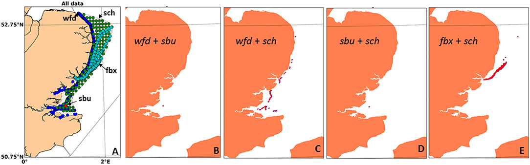
Figure 4. (A) Datasets for the chlorophyll assessment of East Anglia (COMP2) together with the two additional datasets: FerryBox (fbx) and satellite chlorophyll (sch) explored in the scenario testing (see section Aggregation scenarios). (B–E) Space and time matching between the different datasets.

The statistics for all these matchups were represented by means of normalized Taylor diagrams (Taylor, 2001, see Figure 5). The number of matchups for each dataset combination is also included.

FIGURE 5

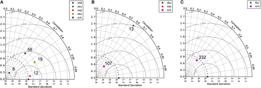
Figure 5. Taylor diagrams showing the statistics of the cross validation between the different datasets. (A) Statistics for the cross validation of wfd with sbu and sap for winter DIN (circles) and of wfd with sbu and sch for chlorophyll (squares). (B) The same for sbu with sap for winter DIN (circle), and sbu with sch for chlorophyll (square). (C) Cross validation of fbx with sch. The number adjacent to each point represents the number of matching points for each cross validation.

For DIN, all dataset combinations were positively correlated (>50%, see the circles in Figures 5A,B), but with a low number of matching points and, especially in the case of the comparison between sbu and sap, different variability, and high RMSE. In the case of chlorophyll, the number of matchups was reasonably high for all the cross-comparisons, except for wfd and sbu, which had only 19. The worst statistics were obtained for the cross validation of wfd and sch (see Figure 5A). The number of matchups in space was quite large with respect to the total number (56 crossing points), meaning that very few data points matched at different times at the same location. The opposite happened for the cross-validation of sch with sbu, which represented a unique point in space for which a large number of temporal matches occurr. In this case, better matching statistics were obtained compared to wfd and sch (compare the purple square in Figure 5B with the same in Figure 5A). The comparison of fbx and sch (Figure 5C), with the largest number of matching points, resulted in a slightly higher RMSE than for the cross validation of sbu with sch, but the representation of the variability was better, with a similar correlation.

Reduced Sampling Scenarios and Use of Additional Datasets

Winter DIN

The results of the OSPAR COMP2 assessment for winter DIN (wfd+sap+sbu), i.e., the reference scenario, and the different aggregation scenarios are given in Table 2 for each of the assessment years and the whole assessment period for the coastal and offshore regions in East Anglia. The confidence in the metrics and confidence relative to the thresholds were reported by the 95% confidence interval and the confidence in the threshold column, respectively, for each of the water types (coastal/offshore) and each of the aggregation scenarios.

TABLE 2

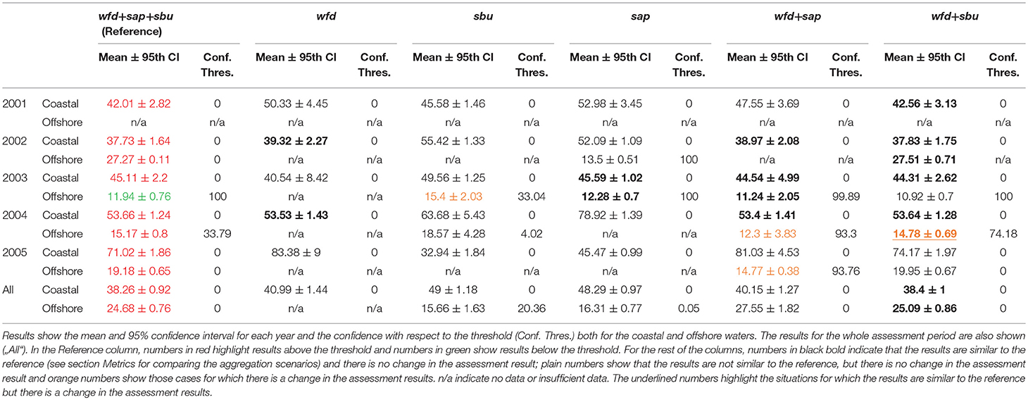
Table 2. Results of the OSPAR COMP2 assessment for winter DIN for the original dataset (Reference) and the different aggregation scenarios.

A representation of the assessment results and the confidence in the metrics is shown in Figure 6A (coastal waters) and Figure 6B (offshore waters), where the impact of aggregating the different datasets is clearly seen.

FIGURE 6

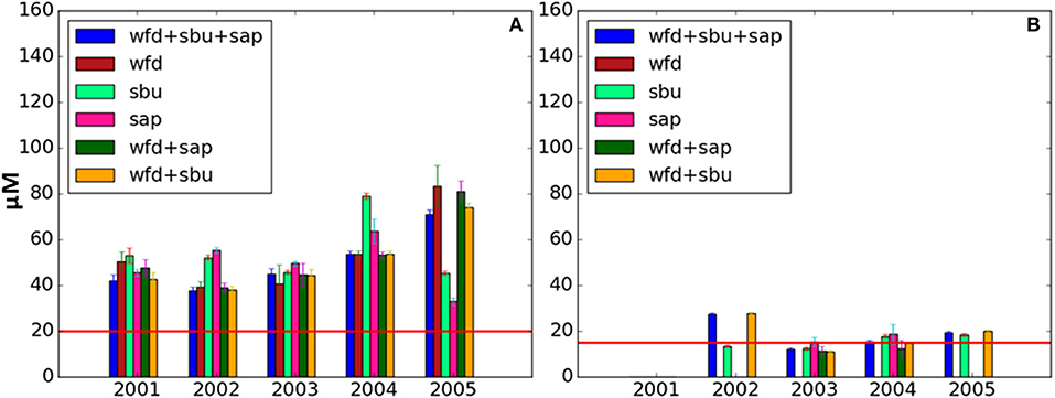
Figure 6. Bar plot showing the results of the OSPAR COMP2 assessment for DIN in coastal waters (A) and offshore waters (B) together with the 95th confidence intervals. Each bar represents one of the analyzed data aggregations given in section Aggregation scenarios. The red line shows the assessment threshold.

The confidence in the representativeness of the data used to produce the assessment results is summarized in Table 3, with Figure 7 showing the number of available data for the reference and the aggregation scenarios in the selected temporal intervals (see Figure 7A). This figure also shows an illustration of the monthly averaged, minimum and maximum time series for the reference and the wfd aggregation scenarios (see Figure 7B), which gives an idea of the steepness of the gradients. The shaded areas correspond to the gaps in the wfd dataset. The scores (in percentage) for each of the time intervals of the wfd dataset following Brockmann and Topcu (2014) (see section Estimating confidence) are plotted in Figure 7C. Notice that the gaps for November and December 2003 are assigned a score zero because the closest available observations correspond to February 2003. In this case, the calculation of a gradient between February 2003 and January 2004 to produce a reduced score would not be meaningful. The same argument was applied to assign a score zero to December 2014. The total temporal representativeness for wfd in Table 3 is the result of summing the percentages for all the temporal intervals in Figure 7C.

TABLE 3

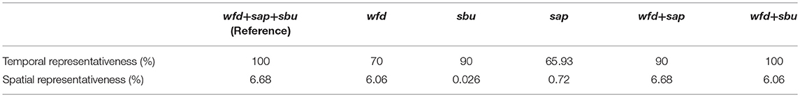
Table 3. Temporal and spatial representativeness of the winter DIN reference dataset and all the aggregation scenarios.

FIGURE 7

Figure 7. (A) Temporal coverage: number of data per time interval of the DIN reference dataset and all the aggregation scenarios. (B) Monthly averaged time series of winter DIN concentration (solid line), and minimum and maximum monthly values (dashed lines) for the reference dataset and aggregation scenario wfd. (C) Representativeness score of each temporal interval following Brockmann and Topcu (2014). Since the number of intervals is 20, the maximum score per interval is 5% (100/20). The scores for the reference (wfd+sap+sbu) are not included because all the intervals get the maximum score.

A summary of the changes of the different scenarios with respect to the reference assessment is given in Table 6.

The reference assessment for DIN—wfd+sap+sbu—was characterized by good temporal representativeness (100%) and not so good spatial representativeness (6.06%, see Figures 2A, 7A). However, the number of observations was not homogeneous over time (see Figure 7A, blue bars), with good coverage in 2002 and few data in 2005, or space (see Figure 2A), with higher coverage closer to the coast and in the Thames Estuary.

The results of the assessment for the coastal region are shown in Table 2 and Figure 6A. The assessment threshold was exceeded in all years and over the whole assessment period. In offshore waters (Table 2 and Figure 6B), the mean did not exceed the threshold in 2003. The assessment for the whole period also indicates that the threshold was exceeded. For all the years and the overall assessment, the confidence in the metrics was relatively high, as indicated by the small confidence intervals.

All the considered reduction scenarios led to overall assessment results for DIN that were aligned with the reference assessment for both the coastal and offshore waters (see Table 6). Only in the case of the aggregation scenario wfd+sbu were overall results within the 95% confidence interval of the reference assessment (see Tables 2, 6 and Figure 6). In other words, only wfd+sbu led to overall results similar to the reference in the sense of section Metrics for comparing the aggregation scenarios. On a year-to-year basis, wfd+sbu also provided similar results to the reference for all the years except 2005 in the coastal waters (the year for which less data were available, see Figure 7A), and for all years except 2003 and 2005 in the offshore waters. Notice that, although the results are similar to the reference in 2004 for offshore waters in the sense of section Metrics for comparing the aggregation scenarios, there is a change with respect to the assessment results, leading to non-exceedance. This aggregation scenario (wfd + sbu) slightly reduced the confidence in the metrics (<10% for coastal waters and <13% in offshore waters) but the spatial and temporal representativeness remained almost unchanged.

For the rest of the aggregation scenarios there was an important reduction (>28%) in the data representativeness (either in time or space) and/or in the confidence in the metrics, implying that some of the relevant spatio/temporal scales have been lost. However, there were still periods of time when certain datasets presented coverage in time and space similar to the reference assessment (see Figures 2A, 7A), and hence similar results coincident with these periods of high data coverage. These were 2002 and 2004 for the coastal waters in scenario wfd, 2003 for the coastal and offshore waters with sap and 2002, 2003, and 2004 for the coastal waters, and 2003 for the offshore waters with wfd+sap.

Chlorophyll

Table 4 gives the results of the OSPAR COMP2 assessment for chlorophyll (wfd+sbu) and for all the aggregation scenarios. It is interesting to notice that, given that the assessment for chlorophyll is based on a percentile (90th percentile), the 95% confidence intervals are not symmetrical, so we provided the width of the lower and upper confidence intervals. Figures 8A,B depict the results of the assessment for the coastal and offshore waters, respectively. The confidence in the representativeness of the data used for the assessment is summarized in Table 5 (plots not shown).

TABLE 4

Table 4. Results of the OSPAR COMP2 assessment for chlorophyll for the original dataset (Reference) and the different aggregation scenarios.

FIGURE 8

Figure 8. Bar plot showing the results of the OSPAR COMP2 assessment for chlorophyll in coastal waters (A) and offshore waters (B) together with the 95% confidence intervals (notice that the confidence intervals are not symmetrical because they are confidence intervals of percentiles). Each bar represents one of the analyzed data aggregations given in section Aggregation scenarios. The red line shows the assessment threshold.

TABLE 5

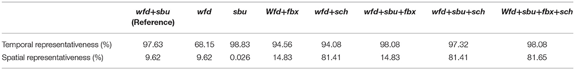
Table 5. Temporal and spatial representativeness of the chlorophyll reference dataset and all the aggregation scenarios.

The reference dataset—wfd+sbu—showed good representativity in time (97.63%), although the representativeness in space was <10% (see Table 5). The sbu dataset was spread quite homogeneously in time, and it was the only available dataset in 2005. On the other hand, wfd presented high variability in terms of number of data points, with 2004 the year for which more data were available (e.g., see Figure 2D). The results of the assessment for the coastal regions are shown in Table 4 and Figure 8A. The assessment threshold was exceeded for all the years in the combined period, except for 2005, with very low confidence relative to the threshold (<16%). An exceptionally high value was obtained in 2004, due to intensive sampling in June 2004 coinciding in time and space with a massive phytoplankton bloom at the northern part of the East Anglia region (see Figure 9). For offshore waters, the results never exceeded the threshold, during the whole assessment period, with very high confidences relative to the threshold.

FIGURE 9

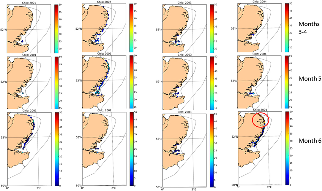
Figure 9. Spatial distribution of chlorophyll observations in time for different assessment years. The red circle shows where the strongest bloom was captured in June 2004.

For chlorophyll, the reduction scenarios consisted of analyzing the individual datasets that comprised the reference scenario (wfd and sbu). In the case of wfd, the overall results of the assessment were aligned with the reference, although not providing similar results in the sense of section Metrics for comparing the aggregation scenarios (see Table 6). Removing the sbu dataset led to a decrease in the temporal representativeness (30%), and reduced the variability of the dataset, causing an increase in the confidence in the metrics (65%). Wfd alone produced similar results to the reference in years 2002, 2003, and 2004 in coastal waters, and in 2002 and 2003 in offshore waters (the only 2 years for which the number of data was enough to carry out the assessment), but led to a result different to the reference in years 2001 and 2003 in coastal waters (no threshold exceedance vs. threshold exceedance in the reference assessment, see Table 4 and Figure 8).

TABLE 6

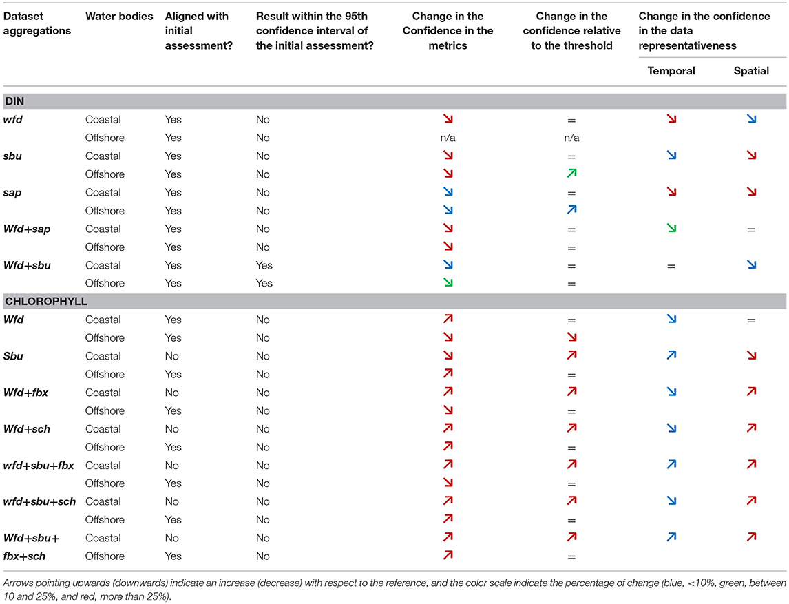
Table 6. Summary of the changes with respect the reference assessement of the different aggregation scenarios.

Using the sbu dataset alone resulted in a change in the assessment results for coastal waters (the threshold was not exceeded), but not for offshore waters. In the latter case, the results were not similar to the reference according to section Metrics for comparing the aggregation scenarios (see Table 4). It was not surprising that removing the wfd dataset had more impact in the coastal waters, because most of the samples were collected in this water body (see Figure 2). The associated loss in spatial representatitivity was high (see Table 5). Sbu data alone could produce results similar to the reference assessment for years 2003 and 2005 in coastal waters (we recall that for 2005 it was the only available dataset), and 2003, 2004, and 2005 in offshore waters, but the results were different for 2002 and 2004 in coastal waters (see Table 4 and Figure 8). Notice that the years for which the sbu results were different to the reference assessment are the same as those for which wfd alone produced similar results, meaning that for these years, only wfd was covering the relevant spatio/temporal scales.

The rest of the studied scenarios for chlorophyll consisted of the utilization of additional datasets. For all these scenarios the results of the overall assessment in coastal waters were opposite to the reference assessment, always resulting in no threshold exceedance. On the contrary, the offshore waters were aligned with the results of the reference assessment, although never within the 95% confidence interval (see Tables 4, 6 and Figure 8). In all the cases, the inclusion of additional datasets led to an increase in the spatial representativity (>25%), in the confidence in the metrics (>65%, mostly in coastal waters) and in the confidence relative to the threshold (>99%, see Table 6), and only a slight change in the temporal representativeness.

All scenarios that included sch (wfd+sch, wfd+sbu+sch, and wfd+sbu+fbx+sch) were biased to this dataset for being the biggest one, and all of them produced opposite results to the reference assessment for years 2002, 2003, and 2004 in coastal waters, and only similar results to the reference assessment for year 2004 in offshore waters (see Table 4).

When sbu was replaced by fbx (scenario wfd+fbx), the results were similar to the original assessment in 2004 for offshore waters. If fbx was combined with the original dataset (wfd+sbu+fbx), years 2004 and 2005 became similar to the reference in the offshore waters, although 2002 became different to the reference (no threshold exceedance) in the coastal waters. It is important to notice that no fbx data were available for years 2001 and 2003 and that the results in Table 4 were obtained considering an averaging interval of 10 min for the fbx data. The results of a sensitivity test for aggregation scenario wfd+fbx showed that different averaging intervals led to different assessment results. In general terms, the shorter the averaging interval, the lower the 90% percentile values. For example, different averaging intervals for coastal waters resulted in 90th percentiles for the chlorophyll assessment of 6.2 (1 min average interval), 13.2 (10 min average interval), 21.9 (30 min average interval), and 30.4 (60 min average interval), compared with the 33.76 value of the reference assessment (see Table 4). It was beyond the scope of this paper to investigate the most appropriate averaging interval that guarantees that all temporal and spatial autocorrelations are removed, and should be the subject of further research.

Discussion

The consideration of different dataset aggregation scenarios can test if different scales of eutrophication monitoring effort can deliver similar results without significantly affecting confidence and representativeness in assessments. These reduced scenarios can provide cost efficiencies but need to be considered in terms of the adequacy of the reduced datasets. Here we discuss the various options using the questions posed in the Introduction.

What Impact Does Each Dataset Have on the Results? i.e., Would We Obtain the Same Assessment Results if We Excluded the SmartBuoys (sbu) or the Ship-Based Sampling (sap)?

Winter DIN

The outcomes of the winter DIN assessment showed that none of the individual datasets (wfd, sbu or sap) can individually reproduce the results of the OSPAR COMP2 assessment for either single years or the whole period, thus showing that none of them are redundant in the calculation of the assessment statistic (normalized mean). Moreover, either sap or sbu data would be necessary for the assessment of the offshore waters, which is not possible with the wfd data alone, since they cover only the coastal waters.

The availability of estuarine data (covered by the wfd dataset) was crucial for the results of the assessment given the way the normalized means are calculated (see Figure 3). For instance, in 2001 and 2002 (see Figures 3A,B), wfd included low salinity/lower nitrate data, which were less available in 2003 (see Figure 3C). This led to steeper slopes in the mixing diagram in 2003 and, hence, higher values of DIN that reflected a lack of observations, and not necessarily a situation of nutrient enrichment. Similarly, in 2004 and 2005, when no estuarine data were available (Figures 3D,E). The mixing diagrams for years 2001 and 2002 suggest that the salinity/DIN gradients from the estuaries to the offshore waters are strongly spatially variable within the East Anglia region. Therefore, splitting this region into more meaningful areas in terms of river plume dynamics, hydrodynamics, etc. would probably have led to a more realistic eutrophication assessment. Assessment areas delineated based on ecologically relevant typologies (salinity, extent of the river plume, ecohydrodynamic characteristics) have been explored in a detailed case study for the Thames and Liverpool Bay area (Greenwood et al., submitted). Also, the use of smaller assessment areas in inshore coastal waters has been found to provide better information for managers and policy makers (Elliott, 2013). In the most recent UK OSPAR assessment (OSPAR COMP3, UK National Report, 2017), estuarine data were not considered for the calculation of the normalized means, resulting in a more consistent comparison of results from year to year.

Chlorophyll

For chlorophyll only two datasets were available for the OSPAR COMP2: wfd and sbu. As for DIN, neither of them could, on their own, produce similar results to the reference for all years, meaning that both datasets were providing important information to the assessment.

The nature of the variability in chlorophyll maxima in time and space makes chlorophyll difficult to sample, even with continuous sampling devices such as the SmartBuoy. The way the chlorophyll assessment is designed can lead to false non-exceedance results for different reasons. For example:

• A phytoplankton bloom may occur at a specific location and time that may be missed by the monitoring platforms [i.e., a strong bloom was captured in June 2004 but not in any other assessment year (see Figure 9)]

• Even if a bloom was detected by the monitoring network, many other observations could reduce the value of the 90th percentile.

Wider Implications

If the SmartBuoy was removed, although we could get results similar to the original assessment in terms of threshold exceedance, they would not lie in the 95% confidence interval of the reference because of the loss of temporal representativeness. Removing the SmartBouy (data) would save approximately £70 k per year, but would result in an increase in the uncertainty due to the decreased temporal representativeness. This higher uncertainty would result in lower confidence in the assessment outcomes. As an aside, the SmartBuoy programme as a whole contributes to increased scientific knowledge in the area by providing long-term time series on environmental changes, data for satellite, and model calibration and validation, etc. Since 2002, more than 60 peer-reviewed papers have been published using SmartBuoy data.

The removal of the ship-based sampling did not seem to significantly affect the results of the assessment for DIN, except for 2005 in coastal waters, and 2003 offshore (these are water body/year combinations for which data are particularly scarce). A substantial amount of these data is collected during SmartBuoy turn-around cruises, and used to calibrate SmartBuoy observations. Hence, reducing SmartBuoy deployments would also reduce the volume of available ship-based data. In addition to SmartBuoy calibration, this dataset is used for the validation of satellite and FerryBox data.

The conclussions with respect to the relevance of each dataset presented here are only valid for the East Anglia Regional Sea. We cannot anticipate if some datasets would be redundant or not in other assessment areas because of the different dynamics and hence, characteristic spatio-temporal scales. However, the employed methodology is easily and quickly applied to other regions and assessments.

The statistical techniques proposed in this paper allow for a preliminary assessment of the monitoring system based on simple methods. In particular, we are able to evaluate if a dataset is redundant or not. A dataset is redundant if it covers spatio-temporal scales that have already been covered by other available datasets. This information is relevant and constitutes an important step toward the optimization of the monitoring system, but with this methodology we still do not quantify to which extent the relevant spatio-temporal scales have been covered by the available datasets. The calculation of the temporal and spatial representativeness presented in this paper gives a partial idea of the data coverage (notice however that lower values would be expected if they were combined in a 3D matrix: longitude x latitude x time), but not of its effectiveness in covering the relevant scales. More sophisticated statistical techniques, such as the effective coverage and the explained variance (see She et al., 2007; Fu et al., 2011) or assimilative model-based methods (OSEs and OSSEs, see She et al., 2007; Oke and Sakov, 2012; Turpin et al., 2016) could be used for this purpose, although this was beyond the scope of this paper.

Does the Addition of New Platforms (Not Included in the Assessment, Like FerryBox or Satellite Data) Significantly Change the Conclusions of the Assessment?

Added Value

According to the results in section Chlorophyll, when the high frequency platforms are considered in the assessments, either by replacing the SmartBuoys (aggregation scenarios wfd+fbx and wfd+sch) or by combining them with the existing datasets (aggregation scenarios wfd+sbu+fbx, wfd+sbu+sch, and wfd+sbu+fbx+sch), the conclusion of the assessment changes significantly, especially in coastal waters. Indeed, in coastal waters a change in the comparison with the thresholds occurs, leading to non-exceedance results when the assessment reported exceedance. The results are less dramatic in offshore waters, for which the assessments using fbx or sch are similar in some years and, when they are not, at least they do not demonstrate a change in the comparison with the threshold.

The high frequency platforms are providing information at scales that are not covered by the available monitoring. But we need to be able to explain the differences with the reference assessments by identifying the issues with the aggregation of the different data sources and the weaknesses of the assessment tools that are being used for chlorophyll currently.

Data Quality and Quantity Considerations

FerryBox and satellite chlorophyll observations are gathered using different sensors and methodologies from in-situ observations and this is the reason why we cross-validated the different datasets to estimate possible biases that could be affecting the final solution. The cross-validation exercise carried out in section Cross-validation of the different datasets could not give information about the degree of comparability between FerryBox and the in-situ datasets as there were no common points. However, fbx could be compared with sch, resulting in statistics like those for the comparison of the in-situ datasets (see, for instance, the statistics for wfd+sbu vs. fbx+sch in Figures 5A,C). However, according to the information in the FerryBox website², the sensors to obtain the chlorophyll concentrations in the FerryBox (fluorometers) need major improvements to account for the dependence of the measurements on the physiological needs of phytoplankton and on the prior illumination, and this would increase the uncertainty of this dataset. FerryBox data have been collected in recent years by the Research Vessel “Cefas Endeavor,” and calibrated against in-situ observations. These high quality data were not available for the OSPAR COMP2, but they constitute an additional and reliable dataset that can be used for future assessments.

In the case of the satellite chlorophyll, the cross validation exercise showed that its temporal variability is comparable with that of sbu (Figure 5C). However, when we compare the sch dataset with wfd we get high bias and RMSE (see Figure 5A). Most of the matchups between these two datasets (see Figure 4C) are influenced by the Thames river plume, and to a lesser extent, other rivers (Orwell, Stour, Colne, and Blackwater), therefore these results are not surprising, since satellite chlorophyll products tend to perform less well in turbid waters.

In the case of the FerryBox, data are gathered as the ship moves, with a temporal resolution of 20 s. This implies a huge amount of information that would be biasing the assessments to the observations on the FerryBox routes. For our particular study, we decided to average the data using a time interval of 10 min, which considerably reduced the number of data points, and increased their distance. However, this averaging procedure did not guarantee that all the temporal and spatial correlations were removed from the dataset, for which specific investigations would be required.

Satellite chlorophyll observations constituted the largest dataset in terms of combined temporal and spatial coverage. In this paper, we have considered daily products gridded at 1 km resolution. Several problems occur with the merging of satellite observations with other datasets. Firstly, retrieval of Level-2 products in coastal waters, where suspended sediment and CDOM co-occur with phytoplankton, is inherently complicated by the optical complexities of these waters (see Qin et al., 2007; Petus et al., 2010; Prieur and Sathyendranath, 2018). However, advances are being made toward the development of reliable satellite products generated with the appropriate algorithms for the different water types (i.e., the EU funded JMP EUNOTSAT project), which will reduce the current associated uncertainty. Secondly, the huge amount of data can dilute any information from other datasets, which may be more reliable. This raises questions about the accuracy of the classical assessment, and on the influence and interpretation of the statistics used. In this sense, the incorporation of high frequency observations into the assessment might require the consideration of smaller assessment areas or revisiting the actual thresholds, which are based on much less observations. Finally, clouds and other artifacts reduce coverage of the relevant areas, which reduces the availability of data, and may introduce bias toward conditions associated with clear weather.

Conclusions

We conclude that all the in-situ datasets used in the OSPAR COMP2 assessment were relevant to replicate the results of the initial assessment, with almost no margin to reduce costs without increasing the uncertainty in the eutrophication assessments and impacting on the ability of the data to deliver the OSPAR assessment requirements. The only case in which a reduction was acceptable was aggregation scenario wfd+sbu for the DIN assessment, since the removal of the sap dataset had almost no impact on the confidence representativeness of the data and the confidence in the metrics.

The spatial and temporal coverage and the methods used in the eutrophication assessment were biased toward certain times and locations where the sampling was more intensive. This was evident in the different annual outcomes, such as the DIN assessment in 2002 resulting in a lower assessment value than the consecutive years as more estuarine sites were sampled, or the chlorophyll assessment, that resulted in a higher value in 2004 than all other reporting years due to the sampling of a bloom.

In order to avoid these biases, an in-situ sampling programme which is more homogeneous in time and space would be required, but is not feasible due to cost. The incorporation of remote sensing and model data, which are currently not used in the eutrophication assessments, could provide the required resolution but need to be integrated with the appropriate methods. The aggregation of in-situ, satellite and modeling data offers the appropriate integration of available datasets to ensure cost efficient monitoring programs collecting data at the appropriate frequency. There would be a need for each dataset to account for its own uncertainty.

In this paper we have made an initial merging test between in-situ and satellite chlorophyll data that resulted in big changes in the assessment results. This was caused by the fact that the satellite chlorophyll was a massive dataset that contained many more low chlorophyll values (outside blooms) than high chlorophyll values, which lowered the 90th percentile. This might be an indication that the classical assessment methods should be revisited, but it first requires a more in depth study focused on the best way to aggregate in-situ, remote sensing and model data, which is in preparation (Collingridge et al., in preparation).

Data Availability Statement

The raw data supporting the conclusions of this manuscript will be made available upon request. The datasets will be published on the Cefas Data Hub (https://www.cefas.co.uk/cefas-data-hub/).

Author Contributions

LG-G wrote the manuscript and analyzed the data. JvdM and DS had the original idea and were crucial in the design of the methodology. SP and KC provided the data and helped with the details of the OSPAR COMP assessment and MD provided guidance throughout the process.

Funding

This study was funded by Cefas Seedcorn Project “Optimizing monitoring programmes using model results” (DP381) and part funded through a Service Level Agreement (Defra-funded).

Conflict of Interest Statement

The authors declare that the research was conducted in the absence of any commercial or financial relationships that could be construed as a potential conflict of interest.

Acknowledgments

The authors would like to thank our colleague Jon Barry for his review and comments on the manuscript and for the interesting discussions.

Footnotes

1. ^http://www.ferrybox.com/

2. ^https://www.ferrybox.com/about/sensors/index.php.en

References

Borja, A., Elliott, M., Carstensen, J., Heiskanen, A. S., and van de Bund, W. (2010). Marine management: towards an integrated implementation of the european marine strategy framework and the water framework directives. Mar. Pollut. Bull. 60, 2175–2186. doi: 10.1016/j.marpolbul.2010.09.026

PubMed Abstract | CrossRef Full Text | Google Scholar

Brockmann, U. H., and Topcu, D. H. (2014). Confidence rating for eutrophication assessments. Mar. Pollut. Bull. 82, 127–136. doi: 10.1016/j.marpolbul.2014.03.007

PubMed Abstract | CrossRef Full Text | Google Scholar

Devlin, M., Bricker, S., and Painting, S. (2011). Comparison of five methods for assessing impacts of nutrient enrichment using estuarine case studies. Biogeochemistry 106, 177–205. doi: 10.1007/s10533-011-9588-9

CrossRef Full Text | Google Scholar

Devlin, M., Painting, S., and Best, M. (2007). Setting nutrient thresholds to support an ecological assessment based on nutrient enrichment, potential primary production and undesirable disturbance. Mar. Pollut. Bull. 55, 65–73. doi: 10.1016/j.marpolbul.2006.08.030

PubMed Abstract | CrossRef Full Text | Google Scholar

EC (1991a). Directive of 21 May 1991 concerning urban waste water treatment (91/271/EEC). Off. J. Eur. Commun. L 135, 40–52.

EC (1991b). Council Directive of 12 December 1991 concerning the protection of waters against pollution caused by nitrates from agricultural sources (91/676/EEC). Off. J. Eur. Commun. L 375, 1–8.

Elliott, M. (2013). The 10-tenets for integrated, successful and sustainable marine management. Mar. Pollut. Bull. 74, 1–5. doi: 10.1016/j.marpolbul.2013.08.001

PubMed Abstract | CrossRef Full Text | Google Scholar

EU (2000). Directive 2000/60/EC of the European Parliament and of the Council of 23 October 2000 establishing a framework for community action in the field of water policy. Off. J. Eur. Commun. 327, 1–72. Available online at: http://data.europa.eu/eli/dir/2000/60/oj

EU (2008). Directive 2008/56/EC of the European Parliament and of the Council of 17 June 2008 establishing a framework for community action in the field of marine environmental policy (Marine Strategy Framework Directive). Off. J. Eur. Union 164, 19–40. Available online at: https://eur-lex.europa.eu/eli/dir/2008/56/oj

Foden, J., Devlin, M. J., Mills, D. K., and Malcolm, S. J. (2011). Searching for undesirable disturbance: an application of the OSPAR eutrophication assessment method to marine waters of England and Wales. Biogeochemistry 106, 157–175. doi: 10.1007/s10533-010-9475-9

CrossRef Full Text | Google Scholar

Ford, D. A., van der Molen, J., Hyder, K., Bacon, J., Barciela, T., Creach, V., et al. (2017). Observing and modelling phytoplankton community structure in the North Sea. Biogeosciences 14, 1419–1444. doi: 10.5194/bg-14-1419-2017

CrossRef Full Text | Google Scholar

Fu, W., Høyer, J. L., and She, J. (2011). Assessment of the three dimensional temperature and salinity observational networks in the Baltic Sea and North Sea. Ocean Sci. 7, 75–90. doi: 10.5194/os-7-75-2011

CrossRef Full Text | Google Scholar

Gohin, F., Druon, J. N., and Lampert, L. (2002). A five channel chlorophyll concentration algorithm applied to SeaWiFS data processed by SeaDAS in coastal waters. Int. J. Remote Sens. 23, 1639–1661. doi: 10.1080/01431160110071879

CrossRef Full Text | Google Scholar

Greenwood, N., Parker, E. R., Fernand, L., Sivyer, D. B., Painting, S. J., Kröger, S., et al. (2010). Detection of low bottom water oxygen concentrations in the North Sea; implications for monitoring and assessment of ecosystem health. Biogeosciences 7, 1357–1373. doi: 10.5194/bg-7-1357-2010

CrossRef Full Text | Google Scholar

Guinehut, S., Larnicol, G., and Le Traon, P. Y. (2002). Design of an array of profiling floats in the North Atlantic from model simulations. J. Mar. Syst. 35, 1–9. doi: 10.1016/S0924-7963(02)00042-8

CrossRef Full Text | Google Scholar

Johnson, M. T., Greenwood, N., Sivyer, D. B., Thomson, M., Reeve, A., Weston, K., et al. (2013). Characterising the seasonal cycle of dissolved organic nitrogen using Cefas SmartBuoy high-resolution time-series samples from the southern North sea. Biogeochemistry 113, 23–36. doi: 10.1007/s10533-012-9738-8

CrossRef Full Text | Google Scholar

Meyers, G., Phillips, H., Smith, N., and Sprintall, J. (1991). Space and time scales for optimal interpolation of temperature — Tropical Pacific Ocean. Prog Oceanogr. 28, 189–218. doi: 10.1016/0079-6611(91)90008-A

CrossRef Full Text | Google Scholar

Mills, D. K., Laane, R. W. P. M., Rees, J. M., et al. (2003). “Smartbuoy: a marine environmental monitoring buoy with a difference,” in Building the European Capacity in Operational Oceanography, eds H. Dahlin, N. C. Flemming and K. Nittis (Petersson SEBT-EOS Elsevier), 311–316. doi: 10.1016/S0422-9894(03)80050-8

CrossRef Full Text | Google Scholar

North, G. R., and Nakamoto, S. (1989). Formalism for comparing rain estimation designs. J. Atmos. Ocean Technol. 6, 985–992. doi: 10.1175/1520-0426(1989)006<0985:FFCRED>2.0.CO;2

CrossRef Full Text | Google Scholar

Oke, P. R., and O'Kane, T. J. (2011). “Observing System Design and Assessment,” in: Operational Oceanography in the 21st Century, eds A. Schiller and G. B. Brassington (Dordrecht: Springer), 123–151.

Google Scholar

Oke, P. R., and Sakov, P. (2012). Assessing the footprint of a regional ocean observing system. J. Mar. Syst. 105–108, 30–51. doi: 10.1016/j.jmarsys.2012.05.009

CrossRef Full Text | Google Scholar

OSPAR (2008) Second OSPAR Integrated Report on the Eutrophication Status of the OSPAR Maritime Area. OSPAR Eutrophication Series publication 372/2008. OSPAR Commission, London. 107.

OSPAR (2013) OSPAR Agreement 2013-8. Common Procedure for the Identification of the Eutrophication Status of the OSPAR Maritime Area. Supersedes Agreements 1997-11 2002-20 and 2005-3. 67.

Petersen, W., Schroeder, F., and Bockelmann, F. D. (2011). FerryBox - application of continuous water quality observations along transects in the North Sea. Ocean Dyn. 61, 1541–1554. doi: 10.1007/s10236-011-0445-0

CrossRef Full Text | Google Scholar

Petus, C., Chust, G., Gohin, F., Doxaran, D., Froidefond, J. M., Sagarminaga, Y., et al. (2010). Estimating turbidity and total suspended matter in the Adour River plume (South Bay of Biscay) using MODIS 250-m imagery. Cont. Shelf Res. 30, 379–392. doi: 10.1016/j.csr.2009.12.007

CrossRef Full Text | Google Scholar

Prieur, L., and Sathyendranath, S. (2018). An optical classification of coastal and oceanic waters based on the specific spectral absorption curves of phytoplankton pigments, dissolved organic matter, and other particulate materials1. Limnol. Oceanogr. 26, 671–689. doi: 10.4319/lo.1981.26.4.0671

CrossRef Full Text

Qin, Y., Brando, V. E., Dekker, A. G., and Blondeau-Patissier, D. (2007). Validity of SeaDAS water constituents retrieval algorithms in Australian tropical coastal waters. Geophys. Res. Lett. 34:L21603. doi: 10.1029/2007GL030599

CrossRef Full Text | Google Scholar

She, J., Allen, I., Buch, E., Crise, A., Johannessen, J. A., Le Traon, P. Y., et al. (2016). Developing european operational oceanography for blue growth, climate change adaptation and mitigation, and ecosystem-based management. Ocean Sci. 12, 953–976. doi: 10.5194/os-12-953-2016

CrossRef Full Text | Google Scholar

She, J., Amstrup, B., Borenäs, K., Buch, E., Funkquist, L., Luyten, P., et al. (2006). Optimal Design of Observational Networks. FP5th Contract No. EVK3-2002-00082. Available online at: https://cordis.europa.eu/project/rcn/67321/factsheet/en

She, J., Høyer, J. L., and Larsen, J. (2007). Assessment of sea surface temperature observational networks in the Baltic Sea and North Sea. J. Mar. Syst. 65, 314–335. doi: 10.1016/j.jmarsys.2005.01.004

CrossRef Full Text | Google Scholar

She, J., and Nakamoto, S. (1996). Spatial sampling study for the tropical pacific with observed sea surface temperature fields. J. Atmos. Ocean Technol. 13, 1189–1201. doi: 10.1175/1520-0426(1996)013<1189:SSSFTT>2.0.CO;2

CrossRef Full Text | Google Scholar

Smith, N. R., and Meyers, G. (1996). An evaluation of expendable bathythermograph and tropical atmosphere-ocean array data for monitoring tropical ocean variability. J. Geophys. Res. Ocean 101, 28489–28501. doi: 10.1029/96JC02595

CrossRef Full Text | Google Scholar

Taylor, K. E. (2001). Summarizing multiple aspects of model performance in a single diagram. J. Geophys. Res. Atmos. 106, 7183–7192. doi: 10.1029/2000JD900719

CrossRef Full Text | Google Scholar

Turpin, V., Remy, E., and Le Traon, P. Y. (2016). How essential are Argo observations to constrain a global ocean data assimilation system? Ocean Sci. 12, 257–74. doi: 10.5194/os-12-257-2016

CrossRef Full Text | Google Scholar

UK National Report (2017). Common Procedure for the Identification of the Eutrophication Status of the UK Maritime Area. 2017. Available online at: https://www.ospar.org/work-areas/hasec/eutrophication/common-procedure. iv + 201 pp

van Leeuwen, S., Tett, P., Mills, D., and van der Molen, J. (2015). Stratified and nonstratified areas in the North Sea: Long-term variability and biological and policy implications. J. Geophys. Res. Ocean 120, 4670–4686. doi: 10.1002/2014JC010485

CrossRef Full Text | Google Scholar