Oxygen Variability During ENSO in the Tropical South Eastern Pacific

Introduction

Oxygen Minimum Zones (OMZ) are large water bodies of the open ocean with low concentrations of dissolved oxygen (DO < 22 μmol kg⁻¹) at subsurface depths (~50–900 m; Levin, 2003; Karstensen et al., 2008). Low DO has a strong impact on the nitrogen cycle: a significant portion (35%) of the nitrogen loss in the global ocean occurs in these regions (Devol et al., 2006) due to denitrification and anammox (Babbin et al., 2014). The oxycline, which separates the well-mixed surface waters with the low-oxygenated subsurface waters, also impacts marine life by limiting the habitat of several species in the water column (Diaz and Rosenberg, 2008; Gutiérrez et al., 2008; Bertrand et al., 2011). These features, along with the recently observed increase of their vertical extent (Stramma et al., 2008, 2010; Ito and Deutsch, 2013; Schmidtko et al., 2017; Breitburg et al., 2018) have made OMZ studies an oceanographic hot topic in the recent decades.

The OMZ of the Tropical South Eastern Pacific (TSEP; Figure 1) is one of the most intense OMZ of the open ocean (Fuenzalida et al., 2009; Paulmier and Ruiz-Pino, 2009; Ulloa and Pantoja, 2009). DO concentrations in its core can be lower than 5 μmol kg⁻¹ or totally depleted (e.g., Czeschel et al., 2015; Thomsen et al., 2016). Off Peru the OMZ extends vertically between ~50–100 and 600–700 m depth on average (Fuenzalida et al., 2009), being deeper offshore (Karstensen et al., 2008). Near the coast, the oxycline is found at 20–50 m water depth (Graco et al., 2007; Gutiérrez et al., 2008; Fuenzalida et al., 2009).

FIGURE 1

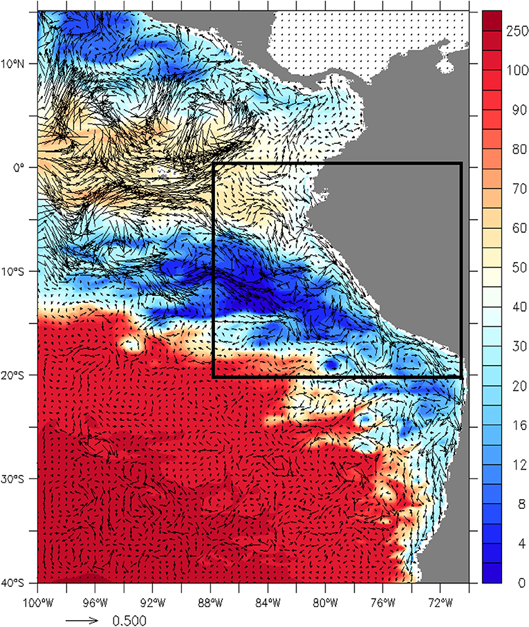
Figure 1. Modeled Velocity current (arrows, in m s⁻¹) and DO mean (color scale, μmol kg⁻¹) between 200 and 300 m depth during December 1997–March 1998. The black box marks the studied area.

Complex physical and biogeochemical processes are involved in the TSEP OMZ formation and maintenance. Vertical mixing between the shallow, oxygenated, surface mixed layer and subsurface OMZ waters is reduced due to the relatively weak alongshore winds. A sharp permanent pycnocline also mitigates vertical mixing and prevents local ventilation of subsurface waters (Fiedler and Talley, 2006). Furthermore, it is located in the poorly ventilated “shadow zone” of the Subtropical South Eastern Pacific, out of reach of the ventilated water masses pathways which subduct in the thermocline (Luyten et al., 1983). Indeed, the residence time of OMZ waters can be very long: water masses may recirculate within the OMZ during more than a year (e.g., ~15 months at 8°S, Czeschel et al., 2011). On the other hand, as it is relatively close to the equatorial region, the northwestern boundary of the OMZ is ventilated by the equatorial current system and is sensitive to its variability. In particular, equatorial subsurface undercurrents (SSCCs) or Tsuchiya jets (Tsuchiya, 1975) transport relatively DO-rich waters eastward (Montes et al., 2014). The nearshore OMZ is then ventilated by the poleward Peru-Chile Undercurrent (PCUC), which connects the offshore equatorial region to the Peruvian coastal upwelling system (PCUS) (Zuta and Guillén, 1970; Codispoti et al., 1989; Chaigneau et al., 2013). The PCUC is recognized as the main source of the upwelling waters (Huyer et al., 1987). It is mainly fueled by the primary (2°S−6°S, pSSCC) and secondary (6°S−10°S, sSSCC) subsurface undercurrents (Montes et al., 2010), and to a much lesser extent by the Equatorial Undercurrent (2°N−2°S, EUC; Wyrtki, 1967). In addition, the TSEP OMZ is embedded in a region of intense mesoscale activity (Chaigneau et al., 2008) due to the presence of unstable boundary currents (Echevin et al., 2011; Colas et al., 2012). These eddies generate horizontal (e.g., Vergara et al., 2016) and vertical eddy fluxes which impact the OMZ structure.

The very high PCUS productivity also impacts the OMZ. The large amount of organic matter (OM) eventually sinks into the OMZ, and oxygen is consumed by microbial respiration during OM remineralization (e.g., Paulmier et al., 2006; Cavan et al., 2017). Overall, the temporal variability of the OMZ extension is assumed to be mainly driven by physical processes (e.g., Xu et al., 2015), but its maintenance is due to the oxygen respiration (Paulmier et al., 2006).

The OMZ is variable over a wide range of temporal and spatial scales. At seasonal time scales, its variability is related to the local wind forcing, remineralization and mesoscale circulation (eddies and filaments; Thomsen et al., 2016; Vergara et al., 2016). At interannual time scales, the OMZ is mainly affected by the warm (El Niño, EN) and cold (La Niña, LN) phases of the El Niño Southern Oscillation (ENSO). During EN, intraseasonal Equatorial Kelvin Waves (IEKW) are generated by wind anomalies in the Equatorial Pacific region (e.g., Kessler et al., 1995). They propagate eastward and reach the western coasts of America. There, they trigger coastal trapped waves (CTWs) which propagate poleward and impact the vertical structure of physical and biogeochemical variables alongshore off Peru (Gutiérrez et al., 2008; Echevin et al., 2014; Graco et al., 2017) and Chile (Ulloa et al., 2001). The water column thus becomes oxygenated during EN and a deeper oxycline (>100 m) is observed (Gutiérrez et al., 2008, 2016), while during LN (e.g., 1999–2000), a shallower oxycline is described (Graco et al., 2007, 2017). These DO changes are strongly linked with the physical variability, as both the thermocline and oxycline are displaced vertically during the passage of downwelling (warm) and upwelling (cold) CTWs (Echevin et al., 2014; Graco et al., 2017).

Besides, the DO content of the PCUC could also be modified during ENSO. As it is fed mainly by the pSSCC and the EUC during LN and by the sSSCC during EN (Montes et al., 2011), variability in DO concentrations in the equatorial region could impact differently the ventilation of the OMZ.

Few modeling works have described the OMZ variability at interannual time scales. Using a regional model, Mogollón and Calil (2017) simulated the impact of the strong 1997–1998 EN and 1999–2000 LN events on the OMZ. They found a deepening (~150 m) of the OMZ during 1997–1998 EN respect to neutral condition, while a shallower OMZ (~50 m) was observed during LN in the main coastal upwelling centers of the PCUS. Using a global model, Yang et al. (2017) found that the denitrifying SETP OMZ core volume expanded during LN (e.g., ~+35% in 1999–2000 LN) and shrinked during EN (e.g., ~-75% in 1982–1983/1997–1998 EN). Note that in these recent works, few in situ oxygen measurements were used to validate the simulations during ENSO.

In the present work, we make use of a unique interannual DO in situ data set and of a regional physical-biogeochemical coupled model to study the physical and biogeochemical processes involved in the OMZ variability during EN and LN phases. Unlike previous studies, we simulated a large number of ENSO events from 1958 to 2008, which allows a comparison of the impact of extreme and moderate events. After carefully evaluating the model with in situ data, we used the model to investigate the role of the CTWs, the impact of the equatorial circulation and the ventilating eddy fluxes due to the variable mesoscale activity during EN and LN events. Finally, we performed sensitivity experiments forced by contrasted atmospheric and open boundary forcing to investigate the impact of the local (e.g., wind and heat fluxes) and remote forcing (e.g., coastal waves) on the DO changes during EN and LN.

Materials and Methods

The ROMS-PISCES Coupled Physical-Biogeochemical Model

The Regional Oceanic Modeling System model (Shchepetkin and McWilliams, 2005) was used to simulate the ocean dynamics. The ROMS-AGRIF code (version 3.1) was used (Penven et al., 2006). ROMS resolves the Primitive Equations, based on the Boussinesq approximation and hydrostatic vertical momentum balance (Shchepetkin and McWilliams, 1998). ROMS is coupled to the Pelagic Interaction Scheme for Carbon and Ecosystem Studies (PISCES) biogeochemical model to simulate the marine biological productivity and the biogeochemical cycles of carbon and main nutrients (P, N, Si, Fe; Aumont et al., 2015) as well as DO (e.g., Resplandy et al., 2012). PISCES has three non-living compartments which are the semi-labile dissolved organic matter, small sinking particles and large sinking particles, and four living compartments represented by two size classes of phytoplankton (nanophytoplankton and diatoms) and two size classes of zooplankton (microzooplankton and mesozooplankton).

This coupled model has been used to study the climatological (Echevin et al., 2008; Albert et al., 2010), intraseasonal (Echevin et al., 2014), and interannual (Espinoza-Morriberón et al., 2017) variability of the surface productivity in the PCUS.

The Oxygen Cycle in the PISCES Model

The oxygen evolution in PISCES is computed taking into account the dynamical transport, biogeochemical processes (sources and sinks) and air-sea fluxes, as follows:

$\partial t{O}_2=\underset{Dynamicaltransport}{\underbrace{-u_H.{\nabla }_H{O}_2-w.{\nabla }_H{O}_2+\frac{\partial K_z\partial O_2}{\partial z^2}}}+\underset{Biogeochemicalprocesses}{\underbrace{{\left(\frac{\partial O_2}{\partial t}\right)}_{Bio}}}+\underset{air-oceanexchange}{\underbrace{J_{flux}}}$

u_H and w represent the horizontal (zonal and meridional) and vertical currents, respectively. K_z represents the vertical diffusivity. The last term on the right hand side represents the air-sea oxygen flux, which depend on the partial pressure air-sea difference, solubility and velocity transfer of oxygen. The atmospheric oxygen concentration is constant throughout the simulation.

Besides, the biogeochemical processes which produce and consume oxygen are parameterized as follows (see also Resplandy et al., 2012):

$\begin{array}{l}{\left(\frac{\partial O_2}{\partial t}\right)}_{Bio}=R_{O/C}^1.\underset{NewProduction}{\underbrace{\left({\mu }_{nh4}^{P}P+{\mu }_{nh4}^{D}D\right)}}+\left(R_{O/C}^1+R_{O/C}^2\right).\underset{RegeneratedProduction}{\underbrace{\left({\mu }_{no3}^{P}P+{\mu }_{n\text{o}3}^{D}D\right)}}\\ -R_{O/C}^1.\underset{RemineralizationandRespiration}{\underbrace{\left({\lambda }_{DOC}^{\text{*}}\left(1-△\left(O_2\right)\right)DOC+G^{Z}Z+G^{M}M\right)}}-R_{O/C}^2.\underset{Nitrification}{\underbrace{Nit}}\end{array}$

Diatoms (D) and nanophytoplankton (P) produce oxygen during photosynthesis through new and regenerated production. The corresponding production rates are μ_nh4 and μ_no3. Oxygen consumption is due to remineralization of Dissolved Organic Carbon (DOC), respiration of mesozooplankton (G^ZZ) and microzooplankton (G^MM), and nitrification. ${\lambda }_{DOC}^{{}^{*}}$represents the remineralization rate. (O₂) varies between 0 (in oxic conditions) and 1 (anoxia), mimicking the suppression of remineralization in anoxic conditions. $R_{\frac{O}{C}}^1$ (131/122) represents the change in oxygen relative to carbon when ammonium is converted to organic matter during new production and when DOC is being respired. $R_{\frac{O}{C}}^2$ (32/122) represents the change in oxygen relative to carbon during nitrification (Nit). More detail about the model structure and parameterizations can be found in Aumont et al. (2015).

Model Configuration

The model domain spanned from 15°N to 40°S and from 100°W to 70°W (Figure 1). Due to the extension of the model area and computational requirements, the horizontal resolution of the grid was 1/6° (~18 km). It allowed to reproduce mesoscale structures off Peru owing to the proximity of the region to the equator (see section Ventilation by Eddy Fluxes). The bottom topography from ETOPO2 (Smith and Sandwell, 1997) was used, and the vertical grid had 32 sigma levels.

Open boundary conditions (OBC) for physical variables came from an interannual SODA model solution (version 2.1.6; Carton and Giese, 2008) over the period 1958–2008. As an interannual global simulation of the biogeochemical conditions was not available during the period of study (1958–2008), climatological OBC from CARS2009 climatology (Ridgway et al., 2002) were used for nutrients (nitrate, silicate, phosphate) and oxygen and from World Ocean Atlas climatology (WOA2005; Conkright et al., 2002) for DOC, dissolved inorganic carbon and total alkalinity. As a gridded climatology of iron measurements does not exist, iron OBC from a climatology of a NEMO-PISCES global simulation were used (Aumont et al., 2015).

Wind stress, fresh water, sensible and latent heat fluxes were computed using the bulk parameterization of Liu et al. (1979). The surface wind fields were obtained by summing statistically-downscaled NCEP daily wind anomalies (Goubanova et al., 2011) and the SCOW monthly climatology (Risien and Chelton, 2008). NCEP daily anomalies and COADS monthly climatology (Da Silva et al., 1994) were summed to obtain surface air parameters. Climatologies of short (COADS) and downward long wave (NCEP) heat fluxes were used. The forcing characteristics of the different simulations are listed in Table 1.

TABLE 1

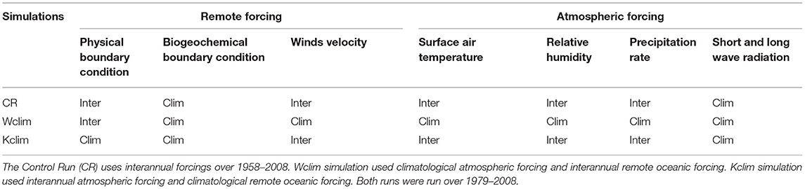
Table 1. Characteristics of the model simulations.

The model was run from 1958 to 2008, the period over which the SODA solution that we use (v.2.1.6) is available. Note that over the last 10 years, there was no occurrence of any strong, or extreme, LN or EN events off Peru. Thus, we are confident that the mean state of ENSO phases evaluated in this work are robust.

Model Experiments

The interannual simulation which is mainly described and studied in the following sections is named the control run (CR). It was forced by interannual atmospheric forcing and boundary conditions. The circulation, productivity and nutrient fluxes during ENSO were evaluated in Espinoza-Morriberón et al. (2017).

Two additional simulations were performed and analyzed (Table 1):

- The Wclim simulation, forced by interannual OBC and monthly climatological atmospheric forcing, was used to evaluate the role of the oceanic remote forcing, e.g., equatorial subsurface currents, equatorial Kelvin waves and coastal trapped waves.

- The Kclim simulation, forced by monthly climatological OBC and interannual atmospheric forcing, allowed to study the role of the wind forcing.

Due to computational requirements Kclim and Wclim were run from 1979 to 2008, a period which included two extreme EN events (1982–1983/1997–1998) and one strong LN event (1999–2000). Five day-averaged outputs were stored for each simulation.

Lagrangian Analysis

The ROMS-offline tracking module (Capet et al., 2004) was used to calculate the trajectories of virtual floats simulating water parcels. The floats trajectories were computed using the 5-day averaged velocity fields. Oxygen concentration were registered along the trajectories. In order to describe the source waters (SW) characteristics reaching the nearshore OMZ, 2000 floats were released over the shelf and slope, between the surface and 350 m depth within ~150 km from the coast on the first day of each month of spring (October, November, December), during each LN and EN events and during neutral periods. The floats were released from a zonal section at 9°S, but other sections (e.g., 12°S) were tested. The floats were then tracked backwards in time during 2 years. The floats reaching the so-called offshore equatorial region (defined by a meridional section at 88°W, 2°N−10°S) were used to compute statistics. The characteristics of these waters (DO concentration and depth in the equatorial region, duration of the transit from the equatorial section to the cross-shore coastal section (at 9°S) were mapped onto the cross-shore section where the water parcels were released (see section Changes in the Origin of the Shelf and Slope Waters During ENSO).

Eddy Fluxes

The oxygen vertical eddy flux was computed as $\overline{w^{\prime }.O_2^{\prime }}=\overline{w.O_2}-\overline{\langle w\rangle .\langle O_2\rangle }$, where w and O₂are the 5 day-averaged vertical velocity and oxygen concentration, respectively. 〈.〉 denotes a moving filter with a 60 days' window. The mean profiles of oxygen mean vertical flux and eddy vertical flux were obtained by averaging values horizontally (horizontal averaging is marked by an overbar) in an offshore box (between 100 and 500 km from the coast and between 6°S and 16°S). We chose to average profiles in an offshore box in order to discard the effect of nearshore upwelling and downwelling velocities associated with the CTWs and to retain the role of eddies and filaments.

The meridional ($v^{\prime }.O_2^{\prime }$) and zonal ($u^{\prime }.O_2^{\prime }$) eddy oxygen fluxes were computed using the same time filter. Maps of the intensity and direction of the horizontal eddy fluxes ($\sqrt{{(u^{\prime }.O_2^{\prime })}^2+{(v^{\prime }.O_2^{\prime })}^2}$) at 100 and 400 m during neutral, LN and EN events are described in section Eddy Oxygen Fluxes.

ENSO Index and Statistical Tests

ENSO phases are defined when the 3-month-running mean SST anomaly in the “Niño1+2” region (0–10°S, 90°W−80°W) is higher or < ± 0.5°C for at least 5 consecutive months for EN and LN, respectively, (as in Espinoza-Morriberón et al., 2017). The ERSST.v4 SST product of Huang et al. (2015) was used. Neutral periods correspond to non-EN and non-LN periods. For EN events, if the SST anomalies are >+ 1.6°C during at least 3 months the event is categorized as “extreme,” otherwise it is a “moderate” EN (see Table in Supplementary Material). The correlation between the Niño1+2 index computed from the model SST and observations was 0.9, thus the majority of EN and LN events were represented by the model.

The non-parametric Wilcoxon test was used to statistically compare the means of some characteristics (e.g., OMZ depth) for EN, LN and neutral period, and to test if these means differ with a 95% confidence level. To compute this test, we used the function “pairwise.wilcox.test” from R software.

Oxygen in situ Observations

Approximately ~20,000 DO vertical profiles collected by the Peruvian Marine Institute (IMARPE) between 1960 and 2008 (Bertrand et al., 2011; Ledesma et al., 2011) were used to evaluate the modeled OMZ. DO was determined by the Winkler method (Carrit and Carpenter, 1966). Observations (Nansen and Niskin bottles) were collected during surveys and at fixed stations along the coast. The data was gridded at the same resolution as the model (1/6°). Composite alongshore-averaged cross-shore sections for neutral and ENSO phases between 6°S and 16°S and 100 km from the coast (hereafter coastal region) were computed.

The depth of the upper limit of the OMZ (i.e., where DO is equal to 22 μmol kg⁻¹) was computed from each IMARPE profile (linearly interpolated on a vertical grid with a 1 meter resolution). These values were then averaged horizontally in the coastal region to produce an index (ZO2) characterizing oxygenation in the nearshore region.

In addition, CARS2009 DO observations (Ridgway et al., 2002) were used to evaluate the spatial distribution of the simulated oxygen over the entire model domain. The CARS 1/2° gridded data was interpolated onto the 1/6° model grid.

Results and Discussions

Evaluation of the Modeled OMZ

Mean State

The mean modeled and observed OMZ are shown in Figure 2. ZO2 presented a marked cross-shore gradient, with shallower depths (<25 m) near the coast than offshore (~100 m at 100 km from the coast off the central shelf). The nearshore ZO2 was deeper in the model (~50–70 m between 6°S and 14°S), than in the observations (~30 m in IMARPE and ~ 50 m in CARS). ZO2 reached 150 m depth at 86°W between 6°S and 14°S (Figures 2a–c), highlighting the offshore deepening and westward extent of the OMZ.

FIGURE 2

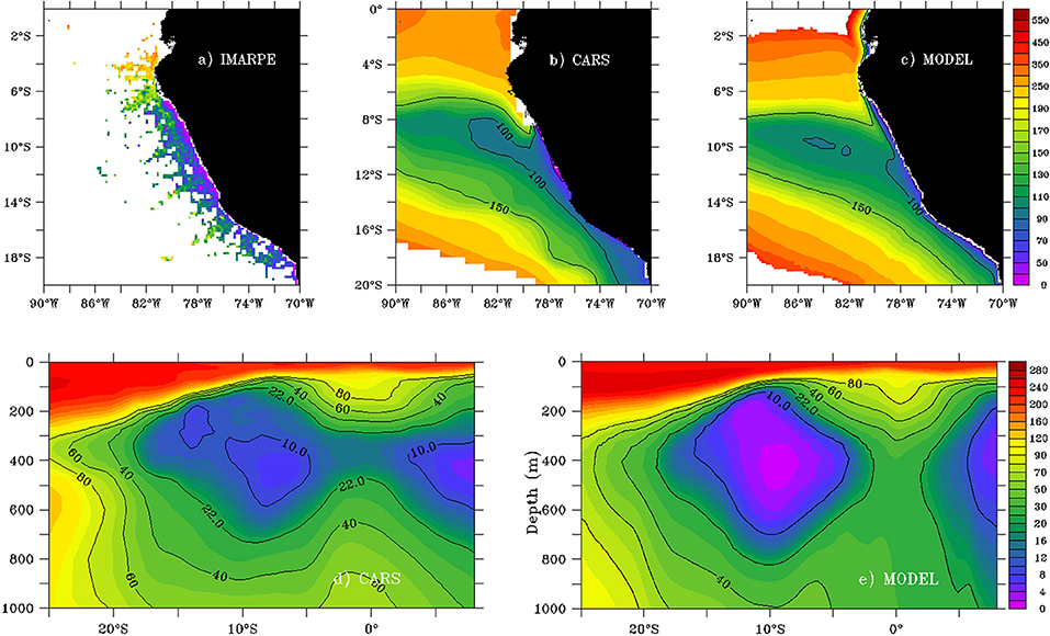
Figure 2. Annual ZO2 mean (in meters) from IMARPE (a), CARS (b) and model (c). Meridional section (86°W) of the annual DO mean (in μmol kg⁻¹) from CARS (d) and model (e). Annual means were computed over 1958–2008 using the model and IMARPE data.

Figures 2d,e display a meridional section of the OMZ at 86°W, more than 1,500 km east of the model western boundary. The modeled and observed OMZ boundaries were rather similar between 6°S and 14°S. Although ZO2 was relatively similar in the model and CARS observations, the maximum OMZ thickness (found near 8°S−10°S at 86°W) was larger in the model than CARS due to the OMZ deeper (by ~100 m) lower limit in the model. In the core of the OMZ between 8°S−11°S and 200–500 m depth, modeled DO concentrations were lower than 5 μmol kg⁻¹, lower than CARS (~10 μmol kg⁻¹). Between 2°S and 2°N the modeled OMZ vanished, while a thin (~100 m) OMZ remained between 300 and 450 m depth in CARS.

Interannual Variability

Due to the relative scarcity of in situ data, it was impossible to compute cross-shore sections of DO at distinct latitudes, therefore we present alongshore-averaged cross-shore sections between 6°S and 16°S (see section Oxygen in situ Observations) representative of averaged DO conditions near the Peru shelf and slope (e.g., Espinoza-Morriberón et al., 2017). The model and data sections are shown for neutral, EN and LN phases (Figure 3). Near-surface slanted isolines of oxygen were evidenced in the model and IMARPE sections during neutral, EN and LN events, indicating the occurrence of coastal upwelling during each phase (Figures 3A–C,F–H). During neutral periods, between the coast and 200 km offshore, the observed ZO2 was located at ~180 m depth and the modeled ZO2 at ~150 m depth (Figures 3A,F). In contrast, during EN (LN) a deeper (slightly shallower) ZO2 was observed in the model (Figures 3B,C). These features were well reproduced by the model (Figures 3G–H). The main differences between model and observations were found in the OMZ core and near its lower limit. In the model, DO values <5 μmol kg⁻¹ were observed in the OMZ core (between 300 and 450 m depth) during neutral and LN periods. During EN, the thickness of lowest DO (<5 μmol kg⁻¹) layer was reduced. In contrast, the observations presented a slightly more oxygenated core than in the model during neutral (~8 μmol kg⁻¹), EN (~15 μmol kg⁻¹), and LN (~12 μmol kg⁻¹) periods. Moreover, the modeled OMZ lower limit was deeper than that of the observed OMZ, in particular during LN (Figures 3C–H). During EN, both observations and model presented a thinner OMZ than during neutral periods, owing to a deepening of its upper limit and a shoaling of its lower limit (Figures 3B,G). In contrast, the model was not able to simulate the observed OMZ thinning during LN. Indeed, the modeled OMZ was thicker during LN with respect to neutral conditions due to little change of its lower limit, whereas the shoaling of the lower limit was strong in the observations.

FIGURE 3

Figure 3. DO (in μmol kg⁻¹) alongshore-averaged (6°S−16°S) vertical sections during neutral, EN and LN periods, from IMARPE data (A–C) and model output (F–H). DO anomaly alongshore–averaged vertical sections (6°S−16°S) for EN and LN periods from IMARPE (D,E) and model output (I–J).

In terms of magnitude, the DO changes in the surface layer (0–150 m) during ENSO phases were qualitatively reproduced by the model. The highest DO anomalies were observed between 10 and 150 m (Figures 3D–I) both in the model (+40 μmol kg⁻¹) and in observations (+25 μmol kg⁻¹) during EN. During LN, negative anomalies of similar amplitude in the model and observations (~-10 μmol kg⁻¹; Figures 3E,J) were found in the same layer between the coast and 150 km offshore.

Interannual variations of the nearshore modeled and observed ZO2 were highly correlated over 50 years (r = 0.72, p < 0.05, Figure 4). During each EN event, ZO2 increased strongly. The maximum ZO2 (~300 m) was attained during the peak of the extreme 1982–83 EN for model and observations. In the model and observation, the ZO2 during Neutral and LN periods did not present statistical differences (p > 0.05); however, both presented significant differences respect to EN event (p < 0.05). During neutral periods, the observed and modeled ZO2 were ~72 m depth on average, while during LN, the oxycline was found at ~60 m for both. In conclusion, in spite of the discrepancies in DO concentration within the OMZ (Figures 3–5), the model represented realistically the oxygen changes during ENSO phases.

FIGURE 4

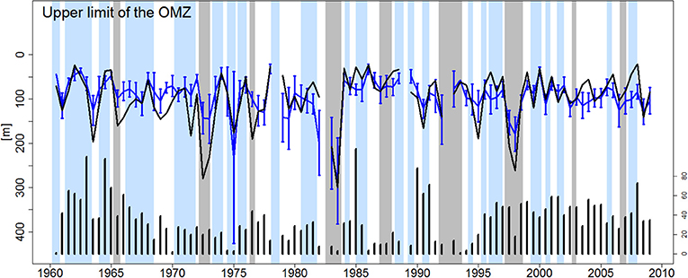
Figure 4. ZO2 time series (in meters). Data was averaged each semester for IMARPE (blue line) and model output (black line) in a coastal box (6°S−16°S and 100 km from the coast). Error bars represent the standard deviation from IMARPE data. Black bars (at the bottom of the figure) represent the coverage ratio (number of sampled points/ total number of points). The modeled ZO2 was computed using the same sampling as IMARPE observations (gaps mean there is no data). Gray and blue shading represent EN and LN period, respectively.

FIGURE 5

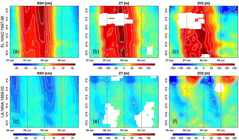
Figure 5. Hovmoller (latitude vs. time) of modeled SSH anomalies (a,d, in cm), ZT15 anomalies (b,e, in meters) and ZO2 anomalies (c,f, in meters) during EN 1997–1998 (top) and LN 1999 (bottom) events. Model values were averaged within 100 km to the coast. All variables were filtered in time (60 days moving average) and space (100 km alongshore). Empty data in (b,c,e,f) means that ZT15 and ZO2 were not detected.

Physical Drivers of OMZ Variability During ENSO

Coastal Trapped Waves

The impacts of the downwelling and upwelling CTWs during an extreme EN (1997–1998) and a strong LN (1999–2000) are highlighted in Figure 5. During the 1997–1998 EN the poleward propagation of two downwelling CTWs was evidenced on the Sea Surface Height (SSH) signal, which showed positive anomalies. The thermocline depth (defined by the position of the 15°C isotherm, Z15) deepened during the first (~+80 m) and second (~+150 m) peak (Figures 5a,b; Espinoza-Morriberón et al., 2017). The slightly tilted isolines indicate poleward propagation of the signals. ZO2 deepened strongly during EN (Figure 5c). The deepest anomalies (+200 m) were observed during the second peak of the event.

During the strong 1999–2000 LN, two strong upwelling IEKW crossed the Central Pacific provoking the shoaling of the 20°C isotherm (figure not shown). They triggered two CTWs which impacted the alongshore SSH, thermocline depth (ZT15) and ZO2 during the summer–autumn of 1999 and 2000 (Figures 5d–f), with magnitudes weaker than those of the EN downwelling CTWs. The SSH anomalies presented negative values (Figure 5d) and a shallower ZT15 was observed, associated with negative anomalies of ~50 m north of 6°S, and ~30–40 m between 10°S and 15°S (Figure 5e). A shoaling ZO2 was also observed during the passage of both upwelling CTWs. Negative anomalies of ~45 m were found between 8°S and 14°S during the passage of the CTW (Figure 5f). Note that the upwelling CTW during LN occurred during the same season (summer) in 1999 and 2000.

Changes in the Origin of the Shelf and Slope Waters During ENSO

In this section, we investigate the modification of the pathways of equatorial water masses (hereafter source waters, SW) reaching the PCUS during ENSO phases, which could have consequences on the OMZ ventilation. We characterize the properties of the offshore (88°W) waters that reached the Peruvian shelf and slope (at 9°S) during EN and LN. Note that modifying the latitude of the cross-shore section (e.g., 12°S) did not modify substantially the results presented below.

Expectedly, the DO nearshore section displayed a deeper and shallower ZO2 during EN and LN, respectively (Figures 6a,f,k,p). The equatorial SW were impacted during ENSO phases. During neutral periods the SW DO concentration was ~60 μmol kg⁻¹ in average (Figure 6g), while SW were slightly less oxygenated (~40 μmol kg⁻¹) during LN (Figure 6b). In contrast, SW were more oxygenated (~80–120 μmol kg⁻¹) during EN depending on the intensity of the events (Figures 6l,q).

FIGURE 6

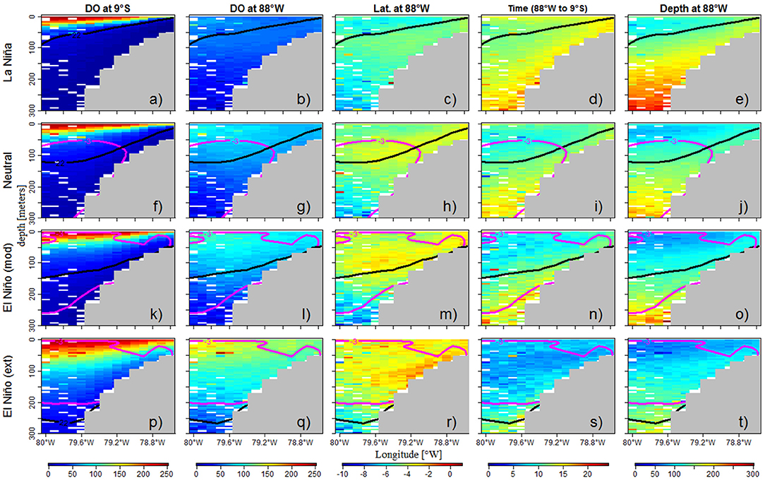
Figure 6. DO cross-shore section (9°S) during LN (a), Neutral (f), moderate (k) and extreme (p) EN. Equatorial (from 88°W) SW properties: DO concentration (b,g,l,q), latitude (c,h,m,r), travel time from 88°W to 9°S (d,i,n,s) and depth (e,j,o,t) during LN, Neutral, moderate and extreme EN periods. The properties were derived from floats released during spring of the ENSO phases. The PCUC (pink line) and ZO2 (black line) also are presented.

The changes in offshore oxygen content were related to changes in the location of the SW, associated with the modified SSCCs fluxes during ENSO. Within 100 km from the coast, during neutral periods, the SW originated from 3.5°S to 4°S (Figure 6h) and 110–140 m depth (Figure 6j). SW were then transported toward the coast for ~12 months (Figure 6i). During LN, SW were located south of 4.5°S (Figure 6c) and at greater depths (~160–180 m; Figure 6e), thus were less oxygenated (Figure 6b). Moreover, they were older since it took them more time (~15 months; Figure 6d) to reach the coastal section. In contrast, during EN, the SW were initially closer to the equator (3°S−1°S; Figures 6m,r), shallower (~100–120 m depth; Figures 6o,t) and thus more oxygenated (Figures 6l,q) than during LN and neutral periods. The SW transit time to the coastal region was much shorter (5–10 months; Figures 6n,s).

Eddy Oxygen Fluxes

As eddy activity is enhanced during ENSO (Chaigneau et al., 2008; Espinoza-Morriberón et al., 2017), we investigate the impact of EN and LN events on the oxygen vertical and horizontal fluxes.

The mean oxygen vertical flux ($\overline{\langle w\rangle .\langle O_2\rangle }$) presented positive values with a peak at ~40 m depth (Figure 7a). As the input of oxygen due to the mean flux is equal to—∂_z(〈w〉.〈O₂〉), it adds oxygen above ~40 m (mainly due to the decrease of mean vertical velocity near the surface, Figure 7d) and takes out oxygen in the subsurface layer between 40 and 150 m depth (due to the upwelling of less-oxygenated deep water from the OMZ core; e.g., Figures 3F–H). At the maximum flux depth (~40 m) the mean fluxes (~0.3 μmol m⁻² s⁻¹) did not present significant differences between neutral and LN periods (Wilcoxon test, p > 0.05), while a decrease was observed (~0.24 μmol m⁻² s⁻¹, ~20% reduction) during EN (Wilcoxon test, p < 0.05). This flux reduction was partly driven by the reduction of the vertical velocity (Figure 7d), which counteracted the impact of the subsurface oxygen increase (Figure 7c). Note that the modeled vertical velocity decrease (~40% at 50 m depth, Figure 7d) cannot be fully attributed to a decreased Ekman pumping during EN (e.g., Halpern, 2002; Chamorro et al., 2018, for the 1997–1998 EN), as it was only ~5% in our simulation (Figure not shown).

FIGURE 7

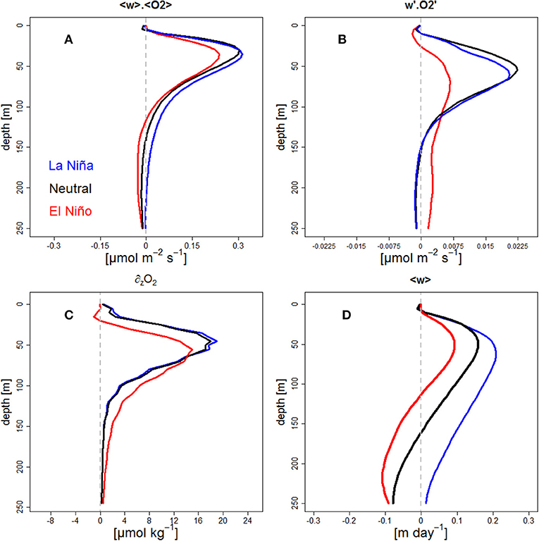
Figure 7. Vertical profile of DO mean vertical flux (A, in μmol O₂ m⁻² s⁻¹) and DO eddy vertical flux (B, in μmol O₂ m⁻² s⁻¹), DO vertical gradient (C, in μmol O₂ kg⁻¹ m⁻¹) and vertical velocity (D, in m day⁻¹) for Neutral (black line), LN (blue line), EN periods (red line). Profiles were computed in an oceanic band between 100 and 500 km from the coast and 6°S−14°S. In (C) dashed gray line represents the depth of the OMZ upper limit (22 μmol O₂ kg⁻¹).

The vertical eddy flux also presented positive values with a maximum at ~60 m depth (Figure 7b), which corresponds to the depth of maximum oxygen vertical gradient (∂_zO₂) (Figure 7c). In the stratified interior, mesoscale eddy fluxes tend to flatten the tilted upper thermocline (Colas et al., 2013) and hence the oxycline. Consequently, the vertical eddy flux brings oxygen into the layer above ~60 m, while below it acts as an oxygen sink and reinforces the OMZ. As for the mean flux, Neutral period presented a value of ~0.2 10⁻¹ μmol m⁻² s⁻¹ at 60 m, and was not significantly different to LN (Wilcoxon test, p > 0.05), while lower values (~0.06 10⁻¹ μmol m⁻² s⁻¹, ~70% decrease) and significant differences (Wilcoxon test, p < 0.05) were observed during EN between 50 and 70 m depth. This was associated to a reduction of the oxygen mean vertical gradient during EN (Figure 7c). As a consequence, the vertical gradient of the vertical eddy flux [-∂_z($w^{\prime }{O_2}^{\prime }$)] was also much weaker during EN than during LN and neutral periods. This highlights the much weaker role of the eddies as sink/source of oxygen below/above the oxycline during EN periods. At depths >100 m, the vertical eddy flux reached values close to zero during neutral and LN periods, whereas slightly positive values (~0.02 10⁻¹ μmol m⁻² s⁻¹) were found during EN.

Figure 8 shows the horizontal oxygen eddy fluxes at 100 and 400 m during ENSO phases and neutral periods. Intense eddy fluxes are found in the vicinity of the OMZ boundaries, mainly along the southern limit of the OMZ at 100 m depth and in the equatorial region (4°N−4°S) at 400 m depth. Hence this is logically the case at the lateral boundaries of the OMZ, especially at its southern limit where the horizontal gradient of DO is intense at 100 m depth. Eddy advection tends to inject oxygen into the OMZ, and it is more intense at shallower depths. During EN, at 100 m depth, the horizontal oxygen eddy fluxes increased (~+0.5 μmol m⁻² s⁻¹; Figure 8C) along the OMZ southern boundary and alongshore (~5°S−18° S) from the coast to 250 km offshore (Figure 8D). This indicates that eddy fluxes contributed to oxygenate the coastal region. At 400 m, fluxes were much weaker than at 100 m but also enhanced during EN periods (+~0.25 10⁻¹ μmol m⁻² s⁻¹; Figure 8G), both at the southern and mainly at the northern limits of the OMZ and along the northern shelf (Figure 8H). Eddy fluxes were quite similar during LN and neutral periods (Figures 8A,E). Overall, the OMZ ventilation at its lateral boundaries by mesoscale eddy advection increased during EN, whereas ventilation due to vertical eddy fluxes reduced.

FIGURE 8

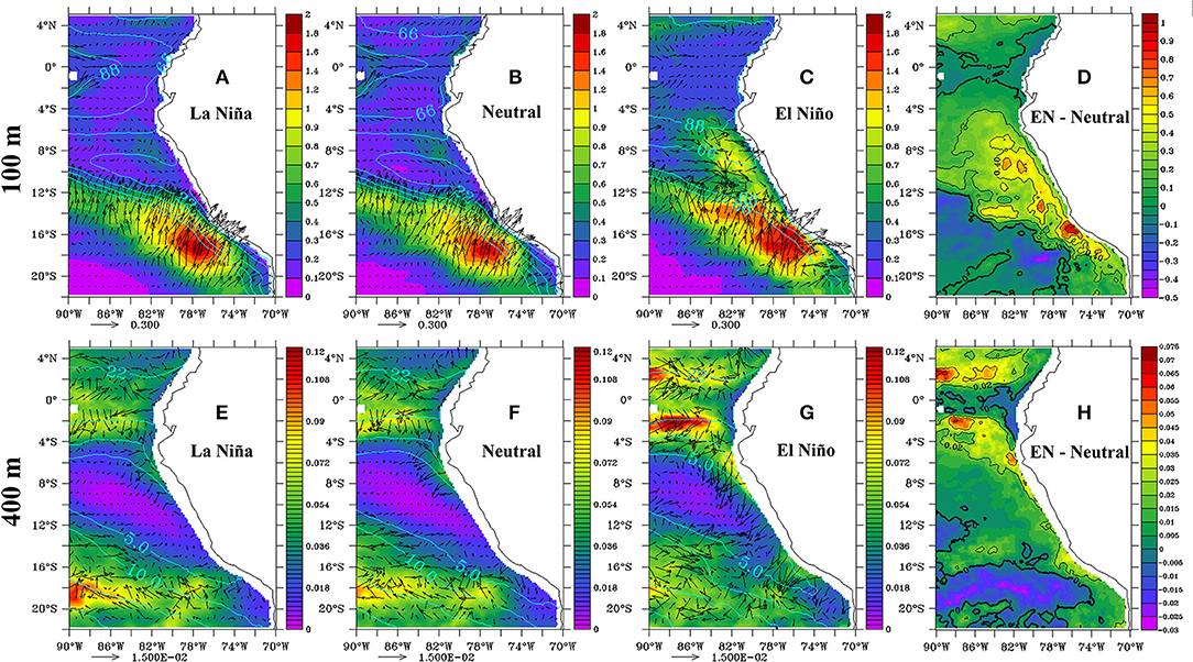
Figure 8. Intensity (colors, in μmol O₂ m⁻² s⁻¹) and direction (arrows) of the horizontal eddy fluxes ($\sqrt{{(u^{\prime }.O_2^{\prime })}^2+{(v^{\prime }.O_2^{\prime })}^2}$) at 100 m (top) and 400 m (bottom) averaged during LN (A,E), Neutral (B,F), and EN (C,G) events. The differences between EN and neutral period at 100 m (D) and 400 m (H) are also presented.

Biologeochemical Drivers of O₂ Changes During ENSO

The OMZ changes due to biogeochemical processes is investigated. The vertical profiles of biogeochemical source and sinks of oxygen (see Equation 2 in section The Oxygen Cycle in the PISCES Model) were averaged horizontally within 200 km to the coast (Figure 9). Most of the modeled biogeochemical processes related to the oxygen cycle take place in the near-surface layers and impact the OMZ indirectly through subduction of oxygen-enriched/depleted waters into the oxycline (e.g., Thomsen et al., 2016). The annual mean profiles of DO production and consumption had an exponential decrease with depth, with the exception of nitrification. The new and regenerated production (through photosynthesis) provided oxygen to the upper ocean above the ZO2 (~100 m depth). Remineralization was the main process consuming oxygen in surface and subsurface water, above 300 m. Microzooplankton respiration consumed oxygen above the upper limit of the OMZ, while mesozooplankton respiration was also found at depth. Oxygen consumption by nitrification peaked at 30 m in oxygen-repleted waters, as it is inhibited by light (Yoshioka and Saijo, 1984) near the surface (0–10 m depth). Nitrification decreased in the subsurface layer due to oxygen limitation (see Equation 2 in section The Oxygen Cycle in the PISCES Model). Within the OMZ (below 120 m depth), only oxygen consumption was observed (due to remineralization, mesozooplankton respiration, and nitrification).

FIGURE 9

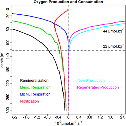
Figure 9. Mean vertical profiles of the DO biogeochemical sources and sinks (in 10⁻³ μmol O₂ m⁻³ s⁻¹): new (cyan line) and regenerated (magenta line) production, remineralization (black line), respiration by microzooplankton (blue line) and microzooplankton (green line), and nitrification (red line). The profiles were computed from 6°S to 16°S and with 200 km from the coast. Negative and positive values indicate DO consumption and production, respectively.

The impacts of EN and LN on the oxygen sources and sinks were diagnosed in the surface layer (above 100 m depth) and within ~60 km from the coast (Figure 10). Note that the sinks (i.e., negative terms in Equation 1, section The Oxygen Cycle in the PISCES Model) are shown here with a positive sign, meaning that positive (resp. negative) sink anomalies (e.g., Figures 10C–F, I–L) indicate an increase in oxygen consumption.

FIGURE 10

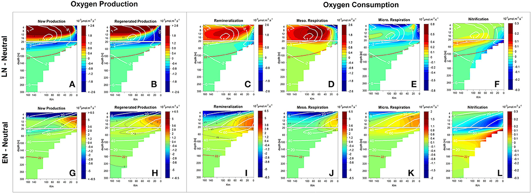
Figure 10. Alongshore-averaged vertical sections of DO anomaly sources (by new and regenerated production) (A,B,G,H) and sinks (remineralization, respiration by zooplankton and nitrification) (C–F,I–L) in 10⁻³ μmol O₂ m⁻³ s⁻¹ during LN (Top) and EN (Bottom) periods. The sign of the sink terms has been changed to positive in this figure. DO anomalies (white lines) and the isoline of 22 μmol O₂ kg⁻¹ (red lines) are presented.

During LN, a positive anomaly (>2 10⁻³ μmol m⁻³ s⁻¹) produced by the increase in new and regenerated production was found in a very thin surface layer (above ~10 m) and ~20 km offshore. In contrast, just below (10–80 m depth) and nearshore (within 20 km from the coast), new and regenerated production were weaker by ~-0.45 and ~-0.8 10⁻³ μmol m⁻³ s⁻¹, respectively, (Figures 10A,B).

During EN, the production of oxygen decreased (< -6.5 10⁻³ μmol m⁻³ s⁻¹), while new (~+0.46 10⁻³ μmol m⁻³ s⁻¹), and regenerated (~+0.73 10⁻³ μmol m⁻³ s⁻¹) productions were enhanced in the subsurface layer between 10 and 80 m depth nearshore and within 60 km from the coast (Figures 10G,H).

During ENSO phases, oxygen consumption was also strongly modified (Figures 10C–F,I–L) with anomalies of DOC remineralization and zooplankton respiration presenting marked cross-shore patterns. Nearshore, negative and positive anomalies predominated during LN and EN, respectively, while ~30 km offshore and above 15 m, opposite sign patterns were found. Nitrification anomalies presented a pronounced vertical gradient. Below ~30 m depth, the nitrification decreased and increased during LN and EN, respectively, due to the presence/absence of oxygen.

During LN, remineralization, mesozooplankton, and microzooplanton respiration within ~20 km from the coast were characterized by negative anomalies of −0.29, −0.28, and −0.16 10⁻³ μmol m⁻³ s⁻¹, respectively, (Figures 10C–E), likely due to the stronger offshore advection of properties. A deficit of nitrification (−0.13 10⁻³ μmol m⁻³ s⁻¹) was found above the shelf (20–60 m; Figure 10F).

In contrast, remineralization decreased in a thin surface layer (0 – ~10 m) but strongly increased below, down to 100 m depth during EN. Positive anomalies of +1.6 10⁻³ μmol m⁻³ s⁻¹ were found nearshore (within ~80 km from the coast and between 10 and 80 m, Figure 10I). Expectedly, meso and microzooplankton respiration reduced in a thin surface layer and increased at depth above the shelf, producing positive anomalies of +0.55 and +0.31 10⁻³ μmol m⁻³ s⁻¹, respectively, between 10 and 80 m and from 0 to 80 km to the coast (Figures 10J,K). Last, nitrification was less intense between the surface and 40 m depth and increased near the bottom over the shelf (+0.21 10⁻³ μmol m⁻³ s⁻¹ between 40–100 m and 0–80 km from the coast; Figure 10L). Nitrification, which was switched off in this depth range during neutral and LN conditions due to the lack of oxygen, took place during EN as shelf waters became oxygenated.

Impact of the Remote and Local Forcing During ENSO

Sensitivity experiments (see section Model Experiments and Table 1) were performed to investigate the impact of remote (Kclim) and local forcing (Wclim) on the OMZ during ENSO. Figure 11 shows the oxygen changes (in %), in Kclim and Wclim with respect to CR, in an alongshore- averaged (between 6°S and 16°S) cross-shore section (see also Figure 3).

FIGURE 11

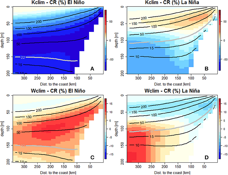
Figure 11. Alongshore-averaged vertical sections of DO concentration change (in %) for Kclim (A,C) and Wclim (B,D) with respect to CR, during LN (top) and EN (bottom). Black isolines mark DO concentration during LN (A,B) and EN (C,D) in the CR simulation. Note the different scale for Kclim and Wclim due to the stronger DO changes in Kclim.

During LN, the oxygen content increased slightly (~10%, +10 μmol kg⁻¹) in Kclim with respect to CR in the surface layer (between 0 and 50 m depth and within 200 km from the coast, Figure 11A). In this experiment, the ZO2 shoaling forced by the LN upwelling CTW was absent.

In contrast, a moderate DO decrease (10–20%, −2 μmol kg⁻¹) was found below the upper limit of the OMZ. When the interannual wind variability is suppressed (Wclim), a moderate oxygen decrease (~3%, ~-8 μmol kg⁻¹) was found above the ZO2 (Figure 11B). Below the ZO2, the DO concentration increased offshore by 10% (~+2 μmol kg⁻¹).

During EN, a strong DO reduction was found over the entire water column in Kclim. It was strongest between 90 and 150 m depth, where DO was ~60 % (~-55 μmol kg⁻¹) lower than in CR (Figure 11C). In contrast, more oxygen was found (12%, +10 μmol kg⁻¹) in Wclim than in CR between 40–130 m depth and 50–250 km offshore (Figure 11D).

Discussion

Bias of the Modeled OMZ

The interannual variability of the main physical parameters, surface productivity and nutrients simulated by our model were validated in Espinoza-Morriberón et al. (2017). The model reproduced well the changes of SSH, temperature, nutrients and chlorophyll-a (Chl) in surface and subsurface waters during both EN and LN phases. Here, we show that the model reproduced deoxygenation and oxygenation during LN and EN, respectively, in agreement with previous studies based on in situ data analysis (Graco et al., 2007, 2017; Gutiérrez et al., 2008). In addition, in annual mean, the shoaling of ZO2 toward the coast (~50 m depth) was also observed between 14°S and 16°S by Graco et al. (2007), likely associated with coastal upwelling. Nevertheless, some discrepancies were observed. First, between 2°N and 2°S, observational data evidenced a thin and coastal OMZ (e.g., Karstensen et al., 2008; Czeschel et al., 2015; Llanillo et al., 2018), that is not reproduced by our simulation. This may be due to the intense EUC simulated by the SODA model (used as the physical OBC forcing in our simulation) which ventilates the equatorial region (Montes et al., 2014). Off Peru, overly low DO (<5 μmol kg⁻¹) was found within the modeled OMZ core (Figures 2, 3) in line with Karstensen et al. (2008). However, this bias with respect to the CARS climatology and IMARPE observations could be partly due to the numerical artifacts during the construction of the 3D fields and/or to the inclusion of records from old instruments which were not sufficiently accurate at low DO values (Bianchi et al., 2012). Underestimation of OMZ volumes slightly more oxygenated than the core was also reported i.e., Fuenzalida et al. (2009). Blending vertical high-resolution CTDO profiles with quality-controlled bottle casts from WOD01, Fuenzalida et al. (2009) found that the extent of hypoxic areas (<60 μmol kg⁻¹) in the TSEP was underestimated in global databases such as WOA01. Note that the more recent WOA 2013 DO climatology (Garcia et al., 2013) did not display lower values than CARS (Figure not shown), so for that reason we chose the latter.

Crude parameterization of the oxygen cycle in the PISCES model, due to the fixed-in-time values of biogeochemical parameters (e.g., remineralization rate of DOC and nitrification rate) throughout the interannual simulation may also impact the modeled OMZ. For example, the remineralization rate of DOC only takes into account a proxy of bacterial concentration and DOC concentration in PISCES (Aumont et al., 2015), even though temperature changes (which are particularly strong during EN) impact the bacterial metabolic rates involved in the oxygen cycle (López-Urrutia et al., 2006), an effect seldom included in biogeochemical models (Segschneider and Bendtsen, 2013). Note also that previous regional models of the OMZ using the nitrogen-based BioEBUS model (Gutknecht et al., 2013) also produced a more intense OMZ than the observations (Montes et al., 2014; Vergara et al., 2016; Mogollón and Calil, 2017).

Last, we cannot exclude the possibility that our boundary forcing (SODA) may have partly induced the very low OMZ concentrations simulated by our model. Indeed, Montes et al. (2014) showed that using different sets of physical OBCs, which differed in the SSCCs vertical structure intensity, could modify the shape and intensity of the OMZ.

Impact of Eastward Fluxes From the Equatorial Region

The equatorial circulation was impacted during ENSO, which modified the eastward oxygen fluxes in the equatorial region offshore of the PCUS. To illustrate it, the intensity of the zonal currents (EUC, pSSCC, and sSSCC) and associated oxygen fluxes at 88°W between 50 and 200 m were computed (Table 2). The EUC was weaker during EN and LN than during neutral conditions. Stramma et al. (2016) also found a strong weakening of the EUC velocity during the onset (October) of the 2015–2016 EN. In contrast, the SSCCs intensity increased during EN with respect to LN and neutral conditions. These results are in line with Montes et al. (2011), who simulated the circulation during the moderate 2002–2003 EN and 1999–2000 LN. Even though stronger SSCCs were observed during EN, the nearshore water column (e.g., at 9°S, Figure 6) was mainly fed by waters initially transported by the EUC. The water masses transit time from 88°W to the nearshore region ranged from ~15 months during LN to ~6 months during EN (Espinoza-Morriberón et al., 2017). During LN, the longer transit may partly explain the nearshore oxygen deficit due to microbial respiration in the transported water mass. Furthermore, note that the fast pathway observed in the model during EN, from the equatorial regions to the coastal range, was also found by Montes et al. (2011) for the 2002–2003 EN (~2–4 months). This shows that not all particles released in the equatorial zone reached the nearshore regions during the same ENSO phase. In the equatorial region, in our simulation, the oxygen fluxes variability is driven by the equatorial currents variability, and not by oxygen variability as oxygen western boundary conditions are climatological. Thus, the oxygen fluxes from the SSCCs and the EUC were less intense during LN than during EN (an exception is the EUC flux during moderate EN; see Table 2). During EN, enhanced SSCCs oxygen contributed to reduce the OMZ volume and displace its offshore boundaries eastward (Montes et al., 2014).

TABLE 2

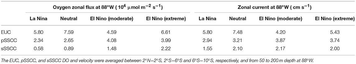
Table 2. DO mean zonal fluxes (in 10⁴ μmol m⁻² s⁻¹) and intensity of the zonal currents (in cm s⁻¹) from the EUC, pSSCC, and sSSCC during LN, Neutral and, moderate and extreme EN periods.

Ventilation by Eddy Fluxes

The horizontal eddy fluxes play an important role in structuring the OMZ lateral extent (Vergara et al., 2016) where strong oxygen horizontal gradients are found. It is well-known that eddy tracer fluxes are downgradient (and pronounced) when there is a strong sink in the tracer distribution (e.g., Wilson and Williams, 2006). In a recent modeling study, Vergara et al. (2016), showed that horizontal eddy fluxes through the OMZ coastal boundary attains its maximum in winter in association with a maximum seasonal Eddy Kinetic Energy (EKE). Similarly, the EKE increase during EN induces a large interannual horizontal eddy flux which ventilates the nearshore OMZ. The magnitude of this enhanced interannual ventilation by horizontal eddy fluxes could be underestimated due to the relatively low horizontal resolution (1/6°) of our model (e.g., Capet et al., 2008; Colas et al., 2013). However, a resolution of 1/6° is considered eddy-resolving off Peru: due to its proximity to the equator, the typical length scale of mesoscale structures would be covered by ~10 grid points (Belmadani et al., 2012). Indeed, in spite of this caveat, our model represented correctly the spatial and interannual variability of the EKE (Espinoza-Morriberón et al., 2017). Nevertheless, a more complete modeling study with an increased spatial resolution would be needed to better understand and quantify the role of submesoscale variability on the OMZ (Thomsen et al., 2016).

Biological Processes

Remineralization is the major oxygen sink in the water column (Paulmier and Ruiz-Pino, 2009) and is mainly produced by bacterial respiration off Peru (Kalvelage et al., 2015). This is reproduced in our modeling results (Figure 9). Furthermore, zooplankton respiration has been little studied in the PCUS in spite of its high oxygen demand in the water column. Global estimates of mesozooplankton respiration (in fraction of body carbon respired daily) indicated that it represents ~17–32% of the photosynthetic carbon produced in the open ocean (underestimated in previous works e.g., del Giorgio and Duarte, 2002; Hernández-León and Ikeda, 2005). In our configuration, the zooplankton respiration represented ~33% of the oxygen produced by photosynthesis (between 6°S−16°S and 0–200 m depth), close to global estimates. High biomass of zooplankton has been found in the PCUS, showing that zooplankton can adapt to low-oxygen conditions at great depths (Ayón et al., 2008; Ballón et al., 2011). This implies a high oxygen consumption at greater depths due to the mesozooplankton respiration, which is more tolerant to suboxic condition than microzooplankton (this is explicitly included in PISCES). However, due to a lack of data, the zooplankton biomass in PISCES (see Figure 14 in Espinoza-Morriberón et al., 2017) could not be evaluated, which is needed to estimate reliable respiration rates.

Our model setting has also some limitations, as the nitrogen cycle is crudely parameterized in PISCES (Aumont et al., 2015). High concentrations of nitrous oxide (N₂O), a potent greenhouse gas produced during nitrification (Codispoti and Christensen, 1985), have been observed off the Peruvian coasts (Kock et al., 2016), especially during pulses of oxygenation. Although not simulated by our model, production of nitrous oxide is likely to occur during EN due to enhanced nitrification in subsurface layers (Figure 10L). Using the nitrogen-cycle-based ROMS-BioEBUS coupled model, Mogollón and Calil (2017) found a decrease (80 %) of nitrification between the peaks of 1997–1998 EN and 1999–2000 LN and production of nitrous oxide during EN. In line with this study, our model simulated a nearshore nitrification decrease of ~60% between EN and LN (within 20 km from the coast and between 20 and 80 m depth). Furthermore, under suboxic conditions (<5–10 μmol kg⁻¹), both anammox (Lam et al., 2009), and denitrification could produce N loss (Dalsgaard et al., 2012). The percentage of N loss contribution by both processes depends on ENSO phases. During 1997–1998 EN, anammox, and denitrification contribute to N loss of 40 and 60%, respectively, while during 1999–2000 LN the contribution of anammox increase of 70% (Mogollón and Calil, 2017). In PISCES, anammox is not included, which could explain the overestimation of nitrate in our simulation (see Figure 3 in Espinoza-Morriberón et al., 2017).

In PISCES, denitrification occurred in regions of DO <6 μmol kg⁻¹ (hereafter ODZ) and was simply parameterized using DOC and a remineralization rate (Aumont et al., 2015):

$\begin{array}{l}Denit=R_{NO3}*{\lambda }_{DOC}^{*}*(△O_2)*DOC\end{array}$

Where R_NO3 represents the N/C stoichiometric ratio. Our model simulated an increase of the denitrification in nearshore and shallower waters during LN (e.g., during the 1999–2000 LN, Figure 12a), due to the shoaling of the ODZ, despite of the unchanged ODZ volume. This is likely due to a shoaling of the OMZ (Figure 3J), which allowed denitrification to occur at shallower depths, and enhanced remineralization (Figure 10C). In contrast, during EN, the ventilated water column inhibited denitrification above ~200 m, and a deeper offshore ODZ was observed (e.g., during the 1997–1998 EN, Figure 12b). Overall, denitrification within the ODZ (defined between 6°S−16°S, 0–500 km, and 0–500 m depth) increased by ~25% during LN and decreased by ~60% during EN (moderate or extreme), with respect to neutral periods (Figure 12c). Using a global biogeochemical model, Yang et al. (2017) found a denitrification increase of ~70% between the peak of 1997–1998 EN and 1999–2000 LN, which is close to our estimate (~85%).

FIGURE 12

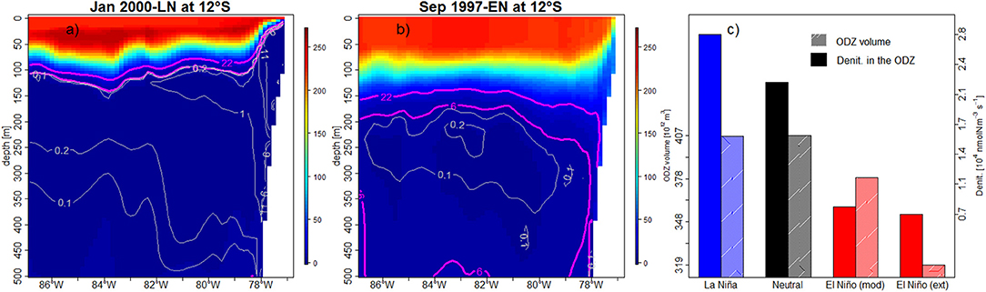
Figure 12. Cross-shore vertical sections (12°S) of DO concentration (color shading and magenta lines, in μmol O₂ kg⁻¹) and denitrification (gray lines, in 10⁴ nmolN m⁻³ s⁻¹) during the peak of 1997–1998 EN (a) and 1999–2000 LN (b) at 12°S. (c) WDC volume and mean denitrification during LN (blue bar), Neutral (black bar), moderate and extreme EN (red bars).

On the other hand, DO changes during LN and EN were influenced not only by physical processes but also by changes in DO production related to primary productivity changes above the upper limit of the OMZ, between 0 and ~20 m. The nearshore DO changes induced an increased (decrease) oxygen consumption by remineralization and respiration during EN (LN). During LN, more (less) oxygen production was found at surface (sub-), due to the thinner mixed layer during LN, in which primary production was confined (Espinoza-Morriberón et al., 2017). In contrast, during EN, the nutricline depth increased and photosynthesis decreased in the surface layer (Espinoza-Morriberón et al., 2017), producing less oxygen.

Oxygen consumption decreased and increased during LN and EN, respectively (mainly at subsurface), due to DO availability. The relationship between the oxygen consumption and DO availability was also evidenced offshore (86°W) using in situ data during the 2009 LN (Llanillo et al., 2013). The authors found an increase of the oxygen consumption by respiration and remineralization within the OMZ due to the presence of the oxygen-rich Antarctic Intermediate Waters (AAIW).

Remote and Local Drivers of DO Interannual Variability

The equatorial remote forcing was the main driver of changes in the ZO2 and OMZ core during both EN and LN. The passage of downwelling and upwelling CTWs trigger the oxygenation (in the surface and subsurface layers) and deoxygenation (only in the surface layer) during EN and LN, respectively. At subsurface during LN, remotely-forced deep coastal waves (e.g., Pietri et al., 2014) may enhance the equatorward transport of the oxygenated AAIW, which ventilates the deep OMZ between ~150–350 m and 6°S−14°S (e.g., LN 2009; Llanillo et al., 2013).

The strong relationship between the variability of ZT15 and ZO2 is well known locally at specific coastal sites off Peru (e.g., 12°S, Gutiérrez et al., 2008; Graco et al., 2017), and in other regions where CTWs play an important role, e.g., Vallivattathillam et al. (2017) for the western coast of India. These authors mentioned that the effects of biogeochemical processes (e.g., remineralization and respiration) and of vertical mixing were smaller than those due to advection (e.g., CTW). This strong relationship is highlighted in Figure 13A, which shows the spatial pattern of correlation between ZT15 and ZO2 monthly anomalies over the entire PCUS. The correlation was highest (~0.8) nearshore (between the coast and 50 km offshore) and dropped offshore and south of 18°S, where the OMZ vanishes. The high correlation pattern extended westward until 350 km offshore along 10°S. North of 10°S, the correlation decreased due to a ZO2 deepening larger than that of ZT15. Figures 13B–C show cross-shore sections of the correlation between ZO2 and ZT15 and the depth difference at 7°S and further south, at 10°S. At 7°S (Figure 13B), the OMZ was more impacted by ENSO (Mogollón and Calil, 2017) and by the eastward SSCCs transporting oxygen-rich waters (Montes et al., 2014), leading to the increasing distance between ZO2 and ZT15 and correlation decrease west of 81°W. The ZO2 was shallower at 10°S than at lower latitudes (Figures 2b,c) as it was less impacted by the oxygen-rich waters transported eastward by the EUC and SSCCs. Note that the correlation was very high along the coasts of Colombia and Central America. This indicates that the nearshore interannual variability of ZO2 in the northern hemisphere is also controlled by the shoaling and deepening of isotherms during the poleward propagation of CTWs.

FIGURE 13

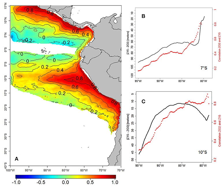
Figure 13. Spatial correlation between modeled ZT15 and ZO2 monthly anomalies in the period 1958–2008 (A). Mean absolute difference (|ZT15–ZO2|, black line, in meters) and correlation (red line) between ZO2 and Z15, from the coast to 95°W, at 7°S (B) and 10°S (C).

On the other hand, local wind fluctuations played a minor role in oxygenation/deoxygenation processes at interannual time scales. During EN, when the interannual wind variability is suppressed (in Wclim), a relatively weak subsurface oxygen increase is observed. This can be explained as follows: as the alongshore wind increases during EN (see Figure 9 in Enfield, 1981; Espinoza-Morriberón et al., 2017; Chamorro et al., 2018), the coastal upwelling intensifies. This partly compensates the ZO2 deepening, bringing deep oxygen-poor waters in this depth range. As the EN enhanced wind-driven upwelling was absent in Wclim, the ZO2 was deeper and DO higher than in the CR. During LN, an oxygen decrease was observed above 50 m, in the absence of interannual wind variability (Wclim). Primary production was reduced with respect to CR (between ~4 and 40 m), thus less oxygen was produced by photosynthesis above 30 m within 200 km to the coast (figure not shown). However, the DO increase offshore and below the ZO2 is possibly related to a reduction (~20%) of the (positive) Ekman pumping during LN in Wclim, which results in less upward transport of oxygen-poor waters than in CR.

Impact of ENSO Diversity

It is important to mention that our analysis did not take into account the diversity of EN events. Indeed, a Central-Pacific (CP) EN (Modoki; e.g., Takahashi et al., 2011) is likely to impact the OMZ differently than a canonical Eastern Pacific (EP) EN. CP EN events are frequently associated to upwelling CTWs during fall and winter, in contrast with the more frequent downwelling CTWs observed during EP EN (Dewitte et al., 2012). Thus, during EN Modoki poor oxygen waters could be more present than during a canonical EN, due to a shoaling of the ZO2 triggered by the passage of the upwelling CTWs (e.g., Figure 5f). Besides, in early 2017 a “coastal El Niño” occurred (Takahashi and Martínez, 2017; Garreaud, 2018), which also had a different impact on the DO. In fact, during canonical EN (e.g., 2015–2016 EN) a deepening of the ZO2 occurred, while during the summer of 2017 (Coastal EN) the impact was greater in the surface layer but the ZO2 stayed shallower (ENFEN, 2017).

Conclusions and Perspectives

In the present work, the physical and biological processes that drive the interannual variability of the TSEP OMZ were studied using the physical-biogeochemical ROMS-PISCES coupled model. First, an evaluation of our interannual simulation over the period 1958–2008 showed that, despite a reasonable bias in the representation of the modeled OMZ, the phases of oxygenation and deoxygenation during EN and LN were qualitatively well reproduced. During EN, the nearshore ZO2 deepened due to the passing of remotely-forced intense “downwelling” CTWs. During LN, the ZO2 shoaled due to the less intense “upwelling” CTWs, enabling oxygen-depleted waters to accumulate on the shelf. The remote equatorial forcing (IEKWs) was responsible for the tight correlation between the thermocline and ZO2 close to the coasts.

Furthermore, the characteristics of the equatorial SW which were transported toward the coast and fueled the nearshore water column were investigated. SW were mainly transported eastward by the SSCCs (located south of the equator) and EUC during LN and EN, respectively, before reaching the Peru coast. During EN the SW were more oxygenated as they originated from the north of the OMZ and transited faster to the coastal region than during LN.

The vertical and horizontal oxygen eddy fluxes were also evaluated. On average, the offshore (between 100 and 500 km from the coast and 6°S−14°S) vertical eddy flux brings oxygen to the surface layer (above ~60 m), while it removed oxygen below. This flux was not modified during LN, but during EN a very strong decrease was observed, due to the reduced oxygen vertical gradient resulting from the deepening of the ZO2. Horizontal eddy fluxes tended to inject oxygen into the OMZ from its lateral boundaries, especially at its southern limit where the horizontal gradient of O₂ is intense. This was not modified during LN with respect to neutral period. However, during EN, the horizontal oxygen eddy fluxes strongly increased due to the increase of eddy activity, intensifying eddy-driven horizontal ventilation.

Regarding the biogeochemical processes, remineralization was the main process consuming oxygen in the water column, followed by zooplankton respiration and nitrification. These oxygen sinks were strongly altered during ENSO phases, depending on oxygen availability in the water column.

Sensitivity experiments performed to evaluate the influence of the equatorial remote (i.e., CTWs) and local forcing (e.g., wind), demonstrated that the equatorial forcing had a greater impact than local winds on the DO changes, in particular during EN.

Future studies will address the mechanisms which drive the DO changes off Peru over the last decades. While a deoxygenation trend has been observed in the open ocean (Stramma et al., 2008; Breitburg et al., 2018), a nearshore shoaling of the TSEP OMZ has also been described in the late 2000s (Bertrand et al., 2011). In contrast, a relative oxygenated-water column was observed in the last decade on the Peru central shelf, likely due to more frequent downwelling CTW (Graco et al., 2017). Future studies will also address the impact of climate change in the PCUS. As downscaled projections of climate scenarios in the PCUS simulated a strong near-surface stratification increase (Echevin et al., 2011; Oerder et al., 2015), this could hamper ventilation and intensify the OMZ. However, further deep and poleward proxy data and instrumental observations suggest ventilation of the OMZ core over the last decades (Cardich et al., in review).

Author Contributions

DE-M proposed the original idea of the study, produced most of the material and wrote the manuscript. VE, FC, DG, JT, MG, and CQ-C discussed the results and corrected the manuscript. JL participated to the in situ data collection.

Conflict of Interest Statement

The authors declare that the research was conducted in the absence of any commercial or financial relationships that could be construed as a potential conflict of interest.

The handling editor is currently editing co-organizing a Research Topic with one of the authors (DG), and confirms the absence of any other collaboration.

Acknowledgments

DE-M was supported by an individual doctoral research grant from the Allocations de Recherche pour une Thèse au Sud (ARTS) IRD program. DE-M also acknowledges CIENCIACTIVA/CONCYTEC-PERU for financial support during training periods at LOCEAN (Sorbonne Université). Numerical simulations were performed on the ADA computer at IDRIS (project i2015011140). The model results are available upon request to despinoza@imarpe.gob.pe and vincent.echevin@locean-ipsl.upmc.fr. This work is a contribution from the Cooperation agreement between the IMARPE and the Institut de Recherche pour le Développement (IRD), through the LMI DISCOH.

Supplementary Material

The Supplementary Material for this article can be found online at: https://www.frontiersin.org/articles/10.3389/fmars.2018.00526/full#supplementary-material

References

Albert, A., Echevin, V., Lévy, M., and Aumont, O. (2010). Impact of nearshore wind stress curl on coastal circulation and primary productivity in the Peru upwelling system. J. Geophys. Res. 115:C12033. doi: 10.1029/2010JC006569

CrossRef Full Text | Google Scholar

Aumont, O., Ethé, C., Tagliabue, A., Bopp, L., and Gehlen, M. (2015). PISCES-v2: an ocean biogeochemical model for carbon and ecosystem studies. Geosci. Model. Dev. 8, 2465–2513. doi: 10.5194/gmd-8-2465-2015

CrossRef Full Text | Google Scholar

Ayón, P., Criales-Hernandez, M. I., Schwamborn, R., and Hirche, H.-J. (2008). Zooplankton research off Peru: a review. Prog. Oceanogr. 79, 238–255. doi: 10.1016/j.pocean.2008.10.020

CrossRef Full Text | Google Scholar

Babbin, A. R., Keil, R. G., Devol, A. H., and Ward, B. B. (2014). Organic matter stoichiometry, flux, and oxygen control nitrogen loss in the ocean. Science 344, 406–408. doi: 10.1126/science.1248364

PubMed Abstract | CrossRef Full Text | Google Scholar

Ballón, M., Bertrand, A., Lebourges-Dhaussy, A., Gutiérrez, M., Ayón, P., Grados, D., et al. (2011). Is there enough zooplankton to feed forage fish populations off Peru? An acoustic (positive) answer. Prog. Oceanogr. 91, 360–381. doi: 10.1016/j.pocean.2011.03.001

CrossRef Full Text | Google Scholar

Belmadani, A., Echevin, V., Dewitte, B., and Colas, F. (2012). Equatorially forced intraseasonal propagations along the Peru–Chile coast and their relation with the nearshore eddy activity in 1992–2000: a modeling study. J. Geophys. Res. 117:C04025. doi: 10.1029/2011JC007848

CrossRef Full Text | Google Scholar

Bertrand, A., Chaigneau, A., Peraltilla, S., Ledesma, J., Graco, M., Monetti, F., et al. (2011). Oxygen: a fundamental property regulating pelagic ecosystem structure in the Coastal Southeastern Tropical Pacific. PLoS ONE 6:e29558. doi: 10.1371/journal.pone.0029558

PubMed Abstract | CrossRef Full Text | Google Scholar

Bianchi, D., Dunne, J. P., Sarmiento, J. L., and Galbraith, E. D. (2012). Data-based estimates of suboxia, denitrification, and N2O production in the ocean and their sensitivities to dissolved O₂. Global Biogeochem. Cy. 26:GB2009. doi: 10.1029/2011GB004209

CrossRef Full Text | Google Scholar

Breitburg, D., Levin, L. A., Oschlies, A., Grégoire, M., Chavez, F. P., Conley, D. J., et al. (2018). Declining oxygen in the global ocean and coastal waters. Science 359:eaam7240. doi: 10.1126/science.aam7240

PubMed Abstract | CrossRef Full Text | Google Scholar

Capet, X., McWilliams, J. C., Molemaker, M. J., and Shchepetkin, A. F. (2008). Mesoscale to submesoscale transition in the California current system. Part I: flow structure, eddy flux, and observational tests. J. Phys. Oceanogr. 38, 29–43. doi: 10.1175/2007JPO3671.1

CrossRef Full Text | Google Scholar

Capet, X. J., Marchesiello, P., and McWilliams, J. C. (2004). Upwelling response to coastal wind profiles. Geophys. Res. Lett. 31:L13311. doi: 10.1029/2004GL020123

CrossRef Full Text | Google Scholar

Carrit, D. E., and Carpenter, J. H. (1966). Recommendation procedure for Winkler analyses of seawater for dissolved oxygen. J. Mar. Res. 24, 313–318.

Google Scholar

Carton, J. A., and Giese, B. (2008). A reanalysis of ocean climate using Simple Ocean Data Assimilation (SODA). Mon. Weather Rev. 136, 2999–3017. doi: 10.1175/2007MWR1978.1

CrossRef Full Text | Google Scholar

Cavan, E. L., Trimmer, M., Shelley, F., and Sanders, R. (2017). Remineralization of particulate organic carbon in an ocean oxygen minimum zone. Nat. Commun. 8:14847. doi: 10.1038/ncomms14847

PubMed Abstract | CrossRef Full Text | Google Scholar

Chaigneau, A., Dominguez, N., Eldin, G., Vasquez, L., Flores, R., Grados, C., et al. (2013), Near-coastal circulation in the Northern Humboldt Current System from shipboard ADCP data. J. Geophys. Res. Oceans. 118, 5251–5266. doi: 10.1002/jgrc.20328

CrossRef Full Text | Google Scholar

Chaigneau, A., Gizolme, G. A., and Grados, C. (2008). Mesoscale eddies off Peru in altimeter records: identification algorithms and eddy spatio-temporal patterns. Prog. Oceanogr. 79, 106–119. doi: 10.1016/j.pocean.2008.10.013

CrossRef Full Text | Google Scholar

Chamorro, A., Echevin, V., Colas, F., Oerder, V., Tam, J., and Quispe-Ccalluari, C. (2018). Mechanisms of the intensification of the upwelling-favorable winds during El Niño 1997–1998 in the Peruvian upwelling system. Clim Dynam. 51, 3717–3733. doi: 10.1007/s00382-018-4106-6

CrossRef Full Text | Google Scholar

Codispoti, L. A., Barber, R. T., and Friederich, G. E. (1989). “Do nitrogen transformations in the poleward undercurrent off Peru and Chile have a globally significant influence?,” in Poleward Flows Along Eastern Ocean Boundaries. Coastal and Estuarine Studies, eds S. J. Neshyba, N. K. Mooers, R. L. Smith, and R. Barber (Springer-Verlag New York, Inc.), 281–310. doi: 10.1029/CE034p0281

CrossRef Full Text | Google Scholar

Codispoti, L. A., and Christensen, J. P. (1985). Nitrification, denitrification and nitrous oxide cycling in the eastern tropical South Pacific Ocean. Mar. Chem. 16, 277–300. doi: 10.1016/0304-4203(85)90051-9

CrossRef Full Text | Google Scholar

Colas, F., Capet, X., McWilliams, J. C., and Li, Z. (2013). Mesoscale eddy buoyancy flux and eddy-induced circulation in Eastern Boundary Currents. J. Phys. Oceanogr. 43, 1073–1095. doi: 10.1175/JPO-D-11-0241.1

CrossRef Full Text | Google Scholar

Colas, F., McWilliams, J. C., Capet, X., and Kurian, J. (2012). Heat balance and eddies in the Peru-Chile current system. Clim Dynam. 39, 509–529. doi: 10.1007/s00382-011-1170-6

CrossRef Full Text | Google Scholar

Conkright, M., Locarnini, R., Garcia, H., O'Brien, T. D., Boyer, T. P., Stephens, C., et al. (2002). World Ocean Atlas 2001: Objectives, Analyses, Data Statistics and Figures, CD-ROM Documentation. NOAA Atlas NESDIS 42. Silver Spring, MD.

Czeschel, R., Stramma, L., Schwarzkopf, F. U., Giese, B. S., Funk, A., and Karstensen, J. (2011). Middepth circulation of the eastern tropical South Pacific and its link to the oxygen minimum zone. J. Geophys. Res. 116:C01015. doi: 10.1029/2010JC006565

CrossRef Full Text | Google Scholar

Czeschel, R., Stramma, L., Weller, R. A., and Fischer, T. (2015). Circulation, eddies, oxygen, and nutrient changes in the Eastern Tropical South Pacific Ocean. Ocean Sci. 11, 455–470. doi: 10.5194/os-11-455-2015

CrossRef Full Text | Google Scholar

Da Silva, A. M., Young, C. C., and Levitus, S. (1994). Atlas of Surface Marina Data 1994, Technical Report. National Oceanic and Atmospheric Administration, Silver Spring MD.

Dalsgaard, T., Thamdrup, B., Farías, L., and Revsbech, N. P. (2012). Anammox and denitrification in the oxygen minimum zone of the eastern South Pacific. Limnol. Oceanogr. 57, 1331–1346. doi: 10.4319/lo.2012.57.5.1331

CrossRef Full Text | Google Scholar

del Giorgio, P. A., and Duarte, C. M. (2002). Total respiration and the organic carbon balance of the open ocean. Nature 420, 379–384. doi: 10.1038/nature01165

CrossRef Full Text

Devol, A. H., Uhlenhopp, A. G., Naqvi, S. W. A., Brandes, J. A., Jayakumar, D. A., Naik, H., et al. (2006). Denitrification rates and excess nitrogen gas concentrations in the Arabian Sea oxygen deficient zone. Deep-Sea Res. 53, 1533–1547. doi: 10.1016/j.dsr.2006.07.005

CrossRef Full Text | Google Scholar

Dewitte, B., Vazquez-Cuervo, J., Goubanova, K., Illig, S., Takahashi, K., and Cambon, G., et al. (2012). Change in El Niño flavours over 1958–2008: Implications for the long-term trend of the upwelling off Peru. Deep Sea Res. Part 2, 77–80, 143–156. doi: 10.1016/j.dsr2.2012.04.011

CrossRef Full Text

Diaz, R. J., and Rosenberg, R. (2008). Spreading dead zones and consequences for marine ecosystems. Science 321, 926–929. doi: 10.1126/science.1156401

PubMed Abstract | CrossRef Full Text | Google Scholar

Echevin, V., Albert, A., Lévy, M., Aumont, O., Graco, M., and Garric, G. (2014). Remotely-forced intraseasonal variability of the Northern Humboldt Current System surface chlorophyll using a coupled physical-ecosystem model. Cont. Shelf. Res. 73, 14–30. doi: 10.1016/j.csr.2013.11.015

CrossRef Full Text | Google Scholar

Echevin, V., Aumont, O., Ledesma, J., and Flores, G. (2008). The seasonal cycle of surface chlorophyll in the Peruvian upwelling system: a model study. Prog. Oceanogr. 79, 167–176. doi: 10.1016/j.pocean.2008.10.026

CrossRef Full Text | Google Scholar

Echevin, V., Colas, F., Chaigneau, A., and Penven, P. (2011). Sensitivity of the Northern Humboldt Current System nearshore modeled circulation to initial and boundary conditions. J. Geophys. Res. 116:C07002. doi: 10.1029/2010JC006684

CrossRef Full Text | Google Scholar

ENFEN (2017), Technical Report ENFEN. Available online at: https://www.dhn.mil.pe/Archivos/oceanografia/enfen/informe-tecnico/03-2017.pdf

PubMed Abstract

Enfield, D. B. (1981). Thermally driven wind variability in the planetary boundary layer above Lima, Peru. J. Geophys. Res. 86, 2005–2016. doi: 10.1029/JC086iC03p02005

CrossRef Full Text | Google Scholar

Espinoza-Morriberón, D., Echevin, V., Colas, F., Tam, J., Ledesma, J., Vásquez, L., et al. (2017). Impacts of El Niño events on the Peruvian upwelling system productivity. J. Geophys. Res. Oceans. 122, 5423–5444. doi: 10.1002/2016JC012439

CrossRef Full Text | Google Scholar

Fiedler, P. C., and Talley, L. D. (2006). Hydrography of the eastern tropical Pacific: a review. Prog. Oceanogr. 69, 143–180. doi: 10.1016/j.pocean.2006.03.008

CrossRef Full Text | Google Scholar

Fuenzalida, R., Schneider, W., Garcés-Vargas, J., Bravo, L., and Lange, C. (2009). Vertical and horizontal extension of the oxygen minimum zone in the eastern South Pacific Ocean. Deep Sea Res. Part 2. 56, 992–1003. doi: 10.1016/j.dsr2.2008.11.001

CrossRef Full Text | Google Scholar

Garcia, H. E., Locarnini, R. A., Boyer, T. P., Antonov, J. I., Baranova, O. K., Zweng, M. M., et al. (2013). “World Ocean Atlas 2013, volume 3: dissolved oxygen, apparent oxygen utilization, and oxygen saturation,” in NOAA Atlas NESDIS; 75, eds S. Levitus and A. Mishonov (Silver Spring, MD), 27. doi: 10.7289/V5XG9P2W

CrossRef Full Text | Google Scholar

Garreaud, R. D. (2018). A plausible atmospheric trigger for the 2017 coastal El Niño. Int. J. Climatol. 38, e1296–e1302. doi: 10.1002/joc.5426

CrossRef Full Text | Google Scholar

Goubanova, K., Echevin, V., Dewitte, B., Codron, F., Takahashi, K., Terray, P., et al. (2011). Statistical downscaling of sea-surface wind over the Peru-Chile upwelling region: diagnosing the impact of climate change from the IPSL-CM4 model. Clim. Dynam. 36, 1365–1378. doi: 10.1007/s00382-010-0824-0

CrossRef Full Text | Google Scholar

Graco, M., Ledesma, J., Flores, G., and Girón, M. (2007). Nutrientes, oxígeno y procesos biogeoquímicos en el sistema de surgencias de la corriente de Humboldt frente a Perú. Rev. Per. Biol. 14, 117–128. doi: 10.15381/rpb.v14i1.2165

CrossRef Full Text | Google Scholar

Graco, M., Purca, S., Dewitte, B., Morón, O., Ledesma, J., Flores, G., et al. (2017). The OMZ and nutrients features as a signature of interannual and low frequency variability off the peruvian upwelling system. Biogeosciences 14, 4601–4617. doi: 10.5194/bg-14-4601-2017

CrossRef Full Text | Google Scholar

Gutiérrez, D., Akester, M., and Naranjo, L. (2016). Productivity and sustainable management of the Humboldt Current Large marine ecosystem under climate change. Environ. Dev. 17, 126–144. doi: 10.1016/j.envdev.2015.11.004

CrossRef Full Text | Google Scholar

Gutiérrez, D., Enríquez, E., Purca, S., Quipúzcoa, L., Marquina, R., Flores, G., et al. (2008). Oxygenation episodes on the continental shelf of central Peru: remote forcing and benthic ecosystem response. Prog. Oceanogr. 79, 177–189. doi: 10.1016/j.pocean.2008.10.025

CrossRef Full Text | Google Scholar

Gutknecht, E., Dadou, I., Le Vu, B., Cambon, G., Sudre, J., Garçon, V., et al. (2013). Coupled physical/biogeochemical modeling including O₂-dependent processes in the Eastern Boundary Upwelling Systems: application in the Benguela. Biogeosciences 10, 3559–3591. doi: 10.5194/bg-10-3559-2013

CrossRef Full Text | Google Scholar

Halpern, D. (2002). Offshore Ekman transport and Ekman pumping off Peru during the 1997–1998 El Niño. Geophys. Res. Lett. 29:1075. doi: 10.1029/2001GL014097

CrossRef Full Text | Google Scholar

Hernández-León, S., and Ikeda, T. (2005). A global assessment of mesozooplankton respiration in the ocean. J. Plankton Res. 27, 153–158. doi: 10.1093/plankt/fbh166

CrossRef Full Text | Google Scholar

Huang, B., Banzon, V. F., Freeman, E., Lawrimore, J., Liu, W., Peterson, T. C., et al. (2015). Extended Reconstructed Sea Surface Temperature version 4 (ERSST.v4): part I. Upgrades and intercomparisons. J. Climate. 28, 911–930. doi: 10.1175/JCLI-D-14-00006.1

CrossRef Full Text | Google Scholar

Huyer, A., Smith, R. L., and Paluszkiewicz, T. (1987). Coastal upwelling off Peru during normal and El Niño times. J. Geophys. Res. 92, 14297–14307.

Google Scholar

Ito, T., and Deutsch, C. (2013). Variability of the oxygen minimum zone in the tropical North Pacific during the late twentieth century. Global Biogeochem. Cy. 27, 1119–1128. doi: 10.1002/2013GB004567

CrossRef Full Text | Google Scholar

Kalvelage, T., Lavik, G., Jensen, M. M., Revsbech, N. P., Löscher, C., Schunck, H., et al. (2015). Aerobic microbial respiration in oceanic oxygen minimum zones. PLoS ONE 10:e0133526. doi: 10.1371/journal.pone.0133526

PubMed Abstract | CrossRef Full Text | Google Scholar

Karstensen, J., Stramma, L., and Visbeck, M. (2008). Oxygen minimum zones in the eastern tropical Atlantic and Pacific oceans. Prog. Oceanogr. 77, 331–350. doi: 10.1016/j.pocean.2007.05.009

CrossRef Full Text | Google Scholar

Kessler, W. S., McPhaden, M. J., and Weickmann, K. M. (1995). Forcing of intraseasonal Kelvin waves in the equatorial Pacific. J. Geophys. Res. 100, 10613–10631. doi: 10.1029/95JC00382

CrossRef Full Text | Google Scholar

Kock, A., Arévalo-Martínez, D. L., Löscher, C. R., and Bange, H. W. (2016). Extreme N2O accumulation in the coastal oxygen minimum zone off Peru. Biogeosciences 13, 827–840. doi: 10.5194/bg-13-827-2016

CrossRef Full Text | Google Scholar

Lam, P., Lavik, G., Jensen, M. M., Van de Vossenberg, J., Schmid, M., Woebken, D., et al. (2009). Revising the nitrogen cycle in the Peruvian oxygen minimum zone. Proc. Natl. Acad. Sci. U.S.A. 106, 4752–4757. doi: 10.1073/pnas.0812444106

PubMed Abstract | CrossRef Full Text | Google Scholar

Ledesma, J., Tam, J., Graco, M., León, V., Flores, G., and Morón, O. (2011). Caracterización de la Zona de Mínimo de Oxígeno (ZMO) frente a la costa peruana entre 3°N y 14°S, 1999 – 2009. Bol. Inst. Mar Perú. 26, 49–57.

Levin, L. A. (2003). Oxygen minimum zone benthos: adaptation and community response to hypoxia. Oceanogr. Mar Biol. 41, 1–45.

Google Scholar

Liu, W., Katsaros, K. B., and Businger, J. A. (1979). Bulk parameterization of the air-sea exchange of heat and water vapor including the molecular constraints at the interface. J. Atmos. Sci. 36, 1722–1735. doi: 10.1175/1520-0469(1979)036<1722:BPOASE>2.0.CO;2

CrossRef Full Text | Google Scholar

Llanillo, P. J., Karstensen, J., Pelegr,í, J. L., and Stramma, L. (2013). Physical and biogeochemical forcing of oxygen and nitrate changes during El Niño/El Viejo and La Niña/La Vieja upper-ocean phases in the tropical eastern South Pacific along 86°W. Biogeosciences 10, 6339–6355. doi: 10.5194/bg-10-6339-2013

CrossRef Full Text | Google Scholar

Llanillo, P. J., Pelegr,í, J. L., Talley, L. D., Peña-Izquierdo, J., and Cordero, R. R. (2018). Oxygen pathways and budget for the eastern South Pacific Oxygen Minimum Zone. J. Geophys. Res. Oceans. 123, 1722–1744. doi: 10.1002/2017JC013509

CrossRef Full Text | Google Scholar

López-Urrutia, Á., Martin, E. S., Harris, R. P., and Irigoien, X. (2006). Scaling the metabolic balance of the oceans. Proc. Natl. Acad. Sci. U.S.A. 103, 8739–8744. doi: 10.1073/pnas.0601137103

PubMed Abstract | CrossRef Full Text | Google Scholar

Luyten, J. R., Pedlosky, J., and Stommel, H. (1983). The ventilated thermocline. J. Phys. Oceanogr. 13, 292–309. doi: 10.1175/1520-0485(1983)013<0292:TVT>2.0.CO;2

CrossRef Full Text | Google Scholar

Mogollón, R., and Calil, P. H. R. (2017). On the effects of ENSO on ocean biogeochemistry in the Northern Humboldt Current System (NHCS): a modeling study. J. Marine Syst. 172, 137–159. doi: 10.1016/j.jmarsys.2017.03.011

CrossRef Full Text | Google Scholar

Montes, I., Colas, F., Capet, X., and Schneider, W. (2010). On the pathways of the equatorial subsurface currents in the eastern equatorial Pacific and their contributions to the Peru-Chile Undercurrent. J. Geophys. Res. Oceans. 115:C09003. doi: 10.1029/2009JC005710

CrossRef Full Text | Google Scholar

Montes, I., Dewitte, B., Gutknecht, E., Paulmier, A., Dadou, I., Oschlies, A., et al. (2014). High-resolution modeling of the Eastern Tropical Pacific Oxygen Minimum Zone: sensitivity to the tropical oceanic circulation. J. Geophys. Res. Oceans. 119, 5515–5532. doi: 10.1002/2014JC009858

CrossRef Full Text | Google Scholar

Montes, I., Wolfgang, S., Colas, F., Blanke, B., and Echevin, V. (2011). Subsurface connections in the eastern tropical Pacific during La Niña 1999–2001 and El Niño 2002–2003. J. Geophys. Res. 116:C12022. doi: 10.1029/2011JC007624

CrossRef Full Text | Google Scholar

Oerder, V., Colas, F., Echevin, V., Codron, F., Tam, J., and Belmadani, A. (2015). Peru-Chile upwelling dynamics under climate change. J. Geophys. Res. Oceans. 120, 1152–1172. doi: 10.1002/2014JC010299

CrossRef Full Text | Google Scholar

Paulmier, A., and Ruiz-Pino, D. (2009). Oxygen Minimum Zones (OMZs) in the modern ocean. Prog. Oceanogr. 80, 113–128. doi: 10.1016/j.pocean.2008.08.001

CrossRef Full Text | Google Scholar

Paulmier, A., Ruiz-Pino, D., Garçon, V., and Farias, L. (2006). Maintaining of the Eastern South Pacific Oxygen Minimum Zone (OMZ) off Chile. Geophys. Res. Lett. 33:L20601. doi: 10.1029/2006GL026801

CrossRef Full Text | Google Scholar

Penven, P., Debreu, L., Marchesiello, P., and McWilliams, J. C. (2006). Evaluation and application of the ROMS 1-way embedding procedure to the central California upwelling system. Ocean Model. 12, 157–187. doi: 10.1016/j.ocemod.2005.05.002

CrossRef Full Text | Google Scholar

Pietri, A., Echevin, V., Testor, P., Chaigneau, A., Mortier, L., Grados, C., et al. (2014). Impact of a coastal-trapped wave on the near-coastal circulation of the Peru upwelling system from glider data. J. Geophys. Res. Oceans. 119, 2109–2120. doi: 10.1002/2013JC009270

CrossRef Full Text | Google Scholar

Resplandy, L., Levy, M., Bopp, L., Echevin, V., Pous, S., Sarma, V. V. S. S., et al. (2012). Controlling factors of the oxygen balance in the Arabian Sea's OMZ. Biogeosciences 9, 5095–5109. doi: 10.5194/bg-9-5095-2012

CrossRef Full Text | Google Scholar

Ridgway, K. R., Dunn, J. R., and Wilkin, J. L. (2002). Ocean interpolation by four-dimensional least squares-Application to the waters around Australia. J. Atmos. Ocean Tech. 19, 1357–1375. doi: 10.1175/1520-0426(2002)019<1357:OIBFDW>2.0.CO;2

CrossRef Full Text | Google Scholar

Risien, C. M., and Chelton, D. B. (2008). A Global climatology of surface wind and wind stress fields from eight years of QuikSCAT scatterometer data. J. Phys. Oceanogr. 38, 2379–2413. doi: 10.1175/2008JPO3881.1

CrossRef Full Text | Google Scholar

Schmidtko, S., Stramma, L., and Visbeck, M. (2017). Decline in global oceanic oxygen content during the past five decades. Nature 542, 335–339. doi: 10.1038/nature21399

PubMed Abstract | CrossRef Full Text | Google Scholar

Segschneider, J., and Bendtsen, J. (2013). Temperature-dependent remineralization in a warming ocean increases surface pCO2 through changes in marine ecosystem composition. Global Biogeochem Cy. 27, 1214–1225. doi: 10.1002/2013GB004684

CrossRef Full Text | Google Scholar

Shchepetkin, A. F., and McWilliams, J. C. (1998). Quasi-monotone advection schemes based on explicit locally adaptive dissipation. Mon. Weather Rev. 126, 1541–1580. doi: 10.1175/1520-0493(1998)126<1541:QMASBO>2.0.CO;2

CrossRef Full Text | Google Scholar

Shchepetkin, A. F., and McWilliams, J. C. (2005). The regional oceanic modeling system: a split-explicit, free-surface, topography-following-coordinate ocean model. Ocean Model. 9, 347–404. doi: 10.1016/j.ocemod.2004.08.002

CrossRef Full Text | Google Scholar

Smith, W. H. F., and Sandwell, D. T. (1997). Global sea floor topography from satellite altimetry and ship depth soundings. Science. 277, 1957–1962. doi: 10.1126/science.277.5334.1956

CrossRef Full Text | Google Scholar

Stramma, L., Fischer, T., Grundle, D. S., Krahmann, G., Bange, H. W., and Marandino, C. A. (2016). Observed El Niño conditions in the eastern tropical Pacific in October 2015. Ocean Sci. 12, 861–873. doi: 10.5194/os-12-861-2016

CrossRef Full Text | Google Scholar

Stramma, L., Johnson, G. C., Firing, E., and Schmidtko, S. (2010). Eastern Pacific Oxygen Minimum Zones: supply paths and multidecadal changes. J. Geophys. Res. 115:C09011. doi: 10.1029/2009JC005976

CrossRef Full Text | Google Scholar

Stramma, L., Johnson, G. C., Sprintall, J., and Mohrholz, V. (2008). Expanding Oxygen-Minimum Zones in the tropical oceans. Science 320, 655–658. doi: 10.1126/science.1153847

PubMed Abstract | CrossRef Full Text | Google Scholar

Takahashi, K., and Martínez, A. G. (2017). The very strong coastal El Niño in 1925 in the far-eastern Pacific. Clim. Dynam. doi: 10.1007/s00382-017-3702-1

CrossRef Full Text | Google Scholar

Takahashi, K., Montecinos, A., Goubanova, K., and Dewitte, B. (2011). ENSO regimes: reinterpreting the canonical and Modoki El Niño. Geophys. Res. Lett. 38:L10704. doi: 10.1029/2011GL047364

CrossRef Full Text | Google Scholar

Thomsen, S., Kanzow, T., Colas, F., Echevin, V., Krahmann, G., and Engel, A. (2016). Do submesoscale frontal processes ventilate the oxygen minimum zone off Peru? Geophys. Res. Lett. 43, 8133–8142. doi: 10.1002/2016GL070548

CrossRef Full Text | Google Scholar

Tsuchiya, M. (1975). Subsurface countercurrents in the eastern equatorial Pacific. J. Mar. Res. 33, 145–175.

Google Scholar

Ulloa, O., Escribano, R., Hormazabal, S., Quiñones, R. A., González, R. R., and Ramos, M. (2001). Evolution and biological effects of the 1997–98 El Niño in the upwelling ecosystem off northern Chile. Geophys. Res. Lett. 28, 1591–1594. doi: 10.1029/2000GL011548

CrossRef Full Text | Google Scholar

Ulloa, O., and Pantoja, S. (2009). The oxygen minimum zone of the eastern South Pacific. Deep-Sea Res. Part 2 56, 987–991. doi: 10.1016/j.dsr2.2008.12.004

CrossRef Full Text | Google Scholar

Vallivattathillam, P., Suresh, I., Lengaigne, M., Ethé, C., Vialard, J., Levy, M., et al. (2017). Positive Indian Ocean Dipole events prevent anoxia off the west coast of India. Biogeosciences 14, 1541–1559. doi: 10.5194/bg-14-1541-2017

CrossRef Full Text | Google Scholar

Vergara, O., Dewitte, B., Montes, I., Garçon, V., Ramos, M., Paulmier, A., et al. (2016). Seasonal variability of the oxygen minimum zone off Peru in a high-resolution regional coupled model. Biogeosciences 13, 4389–4410. doi: 10.5194/bg-13-4389-2016

CrossRef Full Text | Google Scholar

Wilson, C., and Williams, R. G. (2006). When are eddy tracer fluxes directed down gradient? J. Phys. Oceanogr. 36, 189–201. doi: 10.1175/JPO2841.1

CrossRef Full Text | Google Scholar

Wyrtki, K. (1967). Circulation and water masses in the eastern equatorial Pacific ocean. Int. J. Oceanol. Limnol. 1, 117–147.

Google Scholar

Xu, X., Segschneider, J., Schneider, B., Park, W., and Latif, M. (2015). Oxygen minimum zone variations in the tropical Pacific during the Holocene. Geophys. Res. Lett. 42, 8530–8537. doi: 10.1002/2015GL064680

CrossRef Full Text | Google Scholar

Yang, S., Gruber, N., Long, M. C., and Vogt, M. (2017). ENSO driven variability of denitrification and suboxia in the Eastern Tropical Pacific ocean. Global Biogeochem. Cy. 31, 1470–1487. doi: 10.1002/2016GB005596

CrossRef Full Text | Google Scholar

Yoshioka, Y., and Saijo, Y. (1984). Photoinhibition and recovery of NH+4-oxidizing bacteria and NO₂-oxidizing bacteria. J. Gen. Appl. Microbiol. 30, 151–166. doi: 10.2323/jgam.30.151

CrossRef Full Text | Google Scholar

Zuta, S., and Guillén, O. G. (1970). Oceanografía de las aguas costeras del Perú. Bol Inst Mar Perú. 2, 157–324.

Google Scholar