A State-of-the-Art Compact Surface Drifter Reveals Pathways of Floating Marine Litter in the German Bight

Introduction

Anthropogenic litter in the aquatic environment has been reported in many studies around the globe as a major threat to natural ecosystems (Barnes et al., 2009; Wilcox et al., 2015). Plastics are the most common form of this anthropogenic litter and they tend to accumulate at the sea surface, shorelines and the seafloor (Ioakeimidis et al., 2017). Over 250,000 tons of marine plastic litter is floating at the ocean surface (Eriksen et al., 2014). It is distributed by complex surface currents and winds that result in complex pathways to the accumulation zones in the open sea and coastal areas. Scientific evidence-based studies on the distribution of floating marine litter (FML) as well as understanding the processes influencing these pathways are vital steps toward pinpointing potential accumulation zones. International, regional and local environmental agencies have been echoing the need for sustainable, robust and affordable marine technology to improve benchmark datasets related to FML (GESAMP, 2015; G20, 2017; UN-SDG14, 2017). Already, optical sensors capable of collecting crucial benchmark information have shown promising results in identifying and monitoring FML in the Great Pacific Garbage Patch (Garaba et al., 2018).

In the last four decades, the rising occurrence of marine litter has been documented in the North Sea (Dixon and Dixon, 1983; Vauk and Schrey, 1987; Galgani et al., 2000; Claessens et al., 2011; Van Cauwenberghe et al., 2013; Schulz et al., 2015a,b). Thiel et al. (2011) estimated about 32.4 litter items per km², with a significantly higher density in coastal regions. More recently, Kammann et al. (2018) found at least 16.8 litter items per km² on the seafloor of the North Sea. In both studies the dominant type of litter was from plastics. Prevailing westerly winds and the cyclonic residual circulation in the North Sea transports FML from the English Channel along the coast of the southern North Sea into the German Bight (Vauk and Schrey, 1987). As a result, marine litter is washed ashore along the German Bight (Schulz et al., 2015a,b). Neumann et al. (2014) showed from numerical simulations a seasonal trend in the distribution of FML toward the coast which was strongly driven by wind patterns. The seasonal trend for the southern North Sea is consistent with recent numerical simulations that also revealed the west coast of Denmark and the Skagerrak as major sink regions for FML (Gutow et al., 2018). Unfortunately, a comprehensive performance test of these models is still missing due to a lack of sufficient Lagrangian data in the North Sea region. This lack of datasets resulted in van Sebille et al. (2012) and Maximenko et al. (2012) excluding the North Sea from their global marine litter transport models. Clearly, there is an urgent need for high quality surface drifter data to validate particle tracking and hydrodynamic models for the North Sea and the German Bight.

The implementation of a Lagrangian particle tracking model in shallow waters, such as the German Bight, that are strongly affected by diurnal and semi-diurnal tides is challenging and needs high-resolution hydrodynamical models in coastal areas. Such a numerical model requires in-situ Lagrangian observations for calibration, validation and tuning purposes especially for complex sub-mesoscale processes that have a huge impact on the dispersion of particles at the ocean's surface. Generic particle tracking models tend to neglect two important mechanisms along the coast, consisting of (a) washing ashore or beaching of litter and (b) re-floating of stranded litter back into the ocean. Beaching and refloating are very complex physical processes, let alone their numerical representation. These processes depend on the bathymetry of the coastline, wind conditions, waves, tides, litter type, size, and buoyancy (Yoon et al., 2010). The investigation of the interaction between complex coastal processes and the transport of FML is therefore a crucial step toward reliable marine litter transport models (Critchell et al., 2015).

In tracking the pathways of FML, ongoing research can be complemented by high quality in situ Lagrangian measurements using advanced satellite-tracked surface drifters (Maximenko et al., 2012; van Sebille et al., 2012). This is especially true of the very important questions, such as where marine litter comes from and ends up, must be answered with the aid of numerical models, which must in turn be validated with Lagrangian observations.

Recent experiments with surface drifters have fundamentally enhanced our understanding of complex surface current systems, including the prediction of pathways and accumulation areas of FML (Maximenko et al., 2012; van Sebille et al., 2012; Poje et al., 2014; Miyao and Isobe, 2016; D'Asaro et al., 2018), improved search and rescue models (Breivik et al., 2013) as well as the modeling and forecast of oil spill dispersion (Reed et al., 1994; Liu et al., 2011; Poje et al., 2014). A very popular design evolved in the context of the Surface Velocity Program (SVP) in the early 1980s. It consists of a surface buoy containing a telemetry device and a subsurface drogue. The drogue is connected with a tether to the surface buoy and is centered 15 m beneath the water line (Sybrandy et al., 1991). Drogues are used in various drifter designs to reduce the wind slippage and the Stokes drift due to wave motion (Niiler et al., 1995). Another popular drifter design was developed within the Coastal Ocean Dynamics Experiment (CODE). The drifter consists of a vertical tube, which contains the electronics, and is surrounded by four drag producing vanes. The drifter was designed to follow the current in the top meter of water from the surface (Davis et al., 1982; Davis, 1985). Recently, over 1,000 biodegradable surface drifters were deployed in the Gulf of Mexico for the investigation of oil spill dispersal (Novelli et al., 2017; Laxague et al., 2018). For a detailed review of the history and the state of the art of drifter developments, see Lumpkin et al. (2017) and the references therein.

Maximenko et al. (2012) used a transition matrix, derived from a global dataset of drifter trajectories, to study the distribution of marine litter and identified five major oceanic accumulation zones which were confirmed by in situ observations (Ryan, 2014; Lebreton et al., 2018). van Sebille et al. (2012) implemented a more representative source function of litter and found another garbage patch in the Barents Sea which was also confirmed by recent in situ observations (Bergmann et al., 2016). Other authors have combined trajectories of surface drifters and particle tracking methods to investigate the distribution of FML in the Mediterranean Sea (Carlson et al., 2017b; Politikos et al., 2017; Zambianchi et al., 2017).

Within the framework of the project “Macroplastics Pollution in the Southern North Sea—Sources, Pathways and Abatement Strategies” funded by the German Federal State of Lower Saxony, we developed a robust, low-cost and state-of-the-art drifter. The objectives of our drifter were firstly to adapt and customize a CODE drifter design for use in shallow water where litter can be beached and resuspended. The original CODE drifters have tethered drogues that can get stuck in shallow water and, once beached, are not easily re-floated. The second objective is to contribute toward high quality datasets useful for investigations of sub-mesoscale dynamics of surface velocity fields in strong tidally influenced shallow water areas. To this end, we tested and used seven of our prototypes to expand the much needed in situ knowledge of Lagrangian observations in the German Bight. We also discuss the surface velocity field derived from our drifter measurements regarding the tidal and the wind-induced surface velocity components and provide insights on coastal processes influencing the retention times and the beaching behavior of the drifters.

Methods

Study Area

The experiments were conducted in the German Bight, which is a shallow shelf sea area located in the southeastern part of the North Sea (Figure 1) aboard research vessel Heincke. It is one of the best studied and observed coastal areas worldwide with station- and ship-based measurements (Stanev et al., 2016; Baschek et al., 2017). The North Sea is a semi-enclosed shelf sea which opens into the North Atlantic via the English Channel in the southwest and to the Norwegian Sea in the north. The English Channel connects the major ports of Rotterdam, Hamburg, Bremerhaven and Antwerp with the Atlantic Ocean and is one of the busiest shipping lanes worldwide. The North Sea is surrounded by densely populated and highly developed countries and has great industrial and ecological importance.

FIGURE 1

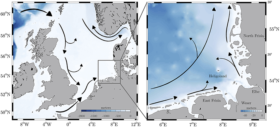
Figure 1. Major mean current pattern in the North Sea (Left) and in the German Bight (Right) (based on Otto et al., 1990).

The physical dynamics of the North Sea are mainly influenced by semidiurnal tidal forces (M₂), winds, and density and pressure gradients. The most dominant feature of the current pattern in the North Sea is the cyclonic residual circulation, which is caused by non-linear tidal interaction and prevailing westerly wind stress forcing (Otto et al., 1990). Wind conditions have a major influence on surface currents and transport processes in the German Bight (Huthnance, 1991). Easterly wind forcing can result in the formation of recirculating gyres in the surface layer in front of the North Frisian coastline and can lead to the formation of sub-mesoscale eddies with spatial scales of 5–20 km (Dippner, 1993).

The two main water masses found in the German Bight are Continental Coastal Water (CCW) and central North Sea Water (NSW). CCW is a combination of Atlantic water from the English Channel and the run-off from the rivers Scheldt, Rhine, Meuse, Ems, Elbe, and Weser (Becker et al., 1992). NSW in the northern part of the German Bight is strongly influenced by oceanic water with salinities above 33 PSU and is characterized by seasonal stratification (Huthnance, 1991). The bulk of oceanic water in the German Bight is delivered through the English Channel. During the transport along the coast, these water masses are influenced by the runoff from the rivers Scheldt, Rhine, Ems, Weser, and Elbe. Freshwater from these rivers dilutes the coastal waters (Becker et al., 1992). Elbe, Weser, and Ems create an estuarine frontal system, which affects a large area in the German Bight. In the eastern part of the German Bight, close to the North Frisian coast, the combination of riverine freshwater and saline water, which is transported by southwesterly winds into the German Bight, leads to a frontal zone with a strong haline gradient (Becker et al., 1999; Skov and Prins, 2001). That results in strong density gradients which can concentrate floating materials like FML along the density front (Carlson et al., 2018; D'Asaro et al., 2018).

Drifter Design

The drifter (Figure 2) was designed for use in coastal areas and tidal inlets to follow surface currents (~0.5 m depth). One of the design requirements was for the drifter housing to be small, making it possible to deploy in shallow waters and from small boats. Furthermore, the drifter had to be compact and light-weight to minimize storage space, allow easy handling during deployment, recovery and shipment. The drifter housing made of 6.7 mm thick polyvinyl chloride (PVC) consists of two main compartments of varying diameters (Figure 2). The upper part of the housing has a Styrofoam ring attached for positive buoyancy and maintaining the upright position of the drifter in water. This upper part is 135 mm in length and 140 mm in diameter, housing the positioning and telemetry module (Figure 2a). The lower part of the hull is 370 mm in length and 90 mm in diameter. It houses the battery pack at the base, which also helps to keep the drifter in an upright position. The design allows for the attachment of additional weights at the base to ballast the drifter (Figure 2c). The overall weight of the drifter is <5 kg.

FIGURE 2

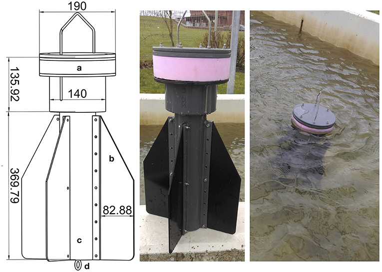
Figure 2. Drifter design: (a) buoyant part of the housing which contains the GPS-position and signal transmission unit, (b) exchangeable drag-reducing wings, (c) lower part of the housing which contains the battery pack and additional ballast, (d) ring screw for optional mounting of an external subsurface drogue. Dimensions are given in mm.

A small draft was also a pre-requisite of the design for investigations of complex motion processes in the coastal area and for studying the transport through the surf zone to the coastline. To this end, the drogue was attached to the lower part of the housing (Figure 2c). The drogue consists of four polyethylene (PE) drag-producing cruciform wings that are easy to attach or detach. There is a possibility to mount wings of varying sizes and shapes, enabling very accurate regulation of the wind slip for the drifter. An additional ring screw is mounted at the bottom of the housing which offers the possibility to attach a subsurface drogue to the drifter.

Positioning and Telemetry

Commercial off-the-shelf GPS receivers (SPOT Trace^®), which were successfully used in surface drifter experiments in the Gulf of Mexico (Novelli et al., 2017), were chosen because of their low-cost satellite fee and good global coverage of 96%. The accuracy of the GPS unit was determined by comparing 2,000 recorded coordinates that were taken at a fixed position determined by a differential GPS device over 2 weeks. The results are shown in a cumulative histogram, indicating that the position error is <2.5 m in 95% of the recorded positions (Figure 3a). The experiment was conducted for static conditions and the results may differ under oceanic conditions. It is noted that the cumulative position error may increase to ratios 20–60 times higher for drifter dispersion estimates (Haza et al., 2014). The satellite telemetry module transmits the geo-location of the drifters in near-real time via the Globalstar^® satellite network. Due to the compact design with the physical dimensions of 68 × 51 × 10 mm and a mass of 88 g, it can easily be accommodated in the housing. The device can transmit its position at intervals of 5, 10, 30, and 60 min using a simplex data modem. The sampling interval can be set by the user. If no position can be determined—for instance due to poor satellite reception—within 4 min, the SPOT Trace^® will try to determine a position at the next programmed tracking interval. In the case of no satellite connection, the device will store the coordinates until a successful transmission. For the presented experiments the sampling interval was set to 10 min to extend battery lifetime, as 10 min is an adequate resolution for the investigation of sub-mesoscale processes. To determine the tracking interval of the device, the time intervals of all transmitted positions were plotted in a cumulative histogram (Figure 3b). The results indicate that more than 80% of the positions were transmitted within 10 min.

FIGURE 3

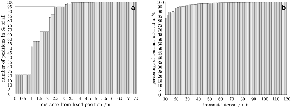
Figure 3. Position accuracy (a) and transmission interval (b) shown in a cumulative histogram. For the position accuracy test the number of positions in percent of all positions are plotted against the distance from the fixed position (b). The dashed line shows the 95th percentile and indicates that 95% of the positions have an error <2.5 m. The cumulative histogram for the transmission accuracy test shows the percentage of the transmission interval of all transmissions from all drifters as a function of the transmission interval.

In general, sub-mesoscale processes are in the range of days; this means power supply should last for at least several days or even longer. Longer power supply provides long-term datasets that can be used to study weekly, monthly or even seasonal transport patterns. The Spot Trace^® was powered by an external battery pack consisting of 8 D-cell alkaline batteries which extended the operational time of the drifter to about 9 months, with geo-location data transmission every 10 min. Each drifter, including the data plan for satellite data transmission, costs about US$ 300. The drifters are designed to be recovered and will be used in further experiments.

Wind Slip

The wind slip is the horizontal motion of a drifter that differs from the motion of the surface currents and is caused by the direct wind forcing on the surface float (Lumpkin and Pazos, 2007). The wind slip U_slip can be calculated as estimated in Suara et al. (2015) and Carlson et al. (2017a) by

$\begin{array}{l}{\text{U}}_{\text{s}li\text{p}}=\frac{\text{A}}{\text{R}}{\text{U}}_{\text{W}in\text{d}}\end{array}$

where U_Wind is the wind velocity at a height of 10 m above the sea level and A is 0.07 (Niiler and Paduan, 1995). R is the drag area ratio (DAR) and is defined as

$\begin{array}{l}\text{R}=\frac{{\text{C}}_{\text{w}}{\text{A}}_{\text{w}}}{{\text{C}}_{\text{a}}{\text{A}}_{\text{a}}}.\end{array}$

C_a represents the drag coefficient of the elements of the float above the water surface and which are exposed to the air and C_w indicates the drag coefficient of the elements below the water surface. A_a and A_w are the values for the cross-sectional area above and below the water surface. The cross-sectional areas above and below the water's surface of the present drifter configuration were determined in a pool with sea water with a salinity of 34 PSU. The drag area ratio is R = 25.6 due to its cross-sectional area of 62.3 cm² above and 1194.6 cm² below the water surface. Subsequently, the downwind slip U_slip of the drifter is 0.27% of the wind speed. As an example, the wind-induced slip resulting from wind speeds in a range of 1–10 m s⁻¹ would be 0.0027–0.027 m s⁻¹ in a downwind direction. For different scientific questions, the drag area ratio can be easily adjusted by replacing the vanes or by attaching an external subsurface drogue to a ring screw which is mounted to the bottom of the housing.

Drifter Data Processing

Latitude and longitude data in degrees were converted to the universal transverse Mercator coordinate system (UTM), giving the position of a drifter in zonal and meridional coordinates (X_d(t), Y_d(t)). Missing data due to data transmission errors or positioning errors longer than 120 min were flagged in the dataset and not used for further analysis. Two drifters have shown data gaps longer than 120 min. The percentage of the missing data is 0.27% for drifter D2 and 0.03% for drifter D3.

Outliers in the drifter position time series data were eliminated with a Hampel median filter for zonal and meridional coordinates separately (Liu et al., 2004). The filter computes for every sample the median and the standard deviation for a window of the 18 surrounding samples (9 per side). All sample values that differ from the median by more than three standard deviations are removed from the time series dataset of drifter positions. Since drifter positions were measured at irregular time intervals, the position data were interpolated using a piecewise cubic interpolation method (Fritsch and Carlson, 1980), creating a consistent data output at 10 min intervals for further velocity and tidal analysis.

Velocity Calculation

Zonal and meridional velocity components were determined with a forward difference scheme:

$U_d=\frac{X_d\left(t+\delta t\right)-X_d(t)}{\delta t}$

and

$V_d=\frac{Y_d\left(t+\delta t\right)-Y_d(t)}{\delta t}$

where U_d is the drifter velocity in the zonal direction and V_d represents the meridional drifter velocity component.

Tidal Analysis

Percent energy (PE) is an important indicator that can explain the significance of each tidal constituent (Codiga, 2004). The tidal harmonic analysis toolbox UTide was implemented for the analysis of the tidal constituents (Codiga, 2011). The most dominant tidal constituent is the principal lunar semi-diurnal tide M₂ and the solar semi-diurnal tide S₂, with values between 90 and 95 percent energy, for the analyzed velocity time series data. In addition, the velocity time series data of the drifters were decomposed into their respective frequencies using a Fast Fourier Transformation (FFT). The FFT also shows the dominance of the semi-diurnal tidal constituents M₂ and S₂ (Figure 4). To remove the tidal zonal (U_tide) and meridional (V_tide) current velocities, the time series data of the current velocity were low-pass filtered with a moving average filter over the period of 24.83 h.

FIGURE 4

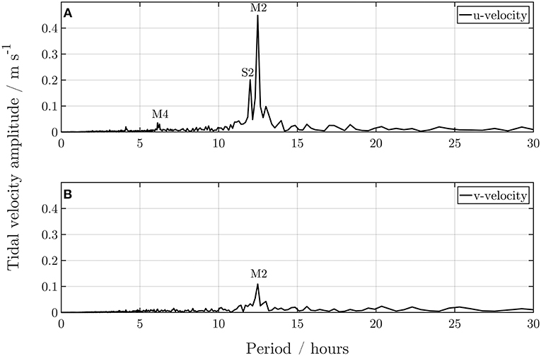
Figure 4. Spectral analysis of the zonal (A) meridional (B) drifter velocities using a Fast Fourier Transformation (FFT).

The residual zonal (U_res) and meridional (V_res) velocities were determined as follows

$\begin{array}{l}{\text{U}}_{\text{res}}={\text{U}}_{\text{d}}-{\text{U}}_{\text{tide}}\end{array}$

and

$\begin{array}{l}{\text{V}}_{\text{res}}={\text{V}}_{\text{d}}-{\text{V}}_{\text{tide}}\end{array}$

where U_d and V_d are the drifter velocities in the zonal and meridional direction, respectively.

Wind Data

Wind data used in this study were taken from the meteorological station of the German Weather Service (DWD) located on Heligoland. Wind speed and direction is measured in an hourly resolution with an ultrasonic anemometer installed 10 m above sea level. The wind direction is measured with a 36-part wind rose. To investigate the correlation between drifter and wind speeds, a grid of zonal and meridional wind speeds that occurred in the deployment period with an interval of 2 ms⁻¹ was defined. The corresponding residual drifter velocities for each bin on the grid were averaged for every deployed drifter separately. As an example, all residual zonal drifter velocities that occurred during zonal wind speeds of 4–6 ms⁻¹ were identified by the corresponding timestamp and were averaged for every drifter separately. The bin-averaged residual velocities were plotted against the averages of the corresponding wind velocities for each drifter residual velocity bin. The minimum sample size for each bin-average is 6, so that all samples below that sample size were not considered in the analysis. By averaging the individual residual drifter velocities to the corresponding wind speed bin, it was possible to compare the drifter residual velocities to the local wind field and mitigate the noise in the drifter residual velocity dataset that was generated by rapidly changing gusts of wind.

Results

A total of four drifters were deployed in March 2017 and 3 drifters were deployed in October 2017 from RV Heincke and RV Senckenberg. These deployments were done in 3 pairs, at the same time, with an initial separation of <1 m except for drifter 7. Deployment locations were chosen to be in the coastal area near the major shipping lane as a possible source for FML in the German Bight. Metadata related to these drifter deployments, beaching and drifter displacement are summarized in Table 1. The lifetimes of the drifters deployed in March 2017 ranged from 22 to 39 days.

TABLE 1

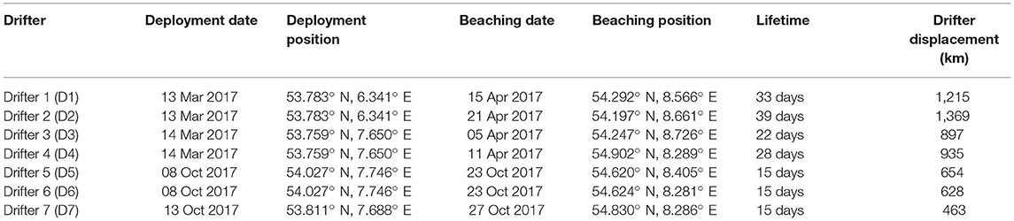
Table 1. Summary of the drifter deployments in March and October 2017.

All drifters launched in October 2017 had lifetimes of 15 days. The average meridional speeds of the drifters deployed in March 2017 ranged from 0.019 to 0.051 ms⁻¹ and the average zonal speeds ranged from 0.013 to 0.052 ms⁻¹. In October 2017, average meridional speeds were in the range of 0.026 to 0.033 ms⁻¹ whilst average zonal drifter speeds were from 0.051 to 0.089 ms⁻¹. Wind direction distributions for the March (Figure 5A) and October (Figure 5B) deployments are presented as a wind rose histogram in direction of the blowing wind. The general wind direction for the March deployment was mostly southeastwards, with wind speeds ranging from 5 ms⁻¹ to 12 ms⁻¹ and maximum speeds reaching 16.8 ms⁻¹. Wind speeds in October were higher, ranging from 8 ms⁻¹ to 14 ms⁻¹ and peak speeds of up to 24.3 ms⁻¹. The predominant wind direction in October was toward the northeast.

FIGURE 5

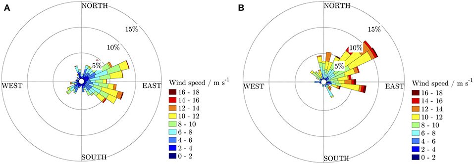
Figure 5. Distribution of wind speed and direction measured at the DWD weather station in Heligoland during the March 2017 drifter deployments (A) and for the October 2017 drifter deployment (B). The wind direction is displayed in the direction of the blowing wind and the color code refers to the wind speed in ms⁻¹.

The individual trajectories of the drifters deployed in March are shown in Figure 6 with a different color for consecutive five-day intervals. The corresponding colored arrows illustrate the average wind conditions for these time intervals to give an overview of the wind forcing in these time periods. Drifter 1 (D1) and Drifter 2 (D2) were deployed on the 13th of March 2017 at the border of the German Exclusive Economic Zone to the northwest of Borkum (Figures 6a,b). In the beginning, the drifter pair moved eastward due to stable westerly winds. The further course of the trajectories is mainly influenced by semi-diurnal tidal oscillations and wind forcing. Due to principal westerly winds during the deployment interval, D1 beached at the North Frisian coastline 33 days after the release with a displacement of 1,215 km. D2 washed ashore 39 days after deployment not far away from the beaching location of D1 and covered a distance of 1,369 km. Drifters 3 (D3) and 4 (D4) were deployed in the tidal inlet between the islands Spiekeroog and Langeoog on the 14th of March 2017 (Figures 6c,d). However, both drifters were transported to the east by stable westerly winds during the first days after the deployment. The trajectories were split up in front of the Elbe estuary 5 days after the deployment. D3 was trapped in a tidal eddy in front of the North Frisian coastline for almost 12 days before the drifter stranded in the North Frisian Wadden sea (Supplementary Video 1). The drifter covered a distance of 897 km in a period of 22 days. D4 washed ashore in the Wadden Sea in front of the island Scharhörn during flood tide on the 19th of March 2017 (Supplementary Video 1 and Supplementary Figure 1). The drifter was flushed back into the sea on the 20th of March at high tide and strong southwesterly winds (15 ms⁻¹), passed the Elbe estuary and was transported to the northwest and stranded 28 days after deployment on the island Sylt (Supplementary Video 1). The drifter covered a distance of 935 km on its journey. It was the only drifter that stranded and refloated.

FIGURE 6

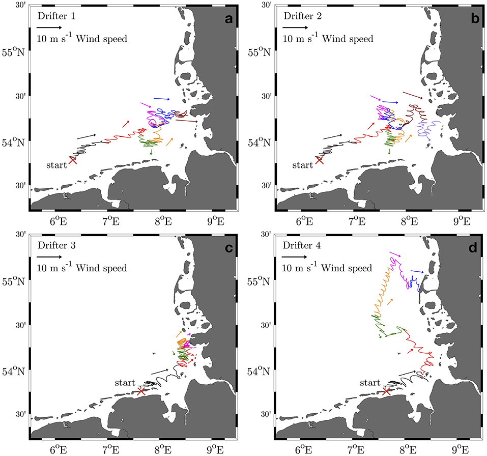
Figure 6. Trajectories of 4 drifters deployed in March 2017. (a–d) The release location is indicated by a red cross for every trajectory. The trajectories were subdivided into 5-day segments, which are indicated by different colors. The corresponding colored arrows show the mean prevailing wind directions for the associated 5-day segments.

The trajectories of the drifters from the October deployment are shown in Figure 7. Drifter 5 (D5) and Drifter 6 (D6) were deployed as a pair on the 8th of October 2017, southwest of the island Heligoland (Figures 7a,b). The trend of the pathways of D5 and D6 are very similar in the beginning. Due to strong winds from the west, the drifters moved in 5 days to the northern part of the Elbe estuary. From there, they were transported northward along the North Frisian coast. The drifters meandered for 7 days close to the North Frisian Islands and were flushed several times with the tidal currents into the tidal inlets before they stranded on the island Amrum (Supplementary Video 2). Both drifters D5 and D6 beached 15 days after their release. D5 covered a distance of 654 km, whereas D6 traveled a distance of 628 km in the German Bight. Drifter 7 (D7) was deployed north of the island Spiekeroog on the 13th of October 2017 (Figure 7c). Due to strong southwesterly winds, the drifter moved in the northeastern direction. A week after the deployment, D7 passed the island Heligoland and was transported northwards by strong winds from the south. Drifter D7 stranded on the island Sylt 15 days after release and covered a distance of 463 km on its journey. All drifters discussed in this study were immediately recovered by tourists on beaches or in dry falling areas in the Wadden sea after the experiments.

FIGURE 7

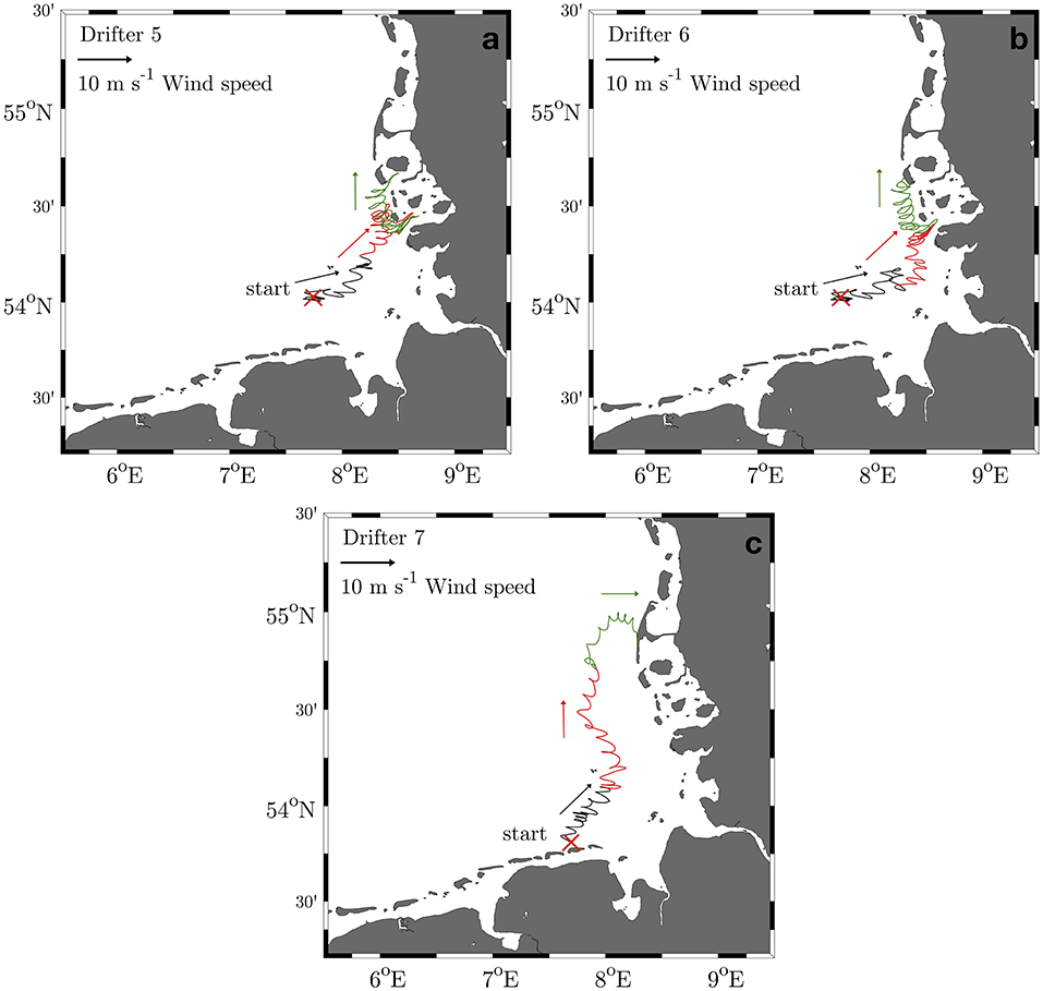
Figure 7. Trajectories of 3 drifters deployed in October 2017. (a–c) The release location is indicated by a red cross for every trajectory. The trajectories were subdivided into 5-day segments which are indicated by different colors. The corresponding colored arrows show the mean prevailing wind directions for the associated 5-day segments.

To illustrate observed and derived parameters, the zonal (U_d) and meridional (V_d) drifter velocities, estimated tidal velocities (zonal U_tide, meridional V_tide) and residual velocities (zonal U_res, meridional V_res) of D1 and D2 are presented in Figure 8. Values for U_d for D1 range from −1.08 ms⁻¹ to 1.19 ms⁻¹ and the zonal velocity values for D2 vary from −0.86 ms⁻¹ to 1.28 ms⁻¹. The tidal oscillation of the drift velocities is pronounced in the time series data and spring-neap tidal cycles are significant. The dominance of the M₂ signal can be identified in the zonal velocities and is more prominent than in the meridional velocities. The tidal oscillations are independent of calm or stormy weather events. The amplitude of the meridional velocity components is lower in comparison to the zonal components. Low-pass-filtered residual currents have a zonal velocity amplitude of −0.29 ms⁻¹ to 0.30 ms⁻¹ for D1 and −0.23 ms⁻¹ to 0.41 ms⁻¹ for D2. The meridional velocity amplitudes of the drifters are smaller in comparison to the zonal velocities, which range from −0.77 ms⁻¹ to 0.59 ms⁻¹ for D1 and −0.48 ms⁻¹ to 0.66 ms⁻¹ for D2. The low-pass-filtered residual meridional velocities vary from −0.23 ms⁻¹ to 0.24 ms⁻¹ for D1 and from −0.27 ms⁻¹ to 0.33 ms⁻¹ for D2.

FIGURE 8

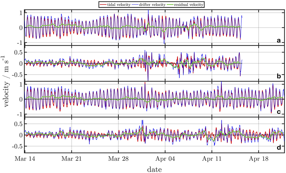
Figure 8. Time series of drifter-derived velocities (blue line) of D1 of the zonal component (A) and the meridional component (B) and D2 (C,D). The estimated tidal velocities are indicated by the red line and the residual velocities are highlighted as a green line.

Figure 9 provides an overview of the drifter velocities, the tidal velocities and the residual velocities for the October deployment (D5 and D6). U_d shows similar magnitudes in comparison to D1 and D2. V_d is significantly higher in comparison to D1 and D2 with values in a range from −1.12 ms⁻¹ to 1.01 ms⁻¹ for D5 and −0.91 ms⁻¹ to 0.96 ms⁻¹ for D6. The highest values in both velocity components were observed in the tidal inlet in front of the North Frisian coast. The derived residual velocities range from −0.15 ms⁻¹ to 0.31 ms⁻¹ for D5 and −0.15 ms⁻¹ to 0.25 ms⁻¹ for D6 regarding the zonal component. V_res varies from −0.19 ms⁻¹ to 0.22 ms⁻¹ for D5 and from −0.20 ms⁻¹ to 0.18 ms⁻¹ for D6. The influence of the tidal oscillation is significant for the drifter velocities. The amplitudes of the velocity components are significantly higher for the spring tide period, which occurred on the 19th of October 2017.

FIGURE 9

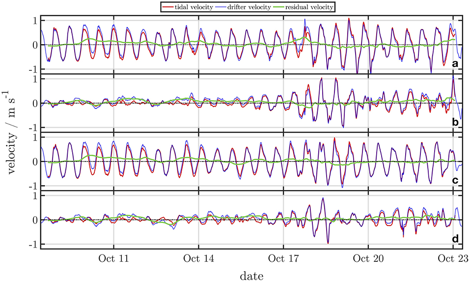
Figure 9. Time series of drifter-derived velocities (blue line) of D5 of the zonal component (A) and the meridional component (B) and D6 (C,D). The estimated tidal velocities are indicated by the red line and the residual velocities are highlighted as a green line.

Statistically significant positive linear correlations (R² > 0.72, p < 0.05) between bin-averaged wind velocities and bin-averaged residual drifter velocities for all 7 drifters were observed (Figure 10). The correlation between bin-averaged winds and residual drifter velocities has a strong positive association (Figure 10A, R² = 0.72, N = 98, RMSE = 4.5 cm s⁻¹ for the zonal component; Figure 10B, R² = 0.86, N = 98, RMSE = 3.6 cm s⁻¹ for the meridional component).

FIGURE 10

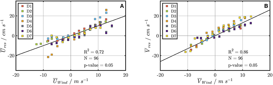
Figure 10. Bin-averaged residual drifter zonal (A) and meridional (B) velocities as a function of the bin-averaged wind speed for every drifter separately. The slope of the fit in (A) is 1 and shows the bin-averaged zonal velocity as a function of the zonal wind speed component with squared correlation of R² = 0.72 and p = 0.05. The slope of the fit in (B) is 1.3 and shows the bin-averaged meridional velocity as a function of the meridional wind speed component with squared correlation of R² = 0.86 and p = 0.05.

Discussion

The state-of-the-art low-cost drifter design presented here is primarily intended for use in shallow waters but can be easily adapted to all the above-mentioned scientific questions for the open ocean environment. The drag area ratio can be adjusted by changing the vanes and regulating the draft of the housing. Due to the low draft, the drifter can operate in estuaries and in surf zones to measure rip currents. The possibility to attach a subsurface drogue to a ring screw at the bottom of the housing enables the drifter to provide valuable information on the large-scale ocean circulation for deep-water surveys.

Positioning (Figure 2a) and data transmission (Figure 2b) analysis have shown that the drifter observations provide accurate geo-location and high temporal data that are necessary to resolve sub-mesoscale processes. The positions were transmitted at an average interval of 12.4 min with very minimal data gaps. A major disadvantage is the fact that no other sensors can be connected directly to the SPOT Trace^®. The drifter deployments in October suggest that the drifters can operate and provide reliable data during stormy weather conditions with wind speeds up to 24.3 ms⁻¹ and resulting high waves. Due to the robust drifter design, it is therefore also possible to observe transport patterns of floating objects during storm events.

The drifter design is capable of representing beaching and refloating comparable to floating marine litter of a certain size. The beaching and refloating processes are very challenging issues which are poorly represented in most marine litter transport models (Critchell et al., 2015). Beaching of floating objects strongly depends on the buoyancy of the objects (Yoon et al., 2010), the structure of the coastline, winds, waves, tides and the bathymetry (Critchell et al., 2015).

The trajectories of D1 and D3 show a beaching scenario in the same coastal area under different wind conditions. D1 meandered in coastal waters for 12 days due to very low wind speeds of 1–3 ms⁻¹, whereas D3 washed ashore near the stranding location of D1 but passed through the coastal area in 2 days due to westerly wind speeds of approximately 10 ms⁻¹. Refloating of beached objects due to tides and winds is shown in the trajectory of D4, which was the only drifter that beached and refloated, because the other drifters were immediately recovered by tourists. The drifter washed ashore and was resuspended into the ocean a day later by strong southwesterly winds and tides. The dispersion of D3 and D4 is caused by the stranding and refloating of D4. Refloating of objects in a complex tidally influenced shallow water area represents an important process regarding the transport pattern and stranding locations of FML and needs to be taken into account in particle tracking models.

The trajectories of D3, D5, and D6 indicate that floating items tend to accumulate in sub-mesoscale tidal recirculation cells under low wind conditions. The formation of recirculation cells due to calm wind conditions in the eastern part of the German Bight (Dippner, 1993) can lead to significantly longer residence times of FML along the North Frisian coastline. The residence times can be calculated by computing the characteristic time of a drifter in a specified spatial domain (Choukroun et al., 2010). Dippner (1998) also discussed the formation of three mesoscale eddies between the salinity front of the river plumes of the Elbe and Weser and the North Frisian coast during westerly wind conditions caused by the interaction of wind stress and the gradient of the bottom topography. This eddy regime can result in a disintegration of the northward transport between the salinity front and the coast and can lead to accumulation and longer residence times of FML in this area. The residence times of D3, D5, and D6 in the coastal area in front of the North Frisian shoreline support these assumptions. Observations by Thiel et al. (2011) have shown a higher abundance of flotsam in the coastal area, which is influenced by estuarine frontal systems and by intermittent eddies, than in areas farther offshore, which is also in a good agreement with the residence times of D3, D5, and D6. Gutow et al. (2018) observed also very high densities of FML along the North Frisian coastline with values above 100 items km⁻², which fits well with our findings.

Furthermore, several studies reported on the accumulation of floating objects at frontal systems (Skov and Prins, 2001; Acha et al., 2003; Pichel et al., 2007; Thiel et al., 2011; Gutow et al., 2018), which is an important factor regarding the transport pattern of FML and needs to be focused on in further investigations. If floating objects remain for longer periods in frontal areas, the objects can lose their buoyancy due to marine fouling and sink to the ground or are pushed with winds to the shore (Hinojosa et al., 2011). In addition, it has been reported that bottom litter might accumulate in areas with high sediment transport and low circulation rates (Galgani et al., 2000), which could also be an important factor regarding the accumulation of marine litter in the German Bight due to high sedimentation rates in the North Frisian and East Frisian areas (Lettmann et al., 2009; Zeiler et al., 2014).

The complex interaction of tides, winds and the coastline structure in the coastal area is demonstrated by the trajectories of D5 and D6. The drift patterns of both drifters are significantly influenced by strong tidal jets in the tidal inlets in front of the North Frisian coast. The drifters were flushed several times into the tidal inlets with the flood tide and floated back in front of the islands with the ebb tide, which gives rise to the assumption that floating objects can also be trapped for longer time periods in the vicinity of tidal inlets.

The drifter velocities are dominated by tides, wind induced slippage and surface currents (Figures 4, 10). The tidal components are clearly pronounced in the zonal velocities whereas the tidal oscillations in the meridional component seem to be more irregular (Figures 8, 9). Similar results were also found in high frequency radar data (HF-radar) and model results for the German Bight, which show that the tidal ellipses are very pronounced in the zonal direction (Barth et al., 2010; Port et al., 2011). The tidal analysis shows that the most dominant tidal constituents in the surface velocity field are the principal lunar semi-diurnal tide M₂ and the solar semi-diurnal tide S₂. These findings are consistent with numerical simulations and HF-radar observations (Port et al., 2011). Magnitudes of zonal and meridional velocities agree with HF-radar-derived velocities in this area (Port et al., 2011; Stanev et al., 2015). The residual velocities are significantly correlated with the local wind fields (Figure 10). The fit parameters and the correlation coefficients show a stronger wind influence on the meridional component, which is in good agreement with results shown by Port et al. (2011). The wind-induced drifter movement is driven by the direct wind slippage (Section Wind Slip), wind stress on the surface current and the Stokes drift. The variance observed in the zonal velocities at high wind speeds could be caused by increasing crosswind leeway components which need to be taken into account at high wind speeds (Breivik et al., 2011). Furthermore, island effects have a major impact on velocity fields in the coastal area and need also to be taken into account. The findings of this study indicate, that tidal jet currents have an enormous impact on the sediment transport in the coastal zone (Staneva et al., 2009). Mantovanelli et al. (2012) have shown, that strong jet currents which are generated by the bathymetry in the coastal area and tidal channels between islands, have significant influence on the transport of particles in the coastal area. This agrees well with the observations of this study, which also show the highest drifter velocities for both components in tidal inlets generated by tidal jets (Figure 9, and Supplementary Video 2) which seem to overshadow the wind effects in the coastal area. These findings are also in good agreement with recent studies by Callies et al. (2017) that compared trajectories of six surface drifters with results of offline particle simulations in the inner German Bight.

Overall, the analysis of the drifter velocities shows that the transport of floating objects at the ocean surface is strongly affected by the local wind field, especially for areas far away from the coast. The wind data is taken from a single observational station and is not representative for the whole region of the study, but due to its central location in the German Bight it can give a good estimate of the local wind field. Laxague et al. (2018) have demonstrated, that the transport of floating objects at the surface is predominantly forced by wind- and wave-induced motions and that the currents at the surface (0.001–0.5 m) are significantly stronger compared to the surface currents averaged over the top 5 m of the water column. Most particle tracking models poorly represent these wind- and wave-induced motions at the surface or do not have adequate resolution to describe the transport processes of floating items at the surface accurately (Laxague et al., 2018). The drifter design presented in this study is targeted at the motion processes of floating items in the surface layer (0.5 m) and takes into account wind- and wave-induced motions in this small vertical column having an enormous impact on the transport pattern of FML. These results could be useful for the parametrization of wind- and wave- induced motions of surface currents in particle tracking models, which has been recently demonstrated by Stanev et al. (Forthcoming). Since the residence time of FML strongly depends on the buoyancy ratio of floating objects (Yoon et al., 2010), experiments with different drag area ratios can be very helpful for the validation of particle tracking models. The presented drifter setting with a drag area ratio of 25.6 represents macroscopic litter that floats at the sea surface with a low buoyancy. SVP drifters with drag area ratios around 40 represent typically the current of the first 20 meters of the surface layer. The movement of macroscopic litter takes place in the upper 0.5 m of the ocean and is strongly influenced by wind- and wave-induced forces (Laxague et al., 2018). Lagrangian drifter experiments with different drag area ratios can provide fundamental insights into the dynamics of FML of different shapes at the ocean's surface.

The combination of wind-induced motion and nearshore processes like tidal jets, the formations of sub-mesoscale recirculation cells and the interaction with a complex shoreline have a great impact on the pathways, accumulation, residence times and beaching of floating objects in the German Bight. The investigation of these processes is fundamental for understanding the beaching behavior of FML at the shoreline and to implement such processes in high resolution particle tracking models (Neumann et al., 2014; Schulz and Matthies, 2014; Schulz et al., 2015b).

Conclusions

The drifter design presented in this study was primarily developed for the observation of the transport of floating objects in shallow waters, with an adjustable drag area ratio which is 25.6 for the presented configuration. The drifter is compact, robust, accurate, affordable, simple to manufacture and is easily adaptable to address open ocean and coastal water questions related to transport pattern of pollutants and current circulation studies. The trajectories of these drifters generate information on the surface current velocity field and complex transport patterns from the coastal area to the open sea. Here we present findings from seven surface drifters deployed in the German Bight, a region with a substantial lack of Lagrangian observations. Our drifter-derived surface current velocity data and resolved transport patterns in the coastal area were consistent with hydrodynamical and particle tracking simulations in the German Bight. The direct wind slip of the drifter was determined to be 0.27% of the wind speed, and the overall wind induced motion to the drifter due to waves, direct wind slip and wind stress at the water surface was about 1% of the wind speed.

The drifter trajectories observed in this study highlight some of the constraints in simulating the transport of FML in the open ocean and even more in coastal zones. The processes presented in this study need to be taken into account to better represent the transport of FML in numerical simulations in a more realistic approach, which will be done in further work with a nested high-resolution particle tracking model. Ultimately, the typical movement of particles in water is a Lagrangian problem, which needs to be better understood with the aid of accurate in situ Lagrangian observations.

Author Contributions

JM and TB contributed to the data collection and the data analysis. JM drafted the manuscript and all other authors contributed to the critical revision of the article and provided important advice for the improvement of the manuscript. All authors were involved in the conception of the experiments.

Funding

This study was carried out within the project Macroplastics Pollution in the Southern North Sea–Sources, Pathways and Abatement Strategies (Grant ZN3176) funded by the German Federal State of Lower Saxony.

Conflict of Interest Statement

The authors declare that the research was conducted in the absence of any commercial or financial relationships that could be construed as a potential conflict of interest.

Acknowledgments

We would like to thank Axel Braun, Michael Butter and Andreas Sommer for the support in constructing the drifters and Helmo Nicolai, Gerrit Behrens, and Waldemar Siewert and the master and crew onboard the RV Heincke HE 498 for supporting the deployments of the drifters. We thank Marcel Ricker for comments on the manuscript and providing some important advice. Many thanks go to Michael Norie for language editing. We would like to thank the two reviewers and the editor Dr. Gilles Reverdin for very useful comments.

Supplementary Material

The Supplementary Material for this article can be found online at: https://www.frontiersin.org/articles/10.3389/fmars.2019.00058/full#supplementary-material

References

Acha, E. M., Mianzan, H. W., Iribarne, O., Gagliardini, D. A., Lasta, C., and Daleo, P. (2003). The role of the Rio de la Plata bottom salinity front in accumulating debris. Mar. Pollut. Bull. 46, 197–202. doi: 10.1016/S0025-326X(02)00356-9

PubMed Abstract | CrossRef Full Text | Google Scholar

Barnes, D. K., Galgani, F., Thompson, R. C., and Barlaz, M. (2009). Accumulation and fragmentation of plastic debris in global environments. Philos. Trans. R. Soc. Lond. B Biol. Sci. 364, 1985–1998. doi: 10.1098/rstb.2008.0205

PubMed Abstract | CrossRef Full Text | Google Scholar

Barth, A., Alvera-Azcárate, A., Gurgel, K.-W., Staneva, J., Port, A., Beckers, J.-M., et al. (2010). Ensemble perturbation smoother for optimizing tidal boundary conditions by assimilation of High-Frequency radar surface currents – application to the German Bight. Ocean Sci. 6, 161–178. doi: 10.5194/os-6-161-2010

CrossRef Full Text | Google Scholar

Baschek, B., Schroeder, F., Brix, H., Riethmüller, R., Badewien, T. H., Breitbach, G., et al. (2017). The Coastal Observing System for Northern and Arctic Seas (COSYNA). Ocean Sci. 13, 379–410. doi: 10.5194/os-13-379-2017

CrossRef Full Text | Google Scholar

Becker, G. A., Dick, S., and Dippner, J. W. (1992). Hydrography of the German Bight. Mar. Ecol. Prog. Ser. 91, 9–18. doi: 10.3354/meps091009

CrossRef Full Text | Google Scholar

Becker, G. A., Giese, H., Isert, K., König, P., Langenberg, H., Pohlmann, T., et al. (1999). Mesoscale structures, fluxes and water mass variability in the German Bight as exemplified in the KUSTOS- experiments and numerical models. Dtsch. Hydrogr. Z. 51, 155–179. doi: 10.1007/BF02764173

CrossRef Full Text | Google Scholar

Bergmann, M., Sandhop, N., Schewe, I., and D'Hert, D. (2016). Observations of floating anthropogenic litter in the Barents Sea and Fram Strait, Arctic. Polar Biol. 39, 553–560. doi: 10.1007/s00300-015-1795-8

CrossRef Full Text | Google Scholar

Breivik, Ø., Allen, A. A., Maisondieu, C., and Olagnon, M. (2013). Advances in search and rescue at sea. Ocean Dyn. 63, 83–88. doi: 10.1007/s10236-012-0581-1

CrossRef Full Text | Google Scholar

Breivik, Ø., Allen, A. A., Maisondieu, C., and Roth, J. C. (2011). Wind-induced drift of objects at sea: the leeway field method. Appl. Ocean Res. 33, 100–109. doi: 10.1016/j.apor.2011.01.005

CrossRef Full Text | Google Scholar

Callies, U., Groll, N., Horstmann, J., Kapitza, H., Klein, H., Maßmann, S., et al. (2017). Surface drifters in the German Bight: model validation considering windage and Stokes drift. Ocean Sci. 13, 799–827. doi: 10.5194/os-13-799-2017

CrossRef Full Text | Google Scholar

Carlson, D. F., Boone, W., Meire, L., Abermann, J., and Rysgaard, S. (2017a). Bergy bit and melt water trajectories in Godthåbsfjord (SW Greenland) observed by the expendable ice tracker. Front. Mar. Sci. 4:276. doi: 10.3389/fmars.2017.00276

CrossRef Full Text | Google Scholar

Carlson, D. F., Özgökmen, T., Novelli, G., Guigand, C., Chang, H., Fox-Kemper, B., et al. (2018). Surface ocean dispersion observations from the ship-tethered aerostat remote sensing system. Front. Mar. Sci. 5:479. doi: 10.3389/fmars.2018.00479

CrossRef Full Text | Google Scholar

Carlson, D. F., Suaria, G., Aliani, S., Fredj, E., Fortibuoni, T., Griffa, A., et al. (2017b). Combining litter observations with a regional ocean model to identify sources and sinks of floating debris in a semi-enclosed basin: the Adriatic Sea. Front. Mar. Sci. 4:78. doi: 10.3389/fmars.2017.00078

CrossRef Full Text | Google Scholar

Choukroun, S., Ridd, P. V., Brinkman, R., and McKinna, L. I. W. (2010). On the surface circulation in the western Coral Sea and residence times in the Great Barrier Reef. J. Geophys. Res. 115, 1–13. doi: 10.1029/2009JC005761

CrossRef Full Text | Google Scholar

Claessens, M., Meester, S. D., Landuyt, L. V., Clerck, K. D., and Janssen, C. R. (2011). Occurrence and distribution of microplastics in marine sediments along the Belgian coast. Mar. Pollut. Bull. 62, 2199–2204. doi: 10.1016/j.marpolbul.2011.06.030

PubMed Abstract | CrossRef Full Text | Google Scholar

Codiga, D. L. (2004). Observed tidal currents outside Block Island Sound: offshore decay and effects of estuarine outflow. J. Geophys. Res. 109:C07S05. doi: 10.1029/2003JC001804

CrossRef Full Text | Google Scholar

Codiga, D. L. (2011). Unified Tidal Analysis and Prediction Using the UTide Matlab Functions. Graduate School of Oceanography, Tech. Rep. 2011-01, University of Rhode Island, Narragansett, RI.

Google Scholar

Critchell, K., Grech, A., Schlaefer, J., Andutta, F. P., Lambrechts, J., Wolanski, E., et al. (2015). Modelling the fate of marine debris along a complex shoreline: lessons from the Great Barrier Reef. Estuar. Coast. Shelf Sci. 167, 414–426. doi: 10.1016/j.ecss.2015.10.018

CrossRef Full Text | Google Scholar

D'Asaro, E. A., Shcherbina, A. Y., Klymak, J. M., Molemaker, J., Novelli, G., Guigand, C. M., et al. (2018). Ocean convergence and the dispersion of flotsam. Proc. Natl. Acad. Sci. U.S.A. 115, 1162–1167. doi: 10.1073/pnas.1718453115

PubMed Abstract | CrossRef Full Text | Google Scholar

Davis, R. (1985). Drifter observations of coastal surface currents during CODE: the method and descriptive view. J. Geophys. Res. Oceans 90, 4741–4755. doi: 10.1029/JC090iC03p04741

CrossRef Full Text | Google Scholar

Davis, R., Dufour, J., Parks, G., and Perkins, M. (1982). Two Inexpensive Current-Following Drifters. Scripps Inst. Oceanogr. Univ. Calif. San Diego. La Jolla, CA. SIO Ref.

Dippner, J. W. (1993). A frontal-resolving model for the German Bight. Cont. Shelf Res. 13, 49–66. doi: 10.1016/0278-4343(93)90035-V

CrossRef Full Text | Google Scholar

Dippner, J. W. (1998). Vorticity analysis of transient shallow water eddy fields at the river plume front of the River Elbe in the German Bight. J. Mar. Syst. 14, 117–133. doi: 10.1016/S0924-7963(97)00008-0

CrossRef Full Text | Google Scholar

Dixon, T. J., and Dixon, T. R. (1983). Marine litter distribution and composition in the North Sea. Mar. Pollut. Bull. 14, 145–148. doi: 10.1016/0025-326X(83)90068-1

CrossRef Full Text | Google Scholar

Eriksen, M., Lebreton, L. C., Carson, H. S., Thiel, M., Moore, C. J., Borerro, J. C., et al. (2014). Plastic pollution in the world's oceans: more than 5 trillion plastic pieces weighing over 250,000 Tons Afloat at Sea. PLoS ONE. 9:e111913. doi: 10.1371/journal.pone.0111913

PubMed Abstract | CrossRef Full Text | Google Scholar

Fritsch, F. N., and Carlson, R. E. (1980). Monotone piecewise cubic interpolation. SIAM J. Numer. Anal. 17, 238–246. doi: 10.1137/0717021

CrossRef Full Text | Google Scholar

G20 (2017). Annex to G20 Leaders Declaration: G20 Action Plan on Marine Litter G20 Summit. Hamburg: Federal Ministry for the Environment, Nature Conservation, Building and Nuclear Safety.

Galgani, F., Leaute, J., Moguedet, P., Souplet, A., Verin, Y., Carpentier, A., et al. (2000). Litter on the sea floor along European Coasts. Mar. Pollut. Bull. 40, 516–527. doi: 10.1016/S0025-326X(99)00234-9

CrossRef Full Text | Google Scholar

Garaba, S. P., Aitken, J., Slat, B., Dierssen, H. M., Lebreton, L., Zielinski, O., et al. (2018). Sensing ocean plastics with an airborne hyperspectral shortwave infrared imager. Environ. Sci. Technol. 52, 11699–11707. doi: 10.1021/acs.est.8b02855

CrossRef Full Text | Google Scholar

GESAMP (2015). “Sources, fate and effects of microplastics in the marine environment: a global assessment,” in (IMO/FAO/UNESCO-IOC/UNIDO/WMO/IAEA/UN/UNEP/UNDP Joint Group of Experts on the Scientific Aspects of Marine Environmental Protection). GESAMP Report and Studies No. 90. ed P. J. Kershaw (London: International Maritime Organization), 96.

Gutow, L., Ricker, M., Holstein, J. M., Dannheim, J., Stanev, E. V., and Wolff, J.-O. (2018). Distribution and trajectories of floating and benthic marine macrolitter in the south-eastern North Sea. Mar. Pollut. Bull. 131, 763–772. doi: 10.1016/j.marpolbul.2018.05.003

PubMed Abstract | CrossRef Full Text | Google Scholar

Haza, A. C., Özgökmen, T. M., Griffa, A., Poje, A. C., and Lelong, M.-P. (2014). How does drifter position uncertainty affect ocean dispersion estimates? J. Atmos. Oceanic Technol. 31, 2809–2828. doi: 10.1175/JTECH-D-14-00107.1

CrossRef Full Text | Google Scholar

Hinojosa, I. A., Rivadeneira, M. M., and Thiel, M. (2011). Temporal and spatial distribution of floating objects in coastal waters of central–southern Chile and Patagonian fjords. Cont. Shelf Res. 31, 172–186. doi: 10.1016/j.csr.2010.04.013

CrossRef Full Text | Google Scholar

Huthnance, J. (1991). Physical oceanography of the North Sea. Ocean Shorel. Manag. 16, 199–231. doi: 10.1016/0951-8312(91)90005-M

CrossRef Full Text | Google Scholar

Ioakeimidis, C., Galgani, F., and Papatheodorou, G. (2017). Occurrence of marine litter in the marine environment: a world Panorama of floating and seafloor plastics. Hazard. Chem. Assoc. Plastics Mar. Environ. 78, 93–120. doi: 10.1007/698_2017_22

CrossRef Full Text | Google Scholar

Kammann, U., Aust, M. O., Bahl, H., and Lang, T. (2018). Marine litter at the seafloor – abundance and composition in the North Sea and the Baltic Sea. Mar. Pollut. Bull. 127, 774–780. doi: 10.1016/j.marpolbul.2017.09.051

PubMed Abstract | CrossRef Full Text | Google Scholar

Laxague, N. J. M., Özgökmen, T. M., Haus, B. K., Novelli, G., Shcherbina, A., Sutherland, P., et al. (2018). Observations of near-surface current shear help describe oceanic oil and plastic transport. Geophys. Res. Lett. 45, 245–249. doi: 10.1002/2017GL075891

CrossRef Full Text | Google Scholar

Lebreton, L., Slat, B., Ferrari, F., Sainte-Rose, B., Aitken, J., Marthouse, R., et al. (2018). Evidence that the Great Pacific Garbage Patch is rapidly accumulating plastic. Nature Sci. Rep. 8:4666. doi: 10.1038/s41598-018-22939-w

PubMed Abstract | CrossRef Full Text | Google Scholar

Lettmann, K. A., Wolff, J.-O., and Badewien, T. H. (2009). Modeling the impact of wind and waves on suspended particulate matter fluxes in the East Frisian Wadden Sea (southern North Sea). Ocean Dyn. 59, 239–262. doi: 10.1007/s10236-009-0194-5

CrossRef Full Text | Google Scholar

Liu, H., Shah, S., and Jiang, W. (2004). On-line outlier detection and data cleaning. Comput. Chem. Eng. 28, 1635–1647. doi: 10.1016/j.compchemeng.2004.01.009

CrossRef Full Text | Google Scholar

Liu, Y., Weisberg, R. H., Hu, C., Kovach, C., and Riethmüller, R. (2011). Evolution of the loop current system during the deepwater horizon oil spill event as observed with drifters and satellites. Geophys. Monogr. Ser. 195, 91–101. doi: 10.1029/2011GM001127

CrossRef Full Text | Google Scholar

Lumpkin, R., Özgökmen, T., and Centurioni, L. (2017). Advances in the application of surface drifters. Annu. Rev. Mar. Sci. 9, 59–81. doi: 10.1146/annurev-marine-010816-060641

PubMed Abstract | CrossRef Full Text | Google Scholar

Lumpkin, R., and Pazos, M. (2007). Measuring surface currents with Surface Velocity Program drifters: the instrument, its data, and some recent results, in: Lagrangian Analysis and Prediction of Coastal and Ocean Dynamics. eds A. Griffa, A. D. J. Kirwan, A. J. Mariano, T. Ozgokmen, and H. T. Rossby (Cambridge: Cambridge University Press), 39–67. doi: 10.1017/CBO9780511535901.003

CrossRef Full Text | Google Scholar

Mantovanelli, A., Heron, M. L., Heron, S. F., and Steinberg, C. R. (2012). Relative dispersion of surface drifters in a barrier reef region: drifter dispersion in the Great Barrier Reef. J. Geophys. Res. Oceans 117, 1978–2012. doi: 10.1029/2012JC008106

CrossRef Full Text | Google Scholar

Maximenko, N., Hafner, J., and Niiler, P. (2012). Pathways of marine debris derived from trajectories of Lagrangian drifters. Mar. Pollut. Bull. 65, 51–62. doi: 10.1016/j.marpolbul.2011.04.016

PubMed Abstract | CrossRef Full Text | Google Scholar

Miyao, Y., and Isobe, A. (2016). A combined balloon photography and buoy-tracking experiment for mapping surface currents in coastal waters. J. Atmos. Oceanic Technol. 33, 1237–1250. doi: 10.1175/JTECH-D-15-0113.1

CrossRef Full Text | Google Scholar

Neumann, D., Callies, U., and Matthies, M. (2014). Marine litter ensemble transport simulations in the southern North Sea. Mar. Pollut. Bull. 86, 219–228. doi: 10.1016/j.marpolbul.2014.07.016

PubMed Abstract | CrossRef Full Text | Google Scholar

Niiler, P. P., and Paduan, J. D. (1995). Wind-driven motions in the Northeast Pacific as measured by Lagrangian drifters. J. Phys. Oceanogr. 25, 2819–2830. doi: 10.1175/1520-0485(1995)025<2819:WDMITN>2.0.CO;2

CrossRef Full Text | Google Scholar

Niiler, P. P., Sybrandy, A. S., Bi, K., Poulain, P. M., and Bitterman, D. (1995). Measurements of the water-following capability of holey-sock and TRISTAR drifters. Deep Sea Res. Part Oceanogr. Res. Pap. 42, 1951–1964. doi: 10.1016/0967-0637(95)00076-3

CrossRef Full Text | Google Scholar

Novelli, G., Guigand, C. M., Cousin, C., Ryan, E. H., Laxague, N. J. M., Dai, H., et al. (2017). A biodegradable surface drifter for ocean sampling on a massive scale. J. Atmos. Oceanic Technol. 34, 2509–2532. doi: 10.1175/JTECH-D-17-0055.1

CrossRef Full Text | Google Scholar

Otto, L., Zimmerman, J. T. F., Furnes, G. K., Mork, M., Saetre, R., and Becker, G. (1990). Review of the physical oceanography of the North Sea. Neth. J. Sea Res. 26, 161–238. doi: 10.1016/0077-7579(90)90091-T

CrossRef Full Text | Google Scholar

Pichel, W. G., Churnside, J. H., Veenstra, T. S., Foley, D. G., Friedman, K. S., Brainard, R. E., et al. (2007). Marine debris collects within the North Pacific Subtropical Convergence Zone. Mar. Pollut. Bull. 54, 1207–1211. doi: 10.1016/j.marpolbul.2007.04.010

PubMed Abstract | CrossRef Full Text | Google Scholar

Poje, A. C., Ozgökmen, T. M., Lipphardt, B. L., Haus, B. K., Ryan, E. H., Haza, A. C., et al. (2014). Submesoscale dispersion in the vicinity of the Deepwater Horizon spill. Proc. Nat. Acad. Sci. U.S.A. 111, 12693–12698. doi: 10.1073/pnas.1402452111

PubMed Abstract | CrossRef Full Text | Google Scholar

Politikos, D. V., Ioakeimidis, C., Papatheodorou, G., and Tsiaras, K. (2017). Modeling the fate and distribution of floating litter particles in the Aegean Sea (E. Mediterranean). Front. Mar. Sci. 4:191. doi: 10.3389/fmars.2017.00191

CrossRef Full Text | Google Scholar

Port, A., Gurgel, K.-W., Staneva, J., Schulz-Stellenfleth, J., and Stanev, E. V. (2011). Tidal and wind-driven surface currents in the German Bight: HFR observations versus model simulations. Ocean Dyn. 61, 1567–1585. doi: 10.1007/s10236-011-0412-9

CrossRef Full Text | Google Scholar

Reed, M., Turner, C., and Odulo, A. (1994). The role of wind and emulsification in modelling oil spill and surface drifter trajectories. Spill Sci. Technol. Bull. 1, 143–157. doi: 10.1016/1353-2561(94)90022-1

CrossRef Full Text | Google Scholar

Ryan, P. G. (2014). Litter survey detects the South Atlantic ‘garbage patch.’ Mar. Pollut. Bull. 79, 220–224. doi: 10.1016/j.marpolbul.2013.12.010

PubMed Abstract | CrossRef Full Text | Google Scholar

Schulz, M., Clemens, T., Förster, H., Harder, T., Fleet, D., Gaus, S., et al. (2015a). Statistical analyses of the results of 25 years of beach litter surveys on the south-eastern North Sea coast. Mar. Environ. Res. 109, 21–27. doi: 10.1016/j.marenvres.2015.04.007

PubMed Abstract | CrossRef Full Text | Google Scholar

Schulz, M., Krone, R., Dederer, G., Wätjen, K., and Matthies, M. (2015b). Comparative analysis of time series of marine litter surveyed on beaches and the seafloor in the southeastern North Sea. Mar. Environ. Res. 106, 61–67. doi: 10.1016/j.marenvres.2015.03.005

PubMed Abstract | CrossRef Full Text | Google Scholar

Schulz, M., and Matthies, M. (2014). Artificial neural networks for modeling time series of beach litter in the southern North Sea. Mar. Environ. Res. 98, 14–20. doi: 10.1016/j.marenvres.2014.03.014

PubMed Abstract | CrossRef Full Text | Google Scholar

Skov, H., and Prins, E. (2001). Impact of estuarine fronts on the dispersal of piscivorous birds in the German Bight. Mar. Ecol. Prog. Ser. 214, 279–287. doi: 10.3354/meps214279

CrossRef Full Text | Google Scholar

Stanev, E. V., Badewien, T. H., Freund, H., Grayek, S., Hahner, F., Meyerjürgens, J., et al. (Forthcoming). Extreme westward surface drift in the North Sea: public reports of stranded drifters and Lagrangian tracking. Conti. Shelf Res.

Stanev, E. V., Schulz-Stellenfleth, J., Staneva, J., Grayek, S., Grashorn, S., Behrens, A., et al. (2016). Ocean forecasting for the German Bight: from regional to coastal scales. Ocean Sci. 12, 1105–1136. doi: 10.5194/os-12-1105-2016

CrossRef Full Text | Google Scholar

Stanev, E. V., Ziemer, F., Schulz-Stellenfleth, J., Seemann, J., Staneva, J., and Gurgel, K.-W. (2015). Blending surface currents from HF radar observations and numerical modeling: tidal hindcasts and forecasts. J. Atmospheric Ocean. Technol. 32, 256–281. doi: 10.1175/JTECH-D-13-00164.1

CrossRef Full Text | Google Scholar

Staneva, J., Stanev, E. V., Wolff, J.-O., Badewien, T. H., Reuter, R., Flemming, B., et al. (2009). Hydrodynamics and sediment dynamics in the German Bight. A focus on observations and numerical modelling in the East Frisian Wadden Sea. Conti. Shelf Res. 29, 302–319. doi: 10.1016/j.csr.2008.01.006

CrossRef Full Text | Google Scholar

Suara, K., Wang, C., Feng, Y., Brown, R. J., Chanson, H., and Borgas, M. (2015). High-resolution GNSS-tracked drifter for studying surface dispersion in shallow water. J. Atmospheric Ocean. Technol. 32, 579–590. doi: 10.1175/JTECH-D-14-00127.1

CrossRef Full Text | Google Scholar

Sybrandy, A. L., and Niiler, P. P. Scripps Institution of Oceanography World Ocean Circulation Experiment, Tropical Ocean/Global Atmosphere Program. (1991). The WOCE/TOGA SVP Lagrangian Drifter Construction Manual. San Diego, CA: WOCE Rep.

Thiel, M., Hinojosa, I. A., Joschko, T., and Gutow, L. (2011). Spatio-temporal distribution of floating objects in the German Bight (North Sea). J. Sea Res. 65, 368–379. doi: 10.1016/j.seares.2011.03.002

CrossRef Full Text | Google Scholar

UN-SDG14 (2017). Sustainable Development Goal 14: Conserve and Sustainably Use the Oceans, Seas and Marine Resources for Sustainable Development. The Ocean Conference, United Nations, New York, NY.

Van Cauwenberghe, L., Claessens, M., Vandegehuchte, M. B., Mees, J., and Janssen, C. R. (2013). Assessment of marine debris on the Belgian Continental Shelf. Mar. Pollut. Bull. 73, 161–169. doi: 10.1016/j.marpolbul.2013.05.026

PubMed Abstract | CrossRef Full Text | Google Scholar

van Sebille, E., England, M. H., and Froyland, G. (2012). Origin, dynamics and evolution of ocean garbage patches from observed surface drifters. Environ. Res. Lett. 7, 1–6. doi: 10.1088/1748-9326/7/4/044040

CrossRef Full Text | Google Scholar

Vauk, G. J. M., and Schrey, E. (1987). Litter pollution from ships in the German Bight. Mar. Pollut. Bull. 18, 316–319. doi: 10.1016/S0025-326X(87)80018-8

CrossRef Full Text | Google Scholar

Wilcox, C., Van Sebille, E., and Hardesty, B. D. (2015). Threat of plastic pollution to seabirds is global, pervasive, and increasing. Proc. Natl. Acad. Sci. 112, 11899–11904. doi: 10.1073/pnas.1502108112

PubMed Abstract | CrossRef Full Text | Google Scholar

Yoon, J. H., Kawano, S., and Igawa, S. (2010). Modeling of marine litter drift and beaching in the Japan Sea. Mar. Pollut. Bull. 60, 448–463. doi: 10.1016/j.marpolbul.2009.09.033

PubMed Abstract | CrossRef Full Text | Google Scholar

Zambianchi, E., Trani, M., and Falco, P. (2017). Lagrangian transport of marine litter in the Mediterranean Sea. Front. Environ. Sci. 5:5. doi: 10.3389/fenvs.2017.00005

CrossRef Full Text | Google Scholar

Zeiler, M., Milbradt, P., Plüß, A., and Valerius, J. (2014). Modelling large scale sediment transport in the German Bight (North Sea). Die Küste Model. 81. 369–392. Available online at: https://henry.baw.de/handle/20.500.11970/101701

Google Scholar