Spatial and Temporal Patterns of Pore Water Chemistry in the Inter-Tidal Zone of a High Energy Beach

Introduction

Submarine groundwater discharge (SGD) is a substantial input of dissolved nutrients, trace elements, as well as organic and inorganic carbon to the global ocean, which may even exceed the worlds’ rivers as a source of dissolved inorganic nitrogen, phosphorous, and silicon (DIN, DIP, and DSi, Cho et al., 2018). By definition, SGD is any and all advective flux across the sediment-water interface toward the ocean, regardless of its origin or driving force. It commonly encompasses the advective flow of terrestrial, fresh groundwater, as well as recirculating seawater, through porous geological structures in the coastal zone (Burnett et al., 2003).

The underground mixing zone between fresh groundwater and recirculating seawater, from which SGD originates, was termed the “subterranean estuary” (STE), as an analog to surface estuaries (Moore, 1999). Compared to surface estuaries, STEs generally have longer water residence times ranging from hours to years, limited oxygen supply in deeper layers, no exposure to sunlight, and more intensive interactions between the water and the solid phase (i.e., porous rocks or sandy sediments). Therefore, STEs are highly active bioreactors (Anschutz et al., 2009; Seidel et al., 2015), not only characterized by a salinity gradient but also a complex redox zonation (McAllister et al., 2015).

The principle subsurface flow paths in the intertidal zone of an STE start from the seawater infiltration area in the upper beach, circulate through the upper saline plume and exit near the low tide mark, together with fresh meteoric groundwater which flows upward from the deeper part of the STE (Robinson et al., 2006). As the redox conditions become successively more reducing along the flow paths, exfiltrating pore water at the low water line is typically depleted in dissolved oxygen, and can be enriched with reduced species such as Fe(II) and HS⁻ (e.g., Beck et al., 2010, 2017; Riedel et al., 2011; McAllister et al., 2015; Reckhardt et al., 2015; Kim et al., 2017). This general pattern, however, is typically affected by the complicated interplay of dynamic hydrological (tides, waves, storm floods), physico-chemical (e.g., temperature, availability of degradable organic matter and terminal electron acceptors), and other boundary conditions (e.g., topography changes), as well as the heterogeneity of physical (permeability, porosity) and chemical subsurface properties (e.g., sorption capacity, available mineral phases) (Santos et al., 2012; Greskowiak, 2014; Evans and Wilson, 2016, 2017). As a result, the hydrochemistry in the shallow subsurface was often revealed to be very heterogeneous, even though most studies were so far conducted in microtidal and sheltered environments with relatively simple, constant beach morphology and advective flow paths (e.g., Charette and Sholkovitz, 2006; Santos et al., 2009; Beck et al., 2010; Roy et al., 2010; McAllister et al., 2015). In high-energy or meso-tidal environments with frequent changes in beach topography, it could even be much higher. Consequently, the uncertainty of calculated mass export to the coastal ocean does not only stem from an often incomplete knowledge of the spatial and temporal variability of SGD rates (Miller and Ullman, 2004; Urish and McKenna, 2004), but also from the difficulties to determine a representative end-member chemistry in the intertidal zone (Rocha, 2008; Cook et al., 2018).

The vast majority of previous in-depth STE investigations were carried out along vertical 2-dimensional cross-shore transects (e.g., McAllister et al., 2015; Reckhardt et al., 2015; Seidel et al., 2015; Beck et al., 2017), neglecting long-shore variability. To the authors’ knowledge, rigorous 3-dimensional horizontal grid sampling has so far only been carried out by Dale and Miller (2007) at a microtidal beach in Delaware, United States and Charbonnier et al. (2013) at a macro-tidal beach near Bordeaux, France. Both studies found high hydrochemical variability, from small- (resolution of 0.1 m over a 1.25 m² area) to meso scale (1–5 m over a 1,710 m² area) in Dale and Miller (2007), and on large scale (resolution of 10 m over an approximately 4,000–6,000 m² area) in Charbonnier et al. (2013). Nevertheless, both studies confirmed the general STE zonation (i.e., long-shore oriented exfiltration zones) indicated either by temperature and salinity gradients in the cross-shore transects (Dale and Miller, 2007) or by dissolved oxygen and nitrate measurements in the shallow pore water (Charbonnier et al., 2013).

In STEs with strong morphodynamic heterogeneity, intertidal seawater infiltration and pore water exfiltration zones are linked to complex topographic features. For example, intertidal sand ridges may act as water divides for the advective flow of pore water (Beck et al., 2017). These topographic features are not stable, and can be relocated several meters over short time scales (Anthony et al., 2005). Thus, such morphodynamics likely further increase the heterogeneity of pore water chemistry in the intertidal zone, a heterogeneity which may not be captured using only single-line transects. In the present study, we applied high-density large scale (40,000 m² with 20 m resolution) horizontal 2-dimensional grid sampling to investigate the intertidal zone of a meso-tidal high-energy beach in North Germany, which is characterized by a temporally dynamic ridge-runnel morphology. Moreover, two different depths (0.5 and 1.0 m) were sampled for a large set of environmental parameters [topography, salinity, temperature, dissolved oxygen, Fe(II) and dissolved organic matter fluorescence, FDOM] during three different seasons. The aim of our investigation was to obtain a more integrated picture of the coupled hydrological and geochemical processes in the intertidal zone under mesotidal and high-energy wave conditions, as these environments covering more than one third of global shores are still under-explored (Flemming, 2005). In particular, we wanted to assess whether or not it is possible to identify one or more key-factors responsible for shallow pore water chemistry in such environments.

Materials and Methods

Study Site

The study site is located on a wave-exposed beach on Spiekeroog Island (Figure 1), belonging to a barrier island system in the Southern North Sea bordering Germany. According to recent estimates, such intertidal barrier systems cover approximately 12–13% of the world’s shorelines (Flemming, 2012). The island is composed of fine- to medium grained Holocene sands above Pleistocene deposits. A clay layer at 40 m below surface confines the precipitation-fed freshwater lens toward its base, which has water ages of up to 51 years (Seibert et al., 2018).

FIGURE 1

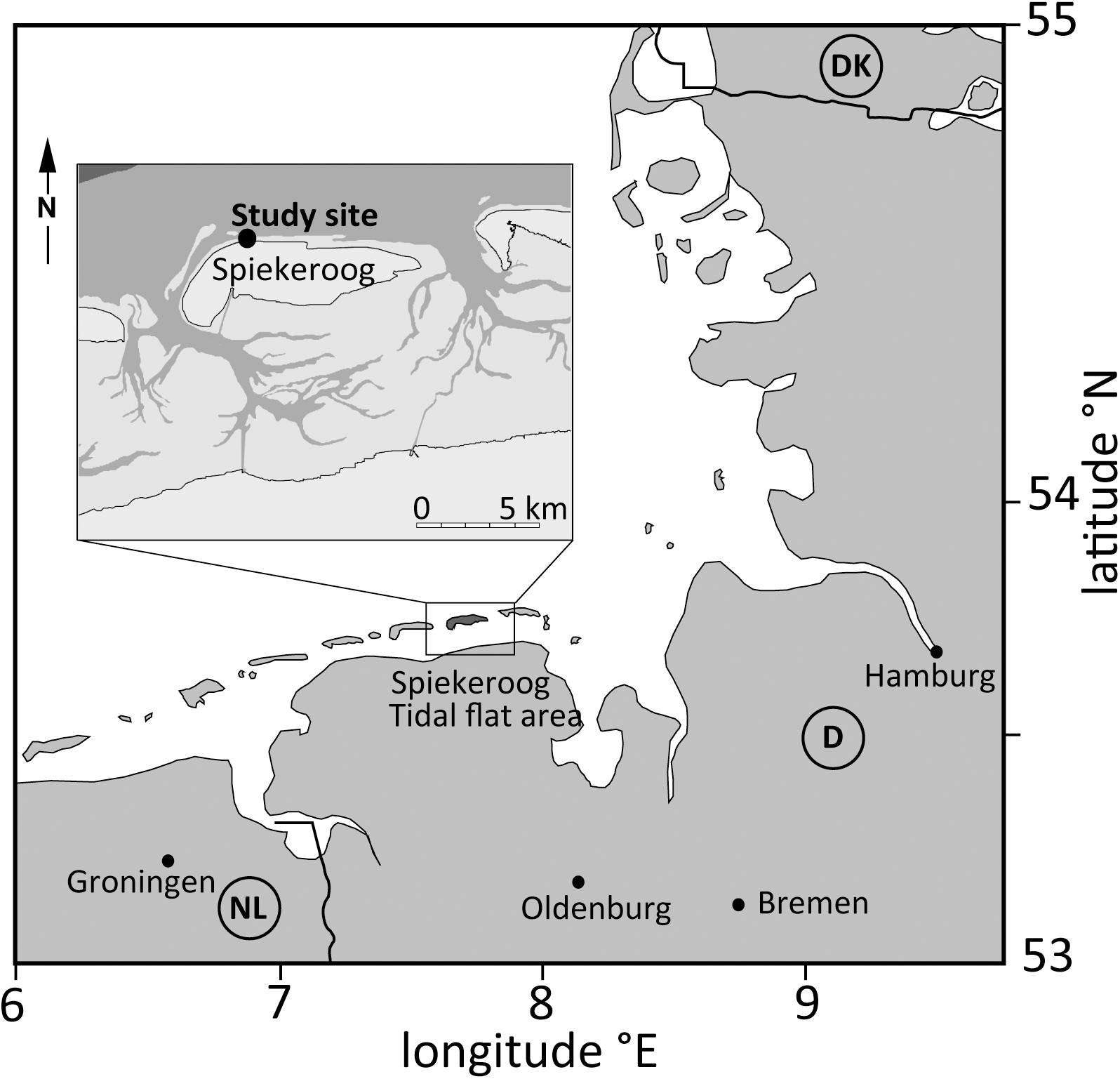
Figure 1. Sampling area on Spiekeroog Island, North Germany.

The study site along the northern shore, Spiekeroog beach, has a mean tidal range of 2.7 m, and the offshore wave heights vary from 0.5 to 2.0 m under fair weather conditions and up to 8 m during storm events (Dobrynin et al., 2010). Both wave and tidal regime generate a ridge-and-runnel system parallel to the shoreline (Anthony et al., 2005) with the most landward runnel and the following ridge located between the high and low water lines. The beach morphology changes from a dissipative state, with a less pronounced ridge-runnel relief, in the winter storm period (October–March), to a reflective stage, with a stronger ridge-runnel relief, under calm summer (April–September) conditions (Dobrynin et al., 2010).

The sedimentology and hydrology of the investigated beach site has been characterized and fed into a numerical model in Beck et al. (2017). Briefly, the beach sediments consist of quarzitic fine to medium grained sands (∼200–300 μm diameter) with occasionally distinct layers of shell debris and mud pebbles. The numerical model of Spiekeroog beach predicted the occurrence of an upper saline plume (USP), which is formed by seawater infiltration at the high water line, and which exfiltrates primarily in the runnel. Its vertical extent was calculated to reach depths of > 20 m. Phase-averaged pore water velocities at the high water line entry points were calculated to reach approximately 0.3 – 0.7 m d⁻¹. According to the model, the USP compresses the fresh discharging groundwater to a narrow fresh water discharge tube (FDT) which exclusively exfiltrates in the runnel area (Beck et al., 2017). In addition, seawater infiltration was predicted to occur on the ridge, with subsequent exfiltration in the runnel and at the low water line. The model yielded a fresh water flux of 0.75 m³ d⁻¹ m⁻¹ shoreline and a seawater flux from USP and ridge of 2.8 and 1.5 m³ d⁻¹ m⁻¹ shoreline, respectively. It has been hypothesized that efflux of nutrients from these exfiltration sites could be utilized by local microphytobenthos and phytoplankton, and subsequently, produce locally specific macrobenthic communities (Beck et al., 2017; Kröncke et al., 2018).

Sampling Strategy

Sampling took place in October 2016 (onset of winter storm season), March 2017 (end of winter storm season), and August 2017 (summer calm season). The campaigns in October and August were conducted during spring tide and the campaign in March during neap tide. Topography and pore water chemistry data were collected on 200 m × 200 m grids between the current high water line and the low water line. The two anchor points at the high water line were always the same in all three campaigns. In October and August, sampling commenced at high tide and followed the falling water, while in March sampling started at the low tide line and finished at the high water line. The location of the entire grid was chosen, because the groundwater flow gradient is relatively high due to the short distance to the dunes with a relatively clear North-South flow direction, and it is in an area away from the main tourist beach. The maximum dimension of 200 m × 200 m was allowed to complete the sampling of the full grid within one tidal cycle. Topographic data were logged on a differential GPS (Stonex S9 III Plus GNSS), at 20 m × 20 m resolution within the grid. Pore water chemistry samples were collected at two depth levels, 50 and 100 cm, below the sediment surface. The pore water samples were obtained by driving stainless steel push-point sampling lancets into the sediment, and extracting water with polyethylene (PE) syringes. Prior to sample collection, lancets and syringes were flushed with several (3–4) syringe volumes.

As proxies for STE hydrology (i.e., water residence times, infiltration and exfiltration locations), temperature and salinity were determined directly with hand-held devices (WTW Multi 3430/WTW pH/Cond 340i with TetraCon 925 Conductivity Sensors). The sensors were calibrated prior to use, using 0.01 mol/l KCl WTW conductivity standards and were checked for trueness using an OSIL Atlantic Seawater Conductivity Standard.

To track redox conditions, dissolved oxygen concentrations were measured with pre-calibrated pocket oxygen meters with a flow-cell (FireStingGO₂, Pyro-Science) during the March and August campaigns. In order to avoid bubbles, pore water was carefully extracted using PE syringes. The measurement was performed instantly using flow-through cells with an attached temperature sensor. A 2-point calibration was done 1 day prior to field measurements using air saturated seawater and a 0% calibration standard. The latter was prepared mixing seawater with a strong reductant (sodium dithionite at concentration of about 30 g/l). According to the manufacturer the instrument accuracy yields at ±1% air saturation at high dissolved oxygen concentrations and ±0.1% air saturation at low dissolved oxygen concentrations. Due to the potential unconformity of a bubble-free sampling, the assumption of an uncertainty of 2–3% air saturation would be more appropriate.

For the spectrophotometric measurement of Fe(II), 0.2 μm-filtered (Whatman Acrodisc GHP) 1 mL aliquots were fixed in 100 μL ferrozine solution. The protocol followed the method described in Viollier et al. (2000), with two adaptations, namely, the calibration reagents (0 – 200 μM) were prepared in de-aerated water using Fe(II)Cl₂, and Fe(III) was not separately determined in an additional reduction step. Measurements were conducted using microtiter plates and a spectrophotometric reader located in the laboratories of the Microbiogeochemistry group of the ICBM. Due to the high Fe(II) concentrations and the absence of a reduction step, a trace metal clean laboratory was not required for the analyses. The precision of the Fe(II) measurements was better than 5%.

Total humic-like fluorescence, a fraction of FDOM with an excitation wavelength of 350 nm and an emission wavelength of > 420 nm, was determined on 0.2 μm-filtered subsamples with a hand-held fluorometer (AquaFluor, Turner Instruments). This fraction corresponds to the terrestrial, humic-like “peak-C” DOM as described in Coble (1996). Calibration of the fluorometer was conducted using quinine sulfate solutions, in 0.05 M H₂SO₄, in the range of 50–1000 ppb. The instrument accuracy is better than 10%. In the August 2017 campaign, we collected small-volume (2 mL) 0.2 μm-filtered subsamples for dissolved silicate (DSi) analyses. The samples were analyzed spectrophotometrically (Grasshoff et al., 1999). Precision and accuracy of the method was better than 10%.

Salinity and temperature are assumed to be influenced exclusively by abiotic factors, while oxygen, Fe(II), FDOM, and DSi concentrations are proxies which may be affected by both, abiotic and biotic factors.

To characterize the subsurface flow conditions, hydraulic heads were continuously recorded with pressure transducers for a duration of 1.5 days at 5 shallow groundwater monitoring wells (filter screen from 0.5 m to 1.0 m below the ground surface) along a cross-shore profile in August. The data was corrected for the barometric pressure. In the October and March campaigns, hydraulic head data was only incompletely recorded and did not allow the deduction of groundwater flow directions.

Data Processing

Topographic and physico-chemical data were assembled together in 3D gridded maps (GMT5, Wessel et al., 2011, using the “surface” algorithm by Smith and Wessel, 1990) to identify spatial and temporal patterns. Thereafter, the relationships between topographical data and geochemical distribution patterns were explored and plotted in R (version 3.4.0, RStudio version 1.0.143) using Spearman rank tests of the package corrplot. To test for physico-chemical zonation patterns in the STE, a Principle Coordinate Analysis (PCoA) was conducted with the environmental variables temperature, salinity, and concentrations of Fe(II), FDOM, and oxygen. The values were normalized and Hellinger transformed, and the PCoA distance matrix was calculated using Bray-Curtis dissimilarities. The PCoA scores of the physico-chemical parameters were then correlated to the three topographic parameters “Elevation” (i.e., beach height), “North,” and “East.” As the beach slopes from South to North, the parameter “North” is a proxy for the land-sea gradient (i.e., cross-shore), whereas the parameter “East” is a proxy for lateral heterogeneity (i.e., parallel-shore). We color-coded different zones presumed as “infiltration” or “exfiltration” areas, to test whether specific physico-chemical zones were aligned with specific flow paths.

To evaluate the impact of different endmember choices on the constituent export from the STE, we calculated Fe(II) and FDOM fluxes based the hydrological model from Beck et al. (2017). Fluxes were calculated separately for each campaign and the two sampled depths (50 and 100 cm). Our calculations followed two main approaches. In the first approach, 10 × 10, 5 × 20, 2 × 40, 1 × 80, and 1 × 100 data points were randomly selected over the whole grid, and averaged Fe(II) and FDOM concentrations from these points were multiplied with total modeled SGD volumes (5 m³ d⁻¹ m⁻¹ shoreline). In the second approach, discharge volumes of three exfiltration sites were defined based on the runnel-ridge topography, namely for the upper runnel slope (i.e., zone from deepest runnel point to mid-way of toward the high water line, 3.15 m³ d⁻¹ m⁻¹), for the lower runnel slope (i.e., zone from the deepest runnel point to mid-way of the seaward ridge, 0.85 m³ d⁻¹ m⁻¹), and for the low water line, starting mid-way downslope from the ridge (1 m³ d⁻¹ m⁻¹). For this three-compartment-flux model, all Fe(II) and FDOM data collected in the defined areas were averaged, multiplied with the respective discharge volumes, and added up. We acknowledge that the calculated fluxes not factor in concentration changes in the shallower sediment layers (<50 cm), which will affect Fe(II) in particular (Rocha, 2008).

Results

Topography and Hydraulics of Spiekeroog Beach

The 2D beach topography confirmed a distinct runnel-ridge system as previously observed by single-line transect approaches (Anthony et al., 2005; Beck et al., 2017). The general features in the intertidal zone remained similar over the three sampling campaigns: a runnel located approximately 50 m (October and March) to 70 m (August) seaward from the high water line, a ridge with its maximum height approximately at 100 m away from the high tide line, and a ridge slope at the low water line, approximately 180 m from the high water line (Figure 2). In October, the ridge was disrupted on the eastern border of the grid by a tidal drainage channel. This tidal channel had disappeared in March, and a less pronounced channel developed toward the west. In August, a similar tidal channel as in the October campaign started to re-appear, and the slope between high water line and runnel was interrupted by several round-shaped indentations in the east (Figure 2). The maximum differences between high water line elevation and low water line elevation over the lateral distance of 200 m amounted to 3.3, 2.6, and 3.9 m in October, March, and August, respectively. The coefficients of variation (percentages of standard deviations from the mean) for beach heights were calculated to be 21, 15, and 24% in October, March, and August, respectively. Therefore, both beach gradient and beach topography heterogeneity increased in the three campaigns in the order March < October < August.

FIGURE 2

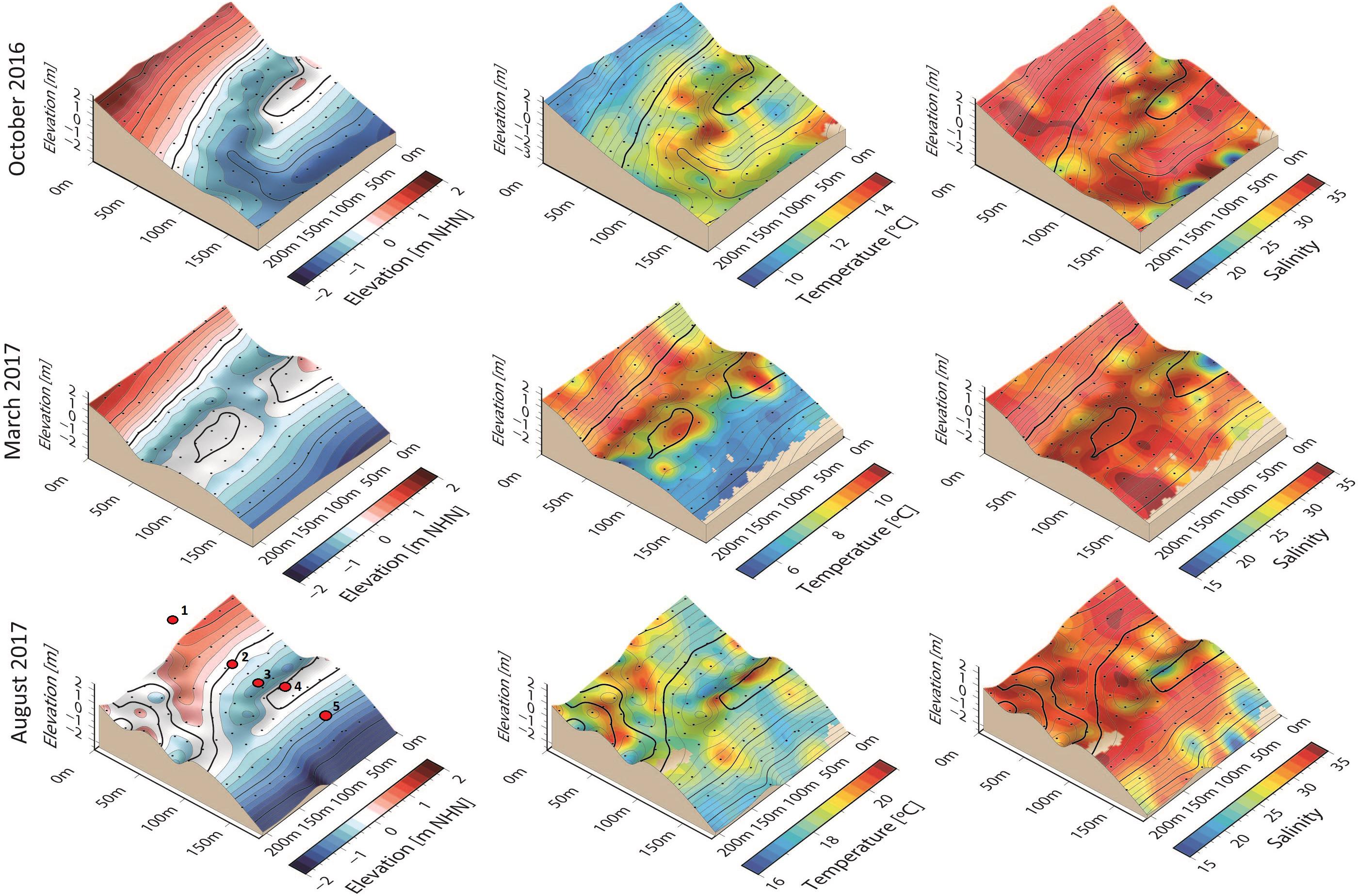
Figure 2. Beach topography and physico-chemical parameters (for sampling depth 50 cm) of Spiekeroog beach for the three sampling campaigns. The thick black lines indicate the 0 m NHN line. The highest and lowest sampling locations indicate the approximate locations of the high and low water line, respectively. Note that the temperature scale varies for the three campaigns. The red points numbered as 1–5 indicate the locations of the shallow groundwater monitoring wells GWM1 to GWM5 placed during the August 2017 campaign.

The hydraulic head signals of the 5 shallow groundwater monitoring wells in the intertidal zone were strongly influenced by the tides and the actual topographic elevation (Figure 3). Tide-averaged hydraulic heads corresponded to the topography (Figure 3), confirming the model results of Beck et al. (2017): hydraulic gradient, and thus groundwater flow were directed from both the high water line and the ridge toward the runnel, and from the ridge toward the low water line (Figure 3). This suggests seawater infiltration at the high water line and the ridge, and exfiltration in the runnel and at the low water line. The inland hydraulic head at the groundwater divide on the island typically changes on average from about 2 m asl at the end of winter to about 1.3 m asl at the end of summer, while the average hydraulic head at the high water line is rather constant with about 1m. The estimated annually averaged freshwater flux into the intertidal zone is roughly 0.75 m³/d/m (see Beck et al., 2017). This means the freshwater flux could well vary between 0.35 and 1.2 m³/d/m within the cycle of the year. The model estimated average tidally driven recirculated seawater flux is about 4.3 m³/d/m (Beck et al., 2017). This means the fraction of freshwater in the intertidal system may range between less than 10 and 30% (under the assumption that the recirculating seawater flux is constant).

FIGURE 3

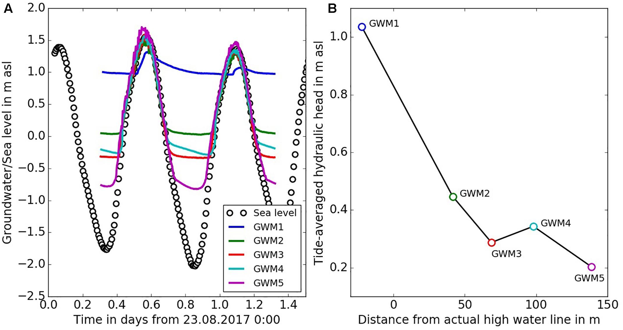
Figure 3. Hydraulic head data measured during the August 2017 campaign, (A) measured time series of hydraulic heads at monitoring wells GWM1 – GWM5 and the actual sea water level, (B) corresponding tide-averaged hydraulic heads at monitoring wells GWM1 – GWM5 along the cross-shore profile indicated in Figure 2.

Physico-Chemistry in the Shallow STE of Spiekeroog Beach

Pore water temperature was lowest in March, followed by October and August (Figure 2 and Supplementary Figure S1). There was almost no overlap between the temperature regimes of the three campaigns and clear seasonal variations were apparent. Pore water temperatures at the high water line (∼10–11°C, ∼8–10°C, and ∼18–20°C in October, March, and August, respectively) were similar to those measured in the nearshore ocean during the sampling campaigns (9.9°C, 7.5°C, and 18.5°C, respectively). On the other hand, pore water temperatures at the low water line (∼11–14°C, ∼6–7°C, and ∼17–19°C in October, March, and August) were either slightly higher (October) or slightly lower (March and August) compared to those of the nearshore ocean. By contrast, salinity ranges, oxygen saturations, and concentrations of Fe(II) and FDOM (in ppb quinine sulfate equivalents, QSE) were overall in similar ranges between sampling events, with cross-shore gradients generally dominating over seasonal changes (Figure 4 and Supplementary Figure S2). All physico-chemical parameters showed significant positive correlations between 50 cm and 100 cm depth (Spearman’s rank test, p < 0.001), confirming an overall positive co-variance of distribution patterns within the measured depth range of the shallow STE (Supplementary Figure S3).

FIGURE 4

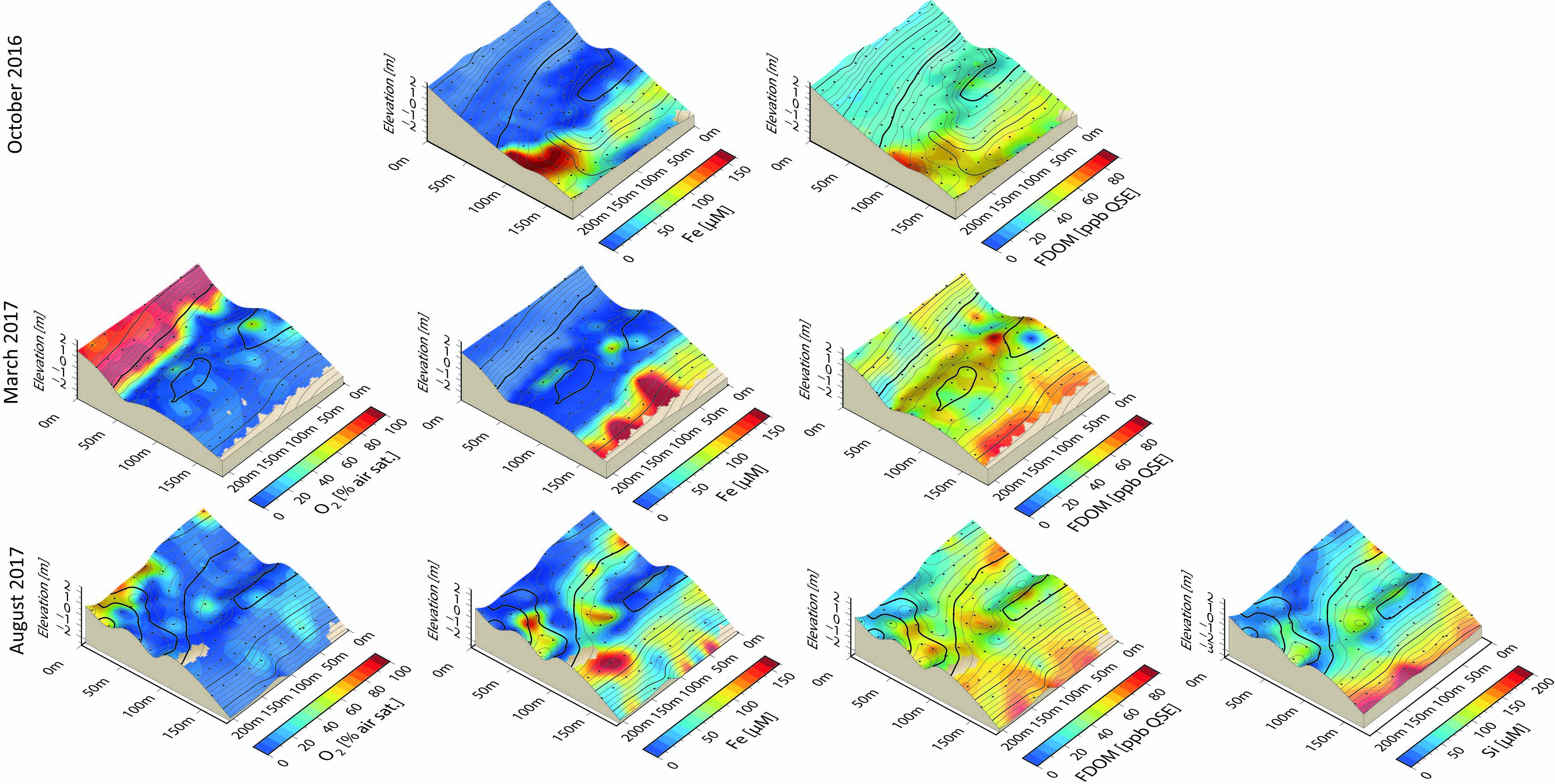
Figure 4. Biogeochemical parameters (for sampling depth 50 cm) of Spiekeroog beach for the three sampling campaigns. The highest and lowest sampling locations indicate the approximate locations of the high and low water line, respectively.

Visualization of the physico-chemical parameters on a 3D-topographical grid revealed large spatial heterogeneities, with strong parallel and cross-shore gradients, throughout all three campaigns (Figures 2, 4). In summary, these heterogeneities corresponded to visually pronounced physico-chemical zones: Temperatures showed a strong increasing (October) or decreasing (March) cross-shore gradient from high to low water line. Salinity minima occurred in the runnel and at the low water line, in particular in the October and August campaigns, with few spots additionally occurring on the ridge in the March campaign. Detailed profiling onsite revealed that these low-salinity patches were limited to approximately 1–2 m² areas. Oxygen levels measured in March and August were high at the high water line and decreased rapidly toward the runnel. Fe(II) concentrations increased strongly from the seaward slope of the ridge toward the low water line. Analogous to Fe(II), FDOM and DSi concentrations were enriched at the seaward slope of the ridge in comparison to more landward locations. Some seasonal deviations from these overall patterns were observed, notably patches of high Fe(II) concentrations between high water line and runnel in August, and elevated FDOM concentrations in the runnel in March and August, but not in October (Figure 4).

Constituent Flux Estimates: Fe(II) and FDOM

Calculated Fe(II) fluxes displayed large fluctuations when using 10 or 20 random points, and showed more stable ranges from 40 points upward, and approached the values yielded by the zone-specific approach (Supplementary Figures S4, S5). Using > 40 random points or the zone-specific approach, Fe(II) fluxes ranged between ∼100–300 mM d⁻¹ m⁻¹ shoreline, and increased in the order March < October < August. Zone-specific contributions, as well as their calculated uncertainties, varied between the three campaigns. The zone-specific uncertainties were higher overall for the two runnel sections compared to the low water line. Compared with Fe(II), calculated FDOM fluxes displayed less fluctuations using random and zone-specific approaches, and increased in the order October < March < August. From > 40 random points upward, FDOM fluxes ranged between ∼180–260 ppm QSE d⁻¹ m⁻¹ shoreline. Zone-specific contributions were generally similar over the three campaigns, and zone-specific uncertainties were again lowest for the low water line sections (Supplementary Figures S4, S5).

Discussion

Salinity Distribution, Inferred Groundwater Flow and Heat Transport Patterns

Low-salinity (<20) patches were found in the runnel and at the low water line in all campaigns. While the cross-shore distribution of these patches is clearly a function of corresponding beach topography, there seems to be no apparent link between small-scale topography variations and occurrence of the patches parallel to the shoreline. To the best of our knowledge, only one study has previously investigated lateral patchiness of fresh SGD, albeit on smaller scales (20 m × 100 m, 1–5 m spacings). On microtidal Cape Henlopen, Delaware, Dale and Miller (2007) found fresh groundwater discharge spots with distinct temperature and salinity signatures, and attributed their occurrence to buried tidal creeks underlying the homogenous fine-grained sandy beach sediments. At Spiekeroog beach, similar meso-scale heterogeneities, for example embedded layers of mud pebbles, marsh peat, or shell debris (Streif, 2002; Beck et al., 2017) could be responsible for the discontinuous discharge patterns of brackish groundwater parallel to the shoreline. An additional driver of pore water heterogeneity may be heterogeneous flow fields due to sediment sorting. In general, sediments subjected to high wave energies have an overall coarser size distribution compared to those in more sheltered areas (McLaren and Bowles, 1985). Previous sediment cores from the beach showed zig-zag like vertical variations in sediment grain size between 200 and 300 μm (Beck et al., 2017), perhaps due to repeated sediment re-suspension and settlement in this dynamic intertidal zone. Therefore, pore water flow may accelerate or slow down, depending on the local vertical stratigraphy (Rocha, 2008). Recently, alongshore movement of saline water parcels was reported in the vicinity of tidal creeks (Zhang et al., 2016). Such creeks (or tidal channels) occur on Spiekeroog beach as well, albeit with life spans in the order of days. The intrusion of seawater along creek banks could nevertheless interrupt cross-shore discharge of brackish pore water from FDT and USP.

It should be noted that the locations of the brackish pore water exit points were roughly in the same areas in October and August, pointing to somewhat consistent discharge zones for the fresh groundwater endmember. In March, we could not access the lowest points of the low water line due to the neap tide regime and onshore winds. Therefore, the absences of low-salinity patches may have been due to a limited coverage of the low water line, together with a weaker hydraulic gradient (neap tides) in this campaign compared to the other two. Rain could theoretically explain the observed brackish patches in the entire intertidal area. We do not have any data from Spiekeroog Island, but a weather station from the nearby island Norderney recorded a total precipitation of 0.6, 31, and 3 mm during the sampling campaign weeks for October, March, and August, respectively. Thus, rain could only explain the occurrence of brackish water observed in March, but not for October and August. Even then, in this case we would expect a superficial low salinity layer spread homogenously over the entire grid, rather distinct localized patches that are visible also in 100 cm depth. While the low salinity patches in the exfiltration zones were most likely attributed to groundwater originating from the freshwater lens, the reasons for them occurring on the ridge, i.e., where seawater infiltrates, are not yet clear. For one, they could be a result of density-induced salt-fingering flow squeezing fresher water upward (e.g., Greskowiak, 2014; Röper et al., 2015). Low-salinity patches may also be the remains of past fresh groundwater exfiltration, for example where a low topography point in the form of a tidal channel or runnel had been in the previous weeks. This would mean that the advective flow in the runnel-ridge area of our study site resembles less a continuous conveyor belt, and more a stop-and-go traffic (or perhaps even be subject to reversed flow) determined by the locally changing hydraulic head.

The presence of the ridge and runnel structure with its characteristic topography (more or less well developed in the different seasons) determined the tide-average hydraulic gradients and lead to principle areas of in- and exfiltration (Figures 3, 5, 6): Infiltration area 1 at the upper tidal zone and exfiltration area 1 at the landward slope of the runnel, infiltration area 2 at the top of the ridge, exfiltration area 2 and 3 at the land and sea facing flanks of the ridge near the runnel and the low water line, respectively. Previous groundwater flow and transport modeling efforts at this site (Beck et al., 2017) suggested high infiltration rates at the high water line and residence times in the USP of up to several months. Infiltration rates on the ridge were predicted to be lower, and residence times to both the runnel and low water line were calculated to be up to several years. In addition, the model of Beck et al. (2017) suggested that all freshwater from the fresh water lens discharges in the runnel, i.e., no further freshwater flow occurs below the ridge toward the low water line. Contrastingly, our new findings indicate two exfiltration areas for brackish groundwater, one in the runnel and one around the low water line. Note that the Beck et al. (2017) model slightly overestimated the measured tide-averaged hydraulic head at the top of the ridge by 0.2 m (Supplementary Figure S2 of supporting information in Beck et al., 2017), which produced a groundwater divide on the ridge and thus prevented fresh groundwater discharge at the low water line. Nevertheless, the discrepancies between the previous model and our new data imply that even small (potentially cm-scale) changes in intertidal topography, such as ridge height and location, could produce large diversions of groundwater flow paths.

FIGURE 5

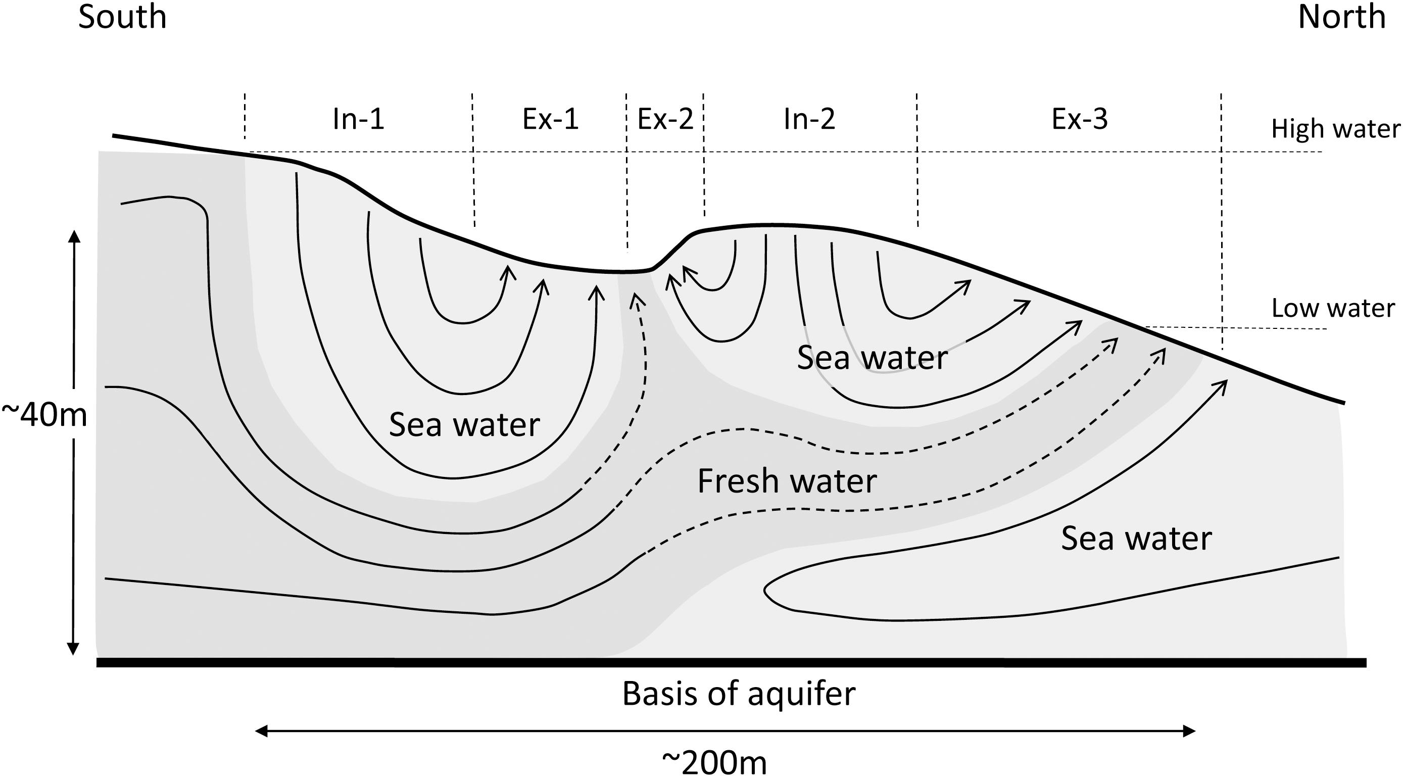
Figure 5. Conceptual model of principal cross-sectional groundwater flow field and location of in- and exfiltration areas (In-1 and In-2 indicate infiltration areas 1 and 2, respectively; Ex-1, Ex-2, and Ex-3 indicate exfiltration areas 1, 2, and 3, respectively) in the intertidal zone at the north beach of Spiekeroog.

FIGURE 6

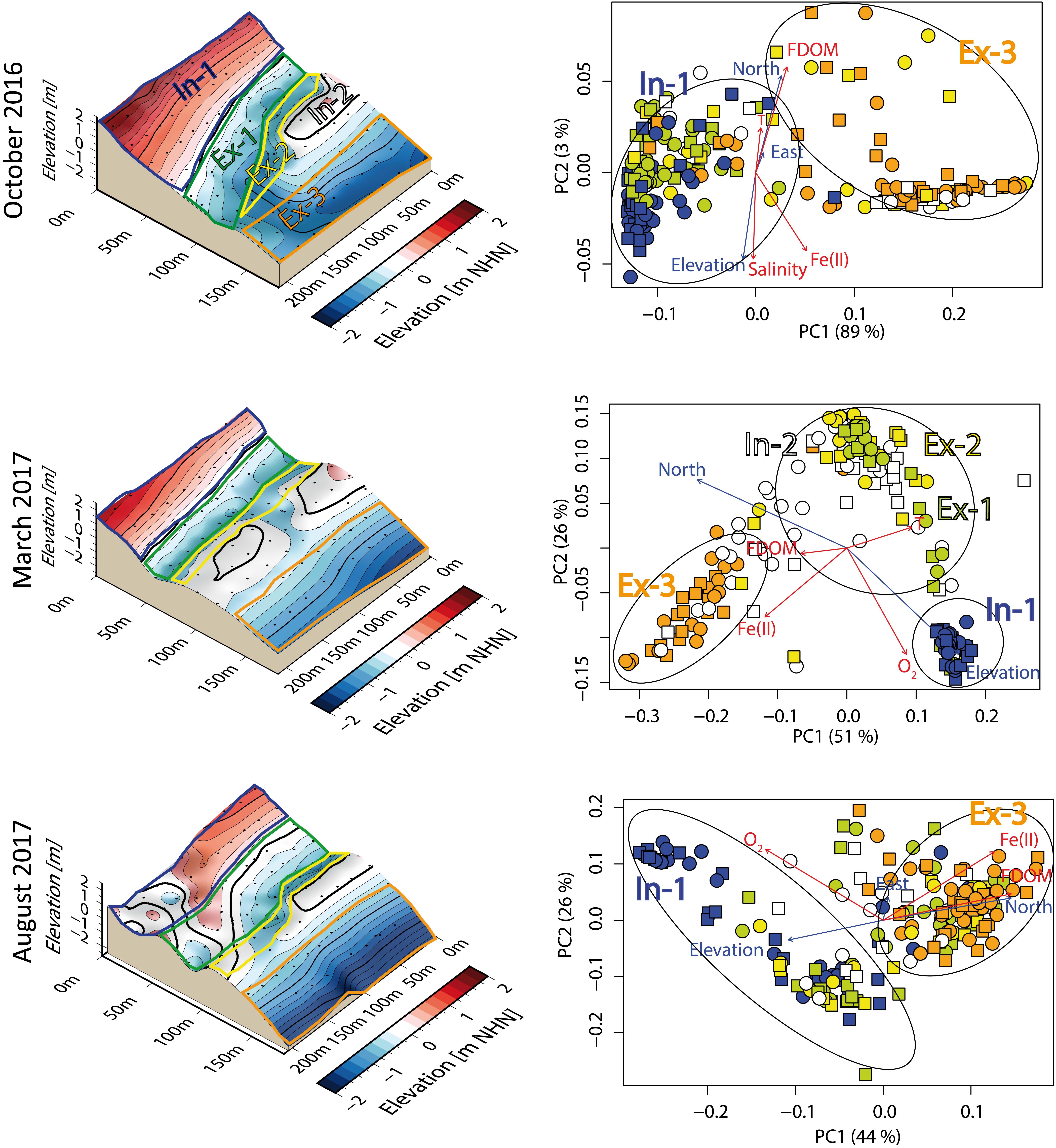
Figure 6. Principal component analysis (PCoA) for the 3 sampling campaigns in October 2016, March, 2017, and August 2017. Right panel: Only topographic and physico-chemical parameters are displayed which have a significant influence (p < 0.05) on the sample distribution in the PCoA. The ellipses in the PCoA demonstrate the clustering of different in- and exfiltration zones based on their physico-chemistry. The circles indicate data from 50 cm depth and the squares indicate data from 100 cm depth.

The pore water temperatures at the high water line were similar to those of the nearshore North Sea and confirmed infiltration of ambient seawater. On the other hand, recirculating and exfiltrating seawater appeared to carry the temperature signature of the previous months. The strong temperature decrease at the low water line compared to the high water line in March may have been induced by the exfiltration of cold seawater from the preceding winter. In August, i.e., mid-summer, the temperatures at the low water line were still slightly lower than at the high water line, suggesting discharge water that infiltrated at the end of spring/early summer. In October (i.e., fall), elevated temperatures at the low water line compared to the high water line likely reflected exfiltration of seawater from the previous, warmer summer months. These interpretations seem contrasting to the model from Beck et al. (2017), which predicted that infiltrating seawater flowing from the ridge takes up to several years to exfiltrate at the low water line. Overall, this could indicate that the residence times in USP and ridge- to low water line recirculation cell may be at the low end of the timescale ranges (weeks-months) predicted by the previous model (months-years). Furthermore, in March, pore water from both high water line (infiltration zone) and runnel (exfiltration zone) had similar temperatures which were higher than those at the low water line (Figure 2). External seasonal factors, for example solar radiation or seawater inundation, could also influence shallow STE temperature over smaller time scales (days-weeks), and overprint signals from deeper, older SGD sources. Such overprints have to be taken into account when comparing pore water temperatures with modeled water residence times, or using temperature anomalies to detect SGD via airborne thermal infrared remote sensing (Tamborski et al., 2015).

Biogeochemical Patterns

In our study, dissolved oxygen was elevated only in infiltration area 1 (In-1), and was lowest in the exfiltration areas (i.e., <10% air saturation). In infiltration area 2 (In-2), i.e., the top of the ridge, oxygen saturation levels in 50 cm and 100 cm depths were already very low, presumably because seawater infiltrates more slowly in this area, compared to In-1 (Beck et al., 2017). The decrease of oxygen concentrations was more pronounced in the August campaign compared to that in March. Considering the large (up to fourfold) differences in pore water temperatures between those two campaigns, it is likely that, in addition to the overall lower solubility of O₂ in the warmer seawater, the microbial respiration rates, and subsequent biogeochemical transformations of nutrients, iron, and DOM substantially accelerated during the summer season (O’Connor et al., 2018). There were slight operational differences between the March and August sampling campaigns; namely, sampling from low to high water in March and sampling from high to low water in August. As a result, in March, the intertidal zone was exposed to the atmosphere longer, and in August, it was exposed to seawater inundation longer. Practically, we lost the highest line of sampling data in the March campaign, as the high water line was already quite de-saturated (Figure 4). On the other hand, we did not observe an impact of atmospheric oxygen exposition or oxygenated seawater infiltration below the high water line for both campaigns. This would indicate that at the investigated depths of 50 and 100 cm, the different sampling conditions did not impact the physico-chemical conditions as much as, for example, the strong seasonal differences (mostly temperature). Our oxygen distribution patterns at high water line (In-1) and ridge (In-2) were in good agreement with corresponding sites in Beck et al. (2017) from the same beach during an earlier campaign (May 2014), displaying greater oxygen penetration depths at the former compared to the latter infiltration site. Similarly, Charbonnier et al. (2013) found successive oxygen depletion in pore waters along a cross-shore gradient on meso- to macrotidal Truc Vert beach at the French Atlantic coast. There, the oxygen gradient was interrupted during one campaign by seawater infiltration at a newly formed downstream ridge. Such a pattern could not be observed in our study, probably because Charbonnier et al. (2013) sampled the most surficial pore waters at each station, while we sampled deeper pore water, well in the saturated zone. However, Beck et al. (2017) indeed found 60 – 100% oxygen saturation in pore water from the top 5 cm of the ridge (corresponding to In-2 of our study) in May 2014. It should be noted that another study on a mesotidal beach at the Portugese Atlantic coast, reported high oxygen levels (>50%) even in the lowest exfiltration zone, which they attributed to an interplay of strong tidal oscillations, rapid advection, and low organic matter supply (Ibanhez and Rocha, 2016). In our study, we did observe some patches with relatively elevated oxygen values in the ridge-runnel area (light blue spots in Figure 4), but they always remained well below 50%. Therefore, in our study, the cross-shore oxygen consumption overall prevailed over any vertically-induced turbidities.

High levels of Fe(II) in exfiltration area 3 (Ex-3) were consistent across the three sampling campaigns. Dissimilatory iron reduction is a common microbial process in STEs and follows the succession of oxygen, nitrate, and manganese oxide respiration when water residence times increase (Froelich et al., 1979). Iron(III) reduction relies on the provision of electron donors, mostly in the form of fresh marine organic matter during seawater infiltration (Snyder et al., 2004; Roy et al., 2010; Reckhardt et al., 2015; Beck et al., 2017). Although sulfide concentrations were below detection limit, sulfide smells were noted in some samples and the sediment exhibited grayish layers indicating the presence of iron sulfides. These observations indicate that sulfate reduction occurred simultaneously with or in the vicinity of Fe(III) reduction in the very old pore waters of the low water line. In addition, Fe(II) concentrations were very low in low-salinity patches compared to high-salinity areas at the low water line, probably because the fresh groundwater component was more depleted in Fe(II) compared to the exfiltrating seawater from the ridge. These results are in line with Seibert et al. (2018), who attributed the absence of Fe(II) in the older groundwater of the island’s freshwater lens to the formation of iron sulfides in succession to sulfate reduction.

Compared to the low water line, exfiltrating pore water in the runnel (Ex-1 and Ex-2) was overall more depleted in Fe(II). In general, advective flow paths from the high water line to the runnel should have shorter residence times compared to those from the ridge to the low water line (as modeled in Beck et al., 2017), and therefore pore water likely discharged before commencement of (substantial) iron reduction. However, in August, patches of elevated Fe(II) concentrations were found between high water line and runnel, while Fe(II) concentrations close to the low water line were overall lower compared to the other sampling campaigns. Phytoplankton blooms in the southern North Sea commonly start in March–April and undergo several successions throughout the summer and fall (June–October, Speeckaert et al., 2018). The combination of marine-derived electron donor surplus and overall high temperatures during the summer months probably accelerated microbial respiration rates. Subsequently, an enrichment of Fe(II) in exfiltrating, “younger” pore water at the runnel (Ex-1 and Ex-2) due to elevated iron reduction, and a depletion of Fe(II) in exfiltrating, “older” pore water at the low water line (Ex-3) due to elevated sulfate reduction, was evident in the August campaign compared to the other seasons.

The co-occurrences of FDOM maxima with low salinity patches were likely connected to the characteristics of the measured fluorescence: the hand-held fluorometer used in this study targets terrestrially-derived, humic-like fluorescent DOM fractions (“peak-C”, Coble, 1996) and this fluorescence signal has been used to trace land-derived DOM in SGD (Nelson et al., 2015; Kim and Kim, 2017). Most likely sources of FDOM at the study site include leachates of recent terrestrial inland vegetation, or hydrolyzed DOM from Pleistocene marsh peats (Streif, 2002). Therefore, co-occurrences of FDOM with low-salinity patches (Figure 4 and Supplementary Figure S6) do indicate that fresh groundwater transports vascular, terrestrial-plant-derived DOM into the STE, although they do not allow differentiation between recent and old vascular DOM fractions. It has also been suggested that aromatic, humic-like secondary metabolites produced by marine pro- and eukaryotes can cause peak-C fluorescence (Romera-Castillo et al., 2010, 2011). Therefore, breakdown of buried marine phytoplankton may contribute to the observed FDOM signal in the STE (Ehrenhauss et al., 2004). Furthermore, the same FDOM fraction (peak-C) was previously linked to marine organic matter degradation in a microtidal STE (Suryaputra et al., 2015). While phytoplankton per se may not contain substantial amounts of humic-like organic matter, we observed deposition and burial of macroalgae (mostly Fucus vesiculosus) along the high water line. The release of these marine-derived organic materials, together with a preferential respiration of aliphatic DOM by the STE microbial community, may have led to an increased accumulation of DOM with higher aromaticities along the STE flow paths.

Finally, FDOM in our study was also significantly positively correlated with Fe(II) concentrations. Fe(oxy)hydroxide precipitation, which commonly occurs at STE redox interfaces (“iron curtain, Charette and Sholkovitz, 2002) can scavenge aromatic, humic-like fractions of DOM, analogous to the peak-C FDOM measured in our study (Linkhorst et al., 2017). During reductive dissolution of Fe oxides, both Fe(II) and bound humic-like DOM are released again (Seidel et al., 2015; Sirois et al., 2018). Hence these specific DOM compound groups may be de-coupled from their (marine or terrestrial) source, with the iron curtain acting as a transient storage site. The coupling of Fe species and FDOM was particularly evident in the spatial co-variations of the two parameters in the August campaign (Figure 4). Little FDOM was found near the high tide line because the infiltrating seawater in that part of the beach was overall depleted in humic-like components compared to the terrestrial endmember, and because Fe(II) reduction was limited by the presence of oxygen.

DSi concentration patterns in August 2017 roughly matched those of Fe(II) and FDOM, and overall confirmed exfiltration in the runnel and at the low water line. In contrast to Fe(II) and FDOM, DSi is not affected by changing redox conditions, and not utilized by the STE microbial community. A previous study reported rapid, short-term release of biogenic, diatom-derived DSi in shallow sediment layers, and slow, long-term release of lithogenic DSi in the deep STE (Ehlert et al., 2016). Hence, the DSi concentration can be a reliable proxy for water residence times, implying that Ex-3 discharged older pore water than Ex-1 and Ex-2 during the August campaign (Figure 4).

Key Influences on the Shallow Pore Water Chemistry

The 3D grids revealed high physico-chemical heterogeneity within the shallow pore water of the intertidal zone. Longshore variability, though clearly visible, was less pronounced than the cross-shore variability; similar to what was found by Dale and Miller (2007) and Charbonnier et al. (2013). However, longshore variability was higher in October and August. This may have been caused by a tidal channel cutting into the ridge in the former and the existence of the indentation structures in the latter, both interrupting the longshore morphology. Furthermore, the presence of low-salinity areas, which showed strong longshore heterogeneity, was more pronounced in October and August compared to March. With respect to the biogeochemical patterns observed in the different campaigns, seasonal temperature differences seemed to be relevant. For instance, in March the low temperatures of the infiltrating sea water and the corresponding low microbial aerobic respiration rates seemingly caused the homogeneous alongshore presence of dissolved oxygen in In-1.

The observed patterns were also apparent in the principal component analyses (PCoA, Figure 6). While a distinct separation of the physico-chemical character between In-1, the runnel (Ex-1 + Ex-2), and the exfiltration area Ex-3 was seen in March, separation of the in- and exfiltration zones was less clear in October and August. Nevertheless, In-1 and Ex-3 showed always a contrasting character in all sampling campaigns. Further, the PCoA confirmed that the variability in the data correlated more to the cross-shore (North) rather than the longshore (East) distance, as indicated by the much longer North-vector compared to the East-vector in Figure 6. For October, hydrochemical data from In-1 and Ex-1 and partly Ex-2 plotted in the same area within the PCoA-diagram (Figure 6). This could be due to the lack of oxygen data in October, which may have resulted in a higher separation of the high water line data compared to that of the runnel. In August, the general depletion of dissolved oxygen in the entire grid likely caused a partial overlap of In-1 and runnel (Ex-1 and Ex-2). The local presence of dissolved oxygen, and the absence of FDOM and Fe(II) in In-1 therefore appeared to be the main factors in geochemically separating In-1 from Ex-1. Strong anti-correlations between dissolved oxygen and Fe(II), were also evident by the vectors in the PCoA plot which are long and orientated perpendicular to each other.

While the In-1 and Ex-3 areas were clearly identifiable by their hydrochemical character (as their data plot in separate areas in the PCoA), the areas In-2, Ex-1 and Ex, 2 were less distinct. In-2, Ex-1 and Ex-2 data were very heterogeneous, i.e., sometimes they were separated from In-1 and Ex-3, and sometimes dispersed over the entire diagram. One reason may be the less stable position and continuity of the ridge and runnel compared to the high and low water line. For instance, in October a wide tidal channel interrupted the ridge in longshore direction, while the ridge was re-established in March. Further, in August, the runnel toward the east was less pronounced due to the presence of the round-shaped indentations. This means that the continuities of the ridge and runnel structures are more affected by erosion and sedimentation processes than areas near the high and low tide water line. As a result, the physico-chemical character in the ridge (In-2) and runnel system (Ex-1, Ex-2) was more dynamic, in contrast to the more stable conditions at the high (In-1) and the low water line (Ex-3).

Furthermore, the In-1 and Ex-3 compartments were very different from each other, likely because they have different endmembers – In-1 only seawater, Ex-3 (older) recirculated seawater and fresh groundwater – and because the water residence times are strongly different (hours in In-1 vs. months–years in Ex-3) which impacts the redox state of the pore water chemistry. This would explain why the best separation was found for in March, because there microbial respiration should be slowed down the most along the flow paths, thus leading to predominantly oxic conditions in the In-1 compartment. In comparison, in October and August, increasing temperatures and water column productivities increased the reactivity of the STE, so that the different compartments were more similar in their biogeochemistry and moved closer together in the PCoA plots. There, it became difficult to distinguish the compartments based on cross-shore direction alone, with the exception of In-1 and Ex-3.

Besides the PCoA, another approach can be the utilization of vertical concentration gradients as indicators of flow path reactivity. For the August campaign, which displayed the largest biogeochemical heterogeneities, we calculated the gradient between the concentrations at 50 and 100 cm depth, as: X_gradient = $\frac{{\text{conc}}_{100\text{cm}}-{\text{conc}}_{50\text{cm}}}{0.5\text{m}}$ [where X are the biogeochemical parameters Fe(II), FDOM, and DSi], and plotted the results on the topographical grid (Figure 7). The underlying assumption was that in infiltration zones, a positive gradient would indicate increasing release of the constituent with increasing depth, while in exfiltration zones a negative gradient would indicate increasing accumulation of the constituent with decreasing depth. With this method, it was possible to visualize matching in- and exfiltration patterns in the ridge-runnel zone for all three chemical constituents (Figure 7). Increasing concentration gradients with increasing sediment depths revealed that FDOM and DSi were already released in the high water line area, demonstrating the efficient decomposition of infiltrating marine organic matter and initiation of lithogenic silica dissolution (Ehrenhauss et al., 2004; Ehlert et al., 2016). Note that in contrast to FDOM and DSi, Fe(II) gradients were not good indicators of infiltration at the high water line, probably because Fe(II) release required longer water residence times than the other two parameters. On the flow paths with intermediate residence times, namely the runnel and ridge, Fe(II) reduction commenced, with Fe(II) concentrations, together with those of FDOM and DSi, increasing from 100 to 50 cm depth in the runnel exfiltration zone (negative gradient) and increasing from 50 to 100 cm depth on the ridge infiltration zone (positive gradient). Interestingly, total Fe(II), FDOM, and DSi concentrations (Figure 4) were highest at the low water line, highlighting their strongest accumulation with the assumed highest residence times exits. However, the vertical concentration gradients approached zero for all three constituents. There, concentration gradients were perhaps influenced by a variety of other factors, for example Fe(II) removal by sulfide reduction, and reduced release of FDOM and DSi as (i) electron donor (labile organic matter) and acceptor [for example, Fe(III)] supplies were mostly exhausted, and (iii) lithogenic silica dissolution had reached thermodynamic equilibrium with the ambient solid phase (see also Ehlert et al., 2016).

FIGURE 7

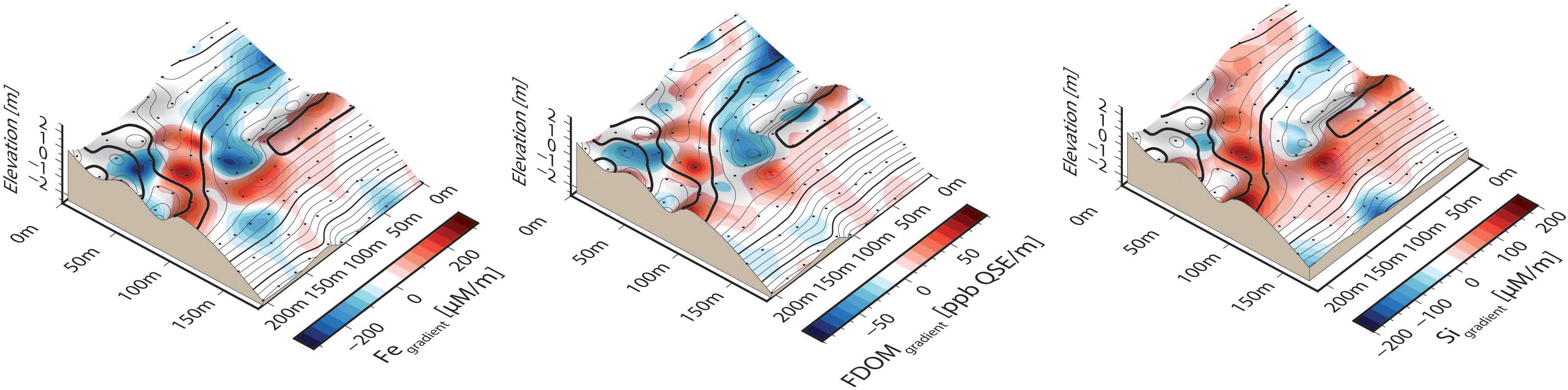
Figure 7. Concentration gradients for Fe(II), FDOM, and DSi from the August 2017 campaign. Warm colors indicate infiltration zones (conc_{100 cm}> conc_{50 cm}), cool colors indicate exfiltration zones (conc_{100 cm}< conc_{50 cm}).

Constituent Fluxes: Implications for SGD Endmember Determination

The high physico-chemical heterogeneity within the beach STE caused large uncertainties in calculated constituent fluxes. Increasing numbers of random sampling points decreased the large uncertainties, but zone-specific calculations revealed that some exfiltration areas in the STE could be more vulnerable toward heterogeneity-based biases than others (Supplementary Figures S4, S5). As expected based on previous studies, seasonal variations set the stage for microbial metabolism in terms of temperature and food regime. However, beach topography was a so far underexplored influencing factor in this mesotidal, wave-impacted study site. This factor impacts (i) exposure and immersion times to ambient air and seawater, (ii) exfiltration and infiltration patterns parallel and cross-shore in alternating ridge-runnel systems, (iii) water residence times and electron donor-acceptor supply for the sediment body as microbial bioreactor, and (iv) uncertainties in SGD constituent flux calculations. Patchy distributions of physico-chemical parameters could be produced by sediment composition heterogeneity as well as temporal changes of topography through sediment transport, causing a temporal de-coupling of physico-chemical parameters as hydraulic and metabolic processes adjust to new conditions. Choosing an inadequate exfiltration site (i.e., in the case of our study, only runnel or low water line) may severely bias SGD constituent flux calculations and increase uncertainties. Nevertheless, general spatial patterns indicate that physico-chemical parameters can reflect an approximation to steady-state conditions. In our study, the exfiltration sites with the strongest hydraulic gradients (i.e., the runnel) or longest water residence times (i.e., the low water line) were always associated with specific regimes [e.g., low Fe(II), high FDOM, low salinities vs. high Fe(II), high FDOM, low salinities]. Furthermore, microbial transformations caused consistent patterns of co-variance, for example a positive correlation between Fe(II) and FDOM, and a negative correlation between both and oxygen saturation. Therefore, zone-specific approaches were a valuable tool in identifying and comparing steady-state (low water line) and non-steady state (runnel) exfiltration sites.

Conclusion

The horizontal 2D grid sampling revealed relatively stable long-shore orientated in- and exfiltration areas in the intertidal zone of the Spiekeroog high-energy beach. Nevertheless, the in- and exfiltration areas on the ridge and in the runnel seemed to be more affected by morphodynamic changes, and therefore displayed large heterogeneities with respect to the shallow pore water chemistry. Cross-shore hydrochemical variations could largely be attributed to the in- and exfiltration areas. Though not investigated in the present study, the rather random long-shore variability could be attributed to heterogeneity of the physical properties of the aquifer material, such as hydraulic conductivity and porosity, which, in the shallow subsurface, of course are also affected by erosion and sedimentation induced changes in sediment texture. The observed variations of the pore water chemistry between sampling campaigns seemed to be largely a function of the seasonal temperature variations, although seasonal changes of the inland hydraulic head may have also played a role. The present study highlights the high temporal and spatial dynamics of pore water chemistry in the intertidal zone of a high energy beach, confirming the findings of Charbonnier et al. (2013), who investigated a high-energy beach with similar hydrological and hydrogeological conditions. Clearly, the variability in water flow paths and associated water residence times due to morphodynamic changes, especially in ridge and runnel areas, and its impact on constituent processing along the way, will add to the overall uncertainty in mass flux calculations. We argue that the calculation of a representative groundwater end-member based on random sampling to estimate SGD element fluxes in such a dynamic system is not the best option. Rather, zone-specific ranges of element concentrations should be considered for mass flux calculations, accounting for long-shore variability of the different exfiltration areas. In addition, morphodynamics may only allow for constituent flux calculations on a daily or weekly base.

Data Availability

The datasets generated for this study are available on request to the corresponding author.

Author Contributions

HW, JG, GM, SA, BE, HB, KP, OZ, and TD conceptualized the study and manuscript outlines. HW, JG, and MB wrote the main body of the manuscript. JA contributed the figures. PB, JD, NG, CE, MH, HKM, DM, BS, KS, HS, and VV edited, corrected, and extended the manuscript.

Funding

This study was financed by the Niedersächsisches Ministerium für Wissenschaft und Kultur (MWK) in the scope of project “BIME” (ZN3184) the Max Planck Society and DFG-Research Center/Cluster of Excellence “The Ocean in the Earth System” at the University of Bremen.

Conflict of Interest Statement

The authors declare that the research was conducted in the absence of any commercial or financial relationships that could be construed as a potential conflict of interest.

Acknowledgments

We are grateful to Patric Bourceau, Kai Blumberg, Lukas Brennecke, Leon Diehl, Matthias Friebe, Franziska Gluderer, Eleonore Gründken, Alina Harms, Julia Kirchner, Michael Kossack, Claas Henning Lünsdorf, Frank Meyerjürgens, Corinna Mori, Judith Otten, Janina Schulz, Niek Stortenbeker, Christoph Tholen, and Bram Vekeman for their help with 3D-grid sampling. We would also like to thank Helmo Nicolai from Terramare and Joachim Ihnken from the Niedersächsische Landesbetrieb für Wasserwirtschaft, Küsten, und Naturschutz (NLWKN) for equipment transport, and Swaantje Fock and Carsten Heithecker from the Ummweltzentrum Wittbülten for providing on-site infrastructure. Furthermore, we would like to thank the three reviewers who helped to improve the manuscript with their thoughtful comments. Finally, we are indebted to the late Dr. Gerald Millat, Dr. Gregor Scheiffarth, and Lars Scheller from the Nationalparkverwaltung Niedersächsisches Wattenmeer, for their support and cooperation in acquiring sampling permits.

Supplementary Material

The Supplementary Material for this article can be found online at: https://www.frontiersin.org/articles/10.3389/fmars.2019.00154/full#supplementary-material

FIGURE S1 | Beach topography and physico-chemical parameters (for sampling depth 100 cm) of Spiekeroog beach for the three sampling campaigns.

FIGURE S2 | Biogeochemical parameters (for sampling depth 100 cm) of Spiekeroog beach for the three sampling campaigns.

FIGURE S3 | Correlation plots (Spearman‘s rank test) of physico-chemical parameters between sampling depths 50 and 100 cm for Spiekeroog beach for the three sampling campaigns. Ellipse directions and colors depict type of correlation (positive or negative). Ellipse shapes depict strength of the correlation. Stars denote the p-value (^∗ = 0.05, ^∗∗ = 0.01, ^∗∗∗ = 0.001 significance level), numbers denote the correlation coefficient (Spearman‘s ρ).

FIGURE S4 | Flux calculations for Fe(II) and FDOM using pore water data from 50 cm depth. Left panel: definition of infiltration and exfiltration zones for the three campaigns. HWL, high water line (infiltration zone); Runnel Ex1, upper part of runnel (exfiltration zone, 3.15 m³ d⁻¹ m⁻¹ shoreline); Runnel Ex 2, lower part of runnel (exfiltration zone, 0.85 m³ d⁻¹ m⁻¹ shoreline), Ridge (infiltration zone); LWL Ex3, Low water line (exfiltration zone, 1 m³ d⁻¹ m⁻¹ shoreline). For the random approach, points were selected without regards to zonation, and multiplied with the total SGD volume (5 m³ d⁻¹ m⁻¹ shoreline). Right panel: Comparison of Fe(II) (A,C,E) and FDOM (B,D,F) fluxes calculated for October (A,B), March (C,D), and August (E,F) from random points (blue bars) and the zone-specific approach (bars in the respective colors of the exfiltration zones). Error bars denote standard errors of means. Numbers on the x axes denote sum of points used for the calculations, numbers next to the zone-specific fluxes indicate numbers of points used for each zone.

FIGURE S5 | Flux calculations for Fe(II) and FDOM using pore water data from 100 cm depth. Left panel: definition of infiltration and exfiltration zones for the three campaigns. HWL, High water line (infiltration zone); Runnel Ex1, upper part of runnel (exfiltration zone, 3.15 m³ d⁻¹ m⁻¹ shoreline); Runnel Ex 2, lower part of runnel (exfiltration zone, 0.85 m³ d⁻¹ m⁻¹ shoreline), Ridge (infiltration zone); LWL Ex3, Low water line (exfiltration zone, 1 m³ d⁻¹ m⁻¹ shoreline). For the random approach, points were selected without regards to zonation, and multiplied with the total SGD volume (5 m³ d⁻¹ m⁻¹ shoreline). Right panel: Comparison of Fe(II) (A,C,E) and FDOM (B,D,F) fluxes calculated for October (A,B), March (C,D), and August (E,F) from random points (blue bars) and the zone-specific approach (bars in the respective colors of the exfiltration zones). Error bars denote standard errors of means. Numbers on the x axes denote sum of points used for the calculations, numbers next to the zone-specific fluxes indicate numbers of points used for each zone.

FIGURE S6 | Scatter plot of FDOM concentrations vs. salinity for all three campaigns and all depths. Circles denote 50 cm depth, squares denote 100 cm depth. Fe(II) concentrations are color-coded onto the symbols, with darker colors indicating higher Fe(II) concentrations.

References

Anschutz, P., Smith, T., Mouret, A., Deborde, J., Bujan, S., Poirier, D., et al. (2009). Tidal sands as biogeochemical reactors. Estuar. Coast. Shelf Sci. 84, 84–90. doi: 10.1016/j.ecss.2009.06.015

CrossRef Full Text | Google Scholar

Anthony, E. J., Levoy, F., Monfort, O., and Degryse-Kulkarni, C. (2005). Short-term intertidal bar mobility on a ridge-and-runnel beach, Merlimont, northern France. Earth Surf. Process. Landf. 30, 81–93. doi: 10.1002/esp.1129

CrossRef Full Text | Google Scholar

Beck, A. J., Cochran, J. K., and Sañudo-Wilhelmy, S. A. (2010). The distribution and speciation of dissolved trace metals in a shallow subterranean estuary. Mar. Chem. 121, 145–156. doi: 10.1016/j.marchem.2010.04.003

CrossRef Full Text | Google Scholar

Beck, M., Reckhardt, A., Amelsberg, J., Bartholomä, A., Brumsack, H. J., Cypionka, H., et al. (2017). The drivers of biogeochemistry in beach ecosystems: a cross-shore transect from the dunes to the low-water line. Mar. Chem. 190, 35–50. doi: 10.1016/j.marchem.2017.01.001

CrossRef Full Text | Google Scholar

Burnett, W. C., Bokuniewicz, H., Huettel, M., Moore, W. S., and Taniguchi, M. (2003). Groundwater and pore water inputs to the coastal zone. Biogeochemistry 66, 3–33. doi: 10.1023/B:BIOG.0000006066.21240.53

CrossRef Full Text | Google Scholar

Charbonnier, C., Anschutz, P., Poirier, D., Bujan, S., and Lecroart, P. (2013). Aerobic respiration in a high-energy sandy beach. Mar. Chem. 155, 10–21. doi: 10.1016/j.marchem.2013.05.003

CrossRef Full Text | Google Scholar

Charette, M. A., and Sholkovitz, E. R. (2002). Oxidative precipitation of groundwater-derived ferrous iron in the subterranean estuary of a coastal bay. Geophys. Res. Lett. 29, 85-1–85-4. doi: 10.1029/2001GL014512

CrossRef Full Text | Google Scholar

Charette, M. A., and Sholkovitz, E. R. (2006). Trace element cycling in a subterranean estuary: part 2. Geochemistry of the pore water. Geochim. Cosmochim. Acta 70, 811–826. doi: 10.1016/j.gca.2005.10.019

CrossRef Full Text | Google Scholar

Cho, H. M., Kim, G., Kwon, E. Y., Moosdorf, N., Garcia-Orellana, J., and Santos, I. R. (2018). Radium tracing nutrient inputs through submarine groundwater discharge in the global ocean. Sci. Rep. 8:2439. doi: 10.1038/s41598-018-20806-2

PubMed Abstract | CrossRef Full Text | Google Scholar

Coble, P. G. (1996). Characterization of marine and terrestrial DOM in seawater using excitation-emission matrix spectroscopy. Mar. Chem. 51, 325–346. doi: 10.1016/0304-4203(95)00062-3

CrossRef Full Text | Google Scholar

Cook, P. G., Rodellas, V., and Stieglitz, T. C. (2018). Quantifying surface water, porewater, and groundwater interactions using tracers: tracer fluxes, water fluxes, and end-member concentrations. Water Resour. Res. 54, 2452–2465. doi: 10.1002/2017WR021780

CrossRef Full Text | Google Scholar

Dale, R. K., and Miller, D. C. (2007). Spatial and temporal patterns of salinity and temperature at an intertidal groundwater seep. Estuar. Coast. Shelf Sci. 72, 283–298. doi: 10.1016/j.ecss.2006.10.024

CrossRef Full Text | Google Scholar

Dobrynin, M., Gayer, G., Pleskachevsky, A., and Guenther, H. (2010). Effect of waves and currents on the dynamics and seasonal variations of suspended particulate matter in the North Sea. J. Mar. Syst. 82, 1–20. doi: 10.1016/j.jmarsys.2010.02.012

CrossRef Full Text | Google Scholar

Ehlert, C., Reckhardt, A., Greskowiak, J., Liguori, B. T., Böning, P., Paffrath, R., et al. (2016). Transformation of silicon in a sandy beach ecosystem: insights from stable silicon isotopes from fresh and saline groundwaters. Chem. Geol. 440, 207–218. doi: 10.1016/j.chemgeo.2016.07.015

CrossRef Full Text | Google Scholar

Ehrenhauss, S., Witte, U., Janssen, F., and Huettel, M. (2004). Decomposition of diatoms and nutrients dynamics in permeable North Sea sediments. Cont. Shelf Res. 24, 721–737. doi: 10.1016/j.csr.2004.01.002

CrossRef Full Text | Google Scholar

Evans, T. B., and Wilson, A. M. (2016). Groundwater transport and the freshwater – saltwater interface below sandy beaches. J. Hydrol. 538, 563–573. doi: 10.1016/j.jhydrol.2016.04.014

CrossRef Full Text | Google Scholar

Evans, T. B., and Wilson, A. M. (2017). Submarine groundwater discharge and solute transport under a transgressive barrier island. J. Hydrol. 547, 97–110. doi: 10.1016/j.jhydrol.2017.01.028

CrossRef Full Text | Google Scholar

Flemming, B. W. (2005). “Tidal environments,” in Encyclopedia of Coastal Science, ed. M. Schwartz (Berlin: Springer), 1180–1185.

Google Scholar

Flemming, B. W. (2012). “Siliciclastic Back-Barrier Tidal Flats,” in Principles of Tidal Sedimentology, eds R. A. Davies and R. W. Dalrymple (Berlin: Springer), 231–267. doi: 10.1007/978-94-007-0123-6_10

CrossRef Full Text | Google Scholar

Froelich, P. N., Klinkhammer, G. P., Bender, M. L., Luedtke, N. A., Heath, G. R., Cullen, D., et al. (1979). Early oxidation of organic matter in pelagic sediments of the eastern equatorial Atlantic: suboxic diagenesis. Geochim. Cosmochim. Acta 43, 1075–1090. doi: 10.1016/0016-7037(79)90095-4

CrossRef Full Text | Google Scholar

Grasshoff, K., Kremling, K., and Erhardt, M. (1999). Methods of Seawater Analysis. Weinheim: Wiley-VCH. doi: 10.1002/9783527613984

CrossRef Full Text | Google Scholar

Greskowiak, J. (2014). Tide-induced salt-fingering flow during submarine groundwater discharge. Geophys. Res. Lett. 41, 6413–6419. doi: 10.1002/2014GL061184

CrossRef Full Text | Google Scholar

Ibanhez, J. S. P., and Rocha, C. (2016). oxygen transport and reactivity within a sandy seepage face in a mesotidal lagoon (Ria Formosa, Southwestern Iberia). Limnol. Oceanogr. 61, 61–77. doi: 10.1002/lno.10199

CrossRef Full Text | Google Scholar

Kim, J., and Kim, G. (2017). Inputs of humic fluorescent dissolved organic matter via submarine groundwater discharge to coastal waters off a volcanic island (Jeju, Korea). Sci. Rep. 7:7921. doi: 10.1038/s41598-017-08518-8515

PubMed Abstract | CrossRef Full Text | Google Scholar

Kim, K. H., Heiss, J. W., Michael, H. A., Cai, W.-J., Laattoe, T., Post, V. E. A., et al. (2017). Spatial patterns of groundwater biogeochemical reactivity in an intertidal beach aquifer. J. Geophys. Res. Biogeosci. 122, 2548–2562. doi: 10.1002/2017JG003943

CrossRef Full Text | Google Scholar

Kröncke, I., Becker, L. R., Badewien, T. H., Bartholomä, A., Schulz, A.-C., and Zielinski, O. (2018). Near- and offshore macrofauna communities and their physical environment in a south-eastern north sea sandy beach system. Front. Mar. Sci. 5:497. doi: 10.3389/fmars.2018.00497

CrossRef Full Text | Google Scholar

Linkhorst, A., Dittmar, T., and Waska, H. (2017). Molecular fractionation of dissolved organic matter in a shallow subterranean estuary: the role of the iron curtain. Environ. Sci. Technol. 51, 1312–1320. doi: 10.1021/acs.est.6b03608

PubMed Abstract | CrossRef Full Text | Google Scholar

McAllister, S. M., Barnett, J. M., Heiss, J. W., Findlay, A. J., MacDonald, D. J., Dow, C. L., et al. (2015). Dynamic hydrologic and biogeochemical processes drive microbially enhanced iron and sulfur cycling within the intertidal mixing zone of a beach aquifer. Limnol. Oceanogr. 60, 329–345. doi: 10.1002/lno.10029

CrossRef Full Text | Google Scholar

McLaren, P., and Bowles, D. (1985). The effects of sediment transport on grain-size distributions. J. Sediment. Res. 55, 457–470.

Google Scholar

Miller, D. C., and Ullman, W. J. (2004). Ecological consequences of groundwater discharge to Delaware Bay, USA. Ground Water 42, 959–970. doi: 10.1111/j.1745-6584.2004.tb02635.x

CrossRef Full Text | Google Scholar

Moore, W. S. (1999). The subterranean estuary: a reaction zone of ground water and sea water. Mar. Chem. 65, 111–125. doi: 10.1016/S0304-4203(99)00014-6

PubMed Abstract | CrossRef Full Text | Google Scholar

Nelson, C. E., Donahue, M. J., Dulaiova, H., Goldberg, S. J., La Valle, F. F., Lubarsky, K., et al. (2015). Fluorescent dissolved organic matter as a multivariate biogeochemical tracer of submarine groundwater discharge in coral reef ecosystems. Mar. Chem. 177, 232–243. doi: 10.1016/j.marchem.2015.06.026

CrossRef Full Text | Google Scholar

O’Connor, A. E., Krask, J. L., Canuel, E. A., and Beck, A. J. (2018). Seasonality of major redox constituents in a shallow subterranean estuary. Geochim. Cosmochim. Acta 224, 344–361. doi: 10.1016/j.gca.2017.10.013

CrossRef Full Text | Google Scholar

Reckhardt, A., Beck, M., Seidel, M., Riedel, T., Wehrmann, A., Bartholomä, A., et al. (2015). Carbon, nutrient and trace metal cycling in sandy sediments: a comparison of high-energy beaches and backbarrier tidal flats. Estuar. Coast. Shelf Sci. 159, 1–14. doi: 10.1016/j.ecss.2015.03.025

CrossRef Full Text | Google Scholar

Riedel, T., Lettmann, K., Beck, M., Schnetger, B., and Brumsack, H.-J. (2011). Rates of trace metal and nutrient diagenesis in an intertidal creek bank. Geochim. Cosmochim. Acta 75, 134–147. doi: 10.1016/j.gca.2010.09.040

CrossRef Full Text | Google Scholar

Robinson, C., Gibbes, B., and Li, L. (2006). Driving mechanisms for groundwater flow and salt transport in a subterranean estuary. Geophys. Res. Lett. 33:L03402. doi: 10.1029/2005GL025247

CrossRef Full Text | Google Scholar

Rocha, C. (2008). Sandy sediments as active biogeochemical reactors: compound cycling in the fast lane. Aquat. Microb. Ecol. 53, 119–127. doi: 10.3354/ame01221

CrossRef Full Text | Google Scholar

Romera-Castillo, C., Sarmento, H., Álvarez-Salgado, X. A., Gasol, J. M., and Marrasé, C. (2010). Production of chromophoric dissolved organic matter by marine phytoplankton. Limnol. Oceanogr. 55, 446–454. doi: 10.4319/lo.2010.55.1.0446

CrossRef Full Text | Google Scholar

Romera-Castillo, C., Sarmento, H., Álvarez-Salgado, X. A., Gasol, J. M., and Marrasé, C. (2011). Net production and consumption of fluorescent colored dissolved organic matter by natural bacterial assemblages growing on marine phytoplankton exudates. Appl. Environ. Microbiol. 77, 7490–7498. doi: 10.1128/AEM.00200-11

PubMed Abstract | CrossRef Full Text | Google Scholar

Röper, T., Greskowiak, J., and Massmann, G. (2015). Instabilities of submarine groundwater discharge under tidal forcing. Limnol. Oceanogr. 60, 22–28. doi: 10.1002/lno.10005

CrossRef Full Text | Google Scholar

Roy, M., Martin, J. B., Cherrier, J., Cable, J. E., and Smith, C. G. (2010). Influence of sea level rise oniron diagenesis in an east Florida subterranean estuary. Geochim. Cosmochim. Acta 74, 5560–5573. doi: 10.1016/j.gca.2010.07.007

CrossRef Full Text | Google Scholar

Santos, I. R., Burnett, W. C., Dittmar, T., Suryaputra, I. G. N. A., and Chanton, J. (2009). Tidal pumping drives nutrient and dissolved organic matter dynamics in a Gulf of Mexico subterranean estuary. Geochim. Cosmochim. Acta 73, 1325–1339. doi: 10.1016/j.gca.2008.11.029

CrossRef Full Text | Google Scholar

Santos, I. R., Eyre, B. D., and Huettel, M. (2012). The driving forces of porewater and groundwater flow in permeable coastal sediments: a review. Estuar. Coast. Shelf Sci. 98, 1–15. doi: 10.1016/j.ecss.2011.10.024

CrossRef Full Text | Google Scholar

Seibert, S. L., Holt, T., Reckhardt, A., Ahrens, J., Beck, M., Pollmann, T., et al. (2018). Hydrochemical evolution of a freshwater lens below a barrier island (Spiekeroog, Germany): the role of carbonate mineral reactions, cation exchange and redox processes. Appl. Geochem. 92, 196–208. doi: 10.1016/j.apgeochem.2018.03.001

CrossRef Full Text | Google Scholar

Seidel, M., Beck, M., Greskowiak, J., Riedel, T., Waska, H., Suryaputra, I. G. N. A., et al. (2015). Benthic-pelagic coupling of nutrients and dissolved organic matter composition in an intertidal sandy beach. Mar. Chem. 176, 150–163. doi: 10.1016/j.marchem.2015.08.011

CrossRef Full Text | Google Scholar

Sirois, M., Couturier, M., Barber, A., Gélinas, Y., and Chaillou, G. (2018). Interactions between iron and organic carbon in a sandy beach subterranean estuary. Mar. Chem. 202, 86–96. doi: 10.1016/j.marchem.2018.02.004

CrossRef Full Text | Google Scholar

Smith, W. H. F., and Wessel, P. (1990). Gridding with continuous curvature splines in tension. Geophysics 55, 293–305. doi: 10.1190/1.1442837

CrossRef Full Text | Google Scholar

Snyder, M., Taillefert, M., and Ruppel, C. (2004). Redox zonation at the saline-influenced boundaries of a permeable surficial aquifer: effects of physical forcing on the biogeochemical cycling of iron and manganese. J. Hydrol. 296, 164–178. doi: 10.1016/j.jhydrol.2004.03.019

CrossRef Full Text | Google Scholar

Speeckaert, G., Borges, A. V., Champenois, W., Royer, C., and Gypens, N. (2018). Annual cycle of dimethylsulfoniopropionate (DMSP) and dimethylsulfoxide (DMSO) related to phytoplankton successions in the Southern North Sea. Sci. Total Environ. 622-623, 362–372. doi: 10.1016/j.scitotenv.2017.11.359

PubMed Abstract | CrossRef Full Text | Google Scholar

Streif, H. (2002). “The Pleistocene and Holocene development of the southeastern North Sea basin and adjacent coastal areas,” in Climate Development and History of the North Atlantic Realm, eds G. Wefer, W. Berger, K.-E. Behre, and E. Jansen (Heidelberg: Springer), 387–397.

Google Scholar

Suryaputra, I. G. N. A., Santos, I. R., Huettel, M., Burnett, W. C., and Dittmar, T. (2015). Non-conservative behavior of fluorescent dissolved organic matter (FDOM) within a subterranean estuary. Cont. Shelf Res. 110, 183–190. doi: 10.1016/j.csr.2015.10.011

CrossRef Full Text | Google Scholar

Tamborski, J. T., Rogers, A. D., Bokuniewicz, H. J., Cochran, K. J., and Young, C. R. (2015). Identification and quantification of diffuse fresh submarine groundwater discharge via airborne thermal infrared sensing. Remote Sens. Environ. 171, 202–217. doi: 10.1016/j.rse.2015.10.010

CrossRef Full Text | Google Scholar

Urish, D. W., and McKenna, T. E. (2004). Tidal effects on ground water discharge through a sandy beach. Ground Water 42, 971–982. doi: 10.1111/j.1745-6584.2004.tb02636.x

CrossRef Full Text | Google Scholar

Viollier, E., Inglett, P. W., Hunter, K., Roychoudhury, A. N., and van Cappellen, P. (2000). The ferrozine method revisited: Fe(II)/Fe(III) determination in natural waters. Appl. Geochem. 15, 785–790. doi: 10.1016/S0883-2927(99)00097-9

CrossRef Full Text | Google Scholar

Wessel, P., Smith, W. H. F., Scharroo, R., Luis, J., and Wobbe, F. (2011). Generic mapping tools: improved version released. Eos 94, 409–410. doi: 10.1002/2013EO450001

CrossRef Full Text | Google Scholar

Zhang, Y., Li, L., Erler, D. V., Santos, I., and Lockington, D. (2016). Effects of alongshore morphology on groundwater flow and solute transport in a nearshore aquifer. Water Resour. Res. 52, 990–1008. doi: 10.1002/2015WR017420

CrossRef Full Text | Google Scholar