Australia’s Long-Term Plankton Observations: The Integrated Marine Observing System National Reference Station Network

1. Introduction

As impacts of global change on our oceans intensify, the value of long-term biological and oceanographic observations program for monitoring, understanding and predicting human impacts is increasingly recognised (Edwards et al., 2010; Hofman et al., 2013; Lynch et al., 2014). The Global Ocean Observing System (GOOS) recommends sustained, routine and high-quality multi-disciplinary observations at a range of spatial and temporal scales that support scientific understanding, and management decisions about resource condition and sustainable use of our marine and coastal systems (Palacz et al., 2017). Whilst physical and chemical data collection and distribution has benefitted enormously from advances in technology (Marcelli et al., 2012), and international collaborative program (Hood, 2009; Palacz et al., 2017), biological datasets with sufficient taxonomic resolution to detect change are still relatively sparse, especially in the Southern Hemisphere. Australia in particular has had few sustained (>10 years) biological monitoring program (Lynch et al., 2014), which capture the wide range of ecosystems present (tropical, sub-tropical, temperate, sub-Antarctic) and the influence of the different water masses on species diversity and abundance. Such datasets are critical for development of knowledge and understanding in a range of areas, including but not limited to: establishing baselines for assessment of regional and global change, testing of ecological theory, supporting marine management and research, and provision of data for ecosystem assessments of resource condition, biodiversity, climate change impacts and other anthropogenic drivers of change.

1.1 Rationale for Australia’s National Reference Station Network

The Australian Integrated Marine Observing System (IMOS) commenced in 2007 (Hill et al., 2010; Lynch et al., 2011) and includes the establishment of the National Reference Stations (NRS) – see Figure 1 for locations. The NRS are part of the Australian National Mooring Network, a long-term network of sites at the continental scale providing high-quality physical, chemical, and biological observations, with the aim of capturing change in Australian coastal waters (Lara-Lopez et al., 2016). Details of site locations, mooring design, sensors, calibration protocols, and water sampling regimes are described in Lynch et al. (2014); details of the phytoplankton and zooplankton methodology and associated data are the focus of this paper.

FIGURE 1

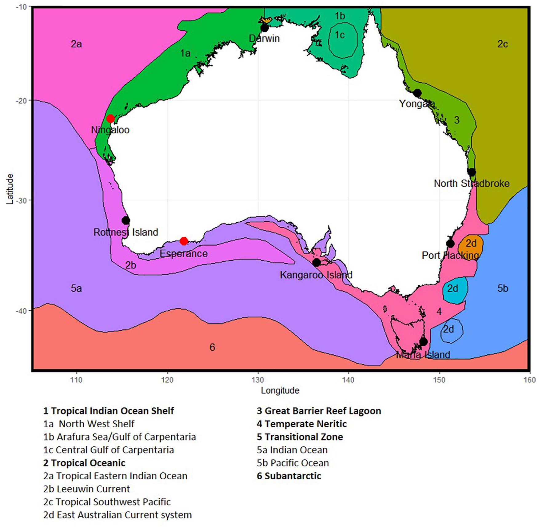
Figure 1. Location of National Reference Station sites around Australia, showing phytoplankton provinces, based on Hallegraeff et al. (2017) and Hayes et al. (2005). Note Ningaloo and Esperance (shown as red dots) are no longer sampled due to resource constraints, and Darwin and Kangaroos Island have seasonal sampling (see section 2.1).

The IMOS NRS biological dataset provides species-level information for both phytoplankton and zooplankton, as well as related physical and chemical parameters. Data on phytoplankton and zooplankton community composition is critical for assessing lower trophic level and ecosystem responses to environmental change (Edwards et al., 2010), and plankton are well established indicators for estuarine (Paerl et al., 2007), coastal (Klaiss et al., 2015) and oceanic systems (Richardson et al., 2006; Racault et al., 2014). Phytoplankton are sensitive to variations in the surrounding environment, as they have specific temperature and light regimes (Miller, 2003; Valdes-Weaver et al., 2006), and their high surface area to volume ratio enables rapid response to nutrient availability. Many phytoplankton have fast growth rates, resulting in often spectacular increases in biomass under favourable conditions (Smayda, 1990). Deviations from typical patterns of species dominance and biomass through space and time can be used to detect anomalous conditions, range expansions and potential bottom-up trophic effects (Thompson et al., 2009; McLeod et al., 2012; Hallegraeff et al., 2017). Zooplankton respond to environmental conditions such as temperature and food availability, with herbivorous plankton shaped by phytoplankton community composition, abundance, size, and nutritional value (Beaugrand, 2005; Chiba et al., 2006), as well as the timing of seasonal blooms (Edwards and Richardson, 2004). Long-term records are thus critical for detecting shifting or uncharacteristic temporal and spatial plankton cycles (Thompson et al., 2009; Johnson et al., 2011; Ajani et al., 2014).

There are a number of unique challenges in the routine collection and analysis of biological samples compared with data from sensor or laboratory measurements of physico-chemical parameters. These include issues around quantitative sampling of patchy communities whose individuals can exhibit different behaviours over space and time, and representative preservation of biological material for later analysis. As each species has a unique environmental niche, many of the questions associated with global change require that organisms are identified to the lowest possible taxonomic level, preferably to species. Microscopic analysis can be time-consuming, with a need for a high level of training of specialist taxonomists and para-taxonomists to consistently and accurately identify and quantify taxa from diverse biological communities. These unique challenges to sampling biology have contributed to the sparsity of long-term plankton records, despite their acknowledged value for ocean observation systems (Edwards et al., 2010).

Nine NRS formed the original continental-scale observation network in IMOS (Table 1). The core of the NRS network are the three historical physico-chemical coastal stations that have been sampled monthly since the 1940s and 1950s: Port Hacking (PHB, New South Wales), Maria Island (MAI, Tasmania) and Rottnest Island (ROT, Western Australia) (Lynch et al., 2014). In 2009, IMOS added six “new” NRS sites to this existing network: vis. Kangaroo Island (KAI, South Australia), Esperance, and Ningaloo (ESP, NIN, Western Australia), Darwin (DAR, Northern Territory), Yongala and North Stradbroke Island (YON, NSI, Queensland) (Figure 1 and Table 1). These “new” NRS were identified based on the principal ocean currents and associated marine environments of the Australian coastal region, the strong latitudinal gradients observed in plankton communities, the identified phytoplankton provinces, the location of National Marine Reserves and IMOS research themes, and identified priority regions (Hayes et al., 2005). Unfortunately, both Ningaloo and Esperance NRS were discontinued in 2013 because these sites are the most remote from capital cities (>1,100 and >700 km, respectively) and thus difficult to routinely service, leaving a network of seven sites. Even with the accepted value of the NRS network, maintaining long-term monitoring sites through political and science funding cycles is challenging.

TABLE 1

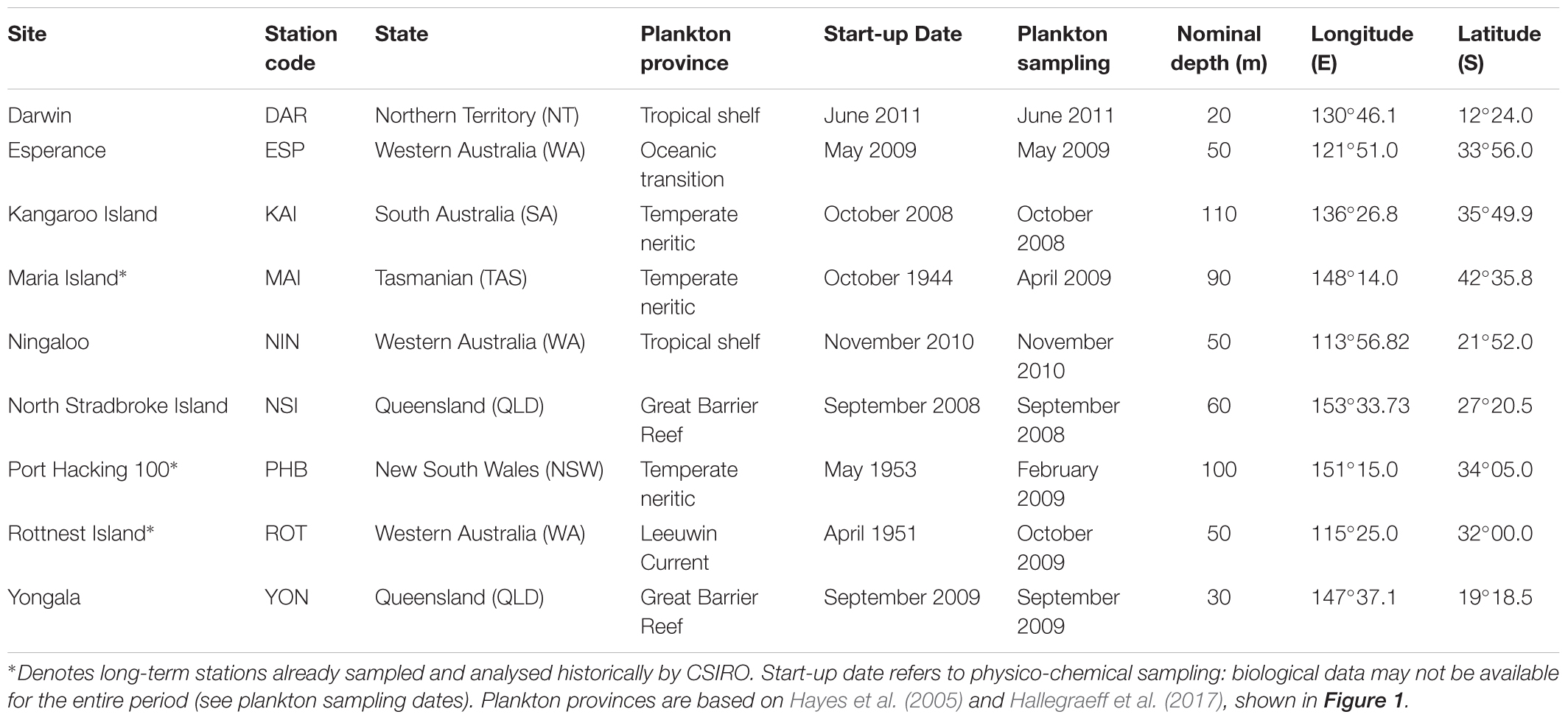
Table 1. National Reference Station codes, depths, and locations (WGS84).

2. National Reference Station Biological Sample Program

Protocols and methodologies for sampling, analysis, and data flow are documented in the IMOS NRS Biogeochemical Operations Handbook (Davies and Sommerville, 2017) and can be accessed on-line¹. NRS protocols are guided largely by standards developed for the World Ocean Circulation Experiment (Thompson et al., 2001) and Joint Global Ocean Flux Study (JGOFS, 1991) program, and in-line with Global Ocean Observing System (GOOS) principles and associated Essential Ocean Variables (Miloslavich et al., 2018a,b). Details of instrumentation, sampling equipment, calibration, preservation and transport/storage for non-biological samples are not discussed in detail here, and the reader is referred to Lynch et al. (2014).

2.1 Sampling Frequency

Phytoplankton and zooplankton are sampled monthly for composition and biomass at five of the NRS (Yongala, North Stradbroke Island, Port Hacking, Maria Island, and Rottnest Island), with seasonal sampling at Darwin and Kangaroo Island. At the Darwin NRS there are four samples taken over the tidal cycle on two of the four sampling occasions (Figure 2). There are gaps in time series at all sites due to weather conditions, and in the long-term NRS (Maria Island, Port Hacking, and Rottnest Island, Table 1) due to interruptions associated with conflicting funding priorities (Thompson et al., 2009; Ajani et al., 2014; Lara-Lopez et al., 2016). Before their termination, the Ningaloo and Esperance NRS were sampled quarterly. Field sampling is undertaken by various IMOS partners (South Australian Research and Development Institute, New South Wales Office of Environment and Heritage, Australian Institute of Marine Science and Commonwealth Scientific and Industrial Research Organisation – CSIRO) dependent on NRS location.

FIGURE 2

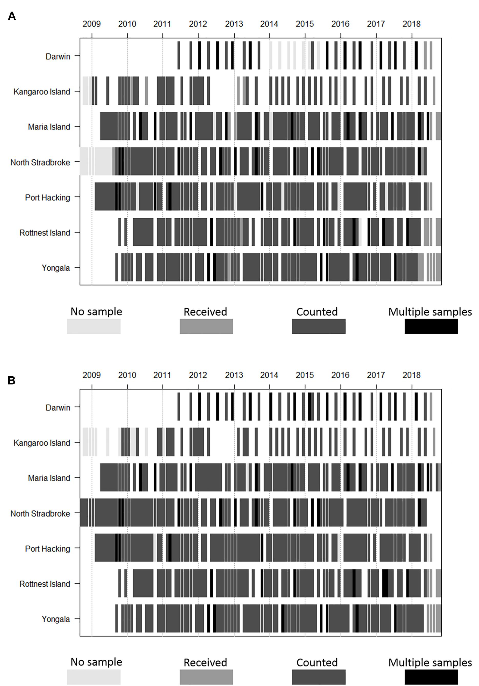
Figure 2. Frequency and duration of (A) phyto- and (B) zooplankton monitoring time-series at NRS stations, under IMOS. Note that Ningaloo and Esperance (not shown) are no longer sampled due to resource constraints and that Darwin and Kangaroo are samples are collected seasonally.

2.2 Phytoplankton Sampling and Counting

Samples for phytoplankton community composition (using light microscopy) are collected from a pooled sample prepared by collecting water from a number of discrete depth samples. Five litre Niskin bottles are fired at the surface and each 10 m depth interval (up to and including 50 m at the deeper sites) and equal volumes of water from each depth are mixed and then sub-sampled. A one litre sample is preserved in the field with Lugols iodine (acid recipe at a rate of 5 mL/L of sample), and stored in the dark until processing. A single composited sub-sample (i.e., no field replicates) is collected from the NRS due to time and budget constraints. Samples are pre-concentrated by sedimentation of the one litre composite sample, as per the method of Sournia (1978). The initial volume is reduced to 100 mL by syphoning off the supernatant after a minimum of 24 h settling time, and the sample transferred to a 100 mL cylinder and again allowed to settle for at least 24 h. The sample is further reduced to ∼10 mL, with the initial and final volumes used to calculate a concentration factor. A 1 mL sub sample is then quantitatively transferred to a Sedgewick-Rafter chamber and examined under phase contrast using a Leica DM2000 with Canon EOS 5D camera and imaging software. Count methods are based on those recommended by Hötzel and Croome (1999), with the entire chamber scanned at low magnification (×10) for large/rare taxa such as Noctiluca, Rhizosolenia, and Proboscia. The sample is re-examined at ×20 magnification until 300 cells of the dominant species have been recorded, or 400 squares (8 rows) of the chamber have been examined. Only cells >10 μm are included in this count. Instances where there are high densities of one species, a “bloom” counting rule is used, such that 300 of the dominant species is counted (and number of squares observed noted), and then the analysis is continued until 2 rows (100 squares) are counted for all other species to ensure that sample diversity of non-bloom species are recorded.

For flagellate or small species in the 5–10 μm range, a scan is conducted using a ×63 long working distance objective, until 200–300 flagellates (total count) have been recorded, or 20 squares (1 column) of the chamber has been examined. Identification of cells to species in this size class is difficult; identification is usually made to broad groups (e.g., Cryptophyte, Prasinophyte, Haptophyte), and where this is not possible, cells are grouped into simple geometric shapes (round, fusiform) for the purposes of biovolume/biomass calculations. Due to the high sediment load typically associated with Darwin phytoplankton samples (the station is within the harbour in <20 m water depth), only 1 of the 4 samples collected over the tidal cycle is processed (the one with the lowest sediment load). The sediment load at Darwin precludes an estimate of flagellates or small species around 5 μm, so count data does not include this size class.

Unknown species and good specimens of rare species may be photographed and sent to expert collaborators for identification. Results for all taxa are reported as cells/L. Estimates of biomass are calculated by assigning a geometric shape (or combination of shapes) that best describe the volume of the species/group, and volume calculated from our own or published measurements of cell size (Hillebrand et al., 1999). Biovolume data are reported as mL/L, for all taxa except tintinnids and ciliates.

2.3 Zooplankton Sampling and Counting

Zooplankton samples are collected with a Heron (1982) drop net (100 μm mesh size, 60 cm opening). Although 200 μm mesh size has been recommended as a global standard in the ICES Zooplankton Methodology Manual (Harris et al., 2000), most work is conducted in temperate and polar waters where larger zooplankton are present. As much of Australia is tropical and has smaller zooplankton present (Mckinnon et al., 2007), we have opted to use a 100 μm mesh. The Heron drop net is a vertical free-fall net with a weighted ring to propel it down at ∼1 m/s, sampling on the way down. The net is closed after a preselected time by a strangling rope secured to the boat, and then retrieved with a winch. The preselected time varies with site but it is generally within 5 m of the sonic bottom. The Heron net does not include a bridle in front of the net that larger and more active zooplankton could detect, thus avoiding capture. The depth and volume filtered by the net is unaffected by drift. A flowmeter is not attached (uncalibrated flowmeters can be the bane of biological oceanographers), as the depth accuracy is within 3.3% of the actual depth over a drop of 50 m (Heron, 1982). The volume of water sample (V_sampled) in cubic metres is calculated from Equation 1, where r = radius of the net opening.

$$V_{sampled}=(r^2)\times \pi \times dropdepth(m)\mathrm{\left(}\mathrm{1}\mathrm{\right)}$$

Three samples are taken; two are preserved in the field with 10% formalin and used for biomass (destructive analysis) and species composition (taxonomic analysis). The third sample is frozen, without formalin, and is stored at -80°C for genomics analysis, although sub-sampling for zooplankton genomics temporarily ceased in June 2017. Sampling will resume in early 2019.

Biomass is determined by filtering one formalin preserved sample through a 70 μm mesh, rinsing with freshwater, and quantitatively transferring the material to pre-weighed petri dishes. Samples are dried at 60°C for 24 h, and then re-weighed. Results are expressed as mg/m³ dry weight.

Community composition is performed on the second formalin preserved sample, using a Leica M165C dissecting scope with Canon EOS 5D camera and imaging software. Samples are concentrated for processing by passing the sample through a 70 μm sieve and re-suspending the sample to 100 mL. Depending on the quantity of plankton in the sample a 1, 2.5, or 5 mL subsample is taken using a Stempel pipette. The subsample is then washed through a 70 μm sieve (to remove the formalin) prior to counting in a Bogorov tray. A total of 50 adult copepods and 250 zooplankton are counted. If these conditions are not met, a second subsample is taken. If over 250 zooplankton have been counted in total, but less than 50 adult copepods were counted, then a second subsample is taken and only the adults are counted.

Copepods are sexed and staged, and identified to the lowest taxonomic group possible (usually species), following dissection and examination of key features. Other zooplankton groups (e.g., Chaetognaths, Appendicularians) are identified to the lowest level possible. Unknown species and good specimens of rare species may be photographed and sent to expert collaborators for identification. Selected phytoplankton species (Noctiluca, Trichodesmium) as well as tintinnids and forams are also enumerated in the zooplankton net samples. Results are expressed as abundance (individuals/m³ water filtered), according to equation 2, where V_initial is the sample volume, typically100 mL and V_counted is the sample volume analysed:

$$Individuals/m^3=(V_{initial}/V_{counted})\times (numberofindividuals/V_{sampled})\mathrm{\left(}\mathrm{2}\mathrm{\right)}$$

2.4 Zooplankton Size Spectra

Body size has been described as the “master trait,” setting the pace of life by dictating processes such as metabolism, respiration, development, movement, and is the basis for many food web models (Blanchard et al., 2017). In addition to microscopic examination of the formalin-preserved sample, we use two complementary methods to measure the zooplankton size spectrum, each with strengths and weaknesses. The Laser Optical Plankton Counter (LOPC) is a rapid assessment method utilising a series of lasers to measure the size and number of particles (see Herman et al. (2004) for more details). There is no taxonomic information provided and it is difficult to discriminate detritus and sand. A more detailed method for obtaining size information is the ZooScan system² a laboratory flatbed scanning system that digitises preserved zooplankton samples (Gorsky et al., 2010). The high quality images are processed using the artificial neural network imaging software, ZooProcess (Vandromme et al., 2012). Using the ZooScan/ZooProcess system has the benefit of classifying specimens into functional groups (e.g., calanoid copepods, chaetognaths, siphonophores) and removing detritus from the analysis, but comes with much longer processing time. We see these and other more automated techniques as highly complementary to the more labor-intensive species level taxonomic discrimination afforded by microscopy, and they provide useful tools for parallel studies at the local or regional scale where species level taxonomy may not be possible, or desirable.

2.5 Auxiliary Information

Auxiliary information useful for interpretation of plankton data from NRS sites is available through instrumentation associated with the in situ moorings and field-based measurements and samples collected during monthly sampling events. Related measurements include standard oceanographic parameters such as salinity, temperature, dissolved oxygen, pH, PAR, fluorescence and turbidity, and samples collected for calibration and performance monitoring of biosensors, pigment analysis by HPLC, and analysis of picoplankton by flow cytometry (Table 2). Recently, sampling efforts have been expanded to include ichthyoplankton (Smith et al., 2018) and microbial communities (Brown et al., 2018). Data from all related measurements in Table 2 are available from the Australian Ocean Data Network (AODN) portal³. All dates and times associated with sample data are in UTC, as there are different time zones in Australia and daylight saving in summer is also not uniform around the country.

TABLE 2

Table 2. Parameters measured in situ, or sampled at National Reference Station sites, with instrument type or method, and units.

3. Data Management And Usage

As at October 2018, data from a total of 678 zooplankton and 580 phytoplankton NRS samples have been acquired, (with over 100 samples collected at each of the monthly stations of NSI, MAI, PHB, ROT, YON; see Table 1 for site codes) spanning 10 years of IMOS sampling. All data is available through the AODN as either a raw data product, or binned data products (functional groups, genus, species) that are “analysis-ready,” and take absences and taxonomic changes into account (see sections 3.2 and 3.3).

Summaries of the total number of taxon observed, the average number of taxa per sample, and the total number of samples counted at each NRS are shown in Figure 3 (phytoplankton) and Figure 4 (zooplankton), with a summary of the major taxonomic groups observed at each NRS presented in Figures 5, 6. Phytoplankton community composition (presented as biovolume due to the high abundance of flagellates masking diversity of other groups) varies with the phytoplankton provinces described by Hallegraeff et al. (2017). The cooler waters of the Temperate Neritic province (PHB, MAI, KAI) are noted for the seasonal succession of small diatoms to large dinoflagellates over spring and summer, and the presence of Noctiluca. The Great Barrier Reef Lagoon province (YON, NSI) are remarkably similar, with more than 90% of the biovolume associated with centric diatoms. NRS stations on the Tropical Shelf (DAR, NIN), Leeuwin Current and Tropical Oceanic (ROT, ESP) are similarly dominated by centric diatoms, however, the high sediment load in Darwin Harbour limits discrimination by light microscopy, and masks the true species diversity of the region. Pigment analysis by HPLC can provide important information on the community composition at this site.

FIGURE 3

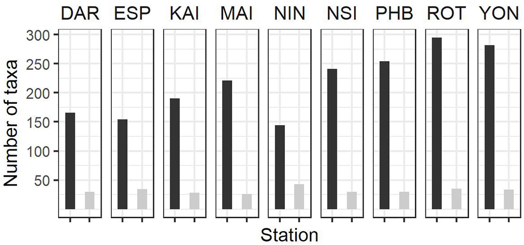
Figure 3. Summary of phytoplankton count data at the NRS (dark bars, total number of taxa per station; light bars, average number of taxa per sample) since IMOS commenced network observations. See Table 1 for start date of IMOS plankton time series at each location. DAR, Darwin (n = 31); ESP, Esperance (n = 17); KAI, Kangaroo Island (n = 47); MAI, Maria Island (n = 96); NIN, Ningaloo (n = 12); NSI, North Stradbroke Island (n = 100); PHB, Port Hacking (n = 100); ROT, Rottnest Island (n = 87); YON, Yongala (n = 96) where n = number of samples counted at each station.

FIGURE 4

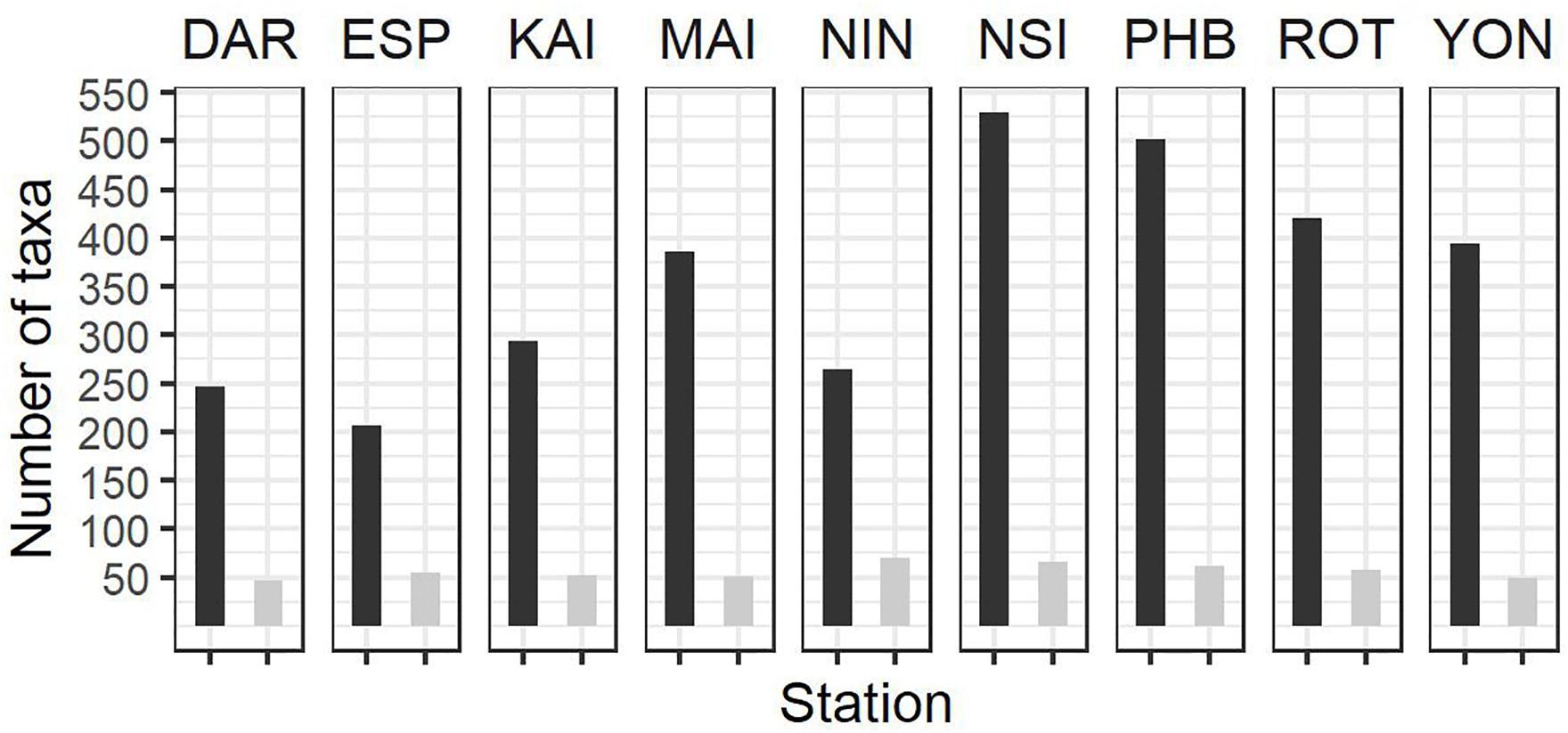
Figure 4. Summary of zooplankton count data at the NRS (dark bars, total number of taxa per station; light bars average number of taxa per sample) since IMOS commenced network observations. See Table 1 for start date of IMOS plankton time series at each location. DAR, Darwin (n = 31); ESP, Esperance (n = 17); KAI, Kangaroo Island (n = 41); MAI, Maria Island (n = 100); NIN, Ningaloo (n = 12); NSI, North Stradbroke Island (n = 114); PHB, Port Hacking (n = 179); ROT, Rottnest Island (n = 91); YON, Yongala (n = 98 where n = number of samples counted at each station.

FIGURE 5

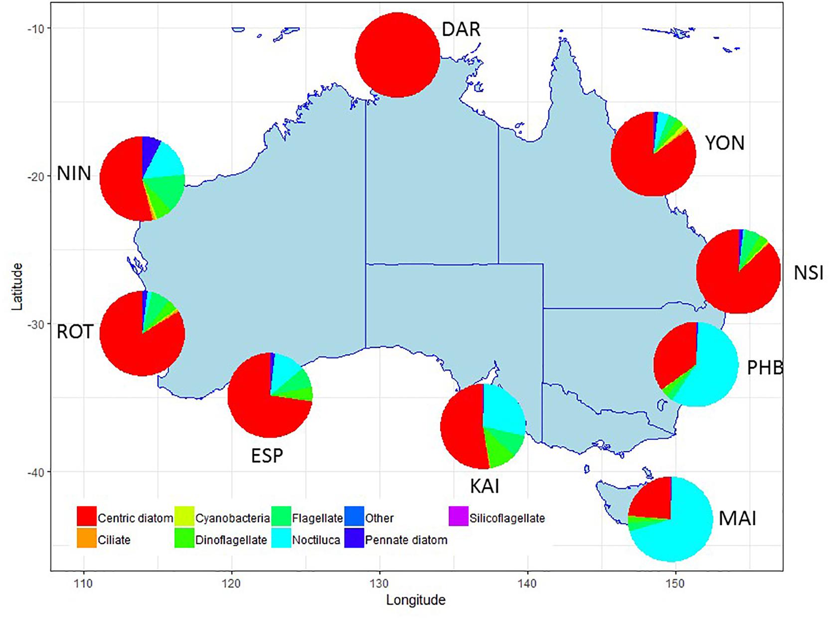
Figure 5. Major taxonomic or functional groups of phytoplankton taxa counted in the NRS survey, all samples combined. Phytoplankton data presented as biovolume (μm³/L) due to the high proportion of flagellates in abundance data. Site details and codes are as per Table 1.

FIGURE 6

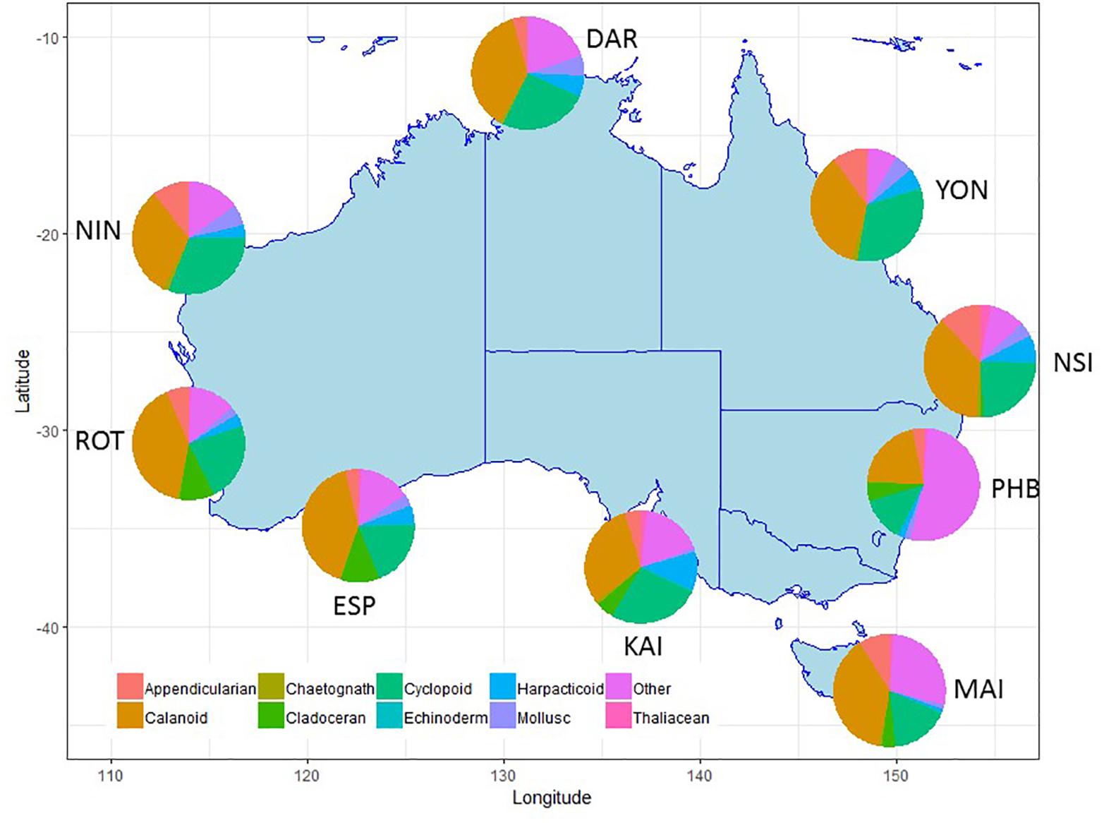
Figure 6. Major taxonomic or functional groups zooplankton taxa counted in the NRS survey, all samples combined. Site details and codes are as per Table 1.

Within the zooplankton, copepods (calanoid, harpacticoid and cyclopoid) consistently dominate abundance data making up 45–70% across all stations, however, there are clear differences in the copepod species contributing to tropical, sub-tropical and temperate communities (Lynch et al., 2014).

3.1 Data Entry

Immediately on completion of counting a sample, data are entered into an Oracle database, which forms an integral part of laboratory and data quality control (see later discussion on taxonomic changes and QA/QC in sections 3.3 and 4.4). Data entries are double-checked to prevent errors. Count data (phytoplankton abundance, cells/L and biovolumes, μm³; zooplankton abundance, ind/m³ and biomass, mg/m³) for each NRS are automatically transferred from the CSIRO Oracle database to the Australian Ocean Data Network (AODN) portal every evening at midnight, where it is then available on-line³. Conversion of phytoplankton biovolume data to carbon biomass (pg C/cell) may be undertaken using the equations in Davies et al. (2016).

3.2 Abundance and Presence/Absence Records

All taxa encountered are entered as count data – i.e., there are no categories for recording presence only during sample analysis. Counts data can be converted to presence/absence data if required. Absences require special consideration, and these are taken into account in the binned products available on the AODN. Absences can be inferred from the raw data for any of the taxa that we have counted over the life of the project, but are not present in a particular sample count. For more information on dealing with absences for time-series analysis, refer to section 3.3.

3.3 Taxonomic Notes and Validity of Names

Appropriate use of the NRS data requires a clear understanding of the sampling and analysis methods, and the level of taxonomic discrimination routinely possible using light microscopy techniques. A comprehensive list of taxa recorded at each of the NRS is presented in Supplementary Table 1 (Phytoplankton) and Supplementary Table 2 (Zooplankton, copepods) and Supplementary Table 3 (Zooplankton, non-copepods). These tables include taxonomic notes relating to the use of taxon, and groupings where uncertain identification can lead to clumping or use of “bucket” categories. Zooplankton taxa recorded include 561 copepod taxa (237 species), and 290 non-copepod taxa (72 species) with 99 species occurring in more than 1% of samples. A total of 541 phytoplankton taxa (286 species) have been recorded, and of those, 222 occur in more than 1% of samples.

It is not uncommon for taxonomic names to change following revision by experts, especially with the well-established use of genetic techniques to clarify taxonomy and relationships between species and genera. Accepted name changes are typically tracked through the scientific literature, and communications with expert collaborators. Each species name recorded in the NRS phytoplankton and zooplankton datasets are consistent with the current accepted scientific name according to WoRMS (World Register of Marine Species⁴). When a new name for an existing species is verified in WoRMS, all records in the plankton database are updated to reflect contemporary taxonomy. For example, the dinoflagellate genus Ceratium has been through significant review in recent years, and is now Tripos. All records previously entered while Ceratium was a valid taxon name will now appear as Tripos, for the entire period of samples counted.

For taxa where identification to species cannot be achieved (either because the specimen is in poor condition, or incomplete), a higher taxonomic level has been applied. In instances where reliably distinguishing between species is not possible because of the limitations of light microscopy, size-based taxon groups have been created, i.e., Thalassiosira spp. 10–20 μm, Pseudo-nitzschia delicatissima group <3 μm diameter.

As the NRS program matures, there are improvements in the taxonomic resolution recorded over time by our analysts. This issue is particularly important for those using the data for time series analysis, or interpreting species absences. A taxonomic change log (maintained in the Oracle database) is attached to each record downloaded from the AODN, which documents the name that the taxa has been previously assigned, the date of training, and the name it will be assigned in the future. For example, before September 2012 we identified Oncaea media only as a species complex. All entries before this date do not discriminate between the species within the complex, and are identified as Oncaea media complex. After training on this date we were able to identify the species within the complex and we now use Oncaea media, O. waldamari, and O. scottodicarlo and retain O. media complex when further discrimination is not possible. Each of these species would have been present in the original category of O. media complex so their absence from the data prior to the training date should not be considered a true absence. This is particularly critical information when analysing time series.

3.4 Data Availability

In addition to specific data queries for NRS data that can be generated through the AODN, there are several significant compilations of historical data from the Australian region that help put the IMOS plankton data into a longer-term and broad-scale context. These include historic phytoplankton species data (the Australian Phytoplankton Database; Davies et al., 2016), historic chlorophyll a data (the Australian Chlorophyll Database; (Davies et al., 2018), historic zooplankton species data (the Australian Zooplankton Database; (Davies et al., 2014), and historic zooplankton biomass data (the Australian Zooplankton Biomass Database; currently under development with records from the NRS⁵ and Continuous Plankton Recorder⁶ available via the AODN). These compilations and all associated ancillary IMOS data from the NRS are publicly available from the AODN with a Creative Commons BY licence, with acknowledgement of the data source a requirement. Typically, data usage should be acknowledged through statements such as “Data were sourced from the Integrated Marine Observing System (IMOS). IMOS is a national collaborative research infrastructure, supported by the Australian Government.”

For plankton data there may be a delay of some months between sample collection and data upload, with a target of all data publicly accessible within 6 months. Once a sample is collected, it is often retained for several months so that multiple samples can be sent together to the CSIRO laboratories for analysis to save money.

4. QA/QC Measures

4.1 Identification

Primary taxonomic references used for phytoplankton species identification include Tomas (1997); Scott and Marchant (2005), and Hallegraeff et al. (2010), and literature cited therein. Other more-site-specific taxonomic resources are used where available, for example Port Hacking publications by Wood (1964), Hallegraeff (1981), and Ajani (2014). Primary references for zooplankton identification include Dakin and Colefax (1940), Bradford-Grieve (1994, 1999), Boltovskoy (1999a,b), Conway et al. (2003), Razouls et al. (2005–2019)⁷ and numerous other resources listed on the Australian Marine Zooplankton website⁸ (Swadling et al., 2013). Some larger taxon may be identified and counted in both zooplankton and phytoplankton count procedures (for example Noctiluca, Trichodesmium, tintinnids and forams).

4.2 Analyst Training

Consistency of taxonomic data is critical for long-term biological datasets where trends are used to interpret habitat condition, biodiversity and changes over time. To maintain a high and consistent level of taxonomic classification, analysts involved in identification and data generation for NRS samples instigate, design and attend annual training workshops for both phyto- and zooplankton. Workshops are typically 3–5 days in duration and include instruction from, and discussions with expert collaborators who are familiar with species-level identification. Workshops include examination of archived samples, mono-cultures, and live samples, with a focus on inter-analyst variability, identification of unknowns, and the development of identification guides and species reference sheets (see section 4.3). Classification of groups of phytoplankton species that are difficult to discriminate by light microscopy are reviewed annually at training workshops, in light of contemporary information and techniques in the scientific literature.

4.3 Reference Collections and Species Reference Sheets

Digital reference collections are maintained for all NRS phytoplankton and zooplankton species through an image database (currently only available internally); there is also a physical collection of zooplankton specimens. Unknown phytoplankton and zooplankton specimens and tentative identifications are digitally photographed and routinely distributed to expert collaborators for confirmation and identification.

An important part of ensuring consistency between multiple analysts is the internal development and use of species reference sheets. These are compilations of published information and diagrams, useful diagnostic aids, and images and size measurements sourced from samples collected in Australian waters and prepared in a standard format. The Australian Zooplankton Atlas⁹ (Swadling et al., 2013) contains reference sheets and other useful information, produced in collaboration with zooplankton experts. Phytoplankton reference sheets are developed on an on-going basis, and are reviewed by taxonomic experts and will be collated in the Australian Phytoplankton Atlas for broader use among the marine plankton community. Over time, the information compiled in the species reference sheets is transferred to interactive taxonomic keys using the Lucid software¹⁰.

4.4 Counting and Identification Protocols

The database was developed specifically to manage biological data, and is a central tool to ensure data quality and consistency. It is not possible to enter data more than once for each sample (i.e., no double entry of data), and data must be cross-checked back to the original datasheet before the database can be updated. Warnings are generated for the use of invalid taxa, or abundances that lie outside of 2 standard deviations from the mean for that taxon. Currently accepted nomenclature is regularly checked using the WoRMS website, with the database updated with any changes so that nomenclature, spelling and taxonomic groupings are consistent.

The date that each taxon commenced being used (and finished for invalid taxa) is recorded internally in the database, as well as the identity of the person who enters the data, allowing us to track biases, and/or increases in resolution of particular genera. Each taxon is mapped to the NRS location where it has previously been identified, thus flagging each time a taxon is recorded at a new location. Images of unknowns documented during analysis can be linked to each sample entry, along with the verified name and expert associated with the identification.

Clear counting rules have been developed for all major taxonomic groups observed to prevent double counting. For zooplankton, these rules include counting only heads of Chaetognaths and tails of Appendicularians, and only prosomes or urosomes of damaged copepod specimens. For phytoplankton, these rules include only counting cells with chloroplasts or cell contents intact, and for long or fragile genera like Rhizosolenia and Proboscia, only counting cell fragments with a valve intact. Colonial or chain forming species are counted if they overlap the upper or left boundary of the Sedgewick Rafter counting square, but not if they overlap the bottom or right boundary of the counting square. Over time, the amount of effort counting a sample has been reviewed by analysing counting statistics to bench mark whether a reduction in counting effort (proportion of sample or counting chamber analysed) will still accurately represent both abundance and diversity. These analyses contribute to updates to counting rules specifying the minimum total number of individuals that should be counted (see section 5.5).

5. Lessons Learnt

5.1 Partnering With Physical and Chemical Oceanographers for Sustained Funding

The foundation of any long-term observation system is sustained funding. IMOS has successfully attracted an annual investment of around $A18M for the past 10 years because the Australian marine research community united around the common goal of marine observation in the context of a changing world. IMOS is a broad program covering physical, chemical and biological observing systems, with sufficient flexibility that as government priorities change, there are many parts of the observing system that can deliver relevant responses (Lara-Lopez et al., 2016). Diverse data streams produced by IMOS have been integral in responding to many pressing government and industry priorities, including: better managing eutrophication on the Great Barrier Reef to help maintain its World Heritage status (Brodie et al., 2017); mitigating risks associated with carbon sequestration under the seafloor¹¹; providing integrated baselines and assessments to support the oil and gas industry (Kloser and van Ruth, 2017); identifying the best search locations to find the Malaysian Airlines flight MH370 (Maclaughlin, 2017); providing advice for locating ocean turbines to generate the most renewable energy and describing the movements of recreational and commercial fish species to inform fisheries management (Brodie et al., 2018). The plankton observing system is only a small part of the whole system and would be unlikely to attract sustained funding in isolation. Partnering with the broader observing system community has been key to exerting political influence and developing a world class biological observatory.

5.2 Human Capital

If funding is the foundation of an observing system, human capital (or expertise) is the structure. It is challenging to maintain and develop consistent expertise over the duration of long-term observation program. Whilst consistency in biological observations is tied to retention of appropriately skilled analysts, we have found that to meet our milestones we need multiple team members who have expertise in each of phytoplankton identification, zooplankton identification, hierarchical databases, statistical analysis, photography and working with social media. This built in redundancy has led to more resilience in our delivery of regular milestones in the event of staffing changes, and has helped to inoculate against boredom. The need to constantly improve our taxonomic knowledge has been a particular (but welcome) challenge for a continental-scale observing system reliant on expertise in tropical, sub-tropical, temperate and sub-Antarctic plankton communities.

5.3 Partnering With Taxonomic Experts

Opportunities to formally train in plankton taxonomy in Australia are rare, and diminishing. We have developed much of our taxonomic expertise by partnering with senior practising taxonomists around the world. The willingness of taxonomists to give of their time to help with initial and ongoing training is humbling, and has resulted in an increase in the known plankton diversity in Australia through the NRS samples. For example, as in most zooplankton surveys, we originally identified the cyclopoid Oncaea only to genus level. Following a visit by Dr. Ruth Bottgner-Schnack, an international specialist in Oncaea, we now identify 11 species, including several not previously identified from Australian waters. Being able to capture digital images and sending these to our network of collaborators has meant that we are not only able to verify unknown specimens, but also improve their taxonomic resolution in our region. Our taxonomic collaborators have also given of their time in annual taxonomic workshops. The capacity to identify taxa to species is especially important for resolving biological diversity around Australia’s, see for example phytoplankton provinces (Figure 1). We have recently completed a major revision of the dinoflagellate genus Tripos in Australian waters using data from the NRS, under the guidance of Professor Gustaaf Hallegraeff who has provided training in this genus since the program inception.

5.4 Importance of a Relational Database

We believe it is impossible to run a continental-scale biological observing program without a relational database. The database streamlines data entry through templates and forms, improves quality control, and enables automatic and routine export of data to online webservers. We are able to write queries to manipulate and extract the data for specific analyses, and to maintain taxonomic consistency through updates to taxonomic nomenclature tables and associated lists of authorities, and manage data queries that consider the changing taxonomic capabilities through the change log (see section 3.3). The database has also been instrumental in developing and maintaining significant compilations of IMOS and collaborators plankton data from the Australian region for phytoplankton, zooplankton, biomass and chlorophyll a collections (see section 3.4).

5.5 Streamlining Methods

Consistency in time series is key to maintaining robust data streams. Funding cutbacks in the first decade of the observatory triggered a necessary reassessment of laboratory processing protocols. Counting of samples to species level is time intensive, but necessary if we wish meet our objective to use plankton data to monitor change. Using the database to keep track of how long samples take to count, and the associated diversity at each of the NRS, we analysed whether a reduction in counting effort could be made without losing information on abundance and diversity. For example, up until the end of 2015, the mean time it took to count an NRS zooplankton sample was 5.1 h, and nearly 5% of the samples took >10 h. Initially we took a subsample (1, 2, or 5 mL) and counted at least 500 individual zooplankton and 100 adult copepods. If we did not reach that number after counting the subsample, then we took another sub-sample and counted it completely. As part of revising protocols in 2015, we conducted a simulation study to assess what would happen if we changed this counting procedure. We found that if we count 250 individual zooplankton and 50 adult copepods, then there would be minimal impact on abundance estimates and community analyses (Figure 7). Implementing this change in counting has reduced mean counting time from 5.1 h to 3.1 h. We also found that if we changed to counting a set volume to reduce time, there would be very different data produced in terms of diversity, as more rare taxa would be lost. If we had not changed our counting procedures so we could count the same number of samples with less money there was a strong possibility of our funding being discontinued. However, we ensured that changes were carefully thought through so they had minimal impact on consistency. Similar analyses were conducted for the phytoplankton counts and amended count procedures implemented in June 2016.

FIGURE 7

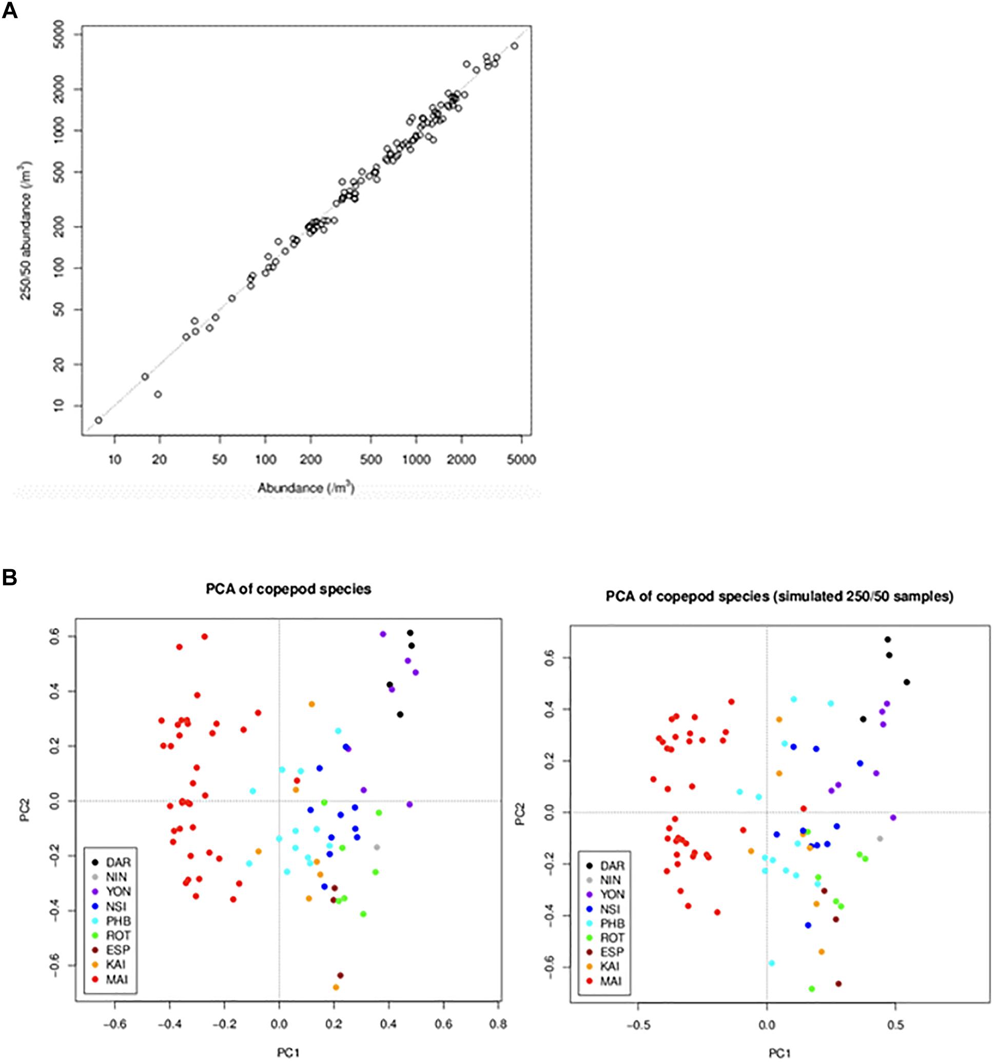
Figure 7. Comparison of data obtained under the initial and revised counting rules. Data obtained under the new rules (250 individuals/50 adults) were simulated from data obtained under the old rules (500/100). To simulate the new-rule data for a sample, we selected a subset of the sample’s subsamples that was consistent with the new rules. The graphs compare data from the old and new rules in terms of (A) copepod abundance (the dotted line is the 1:1 line) and (B) copepod community composition (summarised by principal components analysis of copepod species) (DAR = Darwin, ESP = Esperance, KAI = Kangaroo Island, MAI = Maria Island, NIN = Ningaloo, NSI = North Stradbroke Island, PHB = Port Hacking, ROT = Rottnest Island, YON = Yongala).

5.6 Product Development to Extend Uptake and Improve Impact

Research impact through publications is often not the only metric by which long-term observing program are judged. Increasingly, government funders expect observing systems to have measurable impacts supporting marine management. There are two main areas of product development where we have been able to expand our impact. The first is in ecosystem assessments, which say something about the state and trends of our marine systems, from local through national to global scales. For example, the key ecosystem assessment in Australia is the Australian State of Environment Report¹². This report had case studies based on IMOS data, describing changes in harmful algal blooms, jellyfish and calcifying zooplankton. Data will be provided for upcoming assessments, such as the Great Barrier Reef Outlook Report¹³, detailing trends in the abundance of the cyanobacterium Trichodesmium, which produces nearly half of the primary production in nutrient-poor regions (Capone et al., 1997). Long-term data allows testing the hypothesis that as oceans become more stratified with global warming, Trichodesmium will increase in abundance (Beardall and Stojkovic, 2006).

The second main area of product development has been in model assessment, or validation. Biogeochemical and ecosystem models have plankton functional groups, including small and large zooplankton, diatoms, dinoflagellates, harmful algal blooms, and jellyfish, and require data for their assessment. Given the critical role zooplankton plays in the marine environment, models need to adequately capture plankton dynamics (Everett et al., 2017). Based on an examination of 153 published biogeochemical models, Arhonditsis and Brett (2004) found that <20% of them compared model output with zooplankton data. In the relatively rare instances where zooplankton were assessed in biogeochemical models, they were more poorly simulated than almost any other state variable. Gridded products are commonly used in model assessment, from SST to chlorophyll a; we have developed the first gridded products for zooplankton biomass such as that used for assessment of the eReefs biogeochemical model on the Great Barrier Reef (Skerratt et al., 2019) (Figure 8). Given that many significant management issues are tackled by biogeochemical and ecosystem models – including impacts of sediment dumping from dredging, potential management strategies for managing crown-of-thorns, assessing trade-offs of multiple-use of common fisheries resources and coastal aquaculture, and socio-economic impacts of different management decisions – products for model assessment based on plankton data can directly improve our marine management. The modelling approach also allows us to integrate other long-term plankton datasets within the IMOS Plankton Survey such as the Continuous Plankton Recorder (CPR). There are fundamental differences however in the sampling strategies (Niskins, nets and silks), frequency of sampling, and spatial scales (point or underway) of these programs. We have developed statistical approaches to combine these and other plankton observations using generalised linear models. Additional areas of data uptake include validation of “new” technologies such as automated imaging, remote sensing, acoustics and ‘omics approaches to plankton biodiversity and ecology. We believe the use of long term, quantitative microscopy-based species level datasets such as the NRS is critical to a robust assessment and cross-validation of the strengths of each of these approaches. The potential for high-frequency, broad-scale observations of the ocean using a combination of these techniques is exciting.

FIGURE 8

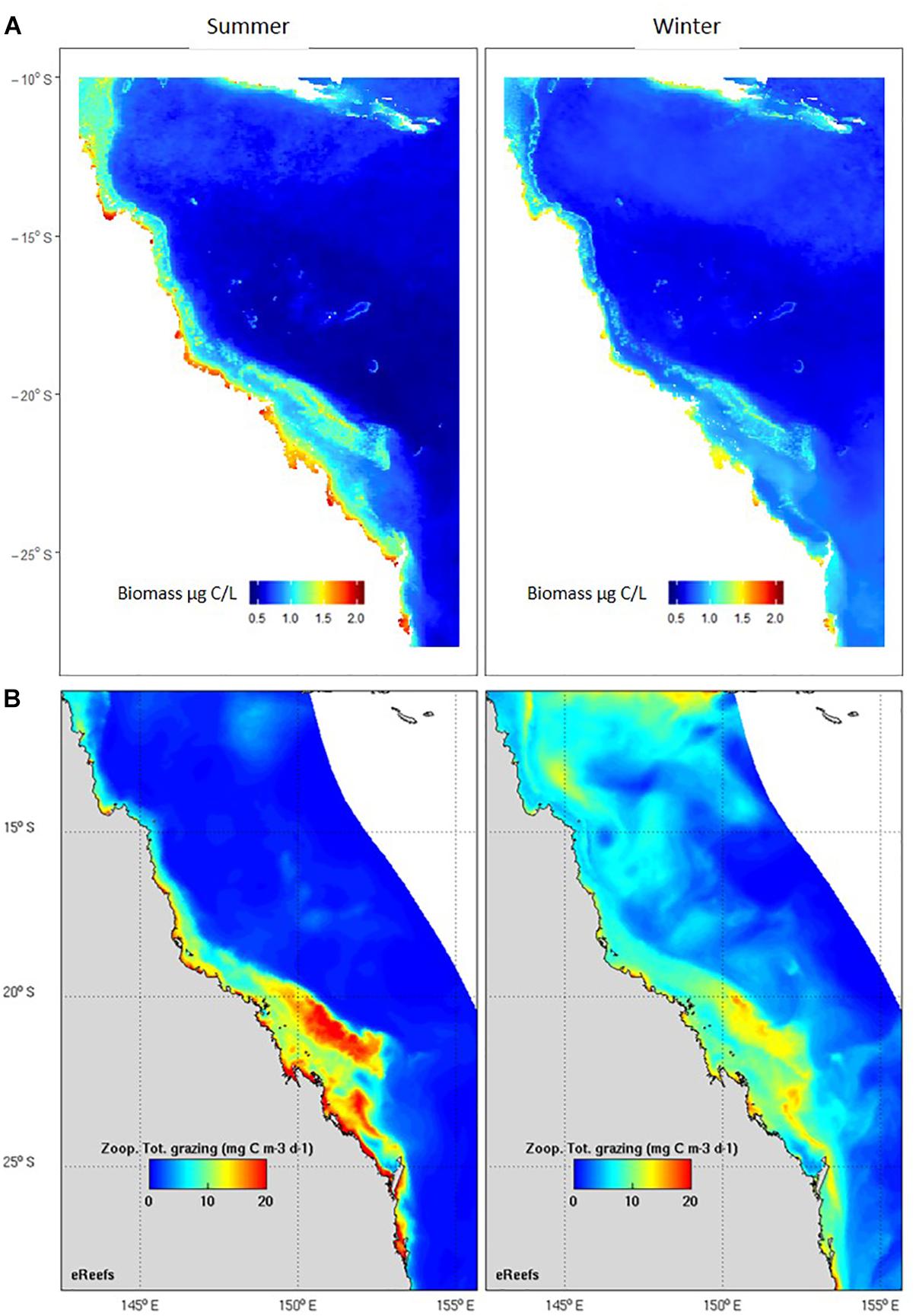
Figure 8. Comparison of seasonal observed and modelled zooplankton. (A) Zooplankton biomass (μg C/L) based on > 900 observations, including the IMOS Australian Continuous Plankton Recorder, the IMOS NRS and other zooplankton samples collected within the eReefs domain. Results are from a linear model using data from a statistical model based on mesh size, chlorophyll a, SST, depth and day of year r² = 57% (Skerratt et al., 2019). (B) Zooplankton total grazing (mg C/m3/day) output from the eReefs model (Skerratt et al., 2019).

5.7 Community Engagement

Community interest and engagement with our data is an important metric of success in communicating information about marine biodiversity to a broader audience. We have used social media platforms such as Facebook¹⁴ to highlight importance of long-term biological datasets. Posting striking images of plankton, quizzes on “what plankton is that?”, and images of our fieldwork has been well received by specialist and non-specialist followers. Recent engagement in professional development for teachers through the Educator on Board program for RV Investigator has resulted in teachers working alongside researchers to learn about plankton sampling techniques, identification and ecology. These experiences have then been incorporated into the STEM curriculum for primary and secondary students¹⁵. Other outreach activities include collaborations with The Moreton Bay Environmental Education Centre to provide opportunities for secondary school students to learn about marine ecosystems, sample and data collection methodologies and applications for research. This work included production of a short TV programme¹⁶.

Collaborations with professional photographers and artists to uncover the hidden world of plankton have been particularly rewarding.

Author Contributions

AR, RE, and CD conceived and designed the manuscript. CD, MM, and SE developed and organised the database. WR performed the statistical analysis. RE, CD, FC, JU-P, MT, AS, and FM compiled the Supplementary Material. All authors contributed to manuscript revision, read and approved the submitted version.

Funding

The National Reference Stations are part of the Integrated Marine Observing System (IMOS) – IMOS is a National Collaborative Research Infrastructure, supported by the Australian Government.

Conflict of Interest Statement

The authors declare that the research was conducted in the absence of any commercial or financial relationships that could be construed as a potential conflict of interest.

The reviewer PM declared a shared affiliation, with no collaboration, with one of the authors, RE, to the handling Editor at the time of review.

Acknowledgments

We are particularly grateful to the many taxonomic experts who we collaborate with: Dr. Penny Ajani (phytoplankton, University of Technology Sydney), Dr. Ruth Bottgner-Schnack (oncaeid copepods, Germany), Professor Geoff Boxshall (copepods, Natural History Museum, United Kingdom), Dr. Janet Bradford-Grieve (copepods, National Institute of Water and Atmospheric Research), Dr. Steve Brett (phytoplankton, Microalgal Services, Australia), Dr. Dave Conway (zooplankton, Marine Biological Society of the United Kingdom), Dr. Mark Gibbons (non-copepod zooplankton, University of the Western Cape, South Africa), Professor Gustaaf Hallegraeff (phytoplankton, University of Tasmania), Mr. Ian Jameson (phytoplankton, CSIRO), Dr. Dave McKinnon (copepods, Australian Institute of Marine Science), Dr. Antonina dos Santos (decapods, Instituto Português do Mar e da Atmosfera, Portugal), and Dr. Kerrie Swadling (zooplankton, University of Tasmania), who generously provided support in the development and on-going validation of our methods and analyses. We are also grateful for the special interest and talented work of collaborating artists Diane Masters and Julia Bennett. We would like to acknowledge the support of IMOS, in particular the Director Mr. Tim Moltmann, for his support of and belief in the plankton work and Dr. Ana Lara-Lopez. We also thank the staff at the Australian Ocean Data Network, especially Dr. Natalia Atkins. Finally, our work would not have been possible without the significant efforts of sampling crews and all providing logistical support at each of the NRS.

Supplementary Material

The Supplementary Material for this article can be found online at: https://www.frontiersin.org/articles/10.3389/fmars.2019.00161/full#supplementary-material

Footnotes

1. ^ http://content.aodn.org.au/Documents/IMOS/Facilities/national_mooring/IMOS_NRS_BGCManual_LATEST.pdf
2. ^www.zooscan.com
3. ^ https://portal.aodn.org.au/
4. ^ http://www.marinespecies.org
5. ^ https://portal.aodn.org.au/search?uuid=c13451a9-7cfc-091c-e044-00144f7bc0f4
6. ^ https://portal.aodn.org.au/search?uuid=c1344979-f702-0916-e044-00144f7bc0f4
7. ^ http://copepodes.obs-banyuls.fr/en
8. ^ http://www.imas.utas.edu.au/zooplankton/references
9. ^ http://www.imas.utas.edu.au/zooplankton
10. ^ http://www.lucidcentral.com/en-au/home.aspx
11. ^ https://www.csiro.au/en/Research/OandA/Areas/Coastal-management/Offshore-CCS-monitoring
12. ^ https://soe.environment.gov.au/
13. ^ http://www.gbrmpa.gov.au/our-work/reef-strategies/great-barrier-reef-outlook-report
14. ^https://www.facebook.com/imosaustralianplanktonsurvey
15. ^https://research.csiro.au/educator-on-board/
16. ^https://www.youtube.com/watch?v=HDVQCxsksag

References

Ajani, P. (2014). Phytoplankton Diversity in the Coastal Waters of New South Wales. Ph.D. thesis, Macquarie University, Sydney, NSW.

Google Scholar

Ajani, P. A., Allen, A. P., Ingleton, T., and Armand, L. (2014). A decadal decline in relative abundance and a shift in microphytoplankton composition at a long-term coastal station off southeast Australia. Limnol. Oceanogr. 59, 519–531. doi: 10.4319/lo.2014.59.2.0519

CrossRef Full Text | Google Scholar

Arhonditsis, G. B., and Brett, M. T. (2004). Evaluation of the current state of mechanistic aquatic biogeochemical modeling. Mar. Ecol. Prog. Ser. 271, 13–26. doi: 10.3354/meps271013

PubMed Abstract | CrossRef Full Text | Google Scholar

Beardall, J., and Stojkovic, S. (2006). Microalgae under global environmental change: implications for growth and productivity, populations and trophic flow. ScienceAsia 32, 1–10. doi: 10.2306/scienceasia1513-1874.2006.32(s1).001

CrossRef Full Text | Google Scholar

Beaugrand, G. (2005). Monitoring pelagic ecosystems using plankton indicators. ICES J. Mar. Sci. 62, 333–338. doi: 10.1016/j.icesjms.2005.01.002

CrossRef Full Text | Google Scholar

Blanchard, J. L., Heneghan, R. F., Everett, J. D., Trebilco, R., and Richardson, A. J. (2017). From bacteria to whales: using functional size spectra to model marine ecosystems. Trends Ecol. Evol. 32, 174–186. doi: 10.1016/j.tree.2016.12.003

PubMed Abstract | CrossRef Full Text | Google Scholar

Boltovskoy, D. (1999a). South Atlantic Zooplankton, Vol. 1. Kerkwerve: Backhuys.

Google Scholar

Boltovskoy, D. (1999b). South Atlantic Zooplankton, Vol. 2. Kerkwerve: Backhuys.

Google Scholar

Bradford-Grieve, J. M. (1994). The Marine Fauna of New Zealand: Pelagic Copepoda: Megacalanidae, Calanidae, Paracalanidae, Mecynoceridae, Eucalanidae, Spinocalanidae, Clausocalanidae. Wellington: National Institute of Water and Atmospheric Research.

Google Scholar

Bradford-Grieve, J. M. (1999). The Marine Fauna of New Zealand: Pelagic Copepoda: Arietellidae, Augaptilidae, Heterorhabdidae, Lucicutiidae, Metridinidae, Phyllopodidae, Centropagiidae, Pseudodiaptomidae, Temoridae, Candaciidae, Pontellidae, Sulcanidae, Acartiidae, Tortanidae, vol. 111, Auckland: NIWA Biodiversity Memoirs, 268.

Google Scholar

Brodie, J., Baird, M., Waterhouse, J., Mongin, M., Skerratt, J., Robillot, C., et al. (2017). Development of Basin-Specific Ecologically Relevant Water Quality Targets for the Great Barrier Reef. TropWATER Report No. 17/38. Brisbane, QLD: James Cook University.

Google Scholar

Brodie, S., Lédée, E. J. I., Heupel, M. R., Babcock, R. C., Campbell, H. A., Gledhill, D. C., et al. (2018). Continental-scale animal tracking reveals functional movement classes across marine taxa. Sci. Rep. 8:3717. doi: 10.1038/s41598-018-21988-5

PubMed Abstract | CrossRef Full Text | Google Scholar

Brown, M. V., Van De Kamp, J., Ostrowski, M., Seymour, J. R., Ingleton, T., Messer, L. F., et al. (2018). Systematic, continental scale temporal monitoring of marine pelagic microbiota by the Australian marine microbial biodiversity initiative. Sci. Data 5:180130. doi: 10.1038/sdata.2018.130

PubMed Abstract | CrossRef Full Text | Google Scholar

Capone, D. G., Zehr, J. P., Paerl, H. W., Bergman, B., and Carpenter, E. J. (1997). Trichodesmium, a globally significant marine cyanobacterium. Science 276:1221. doi: 10.1126/science.276.5316.1221

CrossRef Full Text | Google Scholar

Chiba, S., Tadokoro, K., Sugisaki, H., and Saino, T. (2006). Effects of decadal climate change on zooplankton over the last 50 years in the western subarctic North Pacific. Global Change Biol. 12, 907–920. doi: 10.1111/j.1365-2486.2006.01136.x

CrossRef Full Text | Google Scholar

Conway, D. V. P., White, R. G., Hugues-Dit-Ciles, J., Gallienne, C. P., and Robins, D. B. (2003). Guide to the Coastal and Surface Zooplankton of the South-Western Indian Ocean. Plymouth: Marine Biological Association of the United Kingdom.

Google Scholar

Dakin, W. J., and Colefax, A. (1940). The Plankton of the Australian Coastal Waters off New South Wales Part I. Camperdown, NSW: The University of Sydney.

Google Scholar

Davies, C., and Sommerville, E. (2017). National Reference Stations Biogeochemical Operations Manual Version 3.2. Hobart, TAS: CSIRO.

Google Scholar

Davies, C. H., Ajani, P., Armbrecht, L., Atkins, N., Baird, M. E., Beard, J., et al. (2018). A database of chlorophyll a in Australian waters. Sci. Data 5:180018. doi: 10.1038/sdata.2018.18

PubMed Abstract | CrossRef Full Text | Google Scholar

Davies, C. H., Armstrong, A. J., Baird, M., Coman, F., Edgar, S., Gaughan, D., et al. (2014). Over 75 years of zooplankton data from Australia. Ecology 95, 3229–3229. doi: 10.1890/14-0697.1

CrossRef Full Text | Google Scholar

Davies, C. H., Coughlan, A., Hallegraeff, G., Ajani, P., Armbrecht, L., Atkins, N., et al. (2016). A database of marine phytoplankton abundance, biomass and species composition in Australian waters. Sci. Data 3:160043. doi: 10.1038/sdata.2016.43

PubMed Abstract | CrossRef Full Text | Google Scholar

Edwards, M., Beaugrand, G., Hays, G. C., Koslow, J. A., and Richardson, A. J. (2010). Multi-decadal oceanic ecological datasets and their application in marine policy and management. Trends Ecol. Evol. 25, 602–610. doi: 10.1016/j.tree.2010.07.007

PubMed Abstract | CrossRef Full Text | Google Scholar

Edwards, M., and Richardson, A. J. (2004). Impact of climate change on marine pelagic phenology and trophic mismatch. Nature 430, 881–884. doi: 10.1038/nature02808

PubMed Abstract | CrossRef Full Text | Google Scholar

Everett, J. D., Baird, M. E., Buchanan, P., Bulman, C., Davies, C., Downie, R., et al. (2017). Modeling what we sample and sampling what we model: challenges for zooplankton model assessment. Front. Mar. Sci. 4:77. doi: 10.3389/fmars.2017.00077

CrossRef Full Text | Google Scholar

Gorsky, G., Ohman, M. D., Picheral, M., Gasparini, S., Stemmann, L., Romagnan, J.-B., et al. (2010). Digital zooplankton image analysis using the ZooScan integrated system. J. Plankton Res. 32, 285–303. doi: 10.1093/plankt/fbp124

CrossRef Full Text | Google Scholar

Hallegraeff, G., Richardson, A. J., and Coughlan, A. (2017). “Marine phytoplankton bioregions in Australian seas,” in Handbook of Asutralasian Biogeography, ed. M. Ebach (Boca Raton, FL: CRC Press).

Google Scholar

Hallegraeff, G. M. (1981). Seasonal study of phytoplankton pigments and species at a coastal station off sydney: importance of diatoms and the nanoplankton. Mar. Biol. 61, 2–3. doi: 10.1007/BF00386650

CrossRef Full Text | Google Scholar

Hallegraeff, G. M., Bolch, C. J., Hill, D. R. A., Jameson, I., Leroi, J. M., Mcminn, A., et al. (2010). Algae of Australia: Phytoplankton of Temperate Coastal Waters. Melbourne, VIC: ABRS.

Google Scholar

Harris, R. P., Wiebe, P. H., Lenz, J., Skjoldal, H. R., and Huntley, M. (2000). Zooplankton Methodology Manual. Cambridge, MA: Academic Press.

Google Scholar

Hayes, D., Lyne, V., Condie, S. A., Griffiths, B., Pigot, S., and Hallegraeff, G. (2005). Collation and Analysis of Cceanographic Datasets for National Marine Bioregionalisation. Clayton, VIC: CSIRO Marine Research.

Google Scholar

Herman, A. W., Beanlands, B., and Phillips, E. F. (2004). The next generation of optical plankton counter: the laser-OPC. J. Plankton Res. 26, 1135–1145. doi: 10.1093/plankt/fbh095

CrossRef Full Text | Google Scholar

Heron, A. C. (1982). A vertical free fall plankton net with no mouth obstructions. Limnol. Oceanogr. 27, 380–383. doi: 10.4319/lo.1982.27.2.0380

CrossRef Full Text | Google Scholar

Hill, K., Moltman, T., Proctor, R., and Allen, S. (2010). The Australian integrated marine observing system: delivering data streams to address national and international research priorities. Mar. Technol. Soc. J. 44, 65–72. doi: 10.4031/MTSJ.44.6.13

CrossRef Full Text | Google Scholar

Hillebrand, H., Durselen, C. D., Kirschtel, D., Pollingher, U., and Zohary, T. (1999). Biovolume calculation for pelagic and benthic microalgae. J. Phycol. 35, 403–424. doi: 10.1046/j.1529-8817.1999.3520403.x

CrossRef Full Text | Google Scholar

Hofman, G. E., Blanchette, C. A., Rivest, E. B., and Kapsenberg, L. (2013). Taking the pulse of marine ecosystems: the importance of coupling long-term physical and biological observations in the context of global change biology. Oceanography 26, 140–148. doi: 10.5670/oceanog.2013.56

CrossRef Full Text | Google Scholar

Hood, M. E. (2009). “Intergovernmental oceanographic commission of UNESCO and the international CLIVAR project office,” in Proceedings of the Ship-based Repeat Hydrography: A Strategy for a Sustained Global Programme. IOC Technical Series, 89, (Paris: UNESCO).

Google Scholar

Hötzel, G., and Croome, R. (1999). A Phytoplankton Methods Manual for Australian Freshwaters. Melbourne, VIC: La Trobe University.

Google Scholar

JGOFS (1991). JGOFS Core Measurement Protocols. Bergen: Scientific Committee on Oceanic Research.

Google Scholar

Johnson, C. R., Banks, S. C., Barrett, N. S., Cazassus, F., Dunstan, P. K., Edgar, G. J., et al. (2011). Climate change cascades: shifts in oceanography, species’ ranges and subtidal marine community dynamics in eastern Tasmania. J. Exp. Mar. Biol. Ecol. 400, 17–32. doi: 10.1016/j.jembe.2011.02.032

CrossRef Full Text | Google Scholar

Klaiss, R., Cloern, J. E., and Harrison, P. (2015). Resolving variability of phytoplankton species composition and blooms in coastal ecosystems. Estuar. Coast. Shelf Sci. 162, 4–6. doi: 10.1016/j.ecss.2015.07.012

CrossRef Full Text | Google Scholar

Kloser, R., and van Ruth, P. (2017). “Theme 2: pelagic ecosystem and environmental drivers,” in Proceedings of the GABRP Research Report Series. Great Australian Bight Research Program, Adelaide, SA.

Google Scholar

Lara-Lopez, A., Moltman, T., and Proctor, R. (2016). Australia’s integrated marine observing system (IMOS): data impacts and lessons learned. Mar. Technol. Soc. J. 50, 23–33. doi: 10.4031/MTSJ.50.3.1

CrossRef Full Text | Google Scholar

Lynch, T. P., Morello, E. B., Evans, K., Richardson, A. J., Rochester, W., Steinberg, C., et al. (2014). IMOS national reference stations: a continental-wide physical, chemical and biological coastal observing system. PLoS One 9:e113652. doi: 10.1371/journal.pone.0113652

PubMed Abstract | CrossRef Full Text | Google Scholar

Lynch, T. P., Morello, E. B., Middleton, J., Thompson, P., Feng, M., Richardson, A. J., et al. (2011). “IMOS national reference station (NRS) network. rationale, design and implementation plan,” in Proceedings of the Integrated Marine Observing System, (Hobart, TAS: University of Tasmania).

Google Scholar

Maclaughlin, S. (2017). Ocean Drift Analysis Shows MH370 Likely Near Search AREA AUSTRALIAN SCIENTIsts Daily Mail Australia. Hobart, TAS: CSIRO.

Google Scholar

Marcelli, M., Pannochi, A., Piermattei, V., and Mainardi, U. (2012). “New technological developments for oceanographic oservations,” in Oceanography, ed. M. Marcelli (London: InTech).

Google Scholar

Mckinnon, A. D., Richardson, A. J., Burford, M. A., and Furnas, M. J. (2007). “Chapter 6. Vulnerability of great barrier reef plankton to climate change. Australian greenhouse office, Australia,” in Climate Change and the Great Barrier Reef, eds J. E. Johnson and P. A. Marshall (Townsville, QLD: Great Barrier Reef Marine Park Authority and Australian Greenhouse Office), 121–152.

Google Scholar

McLeod, D. J., Hallegraeff, G. M., Hosie, G. W., and Richardson, A. J. (2012). Climate-driven range expansion of the red-tide dinoflagellate Noctiluca scintillans into the Southern Ocean. J. Plankton Res. 34, 332–337. doi: 10.1093/plankt/fbr112

CrossRef Full Text | Google Scholar

Miller, C. B. (2003). Biological Oceanography. Malden MA: Blackwell.

Google Scholar

Miloslavich, P., Bax, N. J., Simmons, S. E., Klein, E., Appeltans, W., Aburto-Oropeza, O., et al. (2018a). Essential ocean variables for global sustained observations of biodiversity and 740 ecosystem changes. Glob. Change Biol. 24, 2416–2433. doi: 10.1111/gcb.14108

PubMed Abstract | CrossRef Full Text | Google Scholar

Miloslavich, P., Pearlman, F., Pearlman, J., Muller-Karger, F., Appletans, W., Batten, S., et al. (2018b). “Implementation of global, sustained and 743 multidisciplinary observations of plankton communities,” in Proceedings of the GOOS Plankton-mob Workshop, Santa Cruz, CA.

Google Scholar

Paerl, H. W., Valdes-Weaver, L. M., Joyner, A. R., and Winkelmann, V. (2007). Phytoplankton indicators of ecological change in the eutrophying pamlico sound system, North Carolina. Ecol. Appl. 17, S88–S101. doi: 10.1890/05-0840.1

CrossRef Full Text | Google Scholar

Palacz, A., Pearlman, J., Simmons, S., Hill, K., Miloslavich, P., Telszewski, M., et al. (2017). Report of the Workshop on the Implementation of Multi-Disciplinary Sustained Ocean Observations (IMSOO). Miami, FL: Global Ocean Observing System.

Google Scholar

Racault, M.-F., Platt, T., Sathyendranath, S., Agirbas, E., Martinez-Vicente, V., and Brewin, R. (2014). Plankton indicators and ocean observing systems: support to the marine ecosystem state assessment. J. Plankton Res. 36, 621–629. doi: 10.1093/plankt/fbu016

CrossRef Full Text | Google Scholar

2005–2019Razouls, C., de Bovée, F., Kouwenberg, J., and Desreumaux, N., (2005–2019). Diversity and Geographic Distribution of Marine Planktonic Copepods. Available at: http://copepodes.obs-banyuls.fr/en

Google Scholar

Richardson, A. J., Walne, A. W., John, A. W. G., Jonas, T. D., Lindley, J. A., Sims, D. W., et al. (2006). Using continuous plankton recorder data. Prog. Oceanogr. 68, 27–74. doi: 10.1016/j.pocean.2005.09.011

CrossRef Full Text | Google Scholar

Scott, F. J., and Marchant, H. J. (2005). Antarctic Marine Protists. Canberra, ACT: Australian Biological Resources Study.

Google Scholar

Skerratt, J. H., Mongin, M., Baird, M. E., Wild-Allen, K. A., Robson, B. J., Schaffelke, B., et al. (2019). Simulated nutrient and plankton dynamics in the great barrier reef (2011-2016). J. Mar. Syst. 192, 51–74. doi: 10.1016/j.jmarsys.2018.12.006

CrossRef Full Text | Google Scholar

Smayda, T. (1990). “Novel and nuisance phytoplankton blooms in the sea: evidence for a global epidemic,” in Toxic Marine Phytoplankton, ed. E. Granéli (New York, NY: Elsevier), 29–40.

Google Scholar

Smith, J. A., Miskiewicz, A. G., Beckley, L. E., Everett, J. D., Garcia, V., Gray, C. A., et al. (2018). A database of marine larval fish assemblages in Australian temperate and subtropical waters. Sci. Data 5:180207. doi: 10.1038/sdata.2018.207

PubMed Abstract | CrossRef Full Text | Google Scholar

Sournia, A. (ed.) (1978). “Phytoplankton Manual,” in Monographs on Oceanographic Methodology, (Paris: United Nations Educational, Scientific and Cultural Organization).

Google Scholar

Swadling, K. M., Slotwinski, A., Davies, C., Beard, J., Mckinnon, A., Coman, F., et al. (2013). Australian Marine Zooplankton: a Taxonomic Guide and Atlas. Hobart, TAS: University of Tasmania.

Google Scholar

Thompson, B. J., Crease, J., and Gould, J. (2001). “The origins, development and conduct of WOCE,” in Ocean Circulation & Climate: Observing and Modelling the Global Ocean (Academic Press), 31–43.

Google Scholar

Thompson, P., Baird, M., Ingleton, T., and Doblin, M. A. (2009). Long-term changes in temperate Australian coastal waters: implications for phytoplankton. Mar. Ecol. Prog. Ser. 394, 1–19. doi: 10.3354/meps08297

CrossRef Full Text | Google Scholar

Tomas, C. R. (1997). Idenitfying Marine Phytoplankton. San Diego, CA: Academic Press.

Google Scholar

Valdes-Weaver, L. M., Piehler, M. F., Pinckney, J. L., Howe, K. E., Rossignol, K., and Paerl, H. W. (2006). Long-term temporal and spatial trends in phytoplankton biomass and class-level taxonomic composition in the hydrologically variable neuse–pamlico estuarine continuum, North Carolina, U.S.A. Limnol. Oceanogr. 51, 1410–1420. doi: 10.4319/lo.2006.51.3.1410

CrossRef Full Text | Google Scholar

Vandromme, P., Stemmann, L., Garcìa-Comas, C., Berline, L., Sun, X., and Gorsky, G. (2012). Assessing biases in computing size spectra of automatically classified zooplankton from imaging systems: a case study with the ZooScan integrated system. Methods Oceanogr. 1-2, 3–21. doi: 10.1016/j.mio.2012.06.001

CrossRef Full Text | Google Scholar

Wood, E. J. F. (1964). Studies in microbial ecology of the Asutralasian region. Nova Hedwigia Beiheft 8, 5–54.

Google Scholar