Food Web Functions and Interactions During Spring and Summer in the Arctic Water Inflow Region: Investigated Through Inverse Modeling

Introduction

Global ocean annual primary production is declining (Gregg et al., 2003), particularly in the unproductive and expanding oligotrophic gyres (Polovina et al., 2008). The trend is radically different in the Arctic Ocean, where thinning of ice and reduced ice cover (Stroeve and Notz, 2018) drive a spectacular trend toward increased phytoplankton surface concentrations and primary production (Arrigo and van Dijken, 2015; Kahru et al., 2016; Hill et al., 2018).

Climate warming is especially severe in the Arctic, where the average temperature is increasing 0.4°C per decade, several times higher than the global average rate (Stocker, 2014). The Arctic has lost more than half of its summer ice extent since 1980, and predictions suggest that the Arctic Ocean will be ice free in the summer as early as 2050 (González-Eguino et al., 2017). This could further accelerate the Arctic amplification through enhanced sea-ice–albedo feedback, leading to a self-accelerating vicious warming cycle (Graversen et al., 2008; Kashiwase et al., 2017). The net effect is increasing primary production due to longer open water productive seasons and adaptation of algal bloom patterns to earlier melting and later freeze up (Arrigo and van Dijken, 2015).

The European Arctic Ocean (Barents Sea and the Fram Strait) is highly influenced by the warm Atlantic water brought by the North Atlantic Current, causing it to be a relatively ice free area, and introducing also nutrient-rich waters as well as non-indigenous Atlantic species and living biomass (Chan et al., 2018; Neukermans et al., 2018). The effect and fate of this advected biomass is not clear. The nutrients transported may become available for primary production through upwelling events, creating hotspots of increased productivity along the shelf breaks (Tremblay et al., 2011). The region north of Svalbard is projected to become a new productive hot spot in the Arctic Ocean due to the ice retreat.

The inflow of Atlantic water from the North Atlantic Current and the West Spitsbergen Current along the eastern Fram Strait has intensified over recent decades (Beszczynska-Moller et al., 2012). Further, the long-term environmental monitoring revealed a 1°C higher warm water anomaly event in the Atlantic Water inflow from 2005 to 2007, accompanied with shifts in dominant phytoplankton species in summer from large-celled diatoms to smaller flagellates like coccolithophorides and Phaeocystis, a change which appeared persistent also after the reversal of the temperature anomaly (Nöthig et al., 2015). These changes at the primary producers level cascaded further into the food web, where mesozooplankton adapted by shifting from predominantly herbivory to omnivory and detritivory (Vernet et al., 2017).

The pelagic microbial food webs in the Arctic Ocean are commonly described to have distinct community structure and low diversity, with essentially no cyanobacteria, and high levels of endemism (Lovejoy et al., 2006; Pedrós-Alió et al., 2015). The fate and partitioning of the enhanced primary production in the arctic pelagic food web is still largely unknown and only a few field studies exist (Vézina et al., 2000; Forest et al., 2011; Tremblay et al., 2012; Saint-Béat et al., 2018). Food web integrates the transfer of matter and energy between organisms that eat, and are eaten by others, capturing thus essential information about species interactions, material flow, community structure, and ecosystem functioning. The seasonal progression of community maturation is reflected in food web reorganization, which can cause changes in ecosystem performance (Samhouri et al., 2009; Blais et al., 2017).

Here, we use linear inverse modeling (Vézina and Platt, 1988; Vézina et al., 2000; De Laender et al., 2010; van Oevelen et al., 2010) to resolve and quantify food web trophic flows of organic carbon between major planktonic components in the Atlantic Water inflow to the Arctic Ocean during cruises in early and later summer seasons of 2014. Since the pivotal text by Vézina and Platt (1988), the inverse method has become increasingly popular in aquatic food web modeling. It enables estimating elemental budgets and reconstructing otherwise notoriously difficult to measure trophic flows between living compartments, using the relatively easy to measure biomasses of these compartments; a set of measured flows (e.g., primary production and respiration), food web topology, and biologically meaningful constraints on the trophic flows (De Laender et al., 2010). The methodology has been used to quantify planktonic food web flows in natural and experimental systems (Vézina et al., 2000; Olsen et al., 2006; Luong et al., 2014), has been used to track biogenic carbon flow in the Arctic (Vézina et al., 2000; Forest et al., 2011; Vernet et al., 2017), and last but not least, is coded in open source software (LIM library of the R software) with good explanatory texts (Soetaert and van Oevelen, 2009; van Oevelen et al., 2010).

The goal of the 2014 summer cruises was to map the physical and biogeochemical properties of the Atlantic Water inflow to the Arctic Ocean. Our synthesis relies on in situ data on phytoplankton particulate and dissolved production, bacterial production, community respiration, vertical particle fluxes, and pools of particulate and dissolved organic carbon. The model provides information on the trophic interaction, assimilation and exudation rates that may regulate the organic carbon export partitioning between the respiration and biological carbon pump.

Materials and Methods

Spatial Coverage and Water Column Profiles

Data were collected during two cruises on board the R/V Helmer Hanssen, on and off the shelf northwest and north of Svalbard. Three 24 h process stations were sampled in May, corresponding to early, peak, and decline phase of an algal bloom, and three stations in August, representing post bloom stages (Figure 1 and Table 1). Sampling stations were located to intercept the core of the warm Atlantic water inflow, which enters the Arctic Ocean with the West Spitsbergen Current east and north of Svalbard (Randelhoff et al., 2018).

FIGURE 1

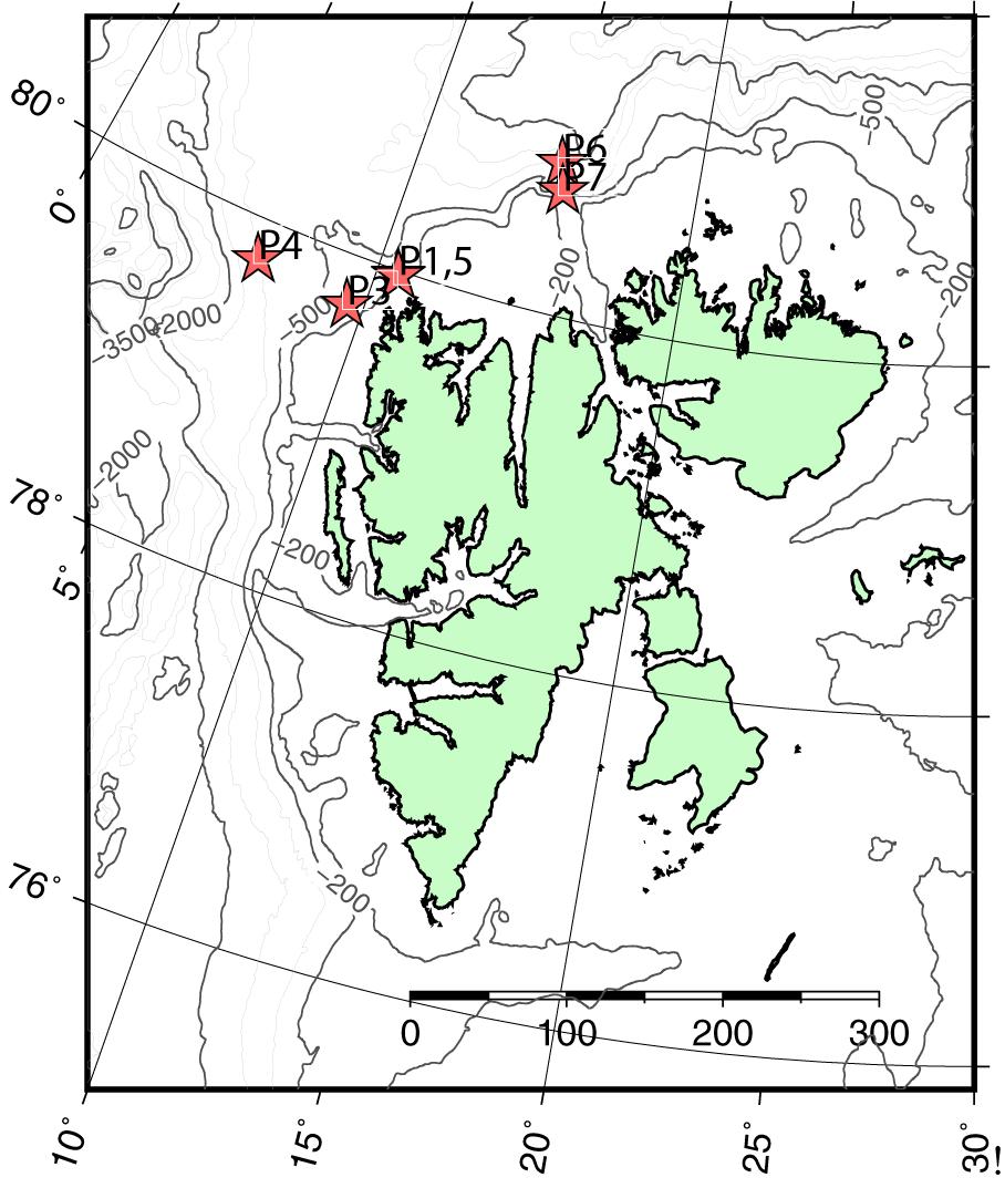
Figure 1. Chart of the research area around Svalbard, with sampling stations during the two cruises in May (P1–P4) and August (P5–P7). Locations of P1 and P5 coincide. P2 is missing due to lost moorings. Scale bar in km.

TABLE 1

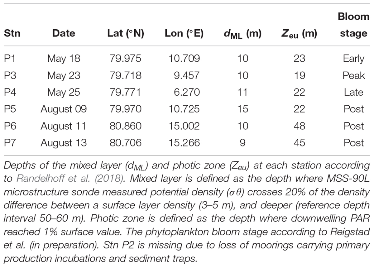
Table 1. Location of 24 h process stations in May and August 2014.

Vertical profiles of temperature, salinity and fluorescence were mapped with a rosette oceanographic profiler (CTD, Seabird SBE 911 plus). Water for analysis of carbon pools and biological process studies was retrieved with 5 L Niskin bottles from discrete depths (1, 5, 10, 20, 30, 40, 50, 75, 100, and 200 m), and the fluorescence maximum.

Carbon Pools

Total chlorophyll a (Chl a) samples (100–150 ml) were filtered onto Whatman GF/F glass-fiber filters (nominal pore of 0.7 μm). In addition, size fractionated Chl a (>10 μm, <3 μm) was obtained with membrane filters. Chl a was extracted in 5 ml of methanol at room temperature in the dark for 12 h without grinding. Triplicate samples of each size fraction were read with a Turner Fluorometer AU-10 (Holm-Hansen et al., 1965). Size-fractionated Chl a biomass was converted into phytoplankton carbon using a conversion factor of 27 (Riemann et al., 1989).

Total organic carbon (TOC) was measured from unfiltered seawater by high temperature combustion using a Shimadzu TOC-V_CSH. Samples were acidified with HCl (to a pH of around 2) and bubbled with N₂ gas in order to remove inorganic carbon. Particulate organic carbon (POC) samples were filtered in triplicate (100–500 ml) onto pre-combusted Whatman GF/F (450°C for 5 h), dried at 60°C for 24 h and analyzed on-shore with a Leeman Lab CEC 440 CHN analyzer after removal of carbonate with fumes of concentrated HCl for 24 h (Fischer and Wefer, 2013).

The concentration of dissolved organic carbon (DOC) was calculated from the difference of TOC and POC.

Heterotrophic bacteria (BAC) and heterotrophic nanoflagellates (HNF) were counted on an Attune^® Focusing Flow Cytometer (Applied Biosystems by Life Technologies) with a syringe-based fluidic system and a 20 mW 488 nm (blue) laser. Samples were fixed with glutaraldehyde (0.5% final conc.) at 4°C for a minimum of 2 h, shock frozen in liquid nitrogen, and stored at -80°C until analysis. For enumeration of bacteria the samples were diluted 10-fold with 0.2 μm filtered TE buffer (Tris 10 mM, EDTA 1 mM, pH 8), stained with a green fluorescent nucleic-acid dye, SYBR Green I (Molecular Probes Inc., Eugene, OR, United States) and kept for 10 min at 80°C. HNF samples were preserved in similar way, following staining with SYBR Green I (Molecular Probes Inc., Eugene, OR, United States) for 2 h in the dark, and minimum 1 ml was measured at a flow rate of 500 μl min^-1 (Zubkov et al., 2007). HNF were discriminated from nano-sized phytoplankton on basis of green vs. red fluorescence, and from large bacteria on basis of side scatter vs. green fluorescence. Abundances were converted to carbon biomass using a bacterial carbon content of 15 fg C cell^-1, and a HNF mean cell size of 33.5 μm³ and 20% carbon content (Børsheim and Bratbak, 1987; Ducklow, 2000).

Microzooplankton samples were preserved in 2% (final concentration) acid Lugol’s iodine, post-fixed with 1% (final concentration) formaldehyde after 24 h and stored at 4°C until counting. Microzooplankton were settled in Utermöhl chambers (50–100 ml) and counted under differential interference contrast (DIC) and fluorescence equipped inverted microscope. The entire chamber was scanned at 200× magnification. At least 40 individual cells within each abundant taxon were sized at 400–600× magnification and converted to carbon biomass according to geometric shapes and volume to carbon conversions (Menden-Deuer and Lessard, 2000). All ciliates, and hetero- and mixotrophic dinoflagellates > 20 μm in maximum dimension were allocated to microzooplankton.

Mesozooplankton composition, biomass, and depth distribution was assessed with net hauls from the bottom (or a maximum depth of 1,000 m at station deeper than 1,000 m) to the surface twice a day (noon and midnight). The vertically stratified samples (0–20, 20–50, 50–100, 100–200, 200–600, and 600–1,000 m) were collected with a MultiNet Midi (180 μm mesh size, 0.25 m² mouth opening, Hydro-Bios, Kiel, Germany) that was deployed vertically with a hauling speed of 0.5 m s^-1. Samples were preserved in a solution of 80% seawater and 20% fixation agent (75% formaldehyde buffered with hexamine, 25% anti-bactericide propandiol), resulting in a final formaldehyde concentration of 4% (for details see: Basedow et al., 2018).

From the fixed samples, zooplankton was counted and identified to the level of species (most copepods), genus or family (other groups). Conspicuous, large zooplankton (>5 mm, chaetognaths > 10 mm) were identified and enumerated from the entire sample. From the rest of the sample, at least 500 individuals from a minimum of three sub samples (2 ml, obtained with an automatic pipette with tip end cut to leave a 5 mm opening) were identified, staged and counted. This procedure allows for the analysis of abundance of common species and taxa with 10% precision and at 95% confidence level (Postel et al., 2000). Copepods of the genus Calanus were identified to species level (Kwasniewski, 2003). Specimens other than copepods were measured and sorted into different size categories. For the inverse reconstruction, mesozooplankton was aggregated into two size classes, small (<4 mm), and large (>4 mm). The latter also included the Calanus species (Calanus finmarchicus, Calanus glacialis, and Calanus hyperboreus). Mesozooplankton abundance was converted to carbon biomass by using species-specific conversion factors after an extensive compilation (E. Halvorsen, unpublished data) from a range of literature sources (e.g., Richter, 1994; Hanssen, 1997; Hirche and Kosobokova, 2003; Hopcroft et al., 2010), or a generic biovolume to carbon conversion factor of 0.03 mg C mm^-3 (Zhou et al., 2010).

Community Metabolic Rates

Algal ¹⁴CO₂ fixation was measured by the ¹⁴C method (Nielsen, 1952). Water samples from 1, 5, 10, 20, 30, 40, 50, and 75 m depth were split in 100 ml aliquots into four 150 ml polycarbonate bottles and spiked with 10 μCi of NaH¹⁴CO₃. One bottle served as a t₀ sample. One dark, and duplicate light bottles were incubated at in situ depths for ca 22 h, using a freely drifting or ice-floe attached mooring. Total ¹⁴CO₂ fixation, including organic exudates, was measured from a 2 ml sub-sample, and particulate ¹⁴CO₂ fixation from the remaining 98 ml Whatman GF/F filtered sample, placed in 6 ml scintillation vials. Residues of any inorganic ¹⁴C were removed by acidifying the samples with 0.2 ml of 20% HCl for 24 h. After acidification, 5 ml of Ultima Gold^TM XR LSC scintillation cocktail was added, and the samples stored in the dark until measuring on shore in a PerkinElmer Tri-Carb 2900TR scintillation counter. The activity in dark bottle was subtracted from the activities in the light bottles, and to assess dissolved primary production the particulate primary production was subtracted from the total. The detection limit was approximately 1 μg C L^-1 d^-1. In our study the ¹⁴CO₂ fixation rates were treated as gross primary production (GPP).

Bacterial production (BP) was measured using the radiolabeled leucine incorporation technique (Kirchman, 2001). Aliquots of 1.9 ml were incubated with ³H-leucine (final conc. 20 nmol L^-1; specific activity 5.957 TBq mmo L^-1) in the dark at 1°C for 2 h. Triplicate samples were taken from each profile depth, as well as one trichloroacetic acid (TCA) killed control (5% final concentration). The reaction was terminated by adding TCA (5% final concentration). Samples were microcentrifuged and aspirated. The remaining pellet was subsequently washed with TCA and ethanol. The samples were dried, and radio assayed with scintillation cocktail (Ultima Gold^TM XR LSC) with a PerkinElmer Tri-Carb 2900TR scintillation counter. Bacterial carbon production was calculated with a conversion factor 3.1 kg C mol 1 leucine incorporated (Simon and Azam, 1989).

Community respiration (ComResp) was determined from changes in oxygen over a 24 h period in 100 ml sample aliquots. Oxygen concentrations were analyzed by micro-Winkler titration using a potentiometric electrode and automated endpoint detection (Mettler Toledo, DL28 titrator) following Oudot et al. (1988). Community respiration was calculated by subtracting initial dissolved oxygen concentrations from dissolved oxygen concentrations measured after incubation in the dark. Due to the small aliquot volume, it was unlikely to contain any representative quantity of mesozooplankton. Therefore, the community respiration was not partitioned to mesozooplankton in the inverse reconstruction.

Vertical Particle Flux

To measure the vertical flux of organic particles (SED), we deployed a drifting, semi-Lagrangian array of sediment traps at eight depths (20, 30, 40, 50, 60, 90, 120, and 200 m). The array was free drifting or attached to an ice floe and was deployed for ca. 24 h. The sediment traps were parallel cylinders (7.2 cm in diameter, 45 cm height) mounted in a gimbaled frame equipped with a vain. At moderate current speeds, the cylinders remain vertical and perpendicular to the current direction. No baffles were used in the cylinders opening, and no fixatives were added to the traps prior to deployment. After recovery, the contents of the two replicate sediment trap cylinders were pooled into plastic bottles and kept cold and dark until processing for POC as described above.

Inverse Model Specification

To estimate the carbon flows between food web compartments with the linear inverse model (LIM), we need food web topology (matrix E), the measured compartment biomasses and rates of change therein (Δbiomass/Δt; vector f), and a set of quantitative constraints. The constraints can be directly measured by flows of the food web (hard constraints), or plausible physiological properties usually based on a literature search, which set the upper or lower bounds of flows (weak constraints). E.g., it is reasonable to consider all food web flows to be non-negative. The web topology (matrix E) describes the mass balances of the compartments, i.e., the flows of mass in and out of pre-defined compartments and is constructed based on our understanding of trophic relationships (who eats what). There are as many columns in matrix E as there are flows in the food web, and as many rows as there are compartments. The E matrix and f vector combined obey the conservation of mass principle, i.e., the compartment mass change equals to the sum of flows in, minus the sum of flows out of the compartment. Each compartment has its own mass balance equation, with unknown food web flow values. To solve the inverse problem, we need to find the unknown food web flows, forming a solution vector x, which simultaneously satisfies all the mass balances equations. In a matrix format the system of linear equations to be solved is:

$$E^{*}x=f$$

where matrix E is made of the coefficients in the mass balance equation, the solution vector x has a length equal to the number of columns in E, and the compartment mass change vector f has a length equal to the rows of E. Further, the solution vector has to satisfy a set of quantitative constraints. If some of the food web flows, or combination of flows, are measured from the food web under study (hard constraints), we constrain that flow, or combination of flows, to a particular value, which the solution vector has to satisfy. Each measured flow adds another equation to the system of linear equations. The solution vector also has to satisfy weak constraints (coefficients in matrix G), which set the upper or lower limits (vector h) to certain food web flows:

$$G^{*}x\ge h$$

E.g., food assimilation cannot be more than food intake by the organisms. Unlike more conventional modeling, which is a predictive tool to forecast changes in standing stocks form a set of deduced properties, inverse modeling does not predict, but inversely back-calculates the properties from observed data and plausible constraints.

In our study we grouped the pelagic food web components into 10 compartments, eight living and two non-living, for which mass balance equations were constructed (Supplementary Table S1). The eight living compartments of organism groups comprised the three size classes of autotrophs (PHY0, <3 μm; PHY1, 3–10 μm; PHY2, >10 μm, containing also the colonial Phaeocystis), heterotrophic bacteria (BAC), heterotrophic nanoflagellates enumerated with flow-cytometry (HNF), microzooplankton (μZOO), and two size classes of mesozooplankton (ZOO1, ZOO1; Table 2). The two non-living compartments were dissolved organic carbon (DOC) and detritus (DET, derived from measured POC minus the carbon biomass of living compartments). All compartments were expressed in units of organic carbon (mg C m^-3), and for the inverse reconstruction integrated to the upper 40 m layer (mg C m^-2). The upper 40 m layer included the surface mixed layer, and in most cases the euphotic layer (Table 1).

TABLE 2

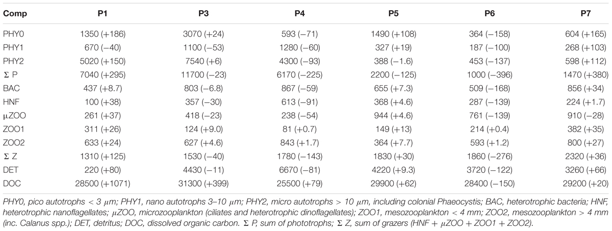
Table 2. Abbreviations of the planktonic food web compartments, the respective stock sizes (mg C m^-2) in the upper 40 m water column, and changes of stocks (mg C m^-2d^-1) in stations P1–P7.

The inverse model had three external flows: (i) primary production (GPP), fueling new organic carbon into the food web, and two flows by which carbon left the food web, (ii) respiration, and (iii) sedimentation of organic particles (SED). The model was driven by primary production, measured at each station, and integrated vertically to 40 m depth through trapezoidal integration (mg C m^-2 d^-1).

The measured community respiration (ComResp) was the sum of respiration by all living compartments (three size classes of phytoplankton, bacteria, heterotrophic nanoflagellates, and microzooplankton), with the exception of mesozooplankton. Community respiration measurements were conducted from the upper mixed layer, intermediate layer and chlorophyll maximum, and integrated vertically through trapezoidal integration (mg C m^-2 d^-1), assuming 1:1 ratio (O:C).

Sedimentation of organic particles was measured as POC (mg POC m^-2 d^-1) and partitioned by the food web model between three compartments: detritus (DET), large phytoplankton (PHY2), and mesozooplankton fecal pellets.

All three phototrophic compartments acquired CO₂ for photosynthesis, incorporated part of organic carbon as biomass (measured as particulate primary production), and exudated part of the organic carbon to the DOC pool (measured as dissolved primary production), and part of the carbon was respired back to CO₂. A fraction of the phototrophic biomass was lost to detritus through processes like mortality and lysis. Only the largest phytoplankton fraction (PHY2) contributed directly to sinking particles; smaller phytoplankton fractions contributed to vertical flux indirectly through detritus.

Bacteria took up DOC from the environment (bacterial assimilation), part of it was respired to CO₂, and part was incorporated into biomass (measured as net bacterial production). Bacterial biomass was lost to detritus through mortality. Viral lysis of bacteria can release significant amount of DOC also in high latitude marine environments (Chénard and Lauro, 2017), which is again taken up by the bacterial community. This viral loop and other causes of inter-bacterial DOC cycling are not dealt with explicitly here and are all incorporated into the bacterial compartment in our model.

Heterotrophic nanoflagellates and microzooplankton fed on smaller living compartments, microzooplankton also on detritus, and lost biomass through respiration to CO₂, exudation of organic matter to DOC, mortality to detritus, and through grazing by larger organisms. Microzooplankton, composed of heterotrophic dinoflagellates and ciliates in our study, are known grazers on Phaeocystis (Grattepanche et al., 2011; Swalethorp et al., 2019), but the grazing pressure depends on whether the prymnesiophyte is in its single-cell or colonial form (Grattepanche et al., 2011). Further, heterotrophic dinoflagellates are known to be voracious predators of large phytoplankton like other dinoflagellates and diatoms (Olseng et al., 2002; Jeong et al., 2004). We therefore allowed microzooplankton to prey on all size classes of phototrophs. We are also aware that several microzooplankton taxa could be mixotrophic, as kleptoplasty is common in both, dinoflagellates and ciliates (Gast et al., 2007; Stoecker et al., 2009), but these pathways are currently not considered in our model.

Mesozooplankton grazed on detritus and all other heterotrophic and phototrophic compartments except bacteria, picophototrophs, and large mesozooplankton also nano phototrophs. Mesozooplankton lost biomass through DOC release (sloppy feeding and other processes), respiration, and defecation. Part of the feces contributed directly to sinking particles, the other part disintegrated in the water column and contributed to the detritus pool (Wexels Riser et al., 2002). The detritus compartment gained biomass through mortality of all living compartments, and lost biomass to DOC through bacterial and chemical degradation, and through sedimentation.

The food web topology, showing all the linkages between compartments, is outlined in Figure 2. To narrow the allowable ranges for the reconstructed food web flows, we set an array of biologically relevant constraints (Supplementary Table S2). All flows were expected to be non-negative. The particulate and dissolved primary production was partitioned between the three phototrophic size classes according to the respective biomasses, but allowing for allometric negative scaling between cell size and mass-specific photosynthesis rate (Maraóón et al., 2007). We thus constrained the mass-specific primary production for smaller autotrophs to be larger than for the subsequent large autotroph compartment, but not more than two times larger. Autotrophic respiration was constrained to between 1 and 55% of the gross primary production (Falkowski et al., 1985). Phytoplankton mortality was assumed to be at least 1% of the biomass per day.

FIGURE 2

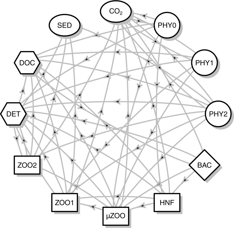
Figure 2. Food web topology of the linear inverse models. The same topology was used for all stations. Arrows represent carbon flows between compartments. Autotrophic compartments are in circle: PHY0, pico autotrophs < 3 μm; PHY1, nano autotrophs 3–10 μm; PHY2, micro autotrophs > 10 μm including colonial Phaeocystis. Diamond: BAC, heterotrophic bacteria; Heterotrophic grazers are in rectangles: HNF, heterotrophic nanoflagellates; μZOO, microzooplankton; ZOO1, small mesozooplankton < 4 mm; ZOO2, large mesozooplankton > 4 mm; Non-living organic compartments are in hexagons: DOC, dissolved organic carbon; DET, detritus. External compartments, with no mass balance equations, are in ellipses: SED, sedimentary carbon; CO₂, respired carbon.

For mesozooplankton we constrained the assimilation to be 40–80% of the food intake (Parsons et al., 2014). For other heterotrophic grazers (HNF, μZOO) the assimilation was assumed to be 80–90% of the food intake (Straile, 1997). Bacterial assimilation efficiency was assumed to be 100%. Respiration of the heterotrophic compartments was partitioned into a maintenance respiration, constrained between 1 and 10% of their respective biomass, and respiration associated with growth, which was constrained to be at least 40% of the assimilated food for eukaryotes (Sanders et al., 1992), or at least 10% for bacteria (del Giorgio and Cole, 1998).

Mesozooplankton DOC release (sloppy feeding, other processes) was constrained to be between 1 and 50% of the food intake (Møller et al., 2003; Møller, 2004). Mesozooplankton defecation was constrained between 10 and 60% of the food intake, and was further partitioned into a vertical particle flux of rapidly sinking fecal pellets, and disintegration within the water column into the detritus pool (Wexels Riser et al., 2002). Further, the fraction of sinking fecal pellets was set to be less than the flow to detritus pool, to be consistent with field observations form the Barents Sea (Wexels Riser et al., 2002). Microzooplankton and heterotrophic nanoflagellate exudation to DOC pool was constrained between 1 and 10% of food intake, and mortality between 1 and 10% of biomass per day. Bacterial daily mortality was set to be 1–10% of the bacterial biomass.

If heterotrophic grazers did not discriminate between food sources, the grazing rates would be proportional to the biomass of the respective prey items. We allowed preferential grazing and some discrimination between food sources, but not more than 0.5–2.0 times the respective prey biomass ratios. Further, we assumed that zooplankton grazers (μZOO, ZOO1, and ZOO2) feed on both, living compartments and detritus, but that they prefer living prey. Therefore, the grazing rates on detritus divided by the grazing rates on live compartments was set lower than the biomass ratio of detritus to live prey compartments.

In summary, the inverse food web model had 10 compartments with mass balances (eight living, two non-living; Figure 2 and Supplementary Table S1), five measured flows (community respiration, particulate and dissolved primary productions, bacterial net production, vertical flux of organic particles), 48 reconstructed food web flows (Figure 2 and Supplementary Table S3), and 85 biological constraints (Supplementary Table S2). The inverse reconstruction was run with the LIM library of the R software (van Oevelen et al., 2010). The food web architecture and biological constraints were kept constant throughout the study and were applied for each individual data set from stations P1–P7. With 15 equations (10 mass balances plus 5 measured flows) and 48 unknown flows (rank parameter equal to 15), the system was under-determined and had infinite number of solutions, which satisfy the equations. A sensible choice is to follow the principle of parsimony, picking a solution with the minimum norm, i.e., the solution with the lowest sum of squared flow values.

However, this minimum norm solution is not based on ecological theory nor supported by empirical evidence. Further, it tends to push some of the flows to the lower bounds of their possible ranges, which should be considered extreme rather than likely values (Kones et al., 2006). We therefore opted here for the alternative likelihood approach, which considers all the possible solutions of the food web by sampling the probability density function (PDF) of LIM solution space by using a Markov Chain Monte Carlo algorithm (Meersche et al., 2009). This approach has an interesting useful property: although the PDF of the LIM domain is uniform, emphasizing that all valid solutions are equally likely, the marginal probability density function (mPDF) of an individual flow is not uniform. This is because mPDF integrates over the valid areas of all other flows and therefore some selections within the individual flow range render as more likely (van Oevelen et al., 2010). We fed the xsample() function with initial minimum norm solution [obtained with function lsei()] as an initial starting set and sampled the LIM solution space with 10,000 MCMC random draws. The xsample() MCMC algorithm uses a symmetrical random jump function that only depends on the previously accepted point to draw a new sample. Each of the realizations corresponds to an equally likely solution vector x of the food web flows, which obeys the mass balances, as well as the data and constraints. Here we summarize the likelihood of each individual flow as the mean (±SD) of the sampled mPDF.

The mass balance equations are usually balanced with rates of change of the compartment biomasses, measured over a period of time (e.g., Forest et al., 2011). In our 24 h process stations no sensible time series was feasible, leaving us with an alternative to assume a steady state food web and consider the rates of biomass change to be zero. However, our measured boundary input flows (primary production) were not balanced by output boundary flows (community respiration plus sedimentation), thus rendering a steady state problem infeasible, unless we introduce new ad hoc export or advection functions. To balance the system, we relaxed the steady state assumption, and defined the compartment mass balances as approximate, not as exact equations in the inverse analysis lsei() function, which then resolved the biomass changes in the minimum norm sense. This initial minimum norm solution was then inserted as the starting set to the xsample() function (see above).

Results

Measured Biomasses

The measured organic carbon masses of the living and non-living compartments, and their reconstructed rates of change, are given in Table 2. The raw vertical profiles of biomasses and flows are presented in Supplementary Figures S1–S5. The largest organic carbon pool was in the dissolved fraction (25–31 g C m^-2). DOC exceeded the particulate carbon pool generally by a factor of 3–4, but only by a factor of 1.6–1.7 during the peak and decline phases of the algal bloom (P3 and P4).

The partitioning of the particulate organic carbon revealed a conspicuous and rapid shift from phytoplankton to detritus domination, as the season progressed (Figure 3). The early bloom stage had a very low detritus biomass (ca 0.2 g C m^-2), but a substantial phytoplankton biomass (>7 g C m^-2), mostly in the larger micro fraction (5 g C m^-2). By the peak of the bloom the phytoplankton biomass had increased further (up to ca 12 g C m^-2; mainly in the micro and pico fractions), but there was also a substantial build-up of detritus (up to 4.4 g C m^-2). By the late bloom stage, the detritus biomass reached its peak (ca. 6.7 g C m^-2), while the phytoplankton was on decline (6.2 g C m^-2). The bloom progression in May followed a shift from Phaeocystis pouchetii dominance to a co-dominance with guild of diatoms from the genera Chaetoceros (Chaetoceros socialis, Chaetoceros holsaticus, and Chaetoceros furcellatus), Thalassiosira (Thalassiosira hyaline and Thalassiosira nordenskioldii), Fragillariopsis (Fragillariopsis oceanica and Fragillariopsis furcellatus), and the presence of medium-sized dinoflagellates from the genera Gymnodinium and Protoperidinium. The post bloom stages in August had only a modest phytoplankton biomass (1–2 g C m^-2), but the detritus remained high (3.2–4.2 g C m^-2). Overall the percentage of detritus from POC increased from 2.4 to 24% to 43%, as the bloom progressed in May and varied between 41 and 52% in August. The dominant phytoplankton groups in August were small flagellates, coccolithophorids, cryptophytes, (Teleaulax) chrysophytes (Dinobryon), chlorophytes (Pyraminonas), dinoflagellated (Gymnodinium and Oxyrrhis), but also some diatoms and Phaeocystis pouchetii.

FIGURE 3

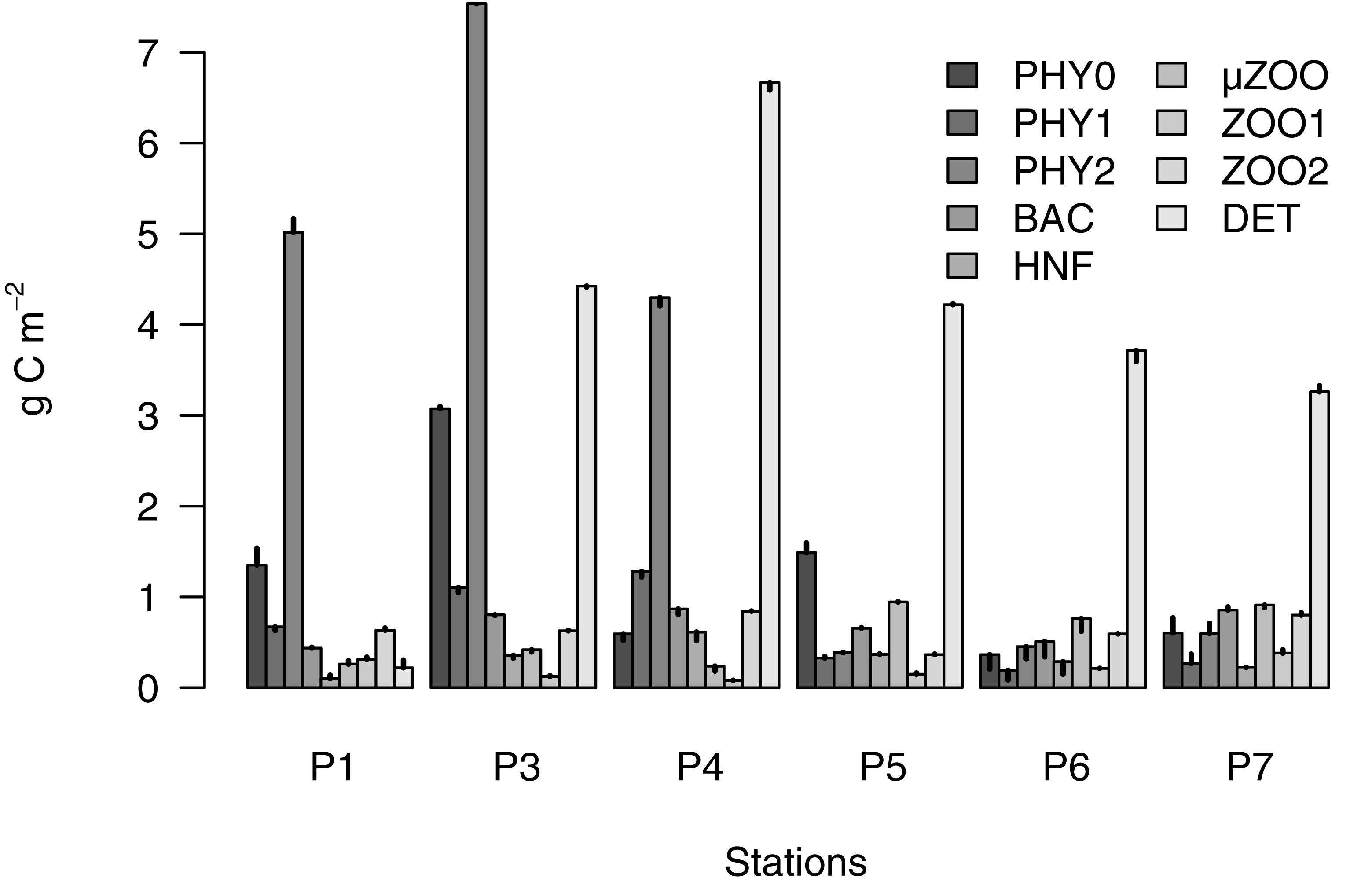
Figure 3. Biomass of the measured particulate food web compartments in the upper 40 m water column of stations P1–P7. The error bars show the daily rate of change of the biomass (g C m^-2 d^-1), as estimated by the inverse solution.

The lower food web components followed the evolution of the successional stages (Table 2). Bacterial biomass doubled from the early to peak and late bloom phases (from 440 to 870 mg C m^-2) and remained high during the post bloom stages (510–860 mg C m^-2). Heterotrophic nanoflagellates revealed a rapid biomass increase from early to late bloom (100–610 mg C m^-2) and retained a modest biomass during post bloom stages (220–370 mg C m^-2). Microzooplankton retained low biomass during all the bloom stages (240–420 mg C m^-2) but increased notably during the post bloom stages (760–940 mg C m^-2). Mesozooplankton biomass reveled no discernible pattern related to the successional stages, and varied between 80–380 mg C m^-2, and 360–840 mg C m^-2, for the small and large fractions, respectively.

External Flows

The measured external flows were the gross primary production (GPP) into the system, and two competing flows out of the system, respiration and sedimentation. GPP decreased from 2.85 to 1.33 to 0.65 g C m^-2 d^-1 and varied between 0.29 and 1 g C m^-2 d^-1, during the post bloom phases (Figure 4).

FIGURE 4

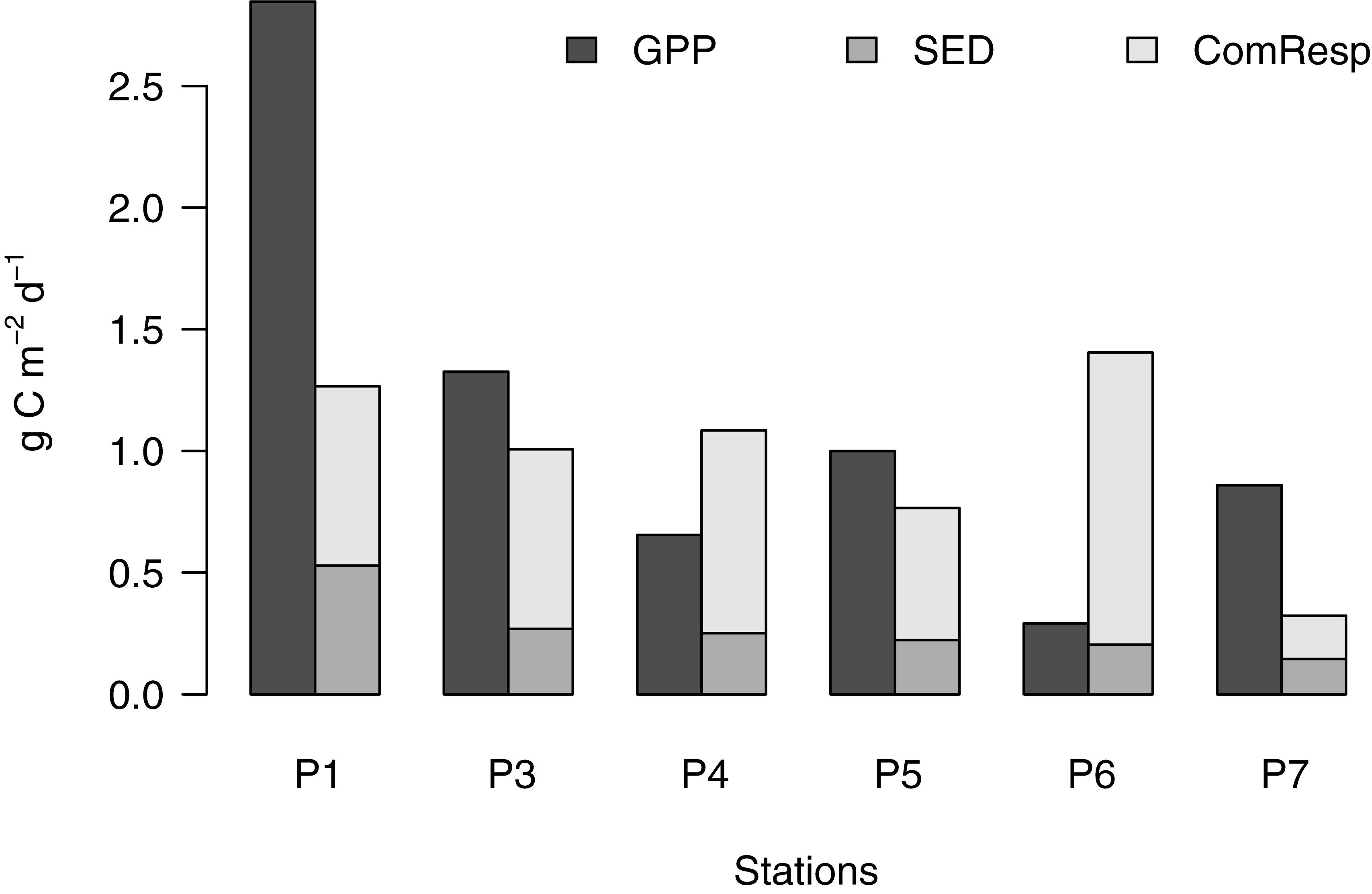
Figure 4. External flows into the food web, gross primary production (GPP), and two loss rates: the vertical flux of particles (SED), and community respiration (ComResp). Whenever GPP exceeds the sum of SED and ComResp, the food web is increasing in mass, and vice versa.

Respiration always exceeded the sedimentation losses (Figure 4), indicating the relative efficiency of the food web in retaining energy resources. The inverse reconstruction partitioned the majority of the community respiration during the pre-bloom phase to bacteria (500 mg C m^-2 d^-1, corresponding to 68% of the community respiration), but the rate and proportion decreased rapidly as the bloom progressed (to 50 and 33% at peak and late bloom stages, respectively). Concomitantly, the respiration of the phototrophic compartments increased from 9% during the pre-bloom state to >16% thereafter, and the sum of grazer respiration from 23 to >60% as the community maturated during late and post bloom stages (Figure 5).

FIGURE 5

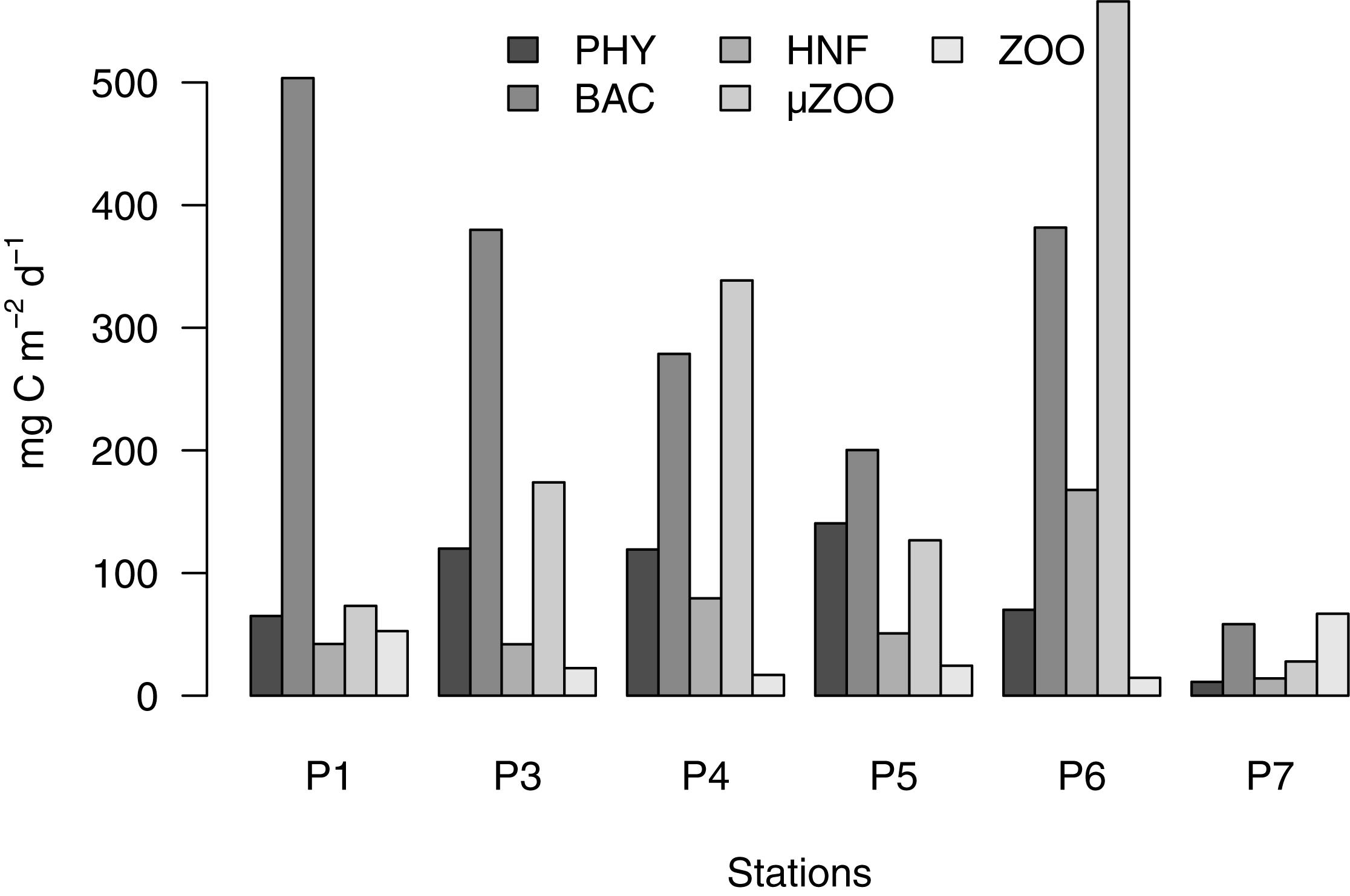
Figure 5. Partitioning of the community respiration flows. Note that all phototrophs and pooled into PHY, and the two mesozooplankton size classes into ZOO.

Sedimentation was relatively higher (251–529 mg C m^-2 d^-1) during the bloom stage in May, and 145–223 mg C m^-2 d^-1 in August. The vertical flux of organic particles increased from 19 to 20 to 38% of the GPP during the early, peak, and late bloom phases in May, and varied between low values of 17% (P5) to as high as 70% (P7) during post bloom phases. Overall, sedimentation losses were 5.8% of the total particulate carbon standing stock during the early bloom stage, and only <3% thereafter. The vertical flux of organic particles was predominantly partitioned between detritus (56–85%) and phytoplankton (11–36%), while zooplankton fecal pellets contributed a minor fraction (Figure 6).

FIGURE 6

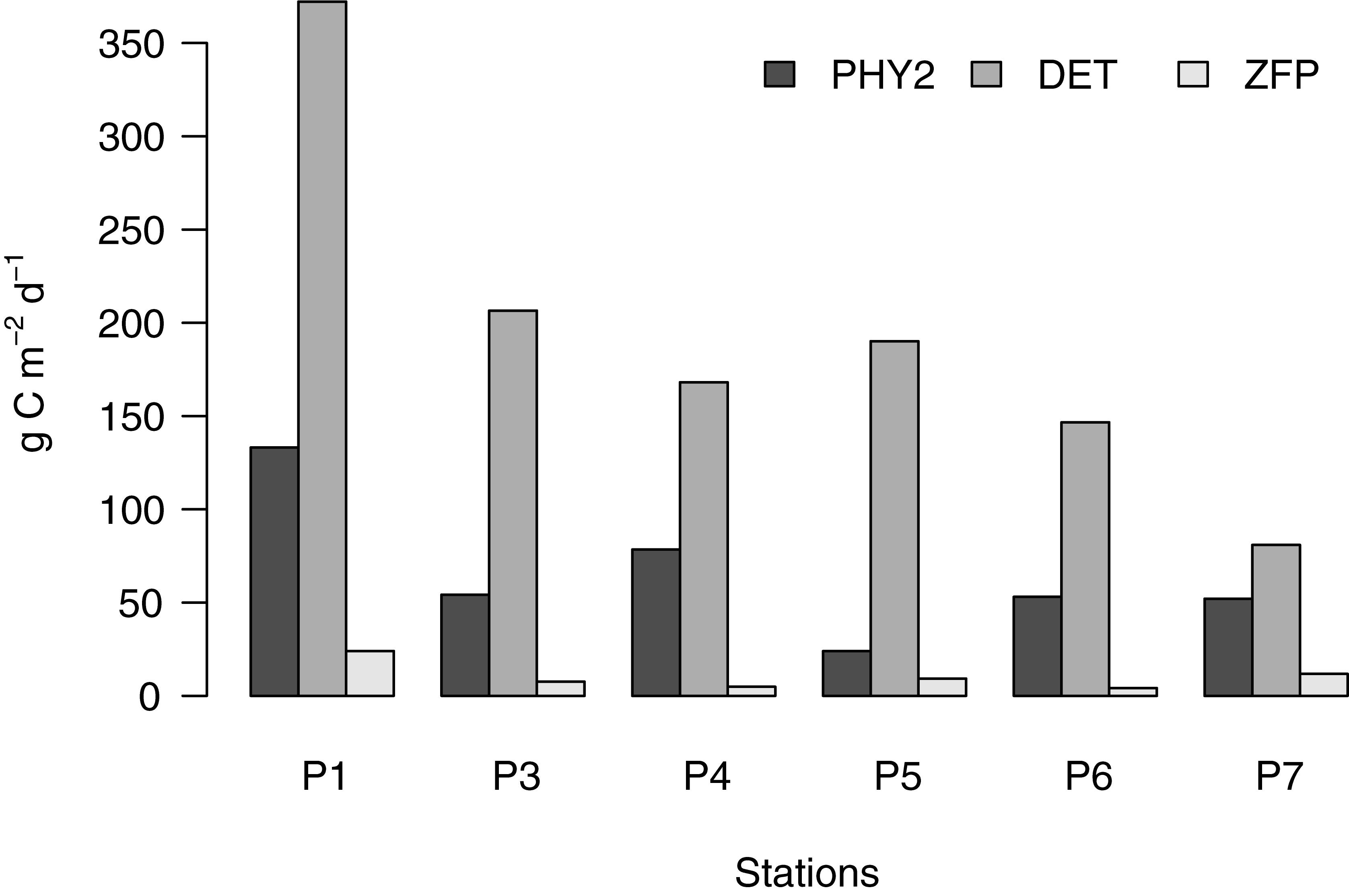
Figure 6. Partitioning of the vertical flux of organic particles. ZFP denoted direct vertical flux of fecal pellet carbon combined from both mesozooplankton size classes.

The difference between the carbon flows in and out of the system shows the growth or shrinkage of the food web. Figure 4 shows the sum of the external flows, indicating a rapid growth of the system mass during the early bloom phase, where GPP exceeded the sum of respiration and sedimentation losses by 1.6 g C m^-2 d^-1. This increase of the food web continued during the peak bloom phase at a slower pace (0.3 g C m^-2 d^-1) and turned into system shrinkage at the late stage of the bloom (-0.4 g C m^-2 d^-1). The post bloom stages showed variation in both directions (Figure 4). The food web turned net heterotrophic during the bloom decline phase, and in station P6 during the post bloom stage, where GPP was 78 and 24% of community respiration, respectively.

Reconstructed Internal Food Web Flows

The internal flow pattern was dominated by two flows, exudation by phytoplankton into the DOC pool, and bacterial assimilation of DOC (Figure 7 and Supplementary Table S3). Phytoplankton exudation varied by more than an order of magnitude and was highest during the early bloom stage (1565 mg C m^-2 d^-1), dropped rapidly thereafter to 620 mg C m^-2 d^-1 during the peak bloom, and to 205 mg C m^-2 d^-1 and below in late and post bloom stages. Phytoplankton exudation formed a decreasing proportion, from 55 to 49 to 31%, of the GPP during the bloom stages in May. During the post bloom stages in August the dissolved fraction of GPP was generally low, 9–12% (P5 and P7), and 26%, in P6. The other significant source of DOC was dissolution from detritus (up to 170 mg C m^-2 d^-1), which formed 1.6 to 4.6% of the detritus biomass, and 20 to 56% of the total food web DOC release (apart from the negligible <1% during the early bloom stage). Heterotrophic grazers contributed little to the DOC pool (20–51 mg C m^-2 d^-1), which formed 2–18% of the total food web DOC release.

FIGURE 7

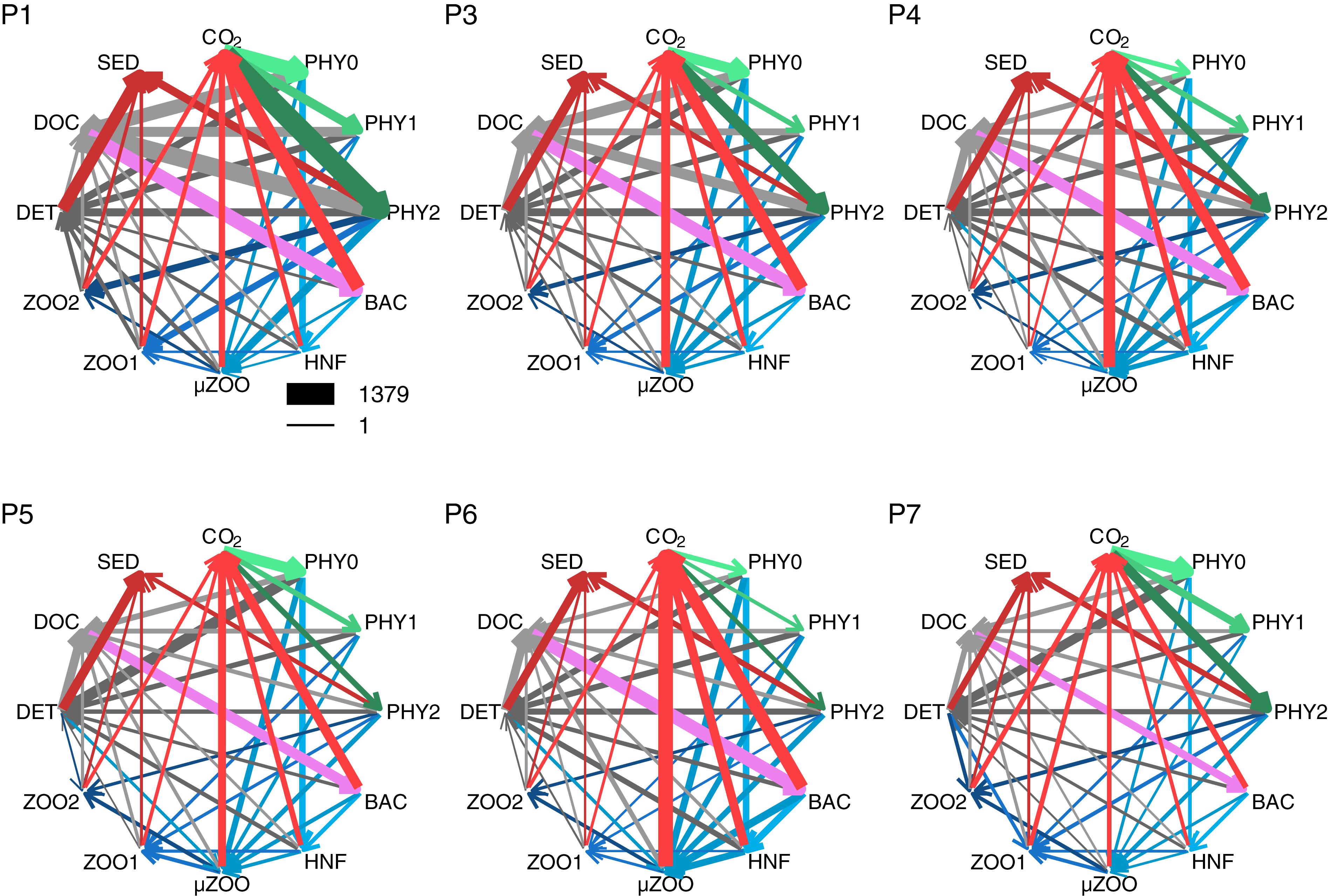
Figure 7. The carbon flows in stations P1–P7, as reconstructed from the field measurements by the inverse method (numerical values in Supplementary Table S3). The thickness of arrows is proportional to the square root of the respective flows, and have the same scale in all plots, as indicated by the legend (mg C m^-2 d^-1). Note the very low primary production in P6. Phototrophic flows are in green, carbon losses to SED and CO₂ are in red, grazing flows are blue, bacterial assimilation violet, and flows to non-living organic compartments, DOC and DET, are in gray.

Bacterial assimilation was highest during the early and peak bloom stages, 535 and 406 mg C m^-2 d^-1, respectively, and decreased thereafter to 329 mg C m^-2 d^-1 and below (except 439 mg C m^-2 d^-1 in station P6). Bacterial assimilation was in correspondence with the rate of fresh DOC production, but statistically not significantly (Pearson r = 0.77, p = 0.07, n = 6).

Other internal flows were related to grazing by the zooplankton compartments (collectively 240–664 mg C m^-2 d^-1), as well as zooplankton mortality and defecation (up to 52 mg C m^-2 d^-1). Detritus formation was relatively stable (401–468 mg C m^-2 d^-1) during the bloom phases in May, and somewhat more variable in August (331–498 mg C m^-2 d^-1). The percentage of GPP channeled to detritus increased from 16 to 31% to 61% during the bloom progression in May and varied from 38% (P7) to 147% (P6) in August. The sources and sinks of detritus were approximately balanced, when averaged over all stations. The ratio between the sum of sources and sinks of detritus varied between 1.25 and 0.78 (mean 1.01 ± 0.19). On average half of the detritus (194 ± 98 mg C m^-2 d^-1) settled out of the water column, the other half was almost equally partitioned between dissolution (119 ± 70 mg C m^-2 d^-1) and grazing (119 ± 81 mg C m^-2 d^-1). On average, microzooplankton was the main detrivorous group (86 mg C m^-2 d^-1; 62% of detrivory), followed by large (18 mg C m^-2 d^-1; 21%) and small (14 mg C m^-2 d^-1; 17%) mesozooplankton.

Sensitivity Analysis

To increase confidence in the model, we analyzed the robustness of the reconstructed fluxes to changes in the 10 measured compartment biomasses and the five measured flows. The sensitivity analysis was done by perturbing each measured input at a time by ±10%, while keeping other variables unchanged. The six stations and fifteen input variables, each increased and decreased by 10%, resulted in 180 perturbed food web models and 178 successful solutions. Most flow values changed somewhat after perturbation. For each solution we calculated the absolute sum of these changes. The sum of absolute flow changes, as percentage of the sum of flows in the original unperturbed system was calculated as a variation index for each of the input variable. We used both, the minimum norm, and the likelihood approaches to test the model sensitivity. Both methods gave similar results and for consistency we here present the likelihood approach.

Sensitivity analysis shows that the variation index always remained below 10%, regardless of the input variable perturbed (Figure 8). Nevertheless, the overall sensitivity of the reconstructions depended on which input variable was perturbed. Firstly, the inverse solutions tended to be less sensitive to perturbations in the standing stock biomass estimates (PHY0, PHY1, …, DOC), and more sensitive to boundary condition rate measurements (SED, ComResp, and GPP). The high variability within the individual effects (1–7%; Figure 8) indicated that the food web sensitivity during different stages of the bloom development also varied considerably. In summary, our sensitivity analysis indicates that small systematic errors in the input data would not affect the inverse solution in a disproportionate manner.

FIGURE 8

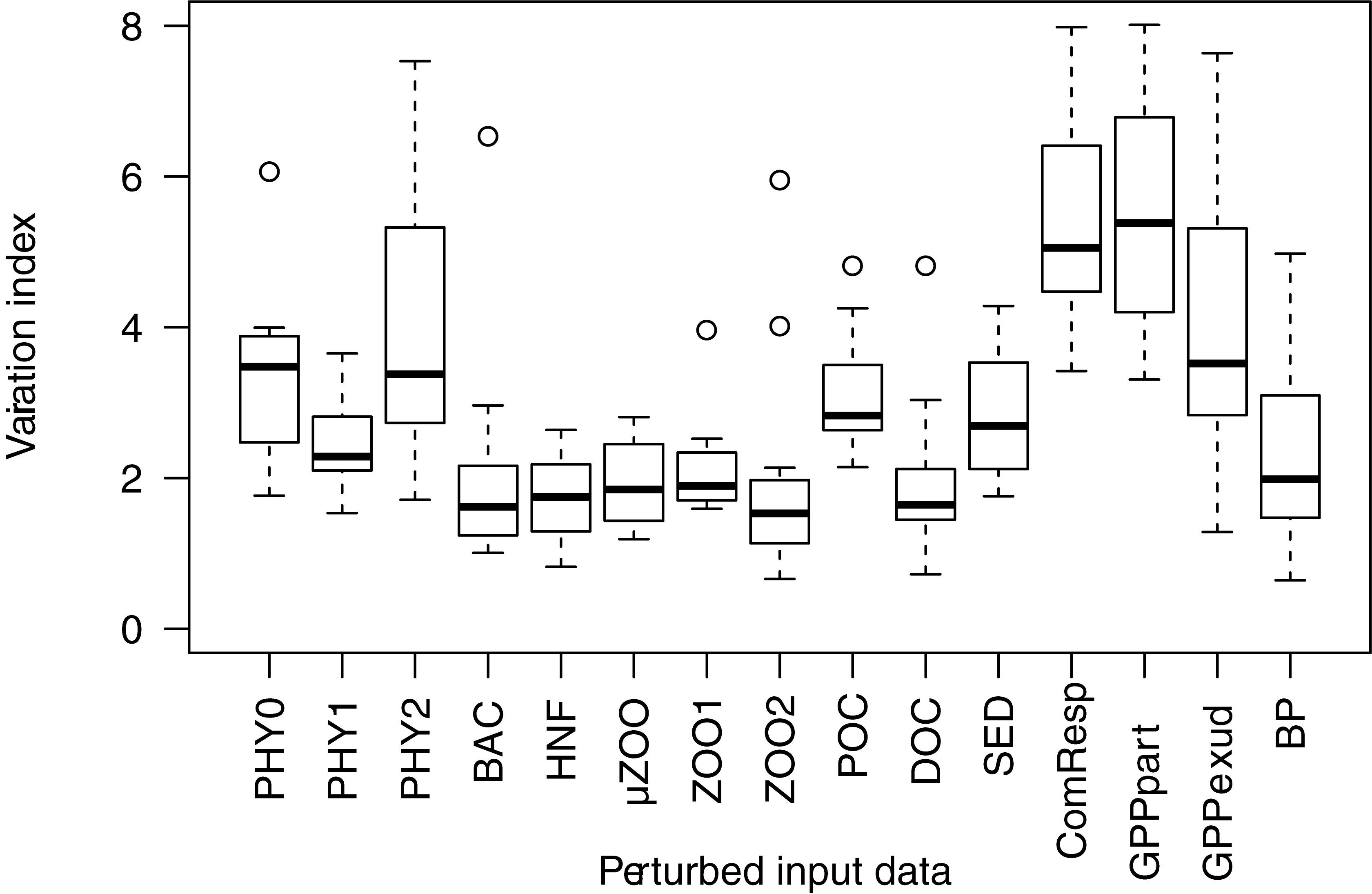
Figure 8. Sensitivity analysis. The boxplots show the spread in the variation index over stations P1–P7. Variation index is calculated as the sum of absolute reconstructed flow changes after perturbing each input variable (x-axis) at a time and divided by the sum of flows in the unperturbed food web. SED, vertical flux of organic particles; ComResp, measured community respiration; GPPpart, particulate GPP; GPPexud, dissolved GPP; BP, net bacterial production; other x-axis abbreviations as in Table 2.

Discussion

The seasonal stages and community maturation were reflected in the considerable diversity of the food web flows, even though the structural assumptions of the food webs were kept constant. The over-arching commonality was the dissolved fraction as the largest organic carbon pool. Only during the peak and decline phases of the algal bloom did the substantial build-up of phytoplankton and detritus, respectively, result in relatively lower difference between the dissolved and particulate organic carbon pools.

The input and consumption of DOC revealed considerable seasonal variation. The food web DOC release decreased rapidly during the bloom in May (from 1572 to 275 mg C m^-2 d^-1) and remained modest during post-bloom stages (<200 mg C m^-2 d^-1). Presumably the large input in spring was due to the predominance of colonial Phaeocysts during the bloom phase, which is known to produce conspicuous amounts of extracellular polysaccharides (Billen and Fontigny, 1987; Verity et al., 2007; Thornton, 2014). The released DOC was readily assimilated by bacteria (122–534 mg C m^-2 d^-1), but at a high respiration cost (200–504 mg C m^-2 d^-1; but in P7 only 58 mg C m^-2 d^-1). This led to a substantial seasonal dynamics of bacterial growth efficiency, from low values of 6% during the early and peak bloom phases to 16% at the bloom decline phase. The bacterial growth efficiency was variable, 22, 13, and 53%, during the post bloom stages. These values are within the range of literature reports from various oceanic systems (del Giorgio and Cole, 1998, and references therein). Our evidence thus points that the blooms of colonial Phaeocystis are a fresh source of DOC, but the quality of this substrate, low in nitrogen compounds, is low for bacterial consumption (Billen and Fontigny, 1987; Carlson et al., 1999; Williams et al., 2016), and the assimilation by the ambient assemblages has a high energetic cost. Further, bacteria consumed only 33–50% of the freshly released DOC during the early and peak bloom phases, but as much as 81% during the decline bloom phase. During the post-bloom stages in August the bacterial carbon assimilation matched fairly closely the instantaneous DOC release (80–86% in P5 and P7) or even exceeded it (152% in P6).

The seasonality, driven by the phytoplankton production and DOC release, cascaded through the food web, being more clearly expressed at the lower part of the food web. The seasonality in fresh DOC release was clearly discernible in bacterial biomass accumulation, which almost doubled from 437 mg C m^-2 at pre-bloom stage to 803 and 866 mg C m^-2 at peak and late bloom stages, a hallmark of Phaeocystis bloom associated bacterial activity (Billen and Fontigny, 1987). There was thus a time lag between the high DOC release at the early bloom stage, and the bacterial production and biomass response, further supporting only modest degradability of the Phaeocystis exudates (Carlson et al., 1999; Williams et al., 2016). Also, heterotrophic nanoflagellates revealed a very rapid biomass build up from 100 to 613 mg C m^-2 during the course of the bloom, suggesting a swift response to the increased resource availability. In contrast, microzooplankton, composed of large protists in our model, revealed only broad seasonal shifts in biomass between May and August, uncoupled from the dynamics of the bloom. The trophic cascade signal become indiscernible in the response of mesozooplankton compartments.

Another conspicuous seasonal feature was a shift from a system, where the POC pool was dominated by phytoplankton during the early bloom stage, to a system dominated by detritus. This indicates that during the polar winter the water column comes to be low in organic particles, and the new seasonal build-up of POC is initiated by phytoplankton. The rapid build-up of detritus during the early, peak, and decline phases of the bloom, from 220 to 4425 to 6667 mg C m^-2 were in line with a substantial mortality loss of phytoplankton (240–347 mg C m^-2 d^-1) already at an early seasonal stage of the community maturation.

The conspicuous shift in organic particle composition from phytoplankton to detritus dominance had a profound effect on zooplankton feeding. Mesozooplankton herbivory decreased from 92 to 78% to 69% of food intake during the bloom progression and was only between 20 and 28% during post bloom stages. During the post bloom stages the drop in herbivory was compensated by detritivory (27–62% of food intake), and carnivory (consumption of HNF and microzooplankton; 17–45% of food intake). The pattern was paralleled by microzooplankton, with rapid drop of herbivory from 97 to 72% to 45% during the bloom progression and staying at that level (32–55%) during the post bloom stages in August. The microzooplankton diet changed predominantly to detritus (27–43% of food intake), with carnivory (4–15%) and bacterivory (7–18%) of lower importance in August. The available evidence thus supports a flexible omnivorous feeding behavior of the dominant zooplankton groups, which is in line with recent studies from the Arctic (Forest et al., 2011; Vernet et al., 2017).

Community respiration was 26, 55, and 126% of GPP in the early, peak, and late bloom stages, indicating switching from net-phototrophy to net-heterotrophy as the spring bloom maturated. During the post-bloom stages, the ratio of community respiration to GPP varied even more, from 21% (P7) to 410% (P6), suggesting high spatial heterogeneity in the physical water mass as well as food webs properties over relatively short distances.

Due to the logistical reasons, compartment biomasses were measured only once per station, and rates of mass change were only approximated by the inverse analysis (Figure 3). Summing up the changes in particulate pools, i.e., the living compartments and detritus, gave the rate of mass change of the particulate organic carbon pool. As expected, there was a strong particulate biomass build-up during the early bloom phase (509 mg C m^-2 d^-1), which turned into a biomass decrease already during the peak (-80 mg C m^-2 d^-1), and even more so during the bloom decline phase (-509 mg C m^-2 d^-1). During the post-bloom stages, the biomass change rates varied even more, from 516 mg C m^-2 d^-1 (P7) to -962 mg C m^-2 d^-1 (P6), underlining the high heterogeneity of water masses in close spatial proximity in the Arctic marginal ice zone. The rate of biomass change divided by the GPP indicates the efficiency of the food web to convert primary production to particulate matter. The ratio was relatively low, 0.18, during the early bloom phase, and the positive values during post bloom stages ranged from 0.17 (P5) to 0.6 (P7).

The sum of grazing flows by heterotrophic nanoflagellates, micro- and mesozooplankton ranged from 268 to 834 mg C m^-2 d^-1, with no clear seasonal pattern. The total grazing pressure increased from 17 to 27 to 77% of GPP, as the bloom progressed in May. In August the grazing pressure was 31–44%, except in P6, where it was exceptionally high (286%). This suggests that the high gross primary production during a Phaeocystis dominated bloom does not support a high carbon turnover in the grazing food web. This is in line with the poor usability of Phaeocystis derived dissolved organic carbon by heterotrophic bacteria.

Partitioning the carbon turnover by heterotrophic grazers revealed high variability, an increasing role of microzooplankton during the bloom progression in May, and approximately equal mean apportionment between the two size classes of mesozooplankton (Figure 9). Averaging the carbon intake over all the six stations revealed microzooplankton as the most important grazer group (279 ± 202 mg C m^-2 d^-1), followed by the sum of the two mesozooplankton compartments (113 ± 76 mg C m^-2 d^-1), and heterotrophic nanoflagellates (87 ± 49 mg C m^-2 d^-1). Microzooplankton has been recognized as a main grazer compartment globally, estimated to consume over half of the daily global planktonic primary production (Calbet and Landry, 2004; Schmoker et al., 2013). Further, several specialized microzooplankton taxa, like the heterotrophic Gymnodinium and Gyrodinium species, and tintinnid ciliates, are known to pray upon Phaeocystis cells (Grattepanche et al., 2011; Swalethorp et al., 2019). This takes place particularly in the late bloom stage, when single cells are often released from colonies possibly when nutrients become limited (Jakobsen and Tang, 2002; Nejstgaard et al., 2007).

FIGURE 9

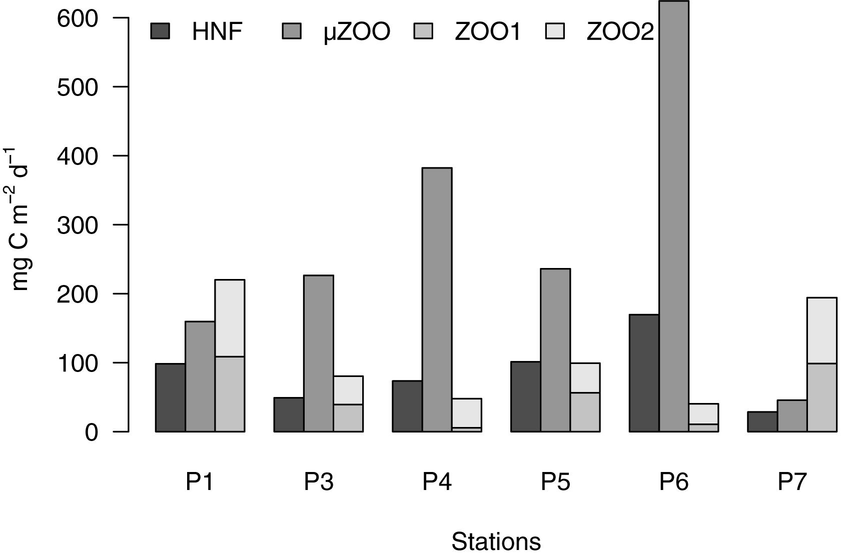
Figure 9. Partitioning of sum of grazing flows into the main heterotrophic grazer compartments. The mesozooplankton compartments are stacked to give the total carbon flow into mesozooplankton.

Author Contributions

KO participated in the cruises, designed the study, conducted the model analysis, and was in charge of the writing. EH, MV, PL, GF, MS-M, MP, and MR provided data for the model, participated in food web construction, data interpretation and writing. EH provided all the mesozooplankton data and searched or measured the values for mesozooplankton carbon content. MV provided data on particulate and dissolved primary production. PL and GF contributed with the microzooplankton data. MS-M provided the data for community respiration. MP provided data for microbial components and TOC. MR organized the cruise, was in charge of the project, and provided the data for chlorophyll, POC, and vertical flux.

Funding

This work was funded by the Estonian Research Council (Grant 1574P), and the Norwegian Research Council through the project CarbonBridge (Project Number 226415).

Conflict of Interest Statement

The authors declare that the research was conducted in the absence of any commercial or financial relationships that could be construed as a potential conflict of interest.

Acknowledgments

We thank the captain and crew of the R/V Helmer Hanssen for their helpful cooperation.

Supplementary Material

The Supplementary Material for this article can be found online at: https://www.frontiersin.org/articles/10.3389/fmars.2019.00244/full#supplementary-material

References

Arrigo, K. R., and van Dijken, G. L. (2015). Continued increases in Arctic Ocean primary production. Prog. Oceanogr. 136, 60–70. doi: 10.1016/j.pocean.2015.05.002

CrossRef Full Text | Google Scholar

Basedow, S. L., Sundfjord, A., von Appen, W.-J., Halvorsen, E., Kwasniewski, S., and Reigstad, M. (2018). Seasonal variation in transport of zooplankton into the arctic basin through the atlantic gateway. Fram. Strait. Front. Mar. Sci. 5:194. doi: 10.3389/fmars.2018.00194

CrossRef Full Text | Google Scholar

Beszczynska-Moller, A., Fahrbach, E., Schauer, U., and Hansen, E. (2012). Variability in Atlantic water temperature and transport at the entrance to the Arctic Ocean, 1997-2010. ICES J. Mar. Sci. 69, 852–863. doi: 10.1093/icesjms/fss056

CrossRef Full Text | Google Scholar

Billen, G., and Fontigny, A. (1987). Dynamics of a phaeocystis-dominated spring bloom in Belgian coastal waters. II. Bacterioplankton dynamics. Mar. Ecol. Prog. Ser. 37, 249–257. doi: 10.3354/meps037249

CrossRef Full Text | Google Scholar

Blais, M., Ardyna, M., Gosselin, M., Dumont, D., Bélanger, S., Tremblay, J. É., et al. (2017). Contrasting interannual changes in phytoplankton productivity and community structure in the coastal canadian arctic ocean: variability in arctic phytoplankton dynamics. Limnol. Oceanogr. 62, 2480–2497. doi: 10.1002/lno.10581

CrossRef Full Text | Google Scholar

Børsheim, K., and Bratbak, G. (1987). Cell volume to cell carbon conversion factors for a bacterivorous Monas sp. enriched from seawater. Mar. Ecol. Prog. Ser. 36, 171–175. doi: 10.3354/meps036171

CrossRef Full Text | Google Scholar

Calbet, A., and Landry, M. R. (2004). Phytoplankton growth, microzooplankton grazing, and carbon cycling in marine systems. Limnol. Oceanogr. 49, 51–57. doi: 10.4319/lo.2004.49.1.0051

CrossRef Full Text | Google Scholar

Carlson, C., Bates, N., Ducklow, H., and Hansell, D. (1999). Estimation of bacterial respiration and growth efficiency in the Ross Sea, Antarctica. Aquat. Microb. Ecol. 19, 229–244. doi: 10.3354/ame019229

CrossRef Full Text | Google Scholar

Chan, F. T., Stanislawczyk, K., Sneekes, A. C., Dvoretsky, A., Gollasch, S., Minchin, D., et al. (2018). Climate change opens new frontiers for marine species in the Arctic: current trends and future invasion risks. Glob. Chang. Biol. 25, 25–38. doi: 10.1111/gcb.14469

PubMed Abstract | CrossRef Full Text | Google Scholar

Chénard, C., and Lauro, F. M. (2017). “Exploring the viral ecology of high latitude aquatic systems,” in Microbial Ecology of Extreme Environments, eds C. Chénard and F. M. Lauro (Cham: Springer International Publishing), 185–200. doi: 10.1007/978-3-319-51686-8_8

CrossRef Full Text | Google Scholar

De Laender, F., Soetaert, K., and Middelburg, J. J. (2010). Inferring chemical effects on carbon flows in aquatic food webs: methodology and case study. Environ. Pollut. 158, 1775–1782. doi: 10.1016/j.envpol.2009.11.009

PubMed Abstract | CrossRef Full Text | Google Scholar

del Giorgio, P. A., and Cole, J. J. (1998). Bacterial growth efficiency in natural aquatic systems. Annu. Rev. Ecol. Syst. 29, 503–541. doi: 10.1146/annurev.ecolsys.29.1.503

CrossRef Full Text | Google Scholar

Ducklow, H. (2000). “Bacterial production and biomass in the oceans,” in Microbial Ecology of the Oceans, ed. D. Kirchman (New York, NY: Wiley), 85–120.

Google Scholar

Falkowski, P. G., Dubinsky, Z., and Wyman, K. (1985). Growth-irradiance relationships in phytoplankton1: growth-irradiance relationships. Limnol. Oceanogr. 30, 311–321. doi: 10.4319/lo.1985.30.2.0311

CrossRef Full Text | Google Scholar

Fischer, G., and Wefer, G. (2013). “Sampling, preparation and analysis of marine particulate matter,” in Geophysical Monograph Series, eds D. C. Hurd and D. W. Spencer (Washington, DC: American Geophysical Union), 391–397. doi: 10.1029/GM063p0391

PubMed Abstract | CrossRef Full Text | Google Scholar

Forest, A., Tremblay, J. É., Gratton, Y., Martin, J., Gagnon, J., Darnis, G., et al. (2011). Biogenic carbon flows through the planktonic food web of the Amundsen Gulf (Arctic Ocean): a synthesis of field measurements and inverse modeling analyses. Prog. Oceanogr. 91, 410–436. doi: 10.1016/j.pocean.2011.05.002

CrossRef Full Text | Google Scholar

Gast, R. J., Moran, D. M., Dennett, M. R., and Caron, D. A. (2007). Kleptoplasty in an Antarctic dinoflagellate: caught in evolutionary transition? Environ. Microbiol. 9, 39–45. doi: 10.1111/j.1462-2920.2006.01109.x

PubMed Abstract | CrossRef Full Text | Google Scholar

González-Eguino, M., Neumann, M. B., Arto, I., Capellán-Perez, I., and Faria, S. H. (2017). Mitigation implications of an ice-free summer in the Arctic Ocean. Earths Future 5, 59–66. doi: 10.1002/2016EF000429

CrossRef Full Text | Google Scholar

Grattepanche, J.-D., Vincent, D., Breton, E., and Christaki, U. (2011). Microzooplankton herbivory during the diatom–Phaeocystis spring succession in the eastern English Channel. J. Exp. Mar. Biol. Ecol. 404, 87–97. doi: 10.1016/j.jembe.2011.04.004

CrossRef Full Text | Google Scholar

Graversen, R. G., Mauritsen, T., Tjernström, M., Källén, E., and Svensson, G. (2008). Vertical structure of recent Arctic warming. Nature 451, 53–56. doi: 10.1038/nature06502

PubMed Abstract | CrossRef Full Text | Google Scholar

Gregg, W. W., Conkright, M. E., Ginoux, P., O’Reilly, J. E., and Casey, N. W. (2003). Ocean primary production and climate: global decadal changes. Geophys. Res. Lett. 30:1809. doi: 10.1029/2003GL016889

CrossRef Full Text | Google Scholar

Hanssen, H. (1997). Das Mesozooplankton im Laptevmeer und östlichen Nansen-Becken – Verteilung und Gemeinschaftsstrukturen im Spätsommer (Mesozooplankton of the Laptev Sea and the adjacent eastern Nansen Basin – distribution and community structure in late summer). Helgol. Mar. Res. 229:131. doi: 10.2312/BzP_0229_1997

CrossRef Full Text | Google Scholar

Hill, V., Ardyna, M., Lee, S. H., and Varela, D. E. (2018). Decadal trends in phytoplankton production in the Pacific Arctic Region from 1950 to 2012. Deep Sea Res. Part II Top. Stud. Oceanogr. 152, 82–94. doi: 10.1016/j.dsr2.2016.12.015

CrossRef Full Text | Google Scholar

Hirche, H.-J., and Kosobokova, K. (2003). Early reproduction and development of dominant calanoid copepods in the sea ice zone of the Barents Sea - need for a change of paradigms? Mar. Biol. 143, 769–781. doi: 10.1007/s00227-003-1122-8

CrossRef Full Text | Google Scholar

Holm-Hansen, O., Lorenzen, C. J., Holmes, R. W., and Strickland, J. D. H. (1965). Fluorometric Determination of Chlorophyll. ICES J. Mar. Sci. 30, 3–15. doi: 10.1093/icesjms/30.1.3

CrossRef Full Text | Google Scholar

Hopcroft, R. R., Kosobokova, K. N., and Pinchuk, A. I. (2010). Zooplankton community patterns in the Chukchi Sea during summer 2004. Deep Sea Res. Part II Top. Stud. Oceanogr. 57, 27–39. doi: 10.1016/j.dsr2.2009.08.003

CrossRef Full Text | Google Scholar

Jakobsen, H., and Tang, K. (2002). Effects of protozoan grazing on colony formation in Phaeocystis globosa (Prymnesiophyceae) and the potential costs and benefits. Aquat. Microb. Ecol. 27, 261–273. doi: 10.3354/ame027261

CrossRef Full Text | Google Scholar

Jeong, H., Yoo, Y., Kim, S., and Kang, N. (2004). Feeding by the heterotrophic dinoflagellate Protoperidinium bipes on the diatom Skeletonema costatum. Aquat. Microb. Ecol. 36, 171–179. doi: 10.3354/ame036171

CrossRef Full Text | Google Scholar

Kahru, M., Lee, Z., Mitchell, B. G., and Nevison, C. D. (2016). Effects of sea ice cover on satellite-detected primary production in the Arctic Ocean. Biol. Lett. 12, 20160223. doi: 10.1098/rsbl.2016.0223

PubMed Abstract | CrossRef Full Text | Google Scholar

Kashiwase, H., Ohshima, K. I., Nihashi, S., and Eicken, H. (2017). Evidence for ice-ocean albedo feedback in the Arctic Ocean shifting to a seasonal ice zone. Sci. Rep. 7:8170. doi: 10.1038/s41598-017-08467-z

PubMed Abstract | CrossRef Full Text | Google Scholar

Kirchman, D. (2001). Measuring bacterial biomass production and growth rates from leucine incorporation in natural aquatic environments. Methods Microbiol. 30, 227–237. doi: 10.1016/S0580-9517(01)30047-8

CrossRef Full Text | Google Scholar

Kones, J. K., Soetaert, K., van Oevelen, D., Owino, J. O., and Mavuti, K. (2006). Gaining insight into food webs reconstructed by the inverse method. J. Mar. Syst. 60, 153–166. doi: 10.1016/j.jmarsys.2005.12.002

CrossRef Full Text | Google Scholar

Kwasniewski, S. (2003). Distribution of Calanus species in Kongsfjorden, a glacial fjord in Svalbard. J. Plankton Res. 25, 1–20. doi: 10.1093/plankt/25.1.1

CrossRef Full Text | Google Scholar

Lovejoy, C., Massana, R., and Pedros-Alio, C. (2006). Diversity and Distribution of Marine Microbial Eukaryotes in the Arctic Ocean and Adjacent Seas. Appl. Environ. Microbiol. 72, 3085–3095. doi: 10.1128/AEM.72.5.3085-3095.2006

PubMed Abstract | CrossRef Full Text | Google Scholar

Luong, A. D., De Laender, F., Olsen, Y., Vadstein, O., Dewulf, J., and Janssen, C. R. (2014). Inferring time-variable effects of nutrient enrichment on marine ecosystems using inverse modelling and ecological network analysis. Sci. Total Environ. 493, 708–718. doi: 10.1016/j.scitotenv.2014.06.027

PubMed Abstract | CrossRef Full Text | Google Scholar

Maraóón, E., Cermeóo, P., Rodríguez, J., Zubkov, M. V., and Harris, R. P. (2007). Scaling of phytoplankton photosynthesis and cell size in the ocean. Limnol. Oceanogr. 52, 2190–2198. doi: 10.4319/lo.2007.52.5.2190

CrossRef Full Text | Google Scholar

Meersche, K. V., den Soetaert, K., and Oevelen, D. V. (2009). xsample(): an r function for sampling linear inverse problems. J. Stat. Softw. 30, c01. doi: 10.18637/jss.v030.c01

CrossRef Full Text | Google Scholar

Menden-Deuer, S., and Lessard, E. J. (2000). Carbon to volume relationships for dinoflagellates, diatoms, and other protist plankton. Limnol. Oceanogr. 45, 569–579. doi: 10.4319/lo.2000.45.3.0569

CrossRef Full Text | Google Scholar

Møller, E. F. (2004). Sloppy feeding in marine copepods: prey-size-dependent production of dissolved organic carbon. J. Plankton Res. 27, 27–35. doi: 10.1093/plankt/fbh147

CrossRef Full Text | Google Scholar

Møller, E. F., Thor, P., and Nielsen, T. G. (2003). Production of DOC by Calanus finmarchicus, C. glacialis and C. hyperboreus through sloppy feeding and leakage from fecal pellets. Mar. Ecol. Prog. Ser. 262, 185–191. doi: 10.3354/meps262185

CrossRef Full Text | Google Scholar

Nejstgaard, J. C., Tang, K. W., Steinke, M., Dutz, J., Koski, M., Antajan, E., et al. (2007). “Zooplankton grazing on Phaeocystis: a quantitative review and future challenges,” in Phaeocystis, Major Link in the Biogeochemical Cycling of Climate-Relevant Elements, eds M. A. van Leeuwe, J. Stefels, S. Belviso, C. Lancelot, P. G. Verity, and W. W. C. Gieskes (Dordrecht: Springer), 147–172. doi: 10.1007/978-1-4020-6214-8_12

CrossRef Full Text | Google Scholar

Neukermans, G., Oziel, L., and Babin, M. (2018). Increased intrusion of warming Atlantic water leads to rapid expansion of temperate phytoplankton in the Arctic. Glob. Chang. Biol. 24, 2545–2553. doi: 10.1111/gcb.14075

PubMed Abstract | CrossRef Full Text | Google Scholar

Nielsen, E. S. (1952). The use of radio-active carbon (C14) for measuring organic production in the sea. ICES J. Mar. Sci. 18, 117–140. doi: 10.1093/icesjms/18.2.117

CrossRef Full Text | Google Scholar

Nöthig, E.-M., Bracher, A., Engel, A., Metfies, K., Niehoff, B., Peeken, I., et al. (2015). Summertime plankton ecology in Fram Strait—a compilation of long- and short-term observations. Polar Res. 34:23349. doi: 10.3402/polar.v34.23349

CrossRef Full Text | Google Scholar

Olsen, Y., Agustí, S., Andersen, T., Duarte, C. M., Gasol, J. M., Gismervik, I., et al. (2006). A comparative study of responses in plankton food web structure and function in contrasting European coastal waters exposed to experimental nutrient addition. Limnol. Oceanogr. 51, 488–503. doi: 10.4319/lo.2006.51.1_part_2.0488

CrossRef Full Text | Google Scholar

Olseng, C., Naustvoll, L., and Paasche, E. (2002). Grazing by the heterotrophic dinoflagellate protoperidinium steinii on a ceratium bloom. Mar. Ecol. Prog. Ser. 225, 161–167. doi: 10.3354/meps225161

CrossRef Full Text | Google Scholar

Oudot, C., Gerard, R., Morin, P., and Gningue, I. (1988). Precise shipboard determination of dissolved oxygen (Winkler procedure) for productivity studies with a commercial system1. Limnol. Oceanogr. 33, 146–150. doi: 10.4319/lo.1988.33.1.0146

CrossRef Full Text | Google Scholar

Parsons, T. R., Takahashi, M., and Hargrave, B. (2014). Biological Oceanographic Processes. Kent: Elsevier Science.

Google Scholar

Pedrós-Alió, C., Potvin, M., and Lovejoy, C. (2015). Diversity of planktonic microorganisms in the Arctic Ocean. Prog. Oceanogr. 139, 233–243. doi: 10.1016/j.pocean.2015.07.009

CrossRef Full Text | Google Scholar

Polovina, J. J., Howell, E. A., and Abecassis, M. (2008). Ocean’s least productive waters are expanding. Geophys. Res. Lett. 35:L03618. doi: 10.1029/2007GL031745

CrossRef Full Text | Google Scholar

Postel, L., Fock, H., and Hagen, W. (2000). “Biomass and abundance,” in ICES Zooplankton Methodology Manual, eds R. Harris, P. Wiebe, J. Lenz, H. R. Skjoldal, and M. Huntley (New York, NY: Academic Press), 83–192. doi: 10.1016/B978-012327645-2/50005-0

CrossRef Full Text | Google Scholar

Randelhoff, A., Reigstad, M., Chierici, M., Sundfjord, A., Ivanov, V., Cape, M., et al. (2018). Seasonality of the physical and biogeochemical hydrography in the inflow to the Arctic Ocean through fram strait. Front. Mar. Sci. 5:224. doi: 10.3389/fmars.2018.00224

CrossRef Full Text | Google Scholar

Richter, C. (1994). Regional and seasonal variability in the vertical distribution of mesozooplankton in the Greenland Sea. Helgol. Mar. Res. 154:87. doi: 10.2312/BzP_0154_1994

CrossRef Full Text | Google Scholar

Riemann, B., Simonsen, P., and Stensgaard, L. (1989). The carbon and chlorophyll content of phytoplankton from various nutrient regimes. J. Plankton Res. 11, 1037–1045. doi: 10.1093/plankt/11.5.1037

CrossRef Full Text | Google Scholar

Saint-Béat, B., Maps, F., and Babin, M. (2018). Unraveling the intricate dynamics of planktonic Arctic marine food webs. A sensitivity analysis of a well-documented food web model. Prog. Oceanogr. 160, 167–185. doi: 10.1016/j.pocean.2018.01.003

CrossRef Full Text | Google Scholar

Samhouri, J. F., Levin, P. S., and Harvey, C. J. (2009). Quantitative evaluation of marine ecosystem indicator performance using food web models. Ecosystems 12, 1283–1298.

Google Scholar

Sanders, R. W., Caron, D. A., and Berninger, U.-G. (1992). Relationships between bacteria and heterotrophic nanoplankton in marine and fresh waters: an inter-ecosystem comparison. Mar. Ecol. Prog. Ser. 86, 1–14.

Google Scholar

Schmoker, C., Hernández-León, S., and Calbet, A. (2013). Microzooplankton grazing in the oceans: impacts, data variability, knowledge gaps and future directions. J. Plankton Res. 35, 691–706. doi: 10.1093/plankt/fbt023

CrossRef Full Text | Google Scholar

Simon, M., and Azam, F. (1989). Protein content and protein synthesis rates of planktonic marine bacteria. Mar. Ecol. Prog. Ser. 51, 201–213. doi: 10.3354/meps051201

PubMed Abstract | CrossRef Full Text | Google Scholar

Soetaert, K., and van Oevelen, D. (2009). Modeling food web interactions in benthic deep-sea ecosystems: a practical guide. Oceanography 22, 128–143. doi: 10.5670/oceanog.2009.13

CrossRef Full Text | Google Scholar

Stocker, T. (ed.) (2014). Climate Change 2013: the Physical Science Basis: Working Group I Contribution to the Fifth Assessment Report of the Intergovernmental Panel on Climate Change. New York, NY: Cambridge University Press.

Google Scholar

Stoecker, D., Johnson, M., deVargas, C., and Not, F. (2009). Acquired phototrophy in aquatic protists. Aquat. Microb. Ecol. 57, 279–310. doi: 10.3354/ame01340

CrossRef Full Text | Google Scholar

Straile, D. (1997). Gross growth efficiencies of protozoan and metazoan zooplankton and their dependence on food concentration, predator-prey weight ratio, and taxonomic group. Limnol. Oceanogr. 42, 1375–1385. doi: 10.4319/lo.1997.42.6.1375

CrossRef Full Text | Google Scholar

Stroeve, J., and Notz, D. (2018). Changing state of Arctic sea ice across all seasons. Environ. Res. Lett. 13:103001. doi: 10.1088/1748-9326/aade56

PubMed Abstract | CrossRef Full Text | Google Scholar

Swalethorp, R., Dinasquet, J., Logares, R., Bertilsson, S., Kjellerup, S., Krabberød, A. K., et al. (2019). Microzooplankton distribution in the amundsen sea polynya (Antarctica) during an extensive Phaeocystis antarctica bloom. Prog. Oceanogr. 170, 1–10. doi: 10.1016/j.pocean.2018.10.008

CrossRef Full Text | Google Scholar

Thornton, D. C. O. (2014). Dissolved organic matter (DOM) release by phytoplankton in the contemporary and future ocean. Eur. J. Phycol. 49, 20–46. doi: 10.1080/09670262.2013.875596

CrossRef Full Text | Google Scholar

Tremblay, J. É., Bélanger, S., Barber, D. G., Asplin, M., Martin, J., Darnis, G., et al. (2011). Climate forcing multiplies biological productivity in the coastal Arctic Ocean: upwelling and productivity in the arctic. Geophys. Res. Lett. 38:L18604. doi: 10.1029/2011GL048825

CrossRef Full Text | Google Scholar

Tremblay, J. -É., Robert, D., Varela, D. E., Lovejoy, C., Darnis, G., Nelson, R. J., et al. (2012). Current state and trends in Canadian Arctic marine ecosystems: I. Primary production. Clim. Change 115, 161–178. doi: 10.1007/s10584-012-0496-3

CrossRef Full Text | Google Scholar

van Oevelen, D., Van den Meersche, K., Meysman, F. J. R., Soetaert, K., Middelburg, J. J., and Vézina, A. F. (2010). Quantifying food web flows using linear inverse models. Ecosystems 13, 32–45. doi: 10.1007/s10021-009-9297-6

CrossRef Full Text | Google Scholar

Verity, P. G., Brussaard, C. P., Nejstgaard, J. C., van Leeuwe, M. A., Lancelot, C., and Medlin, L. K. (2007). Current understanding of Phaeocystis ecology and biogeochemistry, and perspectives for future research. Biogeochemistry 83, 311–330.

Google Scholar

Vernet, M., Richardson, T. L., Metfies, K., Nöthig, E.-M., and Peeken, I. (2017). Models of plankton community changes during a warm water anomaly in arctic waters show altered trophic pathways with minimal changes in carbon export. Front. Mar. Sci. 4:160. doi: 10.3389/fmars.2017.00160

CrossRef Full Text | Google Scholar

Vézina, A., and Platt, T. (1988). Food web dynamics in the ocean. I. Best-estimates of flow networks using inverse methods. Mar. Ecol. Prog. Ser. 42, 269–287. doi: 10.3354/meps042269

CrossRef Full Text | Google Scholar

Vézina, A., Savenkoff, C., Roy, S., Klein, B., Rivkin, R., Therriault, J.-C., et al. (2000). Export of biogenic carbon and structure and dynamics of the pelagic food web in the Gulf of St. Lawrence Part 2. Inverse analysis. Deep Sea Res. Part II Top. Stud. Oceanogr. 47, 609–635. doi: 10.1016/S0967-0645(99)00120-4

CrossRef Full Text | Google Scholar

Wexels Riser, C., Wassmann, P., Olli, K., Pasternak, A., and Arashkevich, E. (2002). Seasonal variation in production, retention and export of zooplankton faecal pellets in the marginal ice zone and central Barents Sea. J. Mar. Syst. 38, 175–188.

Google Scholar

Williams, C. M., Dupont, A. M., Loevenich, J., Post, A. F., Dinasquet, J., and Yager, P. L. (2016). Pelagic microbial heterotrophy in response to a highly productive bloom of Phaeocystis antarctica in the Amundsen Sea Polynya, Antarctica. Elem. Sci. Anthr. 4:000102. doi: 10.12952/journal.elementa.000102

CrossRef Full Text | Google Scholar

Zhou, M., Carlotti, F., and Zhu, Y. (2010). A size-spectrum zooplankton closure model for ecosystem modelling. J. Plankton Res. 32, 1147–1165. doi: 10.1093/plankt/fbq054

CrossRef Full Text | Google Scholar

Zubkov, M. V., Burkill, P. H., and Topping, J. N. (2007). Flow cytometric enumeration of DNA-stained oceanic planktonic protists. J. Plankton Res. 29, 79–86. doi: 10.1093/plankt/fbl059

CrossRef Full Text | Google Scholar