Improving the Accuracy of Single Turnover Active Fluorometry (STAF) for the Estimation of Phytoplankton Primary Productivity (PhytoPP)

Introduction

Phytoplankton contribute approximately half the photosynthesis on the planet (Field et al., 1998), thus forming the base of marine food webs. Reliable assessment of Phytoplankton Primary Productivity (PhytoPP) is crucial to an understanding of the global carbon and oxygen cycles and oceanic ecosystem function. Consequently, PhytoPP has been recognized as an Essential Ocean Variable (EOV) within the Global Ocean Observing System (GOOS). PhytoPP is a dynamic biological process that responds to variability in multiple environmental drivers including light, temperature and nutrients across spatial scales from meters to ocean basins, and time scales from minutes to tens of years. This poses significant challenges for measuring and monitoring PhytoPP.

Historically, the most frequently employed method for assessing PhytoPP has been the fixation of ¹⁴C within closed systems over several hours of incubation (Marra, 2002; Milligan et al., 2015). Despite the widespread use of the ¹⁴C method, which has led to measurements of PhytoPP by the ¹⁴C method providing the database against which remote sensing estimates of primary production are calibrated (Bouman et al., 2018), there is considerable uncertainty in what exactly the ¹⁴C method measures and the accuracy of bottle-incubation based methods for obtaining PhytoPP in oligotrophic ocean waters (Quay et al., 2010).

According to Marra (2002), the ¹⁴C technique measures something between net and gross carbon fixation, depending on the length of the incubation. In this context, net carbon fixation is defined as gross carbon fixation minus carbon respiratory losses and light-dependent losses due to photorespiration and light-enhanced mitochondrial respiration (Milligan et al., 2015). Although it may seem intuitive that short incubations should provide a good estimate of gross carbon fixation (and closely match PhytoPP), several authors have reported that short-term ¹⁴C fixation does not reliably measure net or gross production (e.g., Halsey et al., 2013; Milligan et al., 2015). It should be noted that short-term, in the context of ¹⁴C fixation, can vary from tens of minutes to several hours’ incubation. This clearly imposes major limitations on the spatiotemporal scales at which PhytoPP can be assessed using this method.

Gross photosynthesis by phytoplankton is defined here as the rate at which reducing power is generated by photosystem II (PSII) through the conversion of absorbed light energy (PSII photochemistry). Within this study, gross photosynthesis is quantified by measuring the rate at which O₂ is evolved through water oxidation by PSII photochemistry (Ferrón et al., 2016) and is termed PhytoGO. Although measurement of O₂ evolution provides some advantages over ¹⁴C fixation, in that both gross and net primary production can be obtained, the spatiotemporal limitations are similar.

Active fluorometry has the potential to provide a non-intrusive method for measuring PSII photochemistry on much wider spatiotemporal scales than either ¹⁴C fixation or O₂ evolution. Within oceanic systems, where optically thin conditions are the norm, the most appropriate form of active fluorometry is the single turnover method (Kolber and Falkowski, 1993; Kolber et al., 1998; Suggett et al., 2001; Moore et al., 2006; Oxborough et al., 2012). One important parameter generated by single turnover active fluorometry (STAF) is the absorption cross section of PSII photochemistry (σ_PII in the dark-adapted state, σ_PII’ in the light-adapted state, see Terminology) with units of m² PSII^-1 (Kolber et al., 1998; Oxborough et al., 2012). This parameter allows for the calculation of PSII photochemical flux through a single PSII center, as the product of σ_PII’ and incident photon irradiance (E, with units of photons m^-2 s^-1). PSII photochemical flux has units of photons PSII^-1 s^-1 or (assuming an efficiency of one stable photochemical event per photon) electrons PSII^-1 s^-1 (Equation 1).

$$\begin{array}{c}{\text{J}}_{\text{PII}}\text{=}{\text{ σ}}_{\text{PII}}{}^{\prime }·\text{E}\left(1\right)\end{array}$$

Both PhytoPP and PhytoGO can be reported per unit volume (SI units of C m^-3 s^-1 or O₂ m^-3 s^-1, respectively). Given that J_PII provides the photochemical flux through the σ_PII’ provided by a single PSII, the PSII photochemical flux per unit volume (JV_PII, with units of electrons m^-3 s^-1) can be defined as the flux through the absorption cross section of PSII photochemistry provided by all open PSII centers within the volume (Equation 2).

$$\begin{array}{c}{\text{JV}}_{\text{PII}}={\text{ σ}}_{\text{PII}}{}^{\prime }·[\text{PSII}]·(1-C)·\text{E}\left(2\right)\end{array}$$

Where [PSII] is the concentration of photochemically active PSII complexes, with units of PSII m^-3, and (1 -C) is the proportion of these centers that are in the open state at the point of measurement under actinic light. It follows that JV_PII can, in principle, provide a proxy for PhytoPP (Oxborough et al., 2012).

An important caveat to using JV_PII as a proxy for PhytoPP is that there are a number of processes operating within phytoplankton that can uncouple PhytoPP from PhytoGO and PhytoGO from PSII photochemistry (Geider and MacIntyre, 2002; Behrenfeld et al., 2004; Halsey et al., 2010; Suggett et al., 2010; Lawrenz et al., 2013). It follows that JV_PII provides an upper limit for PhytoPP which is defined by the release of each O₂ requiring a minimum of four photochemical events and each O₂ released resulting in the maximum assimilation of one CO₂.

Previous studies obtained a value for the [PSII] term within Equation 2 from discrete samples of chlorophyll a by assuming that the number of PSII centers per chlorophyll a (n_PSII) is relatively constant (Kolber and Falkowski, 1993; Suggett et al., 2001). A significant problem with this approach is that n_PSII shows significant variability, both in laboratory-based cultures (Suggett et al., 2004) and in natural phytoplankton communities (Moore et al., 2006; Suggett et al., 2006). In addition, the derivation of n_PSII requires a chlorophyll a extraction for each sample: a requirement that imposes significant spatiotemporal limitations.

A STAF-based method for the determination of [PSII] was described by Oxborough et al. (2012). This method operates on the assumption that the ratio of rate constants for PSII photochemistry (k_PII) and PSII fluorescence emission (k_FII) falls within a narrow range across all phytoplankton types. One consequence of this assumption is illustrated by Equation 3.

$$\begin{array}{c}[\text{PSII}]\propto \frac{k_{\text{PII}}}{k_{\text{PII}}}·\frac{{\text{F}}_{\text{o}}}{{\text{σ}}_{\text{PII}}}\left(3\right)\end{array}$$

Where F_o is the ‘origin’ of variable fluorescence from a dark-adapted sample (see Terminology). Data from a follow-up study (Silsbe et al., 2015), were entirely consistent with Equation 3 and were used to derive a sensor type-specific constant, termed K_a, for the FastOcean fluorometer (CTG Ltd., West Molesey, United Kingdom). It follows that:

$$\begin{array}{c}[\text{PSII}]={\text{K}}_{\text{a}}·\frac{{\text{F}}_{\text{o}}}{{\text{ σ}}_{\text{PII}}}\left(4\right)\end{array}$$

It is worth noting that K_a and [PSII], within Equation 4, are spectrally independent while, for a homogeneous population, F_o and σ_PII are expected to covary with measurement LED intensity and wavelength.

As noted by Oxborough et al. (2012), Equation 3 is only valid if a high proportion of the fluorescence signal at F_o comes from PSII complexes that are photochemically active and in the open state. While it is reasonable to expect that most photochemically active PSII complexes will be in the open state at t = 0 during a STAF measurement, there are situations where a significant proportion of the fluorescence signal at F_o may come from a wide range of sources other than photochemically active PSII complexes, from dissolved fluorescent compounds to energetically uncoupled light-harvesting complexes. This becomes a concern when the observed ratio of variable fluorescence (F_v) to maximum fluorescence (F_m) from a dark-adapted sample is low: although the maximum observed F_v/F_m varies among phytoplankton taxa, it is generally within the range of 0.5–0.6 for the fluorometers used within this study.

One plausible explanation for sub-maximal F_v/F_m values is that PSII photochemistry is downregulated by high levels of Stern–Volmer quencher within the PSII pigment matrix. As with measurement LED intensity, F_o and σ_PII covary with Stern–Volmer quenching and Equation 4 remains valid. Light-dependent accumulation of Stern–Volmer quencher within the PSII pigment matrix generates non-photochemical quenching of PSII fluorescence (NPQ) within a wide range of phytoplankton groups (Olaizola and Yamamoto, 1994; Krause and Jahns, 2004; Demmig-Adams and Adams, 2006; Goss and Jakob, 2010). However, this form of quenching is generally reversed within tens of seconds to a few minutes dark-adaptation and would therefore not be expected to significantly decrease F_v/F_m.

A second plausible explanation for sub-maximal F_v/F_m values is that a proportion of the signal at F_o is generated by PSII complexes that lack photochemically active reaction centers (Macey et al., 2014). Under the assumption that these complexes are not energetically coupled to photochemically active PSII complexes, their presence would increase F_o but have no impact on σ_PII. Consequently, the value of [PSII] generated by Equation 4 would increase in proportion to the increase in measured F_o. Within this manuscript, the fraction of F_o that does not originate from open PSII complexes is termed baseline fluorescence (F_b) and the fraction that does is termed baseline corrected F_o (F_oc, see Terminology).

Within Equation 2, JV_PII is proportional to the product of [PSII] and (1 -C) during a STAF measurement under actinic light. A value for the concentration of photochemically active PSII centers can be generated from a STAF measurement made on a dark-adapted sample using Equation 4. The proportion of these complexes in the open state has routinely been estimated through the qP parameter (Kolber et al., 1998) which is mathematically equivalent to the photochemical factor (F_q’/F_v’) defined by Baker and Oxborough (2004). This requires determination of F_o’, using the equation provided by Oxborough and Baker (1997) or through direct measurement after 1 – 2 s dark-adaptation following a STAF measurement under actinic light (Kolber et al., 1998).

As an alternative to Equation 2, Oxborough et al. (2012) include a method for calculating JV_PII that does not require [PSII], (I – C) or σ_PII (Equation 5).

$$\begin{array}{c}{\text{JV}}_{\text{PII}}=a_{\text{LHII}}·\frac{{\text{F}}_{\text{q′}}}{{\text{F}}_{\text{m′}}}·\text{E}\left(5\right)\end{array}$$

Where a_LHII is the absorption coefficient for PSII light harvesting, with units of m^-1. A value for a_LHII can be derived using Equation 6.

$$\begin{array}{c}{a}_{\text{LHII}}={\text{K}}_{\text{a}}·\frac{{\text{F}}_{\text{m}}·{\text{F}}_{\text{o}}}{{\text{F}}_{\text{m}}-{\text{F}}_{\text{o}}}\left(6\right)\end{array}$$

The link between Equations 2 and 5 is illustrated by Equation 7 (Kolber et al., 1998) and Equation 8 (Oxborough et al., 2012).

$$\begin{array}{c}{\text{σ}}_{\text{LHII}}={\text{σ}}_{\text{PII}}/\frac{{\text{F}}_{\text{v}}}{{\text{F}}_{\text{m}}}\left(7\right)\end{array}$$

$$\begin{array}{c}{a}_{\text{LHII}}={\text{σ}}_{\text{LHII}}·[\text{PSII}]\left(8\right)\end{array}$$

The package effect is a consequence of the high concentration of chlorophyll a and other light-absorbing pigments within phytoplankton cells. To put this in context, while the concentration of chlorophyll a within the open ocean is often below 0.1 mg m^-3, the concentration within phytoplankton cells is approximately a million times higher than this, at 0.1 kg m^-3 (calculated from data within Montagnes et al., 1994). It follows that while sea water with phytoplankton cells suspended within it can be considered optically thin, the localized volume within each phytoplankton cell is optically very thick.

Differences in the package effect due to pigment composition and morphology among species have been identified (Morel and Bricaud, 1981; Bricaud et al., 1983; Berner et al., 1989). Even within individual phytoplankton species, levels of pigment packing vary with eco-physiological condition and life cycle (Berner et al., 1989; Falkowski and LaRoche, 1991). Increases in the magnitude of the package effect will increase the absorption of photons generated by PSII fluorescence (FII) before these photons leave the cell, and thus decrease the measured value of FII relative to PSII photochemistry (PII). Given that a fundamental assumption of the absorption method is that the relationship between PSII photochemistry (PII) and PSII fluorescence emission (FII) is reasonably constant (see Equation 3), variability in the level of package effect among samples clearly has the potential to introduce significant errors.

The main objective for this study was to test the applicability of Equations 4 and 6. Because the values generated by both equations are dependent on K_a, a comprehensive evaluation of the absolute value and general applicability of K_a has been incorporated within the study. As a first step, a large number of sample-specific values of K_a (hereafter, K_a^S) were generated by combining data from parallel STAF and flash O₂ measurements from eleven phytoplankton species, grown under nutrient-replete and N-limited conditions. This allowed an evaluation of the degree to which sub-maximal values of F_v/F_m could be attributed to Stern–Volmer quenching or baseline fluorescence (see Figure 1). It should be noted that K_a^S is used to define apparent K_a values that are not corrected for baseline fluorescence. Each K_a^S value referenced is the mean of all reps for a specific combination of species and growth conditions (nutrient replete or N-starved).

FIGURE 1

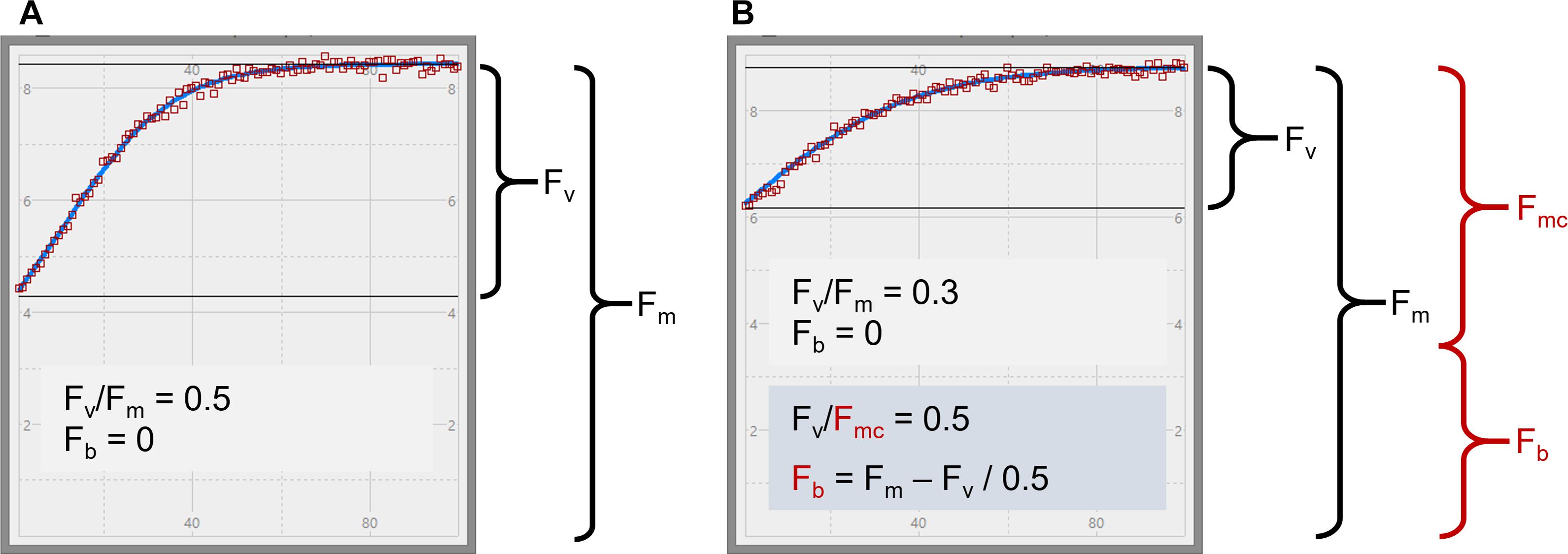
Figure 1. STAF measurements from E. huxleyi illustrating the concept of baseline fluorescence (F_b). In (A) is from a nutrient-replete culture in log-growth phase. In (B) is from a N-limited culture. Two plausible explanations for the lower F_v/F_m in (B) are considered within the main text. The first assumes that F_b is zero, as indicated by the black text in (B), and the second assumes that F_b has a value that accounts for the entire difference in F_v/F_m between (A) and (B), as indicated by the red text. F_mc is the baseline-corrected value of F_m.

In addition to the STAF and flash O₂ measurements used to generate K_a^S values, the same measurement systems were used to run fluorescence light curves (FLCs) and oxygen light curves (OLCs) on all eleven phytoplankton species. The data generated from these measurements allowed for direct comparison of PhytoGO and JV_PII (from Equation 5) at multiple points through the light curves.

This first set of experiments provided evidence for a wider range of K_a values across species and environmental conditions than was evident in the earlier studies of Oxborough et al. (2012) and Silsbe et al. (2015). Although the intra-species variance of K_a values (between values determined for nutrient-replete and N-limited cultures) could confidently be linked to baseline fluorescence, the inter-species variance was more easily explained in terms of the package effect. To test this hypothesis, an additional set of measurements were made on 11 phytoplankton species, of which six were common to the first set of experiments. The species were selected to cover a wide range of cell sizes and optical characteristics. As before, K_a^S values were generated from parallel flash O₂ and STAF measurements. The STAF measurements were made using FastBallast fluorometers (CTG Ltd., as before) fitted with narrow bandpass filters centered at 680 and 730 nm. These wavebands were chosen because chlorophyll a fluorescence is absorbed much more strongly at 680 nm than at 730 nm. It follows that attenuation of fluorescence emission due to the package effect will be much higher at 680 nm than at 730 nm and thus that variability of the package effect among species should correlate with the ratio of fluorescence outputs measured at 730 nm and 680 nm. To allow for comparison with the existing FastOcean sensor, a third FastBallast sensor was fitted with the bandpass filter used within FastOcean.

Materials and Methods

Phytoplankton Cultures (N-Limited Experiments)

Semi-continuous phytoplankton cultures were maintained and adapted to nutrient-replete conditions. All cultures were grown in f/2 medium with silicates omitted where appropriate (Guillard, 1975).

The experimental work covered a period of several months. The initial work was conducted at the University of Essex and incorporated six phytoplankton species (Table 1). Cultures were maintained at 20°C in a growth room (Sanyo Gallenkamp PLC, United Kingdom) and illuminated by horizontal fluorescent tubes (Sylvania Luxline Plus FHQ49/T5/840, United Kingdom). The Light:Dark (L:D) cycle was set at 12 h:12 h. Neutral density filters were used to generate low light and high light conditions (photon irradiances of 30 and 300 μmol photons m^-2 s^-1, respectively). 300 mL culture volumes were maintained within 1 L Duran bottles. Cultures were constantly aerated with ambient air and mixed using magnetic stirrers.

TABLE 1

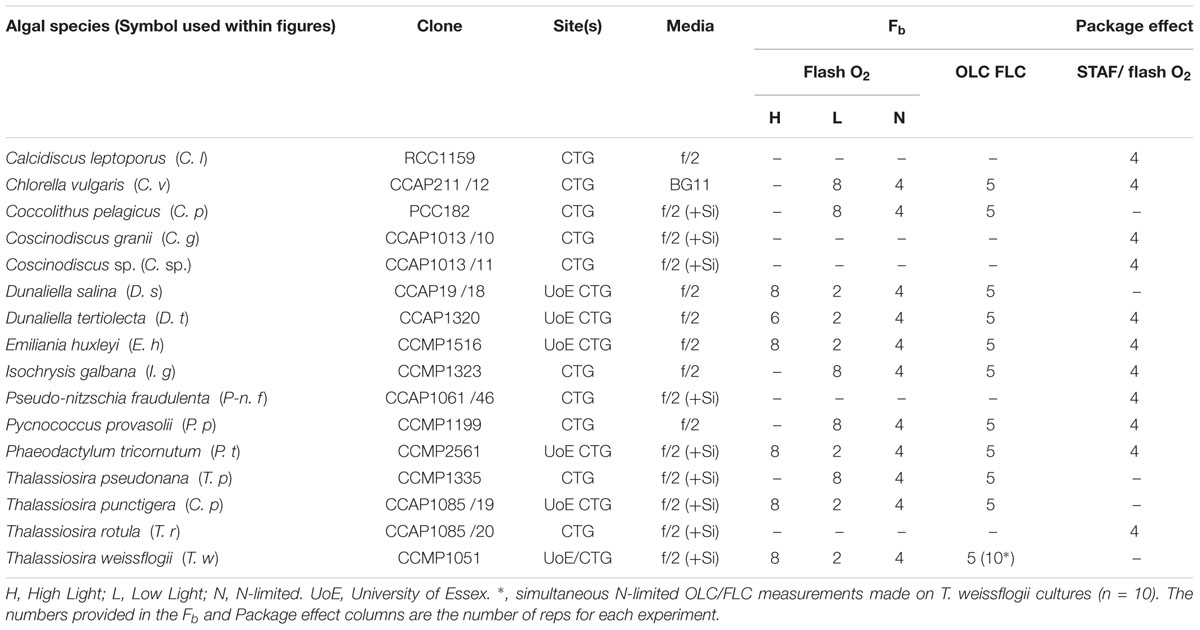
Table 1. List of cultures used within each experiment.

TABLE 2

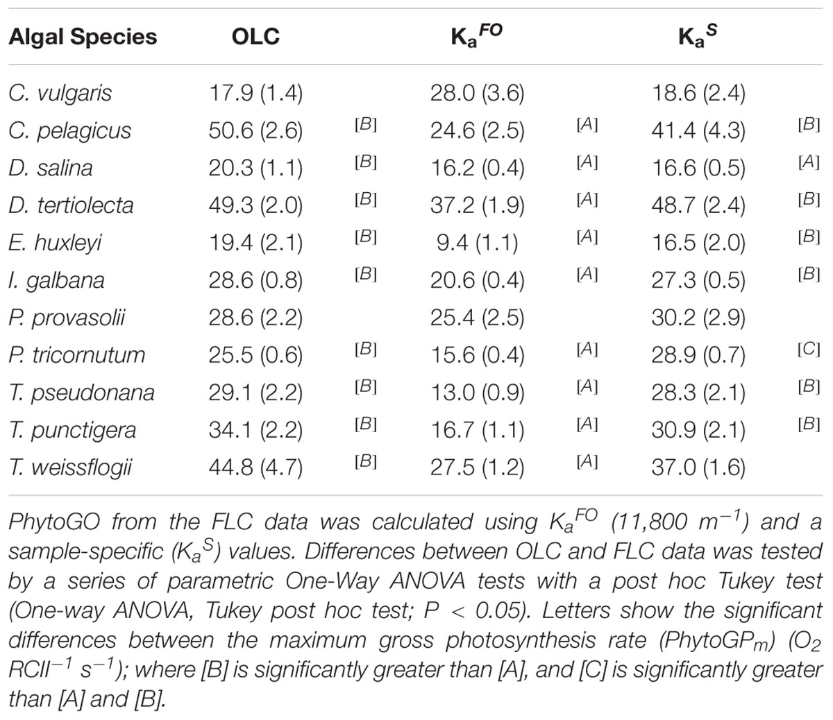
Table 2. The maximum phytoplankton gross photosynthesis rates (PhytoGO_m) from simultaneous OLC and FLC measurements of the 11 nutrient-replete phytoplankton cultures measured in Experiment 1.

Additional experiments, incorporating the remaining five species, were conducted at CTG Ltd. (as before). Cultures were maintained as 30 mL aliquots within filter-capped tissue culture flasks (Fisher Scientific, United Kingdom: 12034917). A growth temperature of 20°C was maintained by placing the flasks within a water bath (Grant SUB Aqua Pro 2 L, United States). Low light illumination (photon irradiance of 30 μmol photons m^-2 s^-1) was provided from white LED arrays (Optoelectronic Manufacturing Corporation Ltd. 1ft T5 Daylight, United Kingdom). The L:D cycle was set at 12 h:12 h.

The N-limited cultures were sub-cultured from the nutrient-replete cultures. High light-grown cultures were used for the six species interrogated at the University of Essex. In all cases, the growth photon irradiance of the original culture was maintained after sub-culturing. All N-limited cultures were grown into the stationary growth phase using N-limiting f/2 medium before experimental measurements were made.

Phytoplankton Cultures (Package Effect Experiments)

All package effect experiments were conducted at CTG Ltd. Cultures were maintained as 30 mL aliquots within filter-capped tissue culture flasks (Fisher Scientific, United Kingdom: 12034917). A growth temperature of 20°C was maintained by placing the flasks within a water bath (Grant SUB Aqua Pro 2 L, United States). Low light illumination (photon irradiance of 30 μmol photons m^-2 s^-1) was provided from white LED arrays (Optoelectronic Manufacturing Corporation Ltd. 1ft T5 Daylight, United Kingdom). The L:D cycle was set at 12 h:12 h.

Setup for OLCs and Flash O₂ Measurements

All OLCs and flash O₂ measurements were made using an Oxygraph Plus system (Hansatech Instruments Ltd, Norfolk, United Kingdom). The sample volume was always 1.5 mL and a sample temperature of 20°C was maintained using a circulating water bath connected to the water jacket of the DW1 electrode chamber. The sample was mixed continuously using a magnetic flea (as supplied with the Oxygraph Plus system). Illumination was provided from an Act2 laboratory system (CTG Ltd, as before). The source comprised three blue Act2 LED units incorporated within an Act2 Oxygraph head. Automated control of continuous illumination during OLCs or the delivery of saturating pulses during flash O₂ measurements was provided by an Act2 controller and the supplied Act2Run software package.

Dilution of Samples Between Flash O₂ and STAF Measurements

The N-limited and dual waveband experiments included determination of K_a^S values. In all cases, the required dark STAF measurements of F_o and σ_PII were made after the flash O₂ measurements. In all cases, filtered medium was used to dilute the sample between Oxygraph and STAF measurements.

Chlorophyll a Extraction

In all cases, the concentrated sample used for flash O₂ or OLCs was normalized to the parallel dilute STAF sample used to generate F_o and σ_PII or FLC data through direct measurement of chlorophyll a concentration from both samples.

Chlorophyll was quantified by pipetting 0.5 mL of each sample into 4.5 mL of 90% acetone and extracting overnight in a freezer at -20°C (Welschmeyer, 1994). Samples were re-suspended and centrifuged at approximately 12,000 × g for 10 min and left in the dark (∼30 min) to equilibrate to ambient temperature. Raw fluorescence from a 2 mL aliquot was measured using a Trilogy laboratory fluorometer (Turner, United Kingdom). The chlorophyll a concentration was then calculated from a standard curve.

Setup for Dark STAF Measurements and FLCs (N-Limited Experiments)

All STAF measurements for the N-limited experiments were made using a FastOcean sensor in combination with an Act2 laboratory add-on (CTG Ltd, as before). The Act2 FLC head was populated with blue LEDs. A water bath was used as a source for the FLC head water jacket, maintaining the sample temperature at 20°C.

Flash O₂ Measurements for Determining Sample-Specific K_a Values

The density of photochemically active PSII complexes within each sample was determined using the flash O₂ method (Mauzerall and Greenbaum, 1989; Suggett et al., 2003; Silsbe et al., 2015). The standard flash used was 120 μs duration on a 24 ms pitch at a photon irradiance of 22,000 μmol photons m^-2 s^-1.

The concentration of photochemically active PSII centers is proportional to the product of gross O₂ evolution rates (E₀) and the reciprocal of flash frequency (Hz). The basic theoretical assumptions are that all photochemically active PSII centers undergo stable charge separation once during each flash, that all photochemically active PSII centers re-open before the next flash and that four stable charge separation events are required for each O₂ released. In reality, small errors are introduced because some centers do not undergo stable charge separation with each flash (misses) while some centers will undergo more than one stable charge separation event with each flash (multiple hits).

The following checks were applied with all samples:

• The proportion of PSII centers closed during each flash was verified by comparison with sequences of 120 μs flashes on a 24 ms pitch at a photon irradiance of 13,800 μmol photons m^-2 s^-1

• The default flash pitch of 24 ms was compared against 16 and 36 ms to assess the accumulation of closed PSII centers, with 120 μs flashes of 22,000 μmol photons m^-2 s^-1 being applied in all three cases

• Sequences of 180 and 240 μs flashes on a 24 ms pitch at a photon irradiance of 22,000 μmol photons m^-2 s^-1 were applied to assess multiple hits

In all cases, a flash duration of 120 μs duration at a photon irradiance of 22,000 μmol photons m^-2 s^-1 on a 24 ms pitch provided more than 96% saturation, with no evidence of a significant level of multiple hits or the accumulation of closed PSII centers.

Parallel OLC and FLC Measurements (N-Limited Experiments)

A series of parallel replicate OLC/FLC measurements were made on all nutrient-replete cultures, as well as for the N-limited Thalassiosira weissflogii culture (Table 1). The 10–12 light steps were identical between the parallel OLC and FLC measurements. The sequences always started with a dark step, with all subsequent steps lasting 180 s. Additional dark steps were incorporated after every third light step. The dark respiration rate (R_d) was assessed before, during and after the OLC. The R_d values measured during and after the OLC were always within 8% of the initial R_d (n = 65). The FastOcean ST sequence comprised 100 flashlets on a 2 μs pitch. Each acquisition was an average of 16 sequences on a 100 ms pitch. The auto-LED and auto-PMT functions incorporated within the Act2Run software were always active.

The reported gross O₂ evolution rates (E₀) were taken as the sum of measured net O₂ evolution (P_n) and R_d (Equation 9).

$$\begin{array}{c}{\text{E}}_{\text{0}}\text{=}{\text{P}}_{\text{n}}\text{+}{\text{R}}_{\text{d}}\left(9\right)\end{array}$$

OLC and FLC Curve Fits (N-Limited Experiments)

OLCs and FLCs are variants of the widely used P-E (photosynthesis – photon irradiance) curve. For OLCs, the metric for photosynthesis is the rate at which O₂ is evolved through water oxidation by PSII. For FLCs, the metric for photosynthesis is the relative rate of PSII photochemistry, which is assessed as the product of ϕ_PII and E. In the absence of baseline fluorescence (when F_b = 0), the parameter F_q’/F_m’ can be used to provide an estimate of ϕ_PII. It follows that FLC curves can be generated by plotting E against the product of baseline corrected F_q′/F_m′ (F_q′/F_mc′) and E.

There are three basic parameters derived from all P-E curve fits: α, E_k, and P_m. The value of α provides the initial slope of the relationship between E and P. E_k is an inflection point along the P-E curve which is often described as the light saturation parameter (Platt and Gallegos, 1980). P_m is the maximum rate of photosynthesis.

The FLC curve fits within this study were generated by the Act2Run software (CTG Ltd, as before). The curve fitting routine within Act2Run is a two-step process which takes advantage of the fact that the signal to noise within FLC data is highest during the initial part of the FLC curve. In the first step (the Alpha phase), Equation 10 is used to generate values for α and E_k (Webb et al., 1974; Silsbe and Kromkamp, 2012). The overall fit is an iterative process that minimizes the sum of squares of the difference between observed and fit values. During the Alpha fit, a significant weighting on the initial points (low actinic E values) is generated by multiplying each square of the difference by (F_q′/F_mc′)². This approach normally generates a good fit up to E_k, but overshoots beyond this point. Consequently, the P_m values generated by the Alpha phase are generally too high.

$$\begin{array}{c}\frac{{\text{F}}_{\text{q′}}}{{\text{F}}_{\text{m′}}}=\text{ α}·{\text{E}}_{\text{k}}·(1-{\text{e}}^{-{\text{E/E}}_{\text{k}}})·{\text{E}}^{-1}\left(10\right)\end{array}$$

In the second step (the Beta phase) Equation 11 is used to improve the value of P_m. This step includes a second exponential which is only applied to data points at E values above the E_k value generated by the Alpha phase. The sum of squares of the difference between observed and fit values is not weighted during the Beta phase. This approach forces ϕ_PII at E_k to be 63.2% of α.

$$\begin{array}{c}\frac{{\text{F}}_{\text{q′}}}{{\text{F}}_{\text{m′}}}=(\alpha ·{\text{E}}_{\text{k}}·[1-{\text{e}}^{-{\text{E/E}}_{\text{k}}}]-\text{ β}·{\text{E}}_{k\text{β}}·[1-e^{-\{\text{E}-{\text{E}}_{\text{k}}\}/E_{k\text{β}}}])·{\text{E}}^{-1}\left(11\right)\end{array}$$

The signal to noise for OLC data tends to increase with E (the opposite of what happens with FLC data). Consequently, the fitting method used for the FLC data is not appropriate for OLC data as it is highly dependent on having a good signal to noise during the early part of the curve. The iterative OLC data fits used Equations 12 and 13 (Platt and Gallegos, 1980).

$$\begin{array}{c}\text{P}\text{=}{\text{P}}_{\text{S}}·(1-{\text{e}}^{(-\text{ α}·{\text{E/P}}_S)})·({\text{e}}^{(-\text{ β}·{\text{E/P}}_{\text{S}})})\left(12\right)\end{array}$$

$$\begin{array}{c}{\text{P}}_{\text{m}}\text{=}{\text{P}}_{\text{S}}·\left(\frac{\text{α}}{\text{α}+\text{β}}\right)·{\left(\frac{\text{β}}{\text{α}+\text{β}}\right)}^{\frac{\text{β}}{\text{α}}}\left(13\right)\end{array}$$

Within these equations, P_s and β improve some fits by incorporating a phase that accounts for possible photoinactivation of PSII complexes and/or supra-optimal levels of PSII downregulation (photoinhibition).

Direct comparison of α and β between the FLC and OLC is problematic because while α is incorporated through the entire curve for both fits, β is only incorporated beyond E_k for the FLC and through the entire curve for the OLC. For this reason, direct comparison between FLC and OLC data was focused on P_m values.

Setup for the Package Effect STAF Measurements

STAF measurements were made using three FastBallast sensors (CTG Ltd, as before). Each sensor was fitted with one of the following bandpass filters:

730 nm bandpass, 10 nm FWHM (Edmund Optics, United Kingdom; part number 65-176)

680 nm bandpass, 10 nm FWHM (Edmund Optics, United Kingdom; part number 88-571)

682 nm bandpass, 30 nm FWHM (HORIBA Scientific, United Kingdom; part number 682AF30)

Where FWHM is Full Width at Half Maximum. These filters are, hereafter, termed B730, B680 and B682, respectively. B682 is the standard bandpass filter fitted within FastOcean and FastBallast fluorometers and was included here for comparison.

The emission peak for PSII fluorescence is centered at 683 nm and is Stokes shifted from a strong absorption peak centered at 680 nm. Consequently, reabsorption of PSII fluorescence defined by B680 is close to maximal and is also very high when PSII fluorescence is defined by B682. In contrast, reabsorption of PSII fluorescence within the waveband defined by B730 is minimal.

Because the FastBallast sensor does not incorporate a water jacket, all measurements were made in a temperature-controlled room at 20°C. The FastBallast units were always switched on immediately before each test and automatically powered down once a test had finished. This procedure prevented any measurable increase in temperature within the FastBallast sample chamber during testing.

Calibration of FastBallast units does not include an absolute assessment of the measurement LED photon flux density (which is included within the calibration of FastOcean sensors). Consequently, there is no instrument-type specific K_a available for FastBallast. To get around this limitation, the LED output was maintained at a constant level for all measurements. This allowed Equation 14 to be used in place of Equation 4.

$$\begin{array}{c}{\text{K}}_{\text{R}}=[\text{PSII}]·\frac{{\text{J}}_{\text{PII}}}{{\text{F}}_{\text{o}}}\left(14\right)\end{array}$$

Where K_R is the instrument-specific constant defined by Oxborough et al. (2012) with units of photons m^-3 s^-1 and JPII is the initial rate of PSII photochemical flux during a STAF pulse, with units of electrons PSII^-1 s^-1. As before, it is assumed that each photon used to drive PSII photochemistry results in the transfer of one electron.

Samples used for the FastBallast STAF measurements were prepared by diluting a small aliquot from the sample used for the associated flash O₂ measurement. Sixty mL of cell suspension was prepared and divided equally among the three FastBallast sample chambers. Samples were dark-adapted for at least 5 min before measurements were made.

Each sample was run through the three FastBallast units simultaneously using the FaBtest software supplied with the FastBallast fluorometer (CTG Ltd, as before). This test involved continuous application of 400 μs saturating pulses at 10 Hz to a slowly stirred 20 mL sample for 8 min. Only 0.5 mL of the sample is illuminated by the saturating pulse at any point in time. Stirring the sample ensured that the entire sample was interrogated during the test and prevented the accumulation of closed PSII reaction centers. The mean value of F_v was extracted from each test result.

Following the initial measurement, a spike of Basic Blue 3 (BB3) was added to each sample to increase the extracellular baseline fluorescence. BB3 is a water-soluble fluorescent dye, which absorbs throughout the visible range and has a broad emission spectrum centered at approximately 690 nm (Sigma-Aldrich, Saint Louis, MA, United States). As such, it can be used to simulate non-variable fluorescence emission from any source, including CDOM and free chlorophyll a. The BB3 was dissolved in MilliQ water to a final concentration of 118 μM. The volume of the BB3 spike was never more than 30 μL within each 20 mL sample. After spiking with BB3, each sample was dark-adapted for 5 min followed by a second test. In all cases, the F_b generated by addition of BB3 was at least three times the value of the original F_v and, consequently, decreased F_v/F_m by approximately 65%.

Terminology

A structured approach has been taken in derivation of the parameters used within this manuscript. As baseline fluorescence is central to this study, new fluorescence terms to describe baseline-corrected values of existing fluorescence terms have been introduced. Otherwise, the parameters are structured around root terms that are widely used within the fluorescence community.

Table 3 provides terms used to describe the fluorescence signal at any point. Table 4 provides commonly used parameters derived from the terms in Table 3. Tables 5–7 show the derivation of terms used for the yields, rate constants, absorption cross sections and absorption coefficients applied to PSII energy conversion processes.

TABLE 3

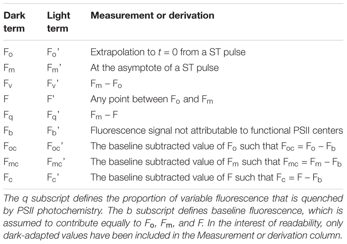
Table 3. The o, m, and v subscripts define the origin (of variable fluorescence), maximum fluorescence and variable fluorescence, respectively.

TABLE 4

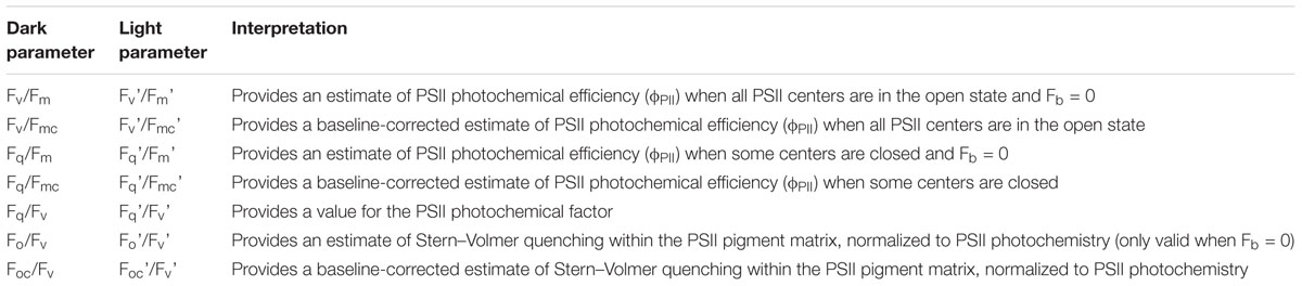
Table 4. Fluorescence parameters derived using the terms within Table 3.

TABLE 5

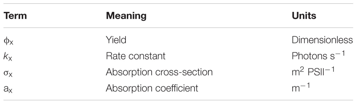
Table 5. Root terms used in the derivation of parameter ‘x’ within Table 7.

TABLE 6

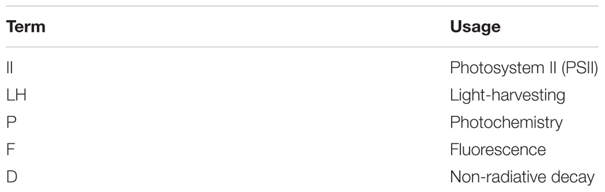
Table 6. Subscripts used for derivation of parameters within Table 7.

TABLE 7

Table 7. Parameters derived from the root terms and subscripts within Tables 5, 6, respectively.

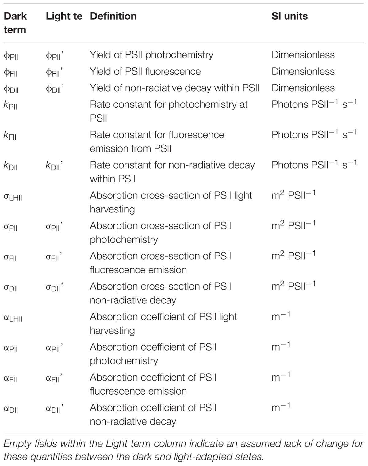
The root terms and subscripts provided in Tables 5, 6, respectively, are very widely used (examples include Butler and Kitajima, 1975; Kolber et al., 1998; Baker and Oxborough, 2004; Oxborough et al., 2012). These tables were constructed to introduce consistency and minimize ambiguity: particularly with the distinction between absorption cross-sections and absorption coefficients. It should also be noted that the ‘optical absorption cross-section of PSII’ and ‘effective absorption cross-section of PSII’ (both unit area per photon) employed by Kolber et al. (1998) are, in terms of usage, equivalent to the absorption cross-sections of PSII light-harvesting and PSII photochemistry (both unit area per PSII), respectively.

Results

Sample-Specific K_a Values Under Nutrient-Replete and N-Limited Conditions

The sample-specific values of K_a (K_a^S) for all nutrient-replete, low light grown cultures ranged from 7,822 m^-1 for C. vulgaris to 25,743 m^-1 for T. pseudonana (Figure 2A). Of the six species grown under both low and high light, only D. salina exhibited a significant difference in the K_a^S values between light treatments (Supplementary Table 1). In all cases, the N-limited K_a^S values were significantly lower than for the nutrient-replete samples from which they were sub-cultured (Figure 2A). These lower K_a^S values were matched to lower values of F_v/F_m (Supplementary Table 1).

FIGURE 2

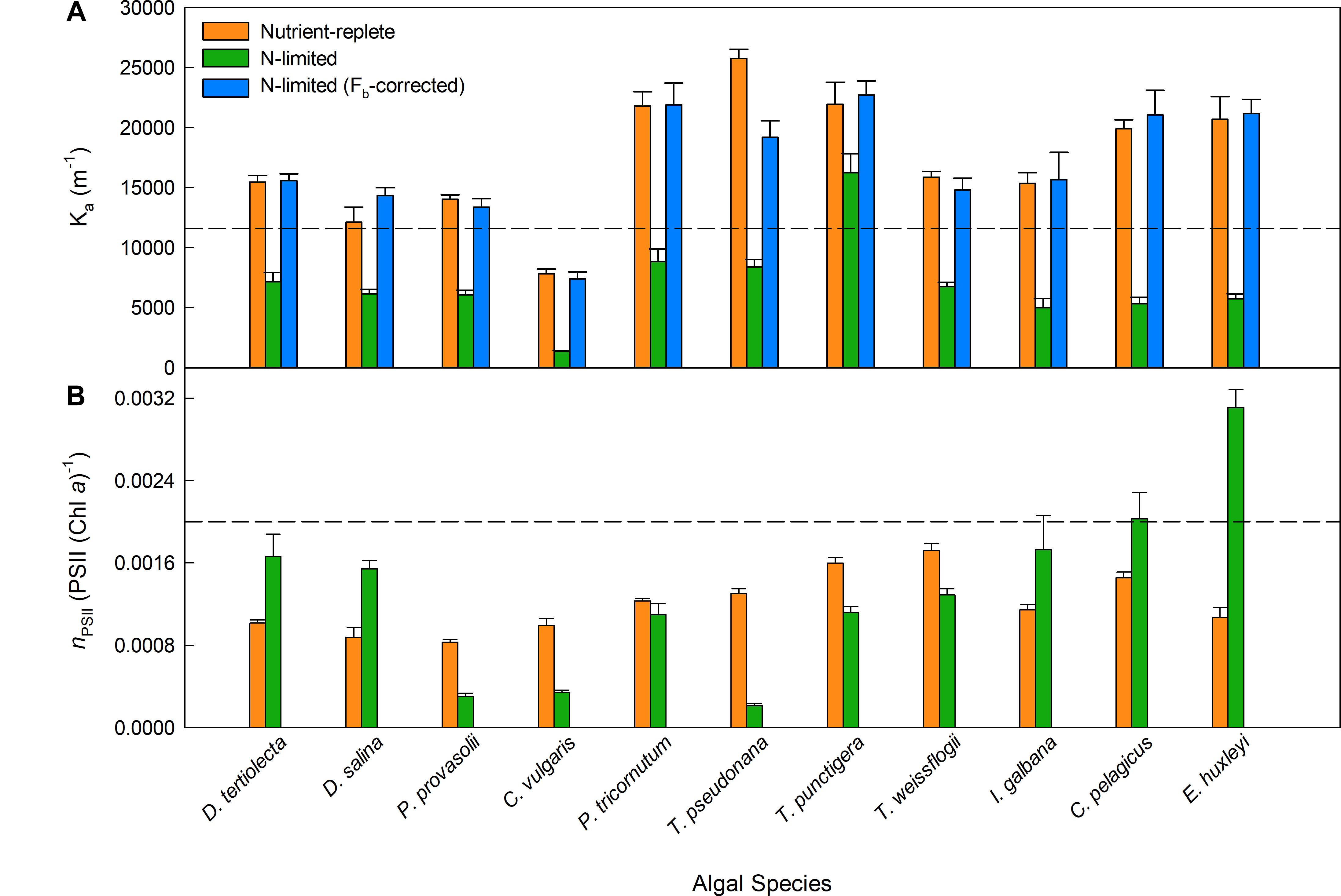
Figure 2. Variability in K_a (A) and n_PSII (B) values measured across a range of phytoplankton species. In (A), the consensus F_v/F_mc value of 0.518 (see main text) was used to calculated F_b for each culture when the measured F_v/F_m was lower than 0.518. F_b was subtracted from the measured F_o and F_m. The dashed line represents K_a^FO (11,800 m^-1). Significant differences were tested by a series of parametric t-tests (t-test; P < 0.05); however, if normality was not achieved after data transformation a Mann–Whitney Rank Sum test was performed. All nutrient-replete and uncorrected N-limited K_a values were significantly different. In (B), the number of PSII reaction centers per chlorophyll a molecule was calculated from flash O₂ measurements and chlorophyll a extractions. More details are provided within Section “Materials and Methods.”

As discussed in the introduction, there are two mechanisms that could cause sub-maximal F_v/F_m values: dark-persistent Stern–Volmer quenching and baseline fluorescence. Importantly, the absorption method is insensitive to Stern–Volmer quenching while baseline fluorescence can introduce a significant error in the calculation of JV_PII. In the context of these tests, the lower values of both sample-specific K_a and F_v/F_m values observed within the N-limited cultures, when compared to the nutrient-replete values, are entirely consistent with a baseline fluorescence-induced error being introduced by, for example, the accumulation of photoinactivated PSII complexes and/or other energetically uncoupled complexes. To test this possibility, Equation 15 (Oxborough, 2012) was used to derive a theoretical F_v/F_mc value that could be applied across all N-limited cultures.

$$\begin{array}{c}{\text{F}}_{\text{b}}\text{=}{\text{F}}_{\text{m}}-\frac{{\text{F}}_{\text{v}}}{({\text{F}}_{\text{v}}{\text{/F}}_{\text{mc}})}\left(15\right)\end{array}$$

Where F_mc is the F_b-corrected value of the measured F_m (see Terminology). When using this equation, F_m and F_v are measured from the sample and F_v/F_mc is an assumed baseline corrected value of F_v/F_m for the photochemically active PSII complexes within the sample (see Figure 1). The single, consensus value of F_v/F_mc used was generated iteratively, by minimizing the total sum of squares for the differences in K_a^S values from nutrient-replete cultures and corrected N-limited cultures.

Applying an F_b-correction within Equation 15 brings the N-limited K_a^S values for all but one species (T. pseudonana) up to the point where they are not significantly different from the matched nutrient-replete culture values and resulted in a consensus F_v/F_mc value of 0.518. Even with T. pseudonana, the F_b-corrected value is much closer to the nutrient-replete value than is the uncorrected N-limited value. The observation that the consensus F_v/F_mc value required for the F_b-corrected values is slightly lower than most of the F_v/F_m values measured from the nutrient-replete cultures (see Supplementary Table 1) may indicate that the photochemically active PSII complexes within the N-limited cultures are operating at a slightly lower efficiency that the photochemically active PSII complexes within the nutrient-replete cultures.

The dashed line within Figure 2A shows the default K_a value of 11,800 m^-1 that is currently provided for the FastOcean sensor (hereafter, K_a^FO). Although this value falls within the mid-range of K_a^S values for the nutrient-replete cultures, there is considerable variability around this default value; for example, K_a^FO is approximately 50% higher than the nutrient-replete K_a^S value for C. vulgaris and less than 50% of the equivalent value for T. pseudonana.

Interspecific Variability in K_a and Chl PSII^-1

A comparison between n_PSII and K_a is valid because they have a similar proportional impact in the calculation of [PSII] within Equations 2 and 4, respectively. Figure 2B shows n_PSII values for nutrient-replete cultures and N-limited cultures. The dashed line is at a widely used default value for n_PSII of 0.002 Chl PSII-1 (Kolber and Falkowski, 1993; Suggett et al., 2001). There are two noteworthy features within this dataset. Firstly, the range of n_PSII values is very wide, at around 15:1: from less than 0.0002 Chl PSII^-1 for the N-limited T. pseudonana to more than 0.003 Chl PSII^-1 for N-limited E. huxleyi. Secondly, there is a lack of consistency between n_PSII values from nutrient-replete cultures and N-limited cultures: five species show higher n_PSII values for the N-limited cultures while the remaining six species show lower n_PSII values for the N-limited cultures. Overall, these data provide a good illustration of how an assumed value for n_PSII can introduce large errors in the calculation of JV_PII, which can only be corrected through independent determination of PSII concentration.

Comparison of OLC and FOC Curves

Figure 3 shows OLC and FLC data from all eleven phytoplankton species used within this study. All data are from the nutrient-replete, low light-grown cultures. The FLC values of PhytoGO (y-axes) assume four electrons per O₂ released. Values from the STAF data were derived using either K_a^FO or the K_a^S values shown in Figure 2A. Clearly, in most cases, the match between OLC and FLC is greatly improved by using the K_a^S values in place of K_a^FO. The one exception is Figure 3B (D. salina) where the K_a^S value happens to be very close to K_a^FO.

FIGURE 3

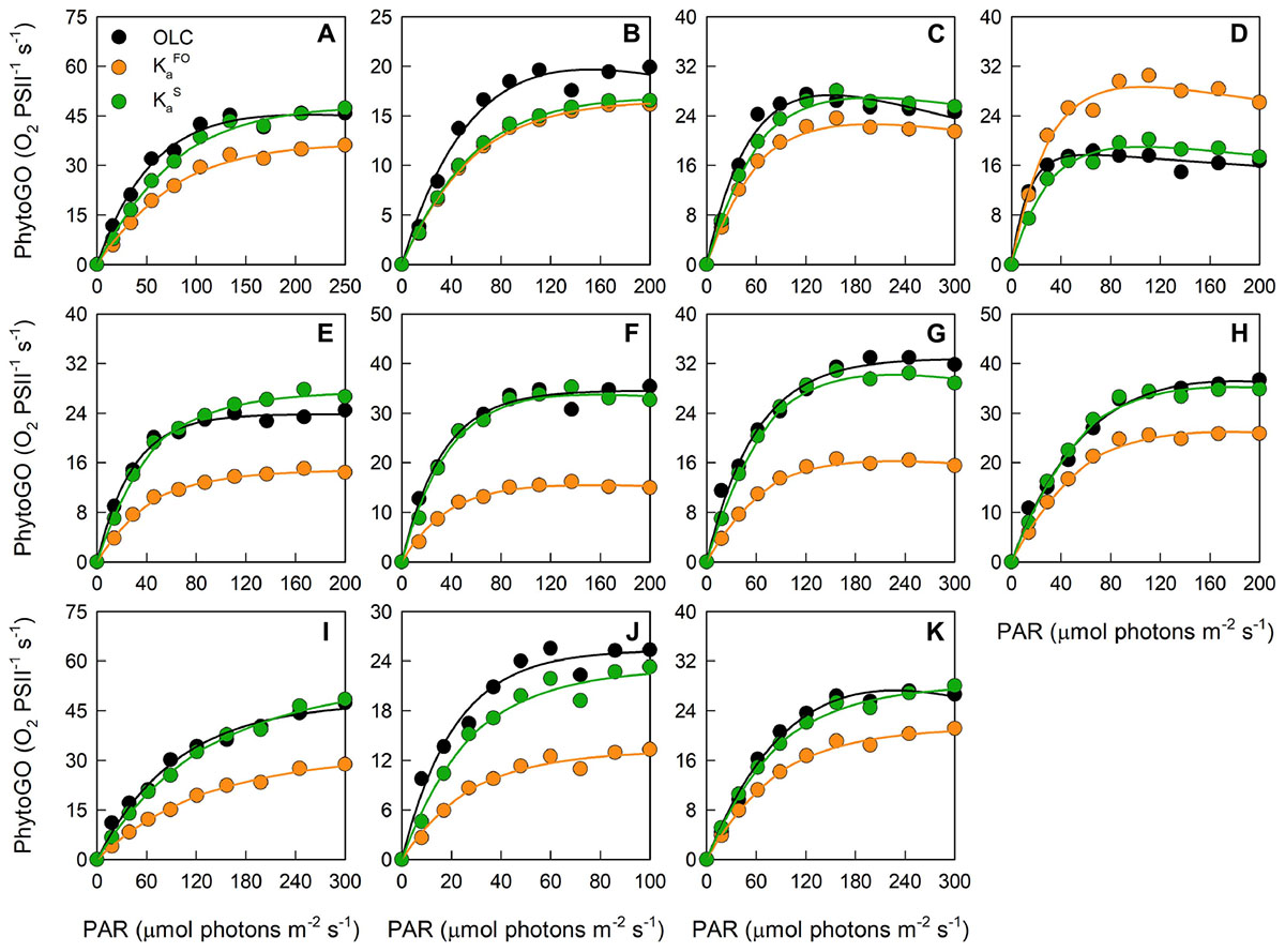
Figure 3. A representative example of simultaneous oxygen light curve (OLC) and fluorescence light curve (FLC) measurements made across all phytoplankton species. The OLC and FLC measurements were made on cultures acclimated to ambient temperature (∼20°C) and low-light (LL = 30 μmol photons m^-2 s^-1). FLC data were standardized to equivalent units of O₂, with both OLC and FLC data normalized to a derived concentration of functional PSII complexes (O₂ PSII^-1 s^-1). FLC data were derived using K_a^FO (11,800 m^-1) or a sample-specific (K_a^S) value. The solid lines represent the P-E curve fits (color-coded to match the data points). (A) = D. tertiolecta; (B) = D. salina; (C) = P. provasolii; (D) = C. vulgaris; (E) = P. tricornutum; (F) = T. pseudonana; (G) = T. punctigera; (H) = T. weissflogii; (I) = C. pelagicus; (J) = E. huxleyi; (K) = I. galbana. PhytoGOm values from all OLC and FLC data fits are shown in Table 2. Replicates from each species (n = 5) are presented in Supplementary Figures 3–12.

The data presented within Figure 4 have been extracted from the OLCs and FLCs within Figure 3 to allow bulk comparison of the measured OLC and FLC PhytoGO values (A and C). Also shown is a comparison of the P_m values (B and D) from the OLC and FLC curve fits. Values were generated using either K_a^FO (A and C) or K_a^S values (B and D).

FIGURE 4

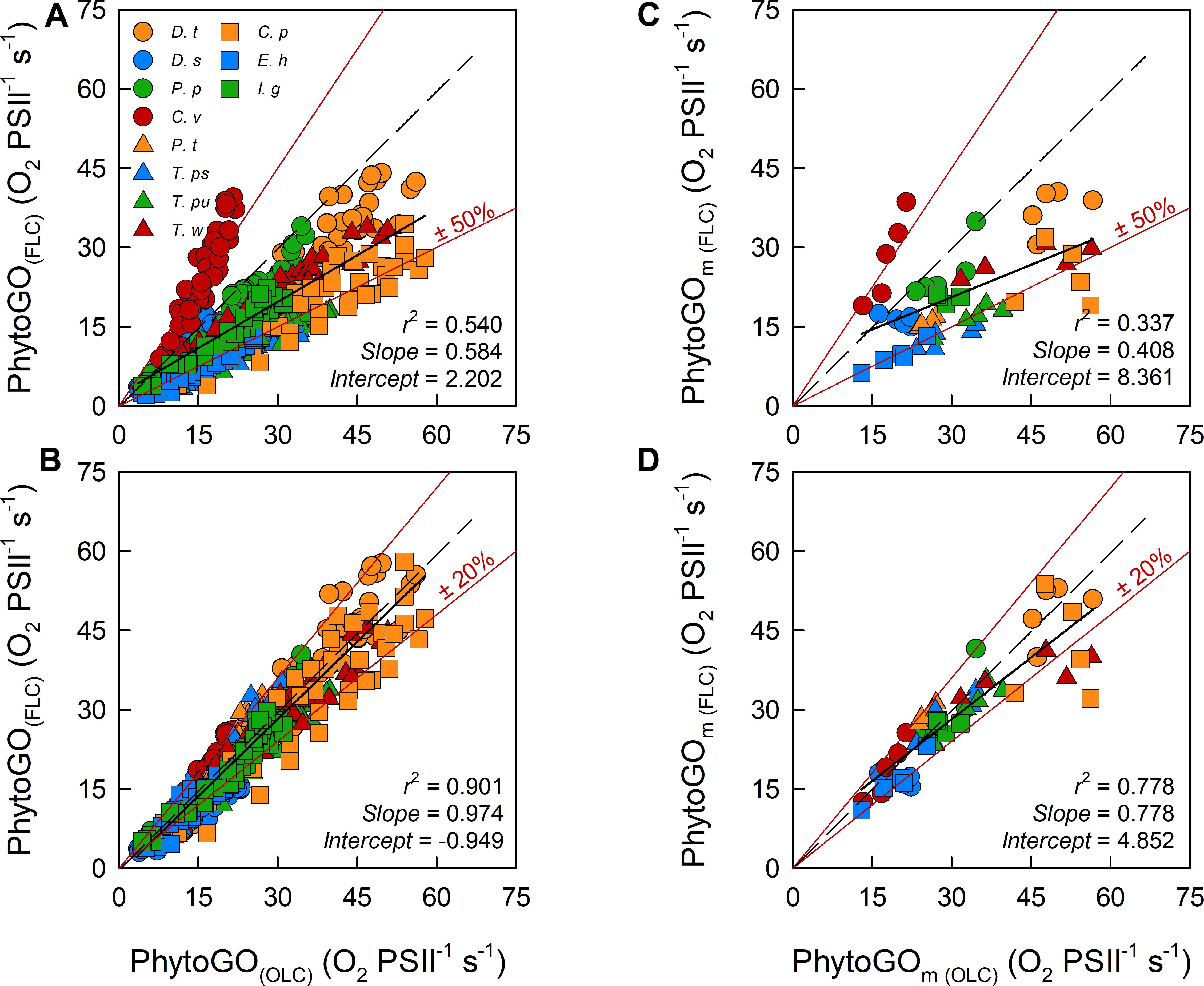
Figure 4. The relationship between the entire photosynthesis-photon irradiance (P-E) curve of PhytoGO (A,C), and the maximum PhytoGO (PhytoGO_m) from simultaneous OLC and FLC measurements (B,D). FLC data were standardized to equivalent units of O₂, with both OLC and FLC data normalized to a derived concentration of functional PSII complexes (O₂ PSII^-1 s^-1). Within (A,B), FLC data were derived using K_a^FO (11,800 m^-1). Within (C,D), K_a^S values were used (see Materials and Methods). Each species consisted of 5 biological replicates. The dashed line represents a 1:1 line, while the solid line is the linear regression used to generate r², slope and intercept values. A key for the symbols in (A) is incorporated within Table 1.

Inevitably, the match between OLC and FLC data, both as the entire PE curve [ANCOVA, F(2, 492) = 1.962, P < 0.001] and P_m values [ANCOVA, F(2, 106) = 1.983, P < 0.001], is improved significantly when K_a^S values (C and D) are used in preference to K_a^FO (A and B). The slope for the K_a^S data is very close to the ’ideal’ of 1.0 and a high proportion of data points fall within the ±20% lines included within the plot [Paired t-test, t(492) = 1.781, P < 0.005]. In contrast, the K_a^FO data have a much lower slope of 0.6 and ±50% lines are required to constrain a similar proportion of points [Paired t-test, t(492) = 17.119, P > 0.005]. The K_a^S values also generate a much better correlation between the values of P_m derived from OLC and FLC curve fits than K_a^FO (D and B, respectively). The slope for the K_a^S data (D), at 0.778, is significantly lower than the ideal of 1.0 [Paired t-test, t(53) = 3.888, P > 0.005]. This lower slope may be at least partly due to differences in the curve fits applied to OLC and FLC data (see Materials and Methods).

The Stability of F_b Under Actinic Light

Clearly, the consensus F_v/F_mc (0.518) in Equation 15 generated a good match between K_a^S values for all but one of the nutrient-replete and N-limited cultures in Figure 2A. In a wider context, it could prove valid to use the consensus F_v/F_mc of 0.518 within Equation 15 when the measured F_v/F_m is lower than this value and assume that F_b is zero when the measured F_v/F_m is above 0.518.

In situations where F_b is non-zero, the calculated value of a_LHII used within Equation 5 is decreased while value of F_q’/F_m’ used within the same equation is increased. The adjustment to a_LHII can largely be justified by the fact that matched F_b and a_LHII values are derived from the same dark-adapted STAF measurement. In contrast, the adjustment to F_q’/F_m’ is potentially more complex, simply because light-dependent NPQ can significantly decrease the maximum fluorescence level between the dark-adapted F_m and light-adapted F_m’ (see Introduction). Given that a proportion of F_b could be from photoinactivated PSII complexes within the same membranes as the photochemically active PSII complexes, it seems reasonable to consider the possibility that NPQ could also quench F_b.

To test the potential for a NPQ-dependent decrease in F_b, additional FLCs were run on the N-limited cultures of T. weissflogii that had been sub-cultured from the low light-grown, nutrient-replete cultures. The value of F_b for the original, nutrient-replete cultures was always assumed to be zero, simply because the measured F_v/F_m from these cultures was always above 0.518. Conversely, the F_v/F_m values measured from the N-limited cultures were always well below the consensus value, at 0.116 ± 0.006.

Figure 5A shows the maximum PhytoGO values (PhytoGO_m), measured as O₂-evolution (x-axis) or calculated using the K_a^S value from the nutrient-replete T. weissflogii of 15,868 m^-1. For these values, F_b was set to zero for both the nutrient-replete cultures and the N-limited cultures. Clearly, while there is good agreement between the measured and calculated values of PhytoGO_m from the nutrient-replete cultures, most of the calculated PhytoGO_m values from the N-limited cultures are much higher than the measured values. As noted previously, failure to correct for F_b results in an overestimate of a_LHII and underestimate of F_q’/F_m’. In this case, it seems reasonable to conclude that the overestimate of a_LHII was greater than the underestimate of F_q’/F_m’, resulting in an overestimate of PhytoGO_m.

FIGURE 5

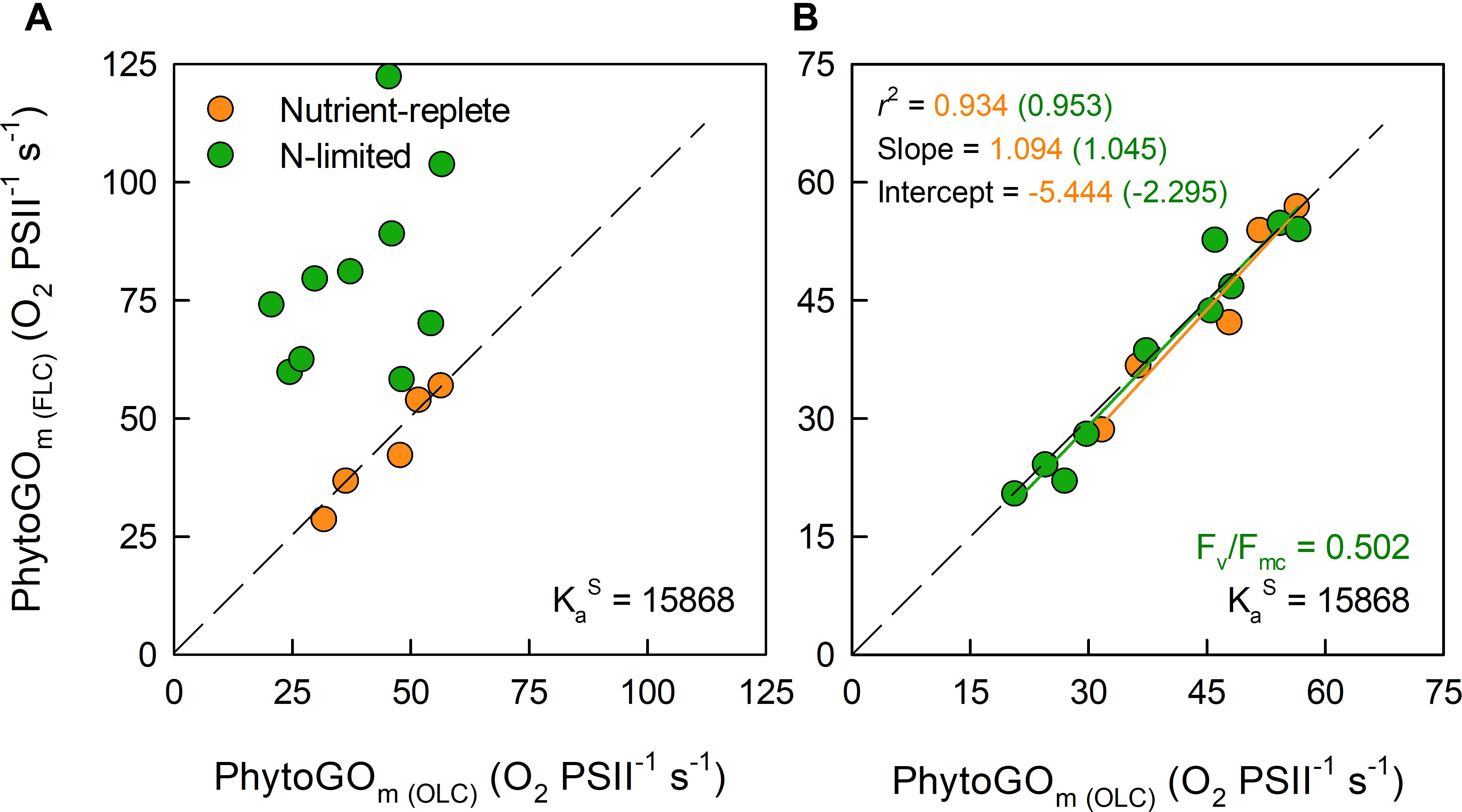
Figure 5. The relationship between simultaneous OLC and FLC measurements of maximum PhytoGO (PhytoGO_m) within N-limited (n = 10) and nutrient replete (n = 5) T. weissflogii cultures. The K_a^S value from the nutrient-replete cultures was applied throughout. In (A), no F_b correction was applied. In (B), the N-limited values were F_b-corrected by applying a consensus F_v/F_mc value of 0.502. Further details are provided within Section “Materials and Methods.”

For Figure 5B, Equation 15 was used to generate a consensus F_v/F_mc specific to the N-limited cultures. This consensus value was reached by minimizing the sum-of-squares for the regression line through the N-limited data by allowing F_b to vary. The mean consensus F_v/F_mc from this fit (0.502) is within 3% of the consensus value derived from the dark-adapted data presented in Figure 2. In contrast, the average NPQ-dependent decrease from dark-adapted F_m to the light-adapted F_m’ measured at P_m was always more than 30% (data not shown). Consequently, these data do not imply significant quenching of F_b between the dark-adapted state and P_m.

Dual Waveband STAF Measurements to Correct for the Package Effect

We hypothesized that variability in the package effect could account for the variance of K_a^S values within Figure 2A. As previously noted within Materials and methods, three FastBallast units were used to measure fluorescence centered at 730 and 680 nm (designated B730 and B680, both with 10 nm FWHM) and 682 nm (designated B682 with 30 nm FWHM), respectively.

We generated ratios of the F_v measured using the bandpass filter centered at 730 nm to F_v measured using the bandpass filters centered at 680 nm (F_v^730/680) or 683 nm (F_v^730/683). Within Figure 6, the values of these ratios are plotted against sample-specific values of K_R (Figures 6A,D, respectively). The linear regressions generated from the data in Figures 6A,D were used to generate F_v-derived values of K_R which are shown in Figures 6B,E, respectively.

FIGURE 6

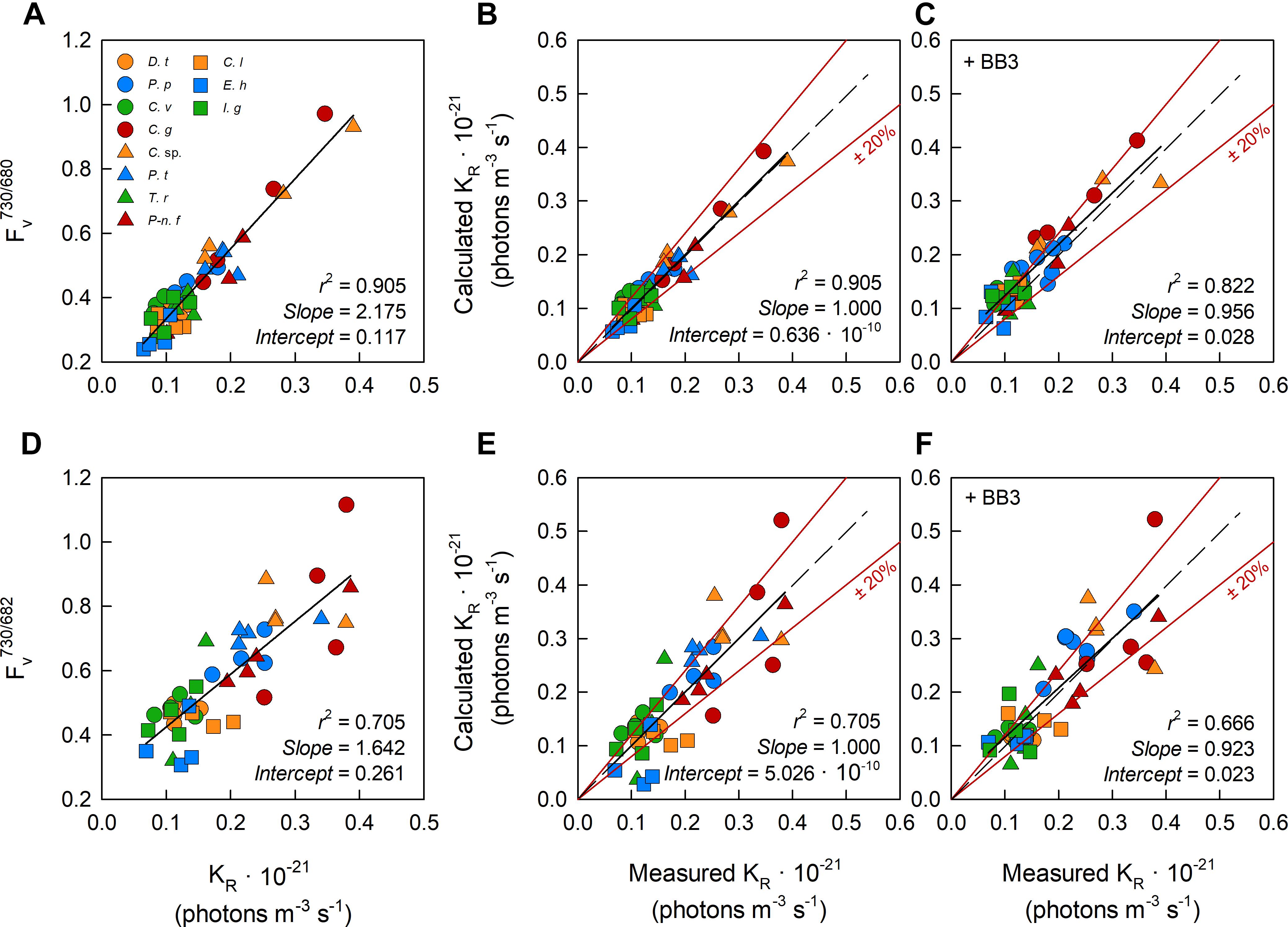
Figure 6. The relationship between dual wavelength STAF measurements and K_R values generated using the flash O₂ method. The leftmost panels show the ratio of F_R measured by B730 to F_v measured by B680 (A) and F_v measured by B730 to F_v measured by B682 (D) against the measured K_R value from parallel measurements of flash O₂. The middle panels (B,E) show the relationship between flash O₂-derived K_R and dual waveband-derived K_R values. The dual waveband K_R values within these panels were derived using the slopes and offsets reported in (A,D), as appropriate. The rightmost panels (C,F), show the same relationships as reported in (B,E), respectively, but in the presence of extracellular baseline fluorescence (F_b) generated by a spike of BB3 (see Materials and Methods). The dashed lines in each panel represents a 1:1 slope, the solid black line is the linear regression. The solid red lines represent ± 20% of the regression values.

$$\begin{array}{c}\text{Calculated}{\text{K}}_{\text{R}}=\frac{{\text{F}}_{\text{v}}^{730/680}-Intercept}{Slope}\left(16\right)\end{array}$$

Equation 16 provides the conversion between A and D. For the equivalent conversion between B and E, F_v^730/680 was replaced with F_v^730/683. Slope and Intercept are the regression line values from A or D, as appropriate. The calculated K_R values within C and F were generated by combining the observations of F_v^730/680 and F_v^730/683 from samples with the added BB3 with the Slope and Intercept from A and D, as appropriate.

One feature that is immediately clear from these data is the much tighter grouping of points along the regression lines for the F_v^730/680 data (Figures 6A–C) than the F_v^730/683 data (Figures 6D–F). This indicates that the 30 nm FWHM of the 682 nm bandpass filter is too broad to adequately isolate the fluorescence generated close the 680 nm absorption peak and, consequently, that the 10 nm FWHM 680 nm bandpass filter is the better choice for these measurements.

All 11 species used within the package effect tests were grown under nutrient-replete conditions and exhibited F_v/F_m values that were above the consensus value of 0.518 generated from the first part of this study. BB3 was added to each sample within the package effect tests to simulate the lower F_v/F_m values that are frequently observed under conditions of stress. The expectation was that fluorescence from the added BB3 would increase F_b but have minimal impact F_v and, as a consequence, that the slope of the relationship between calculated and measured K_R values would not be significantly affected by a BB3-dependent increase in F_b. The absence of significant changes in slope between Figures 6B,C and between Figures 6E,F are consistent with this expectation.

Discussion

Determination of JV_PII using the absorption method described by Oxborough et al. (2012) provides a method for estimating PhytoGO and PhytoPP on much wider spatiotemporal scales than can be achieved by conventional measurements of O₂ evolution or ¹⁴C fixation, respectively. This study was undertaken to assess the extent to which baseline fluorescence and the package effect could introduce errors into the calculation of JV_PII (Equation 5).

With regard to baseline fluorescence (F_b), the underlying question was whether sub-maximal dark-adapted value of F_v/F_m could be attributed to F_b or downregulation of PSII photochemistry by dark-persistent Stern–Volmer quenching or some combination of the two. The data presented within Figure 2A provides strong evidence that, for the examples presented within this study, F_b is by far the dominant contributor to sub-maximal F_v/F_m values. Although this interpretation may not hold for all phytoplankton species and environmental conditions, this study provides a straightforward, practical approach to addressing the question of how universally valid an F_b correction to low sub-maximal dark-adapted F_v/F_m values might be.

We conclude that no correction for baseline fluorescence should be applied when the dark-adapted F_v/F_m is above a certain consensus value. In situations where the dark-adapted F_v/F_m is below this consensus value, Equation 14 should be used to calculate a value for F_b. From the data presented here, a consensus value (F_v/F_mc) of between 0.50 and 0.52 seems an appropriate default value for the cultures used within this study. Clearly, this value for F_v/F_mc is significantly lower than the maximum F_v/F_m values recorded from phytoplankton using STAF, of around 0.6–0.65. It follows that future work, with other cultures and natural samples, may generate a higher consensus values in some situations.

Clearly, the value of F_b generated by Equation 15 is dependent on a STAF measurement made on a dark-adapted sample. The data presented in Figure 5 indicate that, for this specific example at least, there was no evidence of a change in F_b between the dark and light-adapted states. As a consequence, the dark-adapted F_b could be applied at the other end of the FLC scale to correct the value of P_m.

With regard to the package effect, the wide range of K_a values within Figure 2A is entirely consistent with a significant proportion of the fluorescence emitted from functional PSII complexes being reabsorbed through this process. This interpretation is clearly supported by data presented in Figure 3, where use of the K_a^S value in place of K_a^FO provides a much stronger match between the FLC and OLC data. The dual waveband data presented in Figure 6 provide strong evidence that the package effect-induced error could be decreased significantly through incorporation of a F_v^730/680-derived correction factor applied to a default instrument-type specific K_a value such as K_a^FO. From a practical point of view, routine implementation of this correction step will require either two detectors with different filters or a single detector with switchable filtering. On balance, the latter option is likely to prove more cost-effective and easier to calibrate.

Overall, the conclusions reached can be summarized by Equation 17

$$\begin{array}{c}{\text{JV}}_{\text{PII}}={\text{K}}_{\text{a}}^{\text{TS}}·{\text{R}}_{\text{PE}}·\frac{{\text{F}}_{\text{mc}}·{\text{F}}_{\text{oc}}}{{\text{F}}_{\text{mc}}-{\text{F}}_{\text{oc}}}·\frac{{\text{F}}_{\text{q′}}}{{\text{F}}_{\text{mc′}}}·\text{E}\left(17\right)\end{array}$$

where K_a^TS is the instrument type-specific K_a value and R_PE is a sample-specific dimensionless package effect correction factor. All other terms are as before or are defined in Terminology.

For the species and conditions examined in this paper, the data presented provide strong evidence that baseline correction and package effect correction can increase the accuracy of estimates of PhytoGO from STAF. While fully acknowledging the inevitable challenges that will be imposed by a move from cultures to natural communities, we anticipate that the development and deployment of autonomous STAF instrumentation will allow Equation 17 to be applied on much wider spatiotemporal scales than is currently possible. Such measurements, if used in conjunction with simultaneous satellite measurements of ocean color, will likely lead to improved estimates of local, regional or global pelagic PhytoPP.

Contribution to the Field Statement

Phytoplankton photosynthesis is responsible for approximately half of the carbon fixed on the planet. As a process, photosynthesis is responsive to variability in multiple environmental drivers including light, temperature and nutrients across spatial scales from meters to ocean basins, and time scales from minutes to tens of years. This poses significant challenges for measurement and monitoring. While direct measurement of the carbon fixed by photosynthesis can only be applied on very limited spatial and temporal scales, active chlorophyll fluorescence has enormous potential for the accurate measurement of phytoplankton photochemistry, which provides the reducing power for carbon fixation, on much wider spatiotemporal scales and with much lower operational costs. This study identifies practical measures that can be taken to improve the accuracy of such measurements. We are confident that these measures will have minimal impact on the frequency at which phytoplankton photochemistry is assessed and that they will be suitable for application on autonomous measurement platforms.

Data Availability

The datasets generated for this study are available on request to the corresponding author.

Author Contributions

KO conceived the study and developed the software required to conduct the experiments. KO, RG, and TB designed the initial baseline experiments. All the baseline experiments were conducted by TB who also processed the primary data. The dual waveband experiments for assessment of the package effect were conceived by KO and RG and conducted by TB. The Package effect data were processed by TB and jointly analyzed by KO and TB. Figure 1 was generated by KO, whereas all the remaining figures were generated by TB. The initial draft of the main text was made by KO. Iterations of the manuscript were implemented by KO, TB, and RG. The submitted version of the manuscript is approved for publication by KO, TB, and RG.

Funding

RG acknowledges support from the NERC grant NE/P002374/1.

Conflict of Interest Statement

The authors declare that the research was conducted in the absence of any commercial or financial relationships that could be construed as a potential conflict of interest.

Acknowledgments

We wish to thank T. Cresswell-Maynard, J. Fox, and P. Siegel (University of Essex, United Kingdom) for supplying the phytoplankton cultures. We would also like to thank H. Ga Chan (Princeton University, United States) and M. Moore and A. Hickman (University of Southampton, United Kingdom) for helpful discussions.

Supplementary Material

The Supplementary Material for this article can be found online at: https://www.frontiersin.org/articles/10.3389/fmars.2019.00319/full#supplementary-material

References

Baker, N. R., and Oxborough, K. (2004). “Chlorophyll fluorescence as a probe of photosynthetic productivity,” in Chlorophyll a Fluorescence: A Signature of Photosynthesis. eds G. C. Papageorgiou and Govindjee (Dordrecht: Springer), 65–82. doi: 10.1007/978-1-4020-3218-9_3

CrossRef Full Text | Google Scholar

Behrenfeld, M. J., Prasil, O., Babin, M., and Bruyant, F. (2004). In search of a physiological basis for covariations in light-saturated photosynthesis. J. Phycol. 40, 4–25. doi: 10.1046/j.1529-8817.2004.03083.x

CrossRef Full Text | Google Scholar

Berner, T., Dubinsky, Z., Wyman, K., and Falkoswki, P. G. (1989). Photoadaptation and the “package effect” in Dunaliella tertiolecta (Chloropohyceae). J. Phycol. 25, 70–78. doi: 10.1111/j.0022-3646.1989.00070.x

CrossRef Full Text | Google Scholar

Bouman, H. A., Platt, T., Doblin, M., Figueiras, F. G., Gudmundsson, K., Gudfinnsson, H. G., et al. (2018). Photosynthesis-irradiance parameters of marine phytoplankton: synthesis of a global data set. Earth Syst. Sci. Data 10, 251–266. doi: 10.5194/essd-10-251-2018

CrossRef Full Text | Google Scholar

Bricaud, A., Morel, A., and Prieur, L. (1983). Optical efficiency factors of some phytoplankters. Limnol. Oceanogr. 28, 816–832. doi: 10.4319/lo.1983.28.5.0816

CrossRef Full Text | Google Scholar

Butler, W. L., and Kitajima, M. (1975). Fluorescence quenching in photosystem II of chloroplasts. Biochim. Biophys. Acta 376, 116–125. doi: 10.1016/0005-2728(75)90210-8

CrossRef Full Text | Google Scholar

Demmig-Adams, B., and Adams, W. (2006). Photoprotection in an ecological context: the remarkable complexity of thermal energy dissipation. New Phytol. 172, 11–21. doi: 10.1111/j.1469-8137.2006.01835.x

PubMed Abstract | CrossRef Full Text | Google Scholar

Falkowski, P. G., and LaRoche, J. (1991). Acclimation to spectral irradiance in algae. J. Phycol. 27, 8–14. doi: 10.1111/j.0022-3646.1991.00008.x

CrossRef Full Text | Google Scholar

Ferrón, S., del Valle, A., Bjórkman, K. M., Church, M. J., and Karl, D. M. (2016). Application of membrane inlet mass spectrometry to measure aquatic gross primary production by the 18O in vitro method. Limnol. Oceanogr. 14, 610–622. doi: 10.1002/lom3.10116

CrossRef Full Text | Google Scholar

Field, C. G., Behrenfeld, M. J., Randerson, J. T., and Falkowski, P. (1998). Primary production of the biosphere: integrating terrestrial and oceanic components. Science 281, 237–240. doi: 10.1126/science.281.5374.237

PubMed Abstract | CrossRef Full Text | Google Scholar

Geider, R. J., and MacIntyre, H. L. (2002). “Physiology and biochemistry of photosynthesis and algal carbon acquisition,” in Phytoplankton Productivity: Carbon Assimilation in Marine and Freshwater Ecosystems, eds P. J. L. B. Williams, D. N. Thomas, and C. S. Reynolds (Oxford: Blackwell), 44–77. doi: 10.1002/9780470995204.ch3

CrossRef Full Text | Google Scholar

Goss, R., and Jakob, T. (2010). Regulation and function of xanthophyll cycle-dependent photoprotection in algae. Photosynth. Res. 106, 103–122. doi: 10.1007/s11120-010-9536-x

PubMed Abstract | CrossRef Full Text | Google Scholar

Guillard, R. R. (1975). “Culture of phytoplankton for feeding marine invertebrates,” in Culture of Marine Invertebrate Animals. eds W. L. Smith and M. H. Chanley (Boston, MA: Springer), 29–60. doi: 10.1007/978-1-4615-8714-9_3

CrossRef Full Text | Google Scholar

Halsey, K. H., Milligan, A. J., and Behrenfeld, M. J. (2010). Physiological optimization underlies growth rate-independent chlorophyll-specific gross and net primary production. Photosynth. Res. 103, 125–137. doi: 10.1007/s11120-009-9526-z

PubMed Abstract | CrossRef Full Text | Google Scholar

Halsey, K. H., O’Malley, R. T., Graff, J. R., Milligan, A. J., and Behrenfeld, M. J. (2013). A common partitioning strategy for photosynthetic products in evolutionarily distinct phytoplankton species. New Phytol. 198, 1030–1038. doi: 10.1111/nph.12209

PubMed Abstract | CrossRef Full Text | Google Scholar

Kolber, Z., and Falkowski, P. G. (1993). Use of active fluorescence to estimate phytoplankton photosynthesis in situ. Limnol. Oceanogr. 38, 1646–1665. doi: 10.4319/lo.1993.38.8.1646

CrossRef Full Text | Google Scholar

Kolber, Z. S., Prášil, O., and Falkowski, P. G. (1998). Measurements of variable chlorophyll fluorescence using fast repetition rate techniques: defining methodology and experimental protocols. Biochim. Biophys. Acta 1367, 88–106. doi: 10.1016/s0005-2728(98)00135-2

PubMed Abstract | CrossRef Full Text | Google Scholar

Krause, G. H., and Jahns, P. (2004). “Non-photochemical energy dissipation determined by chlorophyll fluorescence quenching: characterization and function,” in Chlorophyll a fluorescence: A signature of photosynthesis, eds G. C. Papageorgiou and Govindjee (Dordrecht: Springer), 463–495. doi: 10.1007/978-1-4020-3218-9_18

CrossRef Full Text | Google Scholar

Lawrenz, E., Silsbe, G., Capuzzo, E., Ylöstalo, P., Forster, R. M., and Simis, S. G. (2013). Predicting the electron requirement for carbon fixation in seas and oceans. PLoS One 8:e58137. doi: 10.1371/journal.pone.0058137

PubMed Abstract | CrossRef Full Text | Google Scholar

Macey, A. I., Ryan-Keogh, T., Richer, S., Moore, C. M., and Bibby, T. S. (2014). Photosynthetic protein stoichiometry and photophysiology in the high latitude North Atlantic. Limnol. Oceanogr. 59, 1853–1864. doi: 10.4319/lo.2014.59.6.1853

CrossRef Full Text | Google Scholar

Marra, J. (2002). “Approaches to the measurement of plankton production,” in Phytoplankton Productivity, eds P. J. L. B. Williams, D. N. Thomas, and C. S. Reynolds (Oxford: Blackwell Science Ltd), 78–108. doi: 10.1002/9780470995204.ch4

CrossRef Full Text | Google Scholar

Mauzerall, D., and Greenbaum, N. L. (1989). The absolute size of a photosynthetic unit. Biochim. Biophys. Acta 974, 119–140. doi: 10.1016/s0005-2728(89)80365-2

CrossRef Full Text | Google Scholar

Milligan, A. J., Halsey, K. H., and Behrenfeld, M. J. (2015). Advancing interpretations of 14C-uptake measurements in the context of phytoplankton physiology and ecology. J. Plankt. Res. 37, 692–698. doi: 10.1093/plankt/fbv051

CrossRef Full Text | Google Scholar

Montagnes, D. J. S., Berges, J. A., Harrison, P. J., and Taylor, F. J. R. (1994). Estimating carbon, nitrogen, protein, and chlorophyll a from volume in marine phytoplankton. Limnol. Oceanogr. 39, 1044–1060. doi: 10.4319/lo.1994.39.5.1044

CrossRef Full Text | Google Scholar

Moore, C. M., Mills, M. M., Milne, A., Langlois, R., Achterberg, E. P., Lochte, K., et al. (2006). Iron limits primary productivity during spring bloom development in the central North Atlantic. Glob. Change Biol. 12, 626–634. doi: 10.1111/j.1365-2486.2006.01122.x

CrossRef Full Text | Google Scholar

Morel, A., and Bricaud, A. (1981). Theoretical results concerning light absorption in a discrete medium, and application to specific absorption of phytoplankton. Deep Sea Res. 28A, 1375–1393. doi: 10.1016/0198-0149(81)90039-x

CrossRef Full Text | Google Scholar

Olaizola, M., and Yamamoto, H. Y. (1994). Short-term response of the diadinoxanthin cycle and fluorescence yield to high irradiance in Chaetocerus muelleri (Bacillariophyceae). J. Phycol. 30, 606–612. doi: 10.1111/j.0022-3646.1994.00606.x

CrossRef Full Text | Google Scholar

Oxborough (2012). FastPro8 GUI and FRRf3 systems documentation. 2230-801-HB. West Molesey: CTG Ltd.

Oxborough, K., and Baker, N. R. (1997). Resolving chlorophyll a fluorescence images of photosynthetic efficiency into photochemical and non-photochemical components – calculation of qP and Fv-/Fm-; without measuring Fo-. Photosynth. Res. 54, 135–142. doi: 10.1023/A:1005936823310

CrossRef Full Text | Google Scholar

Oxborough, K., Moore, C. M., Suggett, D. J., Lawson, T., Chan, H. G., Geider, R. J., et al. (2012). Direct estimation of functional PSII reaction center concentration and PSII electron flux on a volume basis: a new approach to the analysis of Fast Repetition Rate fluorometry (FRRf) data. Limnol. Oceanogr. 10, 142–154. doi: 10.4319/lom.2012.10.142

CrossRef Full Text | Google Scholar

Platt, T., and Gallegos, C. L. (1980). “Modelling primary production,” in Primary productivity in the Sea, ed. P. G. Falkowski (Boston, MA: Springer), 339–362. doi: 10.1007/978-1-4684-3890-1_19

CrossRef Full Text | Google Scholar

Quay, P. D., Peacock, C., Björkman, K., and Karl, D. M. (2010). Measuring primary production rates in the ocean: enigmatic results between incubation and non-incubation methods at Station ALOHA, Global Biogeo-chem. Cycles 24:GB3014. doi: 10.1029/2009GB003665

CrossRef Full Text | Google Scholar

Silsbe, G. M., and Kromkamp, J. C. (2012). Modeling the irradiance dependency of the quantum efficiency of photosynthesis. Limnol. Oceanogr. 10, 645–652. doi: 10.4319/lom.2012.10.645

CrossRef Full Text | Google Scholar

Silsbe, G. M., Oxborough, K., Suggett, D. J., Forster, R. M., Ihnken, S., Komárek, O., et al. (2015). Toward autonomous measurements of photosynthetic electron transport rates: an evaluation of active fluorescence-based measurements of photochemistry. Limnol. Oceanogr. 13, 138–155.

Google Scholar

Suggett, D., Kraay, G., Holligan, P., Davey, M., Aiken, J., Geider, R., et al. (2001). Assessment of photosynthesis in a spring cyanobacterial bloom by use of a fast repetition rate fluorometer. Limnol. Oceanogr. 46, 802–810. doi: 10.4319/lo.2001.46.4.0802

CrossRef Full Text | Google Scholar

Suggett, D. J., Maberly, S. C., and Geider, R. J. (2006). Gross photosynthesis and lake community metabolism during the spring phytoplankton bloom. Limnol. Oceanogr. 51, 2064–2076. doi: 10.4319/lo.2006.51.5.2064

CrossRef Full Text | Google Scholar

Suggett, D. J., MacIntyre, H. L., and Geider, R. J. (2004). Evaluation of biophysical and optical determinations of light absorption by photosystem II in phytoplankton. Limnol. Oceanogr. 2, 316–332. doi: 10.4319/lom.2004.2.316

CrossRef Full Text | Google Scholar

Suggett, D. J., Moore, C. M., and Geider, R. J. (2010). “Estimating aquatic productivity from active fluorescence measurements,” in Chlorophyll a Fluorescence in Aquatic Sciences: Methods and Applications, eds D. Suggett, O. Prášil, and M. Borowitzka (Dordrecht: Springer), 103–127. doi: 10.1007/978-90-481-9268-7_6

CrossRef Full Text | Google Scholar

Suggett, D. J., Oxborough, K., Baker, N. R., MacIntyre, H. L., Kana, T. M., and Geider, R. J. (2003). Fast repetition rate and pulse amplitude modulation chlorophyll a fluorescence measurements for assessment of photosynthetic electron transport in marine phytoplankton. Eur. J. Phycol. 38, 371–384. doi: 10.1080/09670260310001612655

CrossRef Full Text | Google Scholar

Webb, W. L., Newton, M., and Starr, D. (1974). Carbon dioxide exchange of Alnus rubra. Oecologia 17, 281–291. doi: 10.1007/BF00345747

PubMed Abstract | CrossRef Full Text | Google Scholar

Welschmeyer, N. A. (1994). Fluorometric analysis of chlorophyll a in the presence of chlorophyll b and pheopigments. Limnol. Oceanogr. 39, 1985–1992. doi: 10.4319/lo.1994.39.8.1985

CrossRef Full Text | Google Scholar