Assessment of Satellite-Based Chlorophyll-a Algorithms in Eutrophic Korean Coastal Waters: Jinhae Bay Case Study

Introduction

Jinhae Bay, located on the southeastern coast of the Korean Peninsula, has shallow water depths (<50 m) and weak tidal currents of 0.1–1 m s⁻¹ (Figure 1; Kang, 1991) and is the most important large-scale shellfish aquaculture production area in the Korean coastal waters (Lim et al., 2006; Bae et al., 2017). However, limited seawater exchange (≤0.24 m s⁻¹) due to geographic complexity and coastal freshwater discharge from heavy precipitation and streams, especially during summer, has led to the development of strong seasonal stratification (Cho et al., 2002; Kim S. Y. et al., 2012; Kim N. S. et al., 2016; Lee et al., 2018). The bay has also received the net influx of total suspended matter (TSM) from the Nakdong River through Gadeok channel (Park et al., 1995; Lee et al., 2006). In addition, water transparency, which is manly determined by the magnitude of phytoplankton blooms and TSM discharges, has shown spatial variability on the average of ~3.7 m. In particular, the northeastern regions of Jinhae Bay (including Masan and Haengam Bays) showed lower value of ~2.3 m (i.e., relatively high turbidity condition), whereas the southwestern regions around Gajo Island exhibited higher value of ~4.9 m (i.e., relatively low turbidity condition; Figure 1; Cho et al., 1998; Ryu et al., 2018).

FIGURE 1

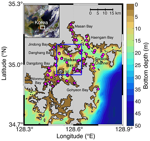
Figure 1. Study area and field station locations in Jinhae Bay, Korean Peninsula. Inset map shows the GOCI RGB color composite (680/555/412 nm) image on 20 May 2015, processed using the GDPS. Purple circles mark the locations of the in situ Chl-a observations. The blue box marks the area subjected to the time series analysis presented in Figure 8. The color bar represents the bottom topography (m) from the ETOPO1 (Amante and Eakins, 2009).

Since the 1970s, intensive anthropogenic activities in this area have discharged domestic sewage and land-use wastes (3,800 and 3,600 kg d⁻¹, respectively) into several inflowing streams (Lee et al., 2018), loading them with massive nutrient contents (Lee and Min, 1990). These characteristics have resulted in serious environmental problems, such as eutrophication, hypoxia, and harmful algal blooms (red tides), leading to significant changes in coastal biogeochemical cycles and ecosystem structures (Lee and Lim, 2006; Moon et al., 2008; Kim D. et al., 2012; Lee et al., 2017; Lim et al., 2018). Hence, coastal ecosystem conservation in this area has become an important socioeconomic and scientific issue, and there have been many calls for a coastal ecosystem monitoring and effective water quality management systems.

The Geostationary Ocean Color Imager (GOCI), the world's first geostationary ocean color satellite, was launched in June 2010 to monitor short- and long-term changes in marine ecosystems around the Korean Peninsula (Figure 1; Cho et al., 2010). GOCI provides ocean color products, such as remote sensing reflectance (R_rs), chlorophyll-a concentration (Chl-a), and TSM, in near real-time during the daytime, from 09:16 to 16:16 local time (a total of eight images per day), and at a high spatial resolution of 500 m (Ryu et al., 2011; Choi et al., 2012). The Chl-a product is widely used as a primary variable for water quality assessment because it is an indicator of phytoplankton biomass, which is an important component of all marine ecosystems (Vaiciute et al., 2012). Therefore, GOCI-derived Chl-a can be monitored to track ecosystem dynamics and assess the temporal and spatial changes in coastal water quality around the Korean Peninsula in near real-time.

However, the estimation of Chl-a from ocean color satellites remains a challenging task in coastal waters, generally classified as Case-2 waters, where the optical properties are influenced not only by phytoplankton but also by other water constituents, such as TSM and/or colored dissolved organic matter (CDOM) (Morel and Prieur, 1977; Gordon and Morel, 1983; Tassan, 1994; Bukata et al., 1995; IOCCG, 2000; Ruddick et al., 2001; Pradhan et al., 2005; Siswanto et al., 2011; Tilstone et al., 2013). Therefore, a regionally optimized Chl-a algorithm must be applied to coastal waters by evaluating and tuning the Chl-a retrieval algorithms (Gitelson et al., 1996; Garcia et al., 2005; Hattab et al., 2013).

To date, several Chl-a algorithms have been developed and evaluated for Korean waters (Moon et al., 2010; Siswanto et al., 2011; Kim W. et al., 2016). The first validation of GOCI-derived Chl-a estimates, based on the NASA global standard algorithms (O'Reilly et al., 2000) and regional algorithms developed for Korean waters (Moon et al., 2010; Siswanto et al., 2011), was performed using in situ data collected from near-shore coastal waters around the Korean Peninsula (Moon et al., 2012). This validation showed that these Chl-a algorithms were not suitable for Korean coastal waters because of the diverse bio-optical properties of these regions. Subsequently, Kim W. et al. (2016) evaluated the Chl-a estimates from GOCI data obtained by applying newly derived coefficients of Chl-a algorithms for three turbidity levels, in reference to in situ data collected at 491 stations around the Korean Peninsula between 2010 and 2014. However, no Chl-a measurements from Jinhae Bay were involved in evaluation of the algorithms. Furthermore, no satellite-based study has yet focused on Jinhae Bay.

Therefore, the purpose of this study is to evaluate the GOCI-derived Chl-a estimates for Jinhae Bay obtained by two global open ocean algorithms and four regional algorithms for Korean waters, in reference to in situ Chl-a measurements from 2011 to 2016. We aim to provide a baseline approach for a GOCI-based long-term monitoring system that can produce accurate assessments and enable effective management of Jinhae Bay's coastal ecosystem and water quality, which is an area showing rapidly increasing anthropogenic activities.

Data and Methods

In situ Data

Surface water samples (<1-m depth) were collected using a 5-L Niskin bottle (standard model 110, OceanTest Equipment Inc., https://www.oceantestequip.com/) with monthly to bi-monthly intervals between 2011 and 2016 at 54 stations in Jinhae Bay (n = 1688) as part of the coastal environmental monitoring program of the National Institute of Fisheries Science (NIFS), Korea (Figure 1). Chl-a samples were immediately collected by filtering 500-mL of surface seawaters onto 25-mm-diameter nitrocellulose filters. The filter papers were stored in the dark at −20°C before laboratory analysis. In the laboratory, Chl-a was extracted with 15-ml of 90% acetone for 24 h as described in EPA Method 445.0 (Knap et al., 1996; U.S. EPA., 1997a), and the Chl-a concentrations were then measured with a 10-AU fluorometer (Turner Designs, CA, USA; Welschmeyer, 1994). The fluorometer was calibrated with a standard Chl-a solution once a year and its calibration status was checked with the solid secondary standard material prior to each series of measurements. For the TSM analysis, 500-mL water samples were filtered through 47-mm-diameter GF/F filters, which were weighed prior to filtering and then reweighed after filtering and drying; the TSM was calculated as the difference between the initial and final weights. The diffuse attenuation coefficient (K_d) was derived from the Secchi depth, measured with a white 30-cm-diameter disk (Holmes, 1970). Salinity was determined from the conductivity and temperature readings by temperature/conductivity probe mounted on an YSI 6600 V2 Sonde (Yellow Springs Instruments, USA). Water sample for nitrate analysis was immediately filtered (0.45 μm, Millipore membrane syringe filter) directly into a vial and stored at −20°C. Nitrate was determined using the flow injection analysis system (QuAAtro, Seal Analytical) by cadmium reduction methods (U.S. EPA., 1997b). Total nitrogen was measured through determination of nitrate concentration after persulphate oxidation of non-filtered water sample (Grasshoff, 1983).

GOCI R_rs Data

GOCI L1B data (500 × 500 m resolution), covering the time period and locations of the in situ measurements, were downloaded from the Korea Ocean Satellite Center (KOSC) website (http://kosc.kiost.ac.kr). These L1B images were processed to L2 R_rs data at six wavelength bands (412, 443, 490, 555, 660, and 680 nm) using the GOCI Data Processing System (GDPS, version 2.0), which implements the KOSC standard atmospheric correction algorithm. Only GOCI R_rs values acquired at 12:16 local time were used to avoid the influence of the solar zenith angle (Hooker and McClain, 2000).

Ocean Color Chl-a Algorithms

Six algorithms (two OCxS algorithms for the open ocean, one GOCI-standard algorithm, and three Tassan's algorithms regionally modified for Korean waters) were selected to assess the GOCI-derived Chl-a estimates in Jinhae Bay (Moon et al., 2010; NASA, 2010; Siswanto et al., 2011; Kim W. et al., 2016).

The OCxS algorithms were developed as the operational algorithms for NASA's Sea-Viewing Wide Field-of-view Sensor (SeaWiFS). They use a fourth-order polynomial relationship between the ratio of R_rs (i.e., blue-green band ratio) and Chl-a (NASA, 2010). In this study, we tested two OCxS algorithms: OC2S and OC3S.

OC2S uses the two-band ratio (NASA, 2010), given as

$\begin{array}{ll}{\text{Chl}-\text{a}=10}^{0.2511-2.0853R+1.5035R^2-3.1747R^3+0.3383R^4},& (1)\end{array}$

where

$\begin{array}{ll}R={\text{log}}_{\text{10}}\frac{R_{rs}\left(490\right)}{R_{rs}\left(555\right)}.& (2)\end{array}$

OC3S uses the three-band ratio (NASA, 2010), given as

$\begin{array}{ll}\text{Chl}-\text{a}={10}^{0.2515-2.3798R+1.5823R^2-0.6372R^3-0.5692R^4},& (3)\end{array}$

where

$\begin{array}{ll}R={\text{log}}_{\text{10}}\frac{\max \left(R_{rs}\left(443\right),R_{rs}\left(490\right)\right)}{R_{rs}\left(555\right)}.& (4)\end{array}$

As the regional algorithm for Korean waters, we first tested the GOCI-standard Chl-a algorithm, developed for GOCI products using in situ Chl-a data collected around the Korean Peninsula from 1998 to 2009 (Moon et al., 2010). The GOCI-standard is given as

$\begin{array}{ll}\text{Chl}-\text{a}=1.8528R^{-3.263},& (5)\end{array}$

where

$\begin{array}{ll}R=\frac{(R_{rs}(443)+R_{rs}(490))-R_{rs}(412)}{R_{rs}(555)}.& (6)\end{array}$

Tassan's algorithm, developed for turbid waters (Tassan, 1994), was regionally optimized as the Yellow Sea Large Marine Ecosystem Ocean Color Project (YOC) algorithm, using in situ Chl-a measurements from the Yellow Sea and East China Sea acquired between 1998 and 2007 (Siswanto et al., 2011). The YOC algorithm is given as

$\begin{array}{ll}{\text{Chl}-\text{a}=10}^{0.342-2.511R-0.277R^2},& (7)\end{array}$

where

$\begin{array}{ll}R={\text{log}}_{\text{10}}\frac{R_{rs}\left(443\right)}{R_{rs}\left(555\right)}{\left[\frac{R_{rs}\left(412\right)}{R_{rs}\left(490\right)}\right]}^{-1.012}.& (8)\end{array}$

Kim W. et al. (2016) modified Tassan's algorithm for the GOCI product by using in situ data (2010–2014) collected from coastal areas around the Korean Peninsula, East China Sea, and Tsushima Strait. This modification, termed Tassan-All, is given as

$\begin{array}{ll}{\text{Chl}-\text{a}=10}^{-0.0751-1.7156R-0.1119R^2},& (9)\end{array}$

where

$\begin{array}{ll}R={\text{log}}_{\text{10}}\frac{R_{rs}\left(443\right)}{R_{rs}\left(555\right)}{\left[\frac{R_{rs}\left(412\right)}{R_{rs}\left(490\right)}\right]}^{-0.5093}.& (10)\end{array}$

Kim W. et al. (2016) also modified regionally the coefficients of Tassan's algorithm, applying different coefficients for three TSM levels: low TSM of 0–0.5 g m⁻³ or R_rs(555) <0.004 sr⁻¹ (Tassan-LS); moderate TSM of 0.5–10 g m⁻³ or R_rs(555) of 0.004–0.015 sr⁻¹ (Tassan-MS); and high TSM of >10 g m⁻³ or R_rs(555) >0.015 sr⁻¹ (Tassan-HS). The three modifications are referred to collectively as the Tassan-TD algorithm.

The Tassan-LS algorithm is given as

$\begin{array}{ll}{\text{Chl}-\text{a}=10}^{-0.0509-1.6888R-0.1497R^2},& (11)\end{array}$

where

$\begin{array}{ll}R={\text{log}}_{\text{10}}\frac{R_{rs}\left(443\right)}{R_{rs}\left(555\right)}{\left[\frac{R_{rs}\left(412\right)}{R_{rs}\left(490\right)}\right]}^{-0.4404}.& (12)\end{array}$

The Tassan-MS algorithm is given as

$\begin{array}{ll}{\text{Chl}-\text{a}=10}^{0.1235-1.6072R+4.6815R^2},& (13)\end{array}$

where

$\begin{array}{ll}R={\text{log}}_{\text{10}}\frac{R_{rs}\left(443\right)}{R_{rs}\left(555\right)}{\left[\frac{R_{rs}\left(412\right)}{R_{rs}\left(490\right)}\right]}^{-1.0138}.& (14)\end{array}$

The Tassan-HS algorithm is given as

$\begin{array}{ll}{\text{Chl}-\text{a}=10}^{-0.2318-1.1292R+2.6650R^2},& (15)\end{array}$

where

$\begin{array}{ll}R={\text{log}}_{\text{10}}\frac{R_{rs}\left(443\right)}{R_{rs}\left(555\right)}{\left[\frac{R_{rs}\left(412\right)}{R_{rs}\left(490\right)}\right]}^{-0.2307}.& (16)\end{array}$

Match-up Procedure

GOCI R_rs values were extracted for a 5 × 5-pixel window centered on the location of the in situ sample for comparison. The maximum temporal difference between the GOCI and in situ measurements was set at 4 h. The following GOCI L2 flags rendered a pixel invalid for the matching analysis: cloud or ice, land, atmospheric correction failure, unrealistic R_rs spectrum shape, out of GOCI observation boundary, high solar zenith angle (>70°), high satellite zenith angle (>55°), cloud edge, bright pixel adjacency warning, Chl-a failure (not calculable), or Chl-a warning (Chl-a >1,300 mg m⁻³). The inter-slot radiometric discrepancy was not corrected in this study because this flag was not yet implemented in GDPS. We then calculated the mean and standard deviation (SD) of the 25 pixels and deleted those pixels with values outside the range of the mean ± 1.5 SD (Bailey and Werdell, 2006). The mean R_rs value of all valid pixels within the 5 × 5-pixel window was used for the comparisons. We accepted only matched pairs with mean R_rs values above zero at all six wavelength bands. The final number of matched pairs was 22.

Statistical Analysis

The performances of the tested algorithms were evaluated based on the following statistical parameters: Pearson's correlation coefficient (r), slope (S) and intercept (I) of Type-2 linear regression (York, 1966; Laws and Archie, 1981; Glover et al., 2011) fitted on log-transformed Chl-a data; root-mean-square error (RMSE, Δ); bias (δ); and mean ratio. The latter three parameters are defined, respectively, as

$\begin{array}{ll}\Delta =\sqrt{\frac{1}{n}{\sum }_{i=1}^n{(y_i-x_i)}^2},& (17)\end{array}$

$\begin{array}{ll}\delta =\frac{1}{n}{\sum }_{i=1}^n(y_i-x_i),& (18)\end{array}$

and

$\begin{array}{ll}\text{mean ratio}=\frac{1}{n}{\sum }_{i=1}^n\frac{y_i}{x_i},& (19)\end{array}$

where x_i and y_i denote the in situ Chl-a data and corresponding GOCI-derived Chl-a estimates for the i-th matched pair, respectively, and n is the number of matched pairs.

Outliers are defined as GOCI-derived Chl-a estimates that fall outside the range from 1/20 to 20 times the in situ Chl-a. Outlier points were removed from the matching analysis for each algorithm (Pitarch et al., 2016).

Results and Discussion

Spatiotemporal Variability of the Chlorophyll-a Measurements

The in situ Chl-a measurements (n = 1688), ranging between 0.014 mg m⁻³ and 162.1 mg m⁻³, exhibited a log-normal distribution (Figure 2A). The median and mean values of Chl-a were 3.0 and 6.5 mg m⁻³, respectively.

FIGURE 2

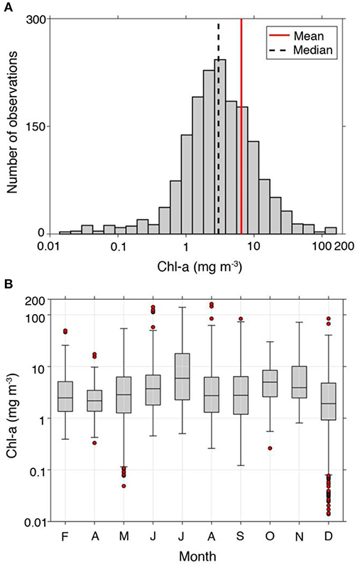
Figure 2. In situ Chl-a observations. (A) Histograms of in situ Chl-a (mg m⁻³). The black dashed and red solid lines indicate median and mean values, respectively. (B) Box plot of monthly in situ Chl-a (mg m⁻³) for the study period (2011–2016). Box plot in (B) depicts median (horizontal line), interquartile range (box), 1.5 × interquartile range (error bars), and outliers (red dots) that fall more than 1.5 times the interquartile range below the first quartile or above the third quartile.

Chl-a was seasonally lower during the winter months (December and February; median value = 2.2 mg m⁻³) and showed a gradually increasing trend in spring months (April and May; median value = 2.4 mg m⁻³; Figure 2B). The monthly mean Chl-a value was highest in July (mean ± SD = 15.6 ± 23.6 mg m⁻³). Overall, the Chl-a values showed a positive correlation with the total nitrogen (r = 0.5, p < 0.05), whereas had a negative correlation with the salinity (r = −0.4, p < 0.05), which were collected from the same NIFS cruises during the study period (NIFS, 2012, 2013, 2014, 2015, 2016, 2017). This result indicates that the Chl-a dynamics in the Jinhae Bay were likely to be associated with the supply of nitrogen via low salinity waters. In particular, the maximum of monthly mean Chl-a values occurred in July 2011 (31.5 ± 30.9 mg m⁻³; NIFS, 2012), corresponding to the highest nitrate concentration (32.8 ± 24.4 μM) and the lowest salinity (18.0 ± 5.2) caused by heavy precipitation (http://www.kma.go.kr/). Previous studies reported that large phytoplankton blooms in Jinhae Bay occurred during the summer months (June through August) resulted from the high nutrient loadings associated with increased summer precipitation (accounting for ~60% of annual precipitation; Baek and Kim, 2010; Baek et al., 2012; Park et al., 2012; Kim et al., 2013). These massive nutrient loadings have frequently caused outbreak of red tides in this area (Kwak et al., 2001). Seasonal secondary bloom occurred in October (6.5 ± 5.5 mg m⁻³) as stratification became weak (Kim et al., 2015; Lim et al., 2018), and this bloom remained until November (8.4 ± 11.9 mg m⁻³; Figure 2B). In December, Chl-a showed a seasonal minimum value (median value = 1.9 mg m⁻³) with a large range from 0.014 to 84.5 mg m⁻³.

The spatial distribution of monthly mean Chl-a values (Figure 3A) showed that relatively higher Chl-a concentrations occurred nearly all year in the northeastern regions of Jinhae Bay, where high nutrient loadings occur through a number of small streams proximate to industrial complexes and cities (Cho and Chae, 1998; Jeong et al., 2006), whereas relatively lower Chl-a concentrations were found in the southwestern regions (Kim et al., 2013, 2014; Lee et al., 2018). The seasonal and regional Chl-a distribution patterns were similar to the TSM and K_d distributions, which also exhibited their highest values in July in the northeastern region of Jinhae Bay (Figure 3).

FIGURE 3

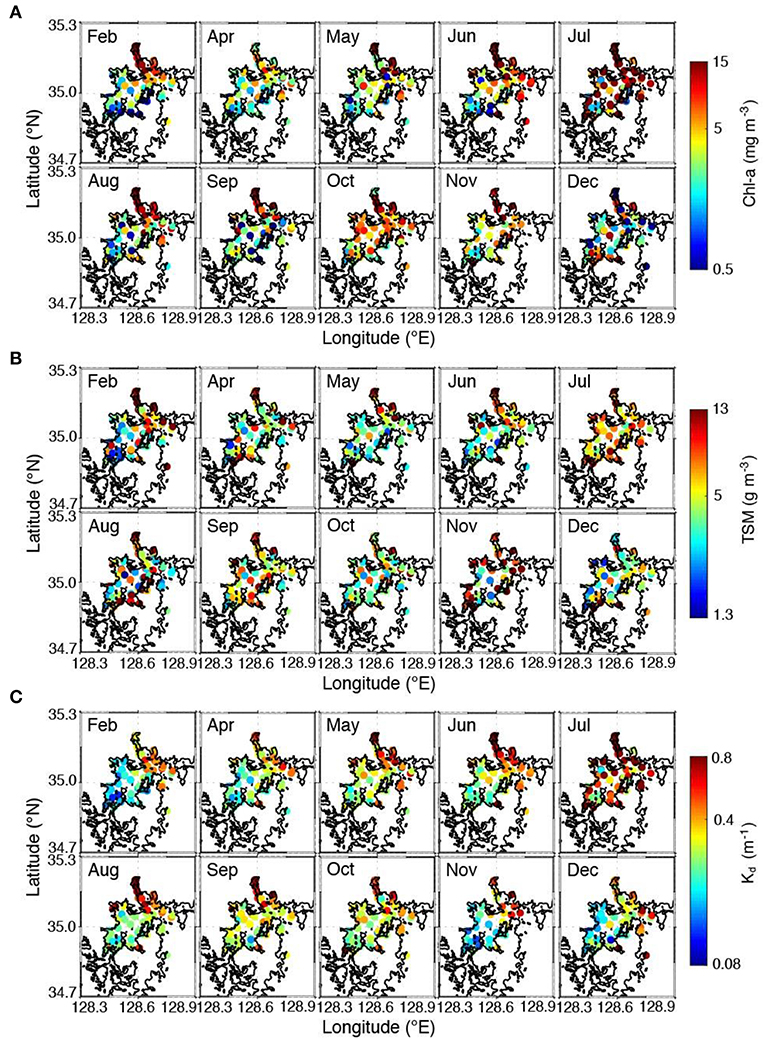
Figure 3. Monthly spatial distribution of (A) in situ Chl-a (mg m⁻³), (B) in situ TSM (g m⁻³), and (C) in situ K_d (m⁻¹).

To determine whether light attenuation in Jinhae Bay was directly related to phytoplankton biomass, we analyzed the relationship between Chl-a and K_d, as well as between TSM and K_d. The K_d values were positively correlated with both TSM (r = 0.4, p < 0.05, n = 1652) and Chl-a (r = 0.6, p < 0.05, n = 1684; Figure 4), suggesting that the variability in light penetration in Jinhae Bay was determined not only by increases in phytoplankton biomass, but also by changes in TSM. A mean K_d value of 0.36 m⁻¹ (range: 0.08–2.88 m⁻¹) was observed, which was similar to that of the coastal waters along the Gujarat coast and Gulf of Kachchh, India (>0.15 m⁻¹; Sarangi et al., 2002). The TSM concentrations ranged from 0.6 to 72.8 g m⁻³, with a mean value of 6.4 g m⁻³; this range was comparable to the ranges of moderate and high levels of TSM in the in situ datasets used to develop the Tassan-TD algorithm (Kim W. et al., 2016). These results indicate that Jinhae Bay represents the Case-2 waters, the optical properties of which are influenced by phytoplankton (Gordon and Morel, 1983; Bukata et al., 1995; IOCCG, 2000) and a number of other optical components (e.g., TSM).

FIGURE 4

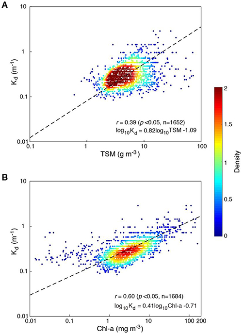
Figure 4. Density scatter plots showing the relationship between in situ K_d (m⁻¹) and: (A) in situ TSM (g m⁻³) and (B) in situ Chl-a (mg m⁻³). The black dotted line is the best-fit linear regression line for all the data in each comparison. The color bar marks density.

Comparison of the Performance of Ocean Color Chl-a Algorithms

The atmospheric correction strategies applied can introduce large uncertainties and variability in remote sensing data from optically complex coastal waters (Gordon and Wang, 1994; IOCCG, 2000). For example, Siswanto et al. (2011) showed that the performance of the YOC algorithm as applied to the SeaWiFS data was relatively poor because of improper atmospheric corrections, based on a comparative analysis of the SeaWiFS and in situ R_rs data, whereas an improved atmospheric correction resulted in the improved performance of ocean color algorithms over coastal waters (Zhang et al., 2010; Siswanto et al., 2011). Kim W. et al. (2016) also reported that the overestimation of GOCI R_rs in the blue bands (412, 443, and 490 nm), which is related to the atmospheric correction, may have caused underestimation of in situ Chl-a values >1.5 mg m⁻³ with moderate and high TSM levels.

In order to investigate the impact of the atmospheric correction algorithm on Chl-a estimates, therefore, we compared the R_rs data derived from the KOSC atmospheric correction algorithm with those derived from the NASA atmospheric correction algorithm for Jinhae Bay (Supplementary Text 1; Supplementary Figure 1). The comparison of the GOCI R_rs values derived from the KOSC and NASA atmospheric correction algorithms, respectively, showed that the R_rs values at the blue bands were scattered more than those at the green band (555 nm; Supplementary Figure 1). The R_rs values at the blue bands derived from the NASA algorithm were lower than those derived from the KOSC algorithm, showing especially large biases in R_rs values at 412 nm. Although the development of KOSC atmospheric correction algorithm was based on the global NASA algorithm (Bailey et al., 2010), the KOSC algorithm has been partially updated for turbid Case-2 water corrections (Ahn et al., 2012) and adjusted for vicarious calibration gains (Ahn et al., 2015) and aerosol correction schemes (Gordon and Wang, 1994; IOCCG, 2010; Ahn et al., 2016, 2018), indicating that the KOSC algorithm is likely to be more suitable to estimate local/regional Chl-a estimation in this study.

To evaluate the performances of the six ocean color Chl-a algorithms applied to the KOSC-GOCI R_rs data from Jinhae Bay, we first constructed histograms of both the in situ and GOCI-derived Chl-a values in matched datasets (Figure 5). The distributions of the in situ and GOCI-derived Chl-a values both followed an approximately log-normal distribution. The GOCI-standard and YOC Chl-a algorithms showed similar ranges in their Chl-a estimates relative to the corresponding in situ Chl-a values (Figures 5C,D). However, the histograms of the GOCI-derived Chl-a estimates obtained using the OC2S, OC3S, Tassan-All, and Tassan-TD Chl-a algorithms showed distributions shifted to the left, with relatively lower mean values for the Chl-a estimates (mean range: 0.7–1.0 mg m⁻³) compared to the in situ Chl-a values (2.7 ± 1.9 mg m⁻³; Figures 5A,B,E,F).

FIGURE 5

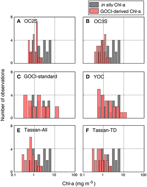
Figure 5. Histograms of in situ Chl-a (gray bars) and GOCI-derived Chl-a obtained using the following six algorithms (red bars): (A) OC2S, (B) OC3S, (C) GOCI-standard, (D) YOC, (E) Tassan-All, and (F) Tassan-TD.

As shown in Figure 6, scatter plots of in situ Chl-a vs. GOCI-derived Chl-a estimates from the six ocean color Chl-a algorithms, most of the tested Chl-a algorithms overestimated the in situ Chl-a values (<0.8 mg m⁻³), except for Tassan-All. For high in situ Chl-a values (>0.9 mg m⁻³), the GOCI-derived Chl-a estimates from all algorithms generally underestimated the results. The GOCI-derived Chl-a values from the OC2S, OC3S, Tassan-All, and Tassan-TD algorithms ranged from 0.2 to 2.4 mg m⁻³, compared to the high in situ Chl-a value range from 0.9 to 6.8 mg m⁻³ (Figures 6A,B,E,F). This underestimation of high Chl-a values was comparable to the previously reported tendency of the Chl-a algorithm validation results from GOCI products for Korean coastal waters (Moon et al., 2010, 2012; Kim W. et al., 2016). However, overall the GOCI-derived Chl-a estimates from the YOC algorithm were distributed appropriately around the 1:1 line for in situ Chl-a values (Figure 6D) and also its mean ratio was close to one, indicating that the YOC algorithm yielded the most significant correlation (r = 0.51, p < 0.05) between the in situ and GOCI-derived Chl-a values (Table 1). Moreover, the YOC algorithm exhibited the bias (δ = 0.03) closest to zero and a relatively low error (△ = 2.52), compared to the other algorithms. As a result of statistical analysis, the YOC algorithm performed best for the Jinhae Bay Chl-a estimations.

FIGURE 6

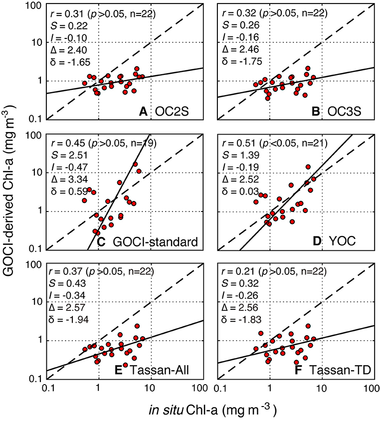
Figure 6. Scatter plots between in situ Chl-a and GOCI-derived Chl-a for the six algorithms: (A) OC2S, (B) OC3S, (C) GOCI-standard, (D) YOC, (E) Tassan-All, and (F) Tassan-TD. The dashed and solid black line mark the 1:1 line and the Type-2 linear regression fit, respectively.

TABLE 1

Table 1. Statistical results for the matched pairs in Jinhae Bay.

The performances of the Chl-a retrieval algorithms were also evaluated by comparing the spatial distributions of in situ and GOCI-derived Chl-a averages from two sampling periods, April 4–7, 2014 (Figure 7A) and August 3–4 and 6–7, 2016 (Figure 7B). The spatial distributions of the GOCI-derived Chl-a values were calculated using the six Chl-a algorithms, excluding only low-quality pixels that were flagged as cloud or ice, land, atmospheric correction failure, unrealistic R_rs spectrum shape, out of GOCI observation boundary, high solar zenith angle (>70°), high satellite zenith angle (>55°), or cloud edge. Except for the GOCI-standard and YOC algorithms, all Chl-a algorithms tested estimated relatively lower Chl-a values compared to the in situ data, showing especially strong tendencies to underestimate Chl-a values for summer (August 3–4 and 6–7, 2016), when Chl-a concentrations were relatively higher. Although Chl-a estimates from the GOCI-standard algorithm showed a spatial distribution comparable to the in situ Chl-a values obtained for the spring period, the GOCI-standard algorithm overestimated the Chl-a values for the summer period when in situ Chl-a values were relatively higher than in the spring period. However, the in situ Chl-a averages from the two sampling periods both showed that spatial distribution patterns were similar to those estimated using the YOC algorithm, showing relatively higher values in areas near Gadeok Channel (~2 mg m⁻³ in 2014 and ~5 mg m⁻³ in 2016, respectively) and relatively lower values around Gajo island (~1 mg m⁻³ in 2014 and ~2 mg m⁻³ in 2016, respectively).

FIGURE 7

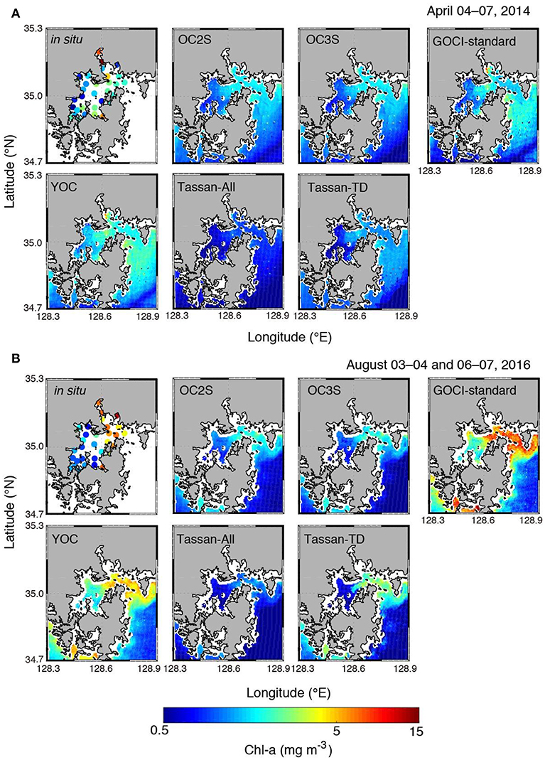
Figure 7. Spatial distribution of in situ Chl-a (mg m⁻³) and GOCI-derived Chl-a from six algorithms averaged for two sampling periods: (A) April 4–7, 2014 and (B) August 3–4 and 6–7, 2016, respectively. We excluded pixels with extreme concentrations (Chl-a <0.001 mg m⁻³ or Chl-a >500 mg m⁻³) and low-quality L2 data flagged as cloud or ice, land, atmospheric correction failure, unrealistic R_rs spectrum shape, out of GOCI observation boundary, high solar zenith angle (>70°), high satellite zenith angle (>55°), or cloud edge from the analysis.

To further evaluate the accuracy of the YOC algorithm as applied to the Jinhae Bay data, the YOC algorithm was applied to GOCI R_rs data obtained over the 2011–2016 period. The flags applied to this analysis were the same as those applied to the spatial analysis. Temporal patterns were analyzed based on the average value for the blue box area shown in Figure 1 (34.95°N−35.1°N and 128.5°E−128.65°E). The area-averaged daily time series of in situ Chl-a values from 2011 to 2016 was compared with the GOCI-derived Chl-a values obtained using the YOC algorithm (Figure 8). The daily in situ Chl-a values varied from 0.03 to 56.1 mg m⁻³, whereas the GOCI-derived Chl-a values from YOC algorithm varied from 0.04 to 130.2 mg m⁻³. The YOC algorithm generally slightly underestimated the Chl-a values compared to the in situ Chl-a values (Figure 8). Nonetheless, the slight discrepancies did not inhibit the YOC algorithm's reasonable representations of the seasonal variation of the in situ data.

FIGURE 8

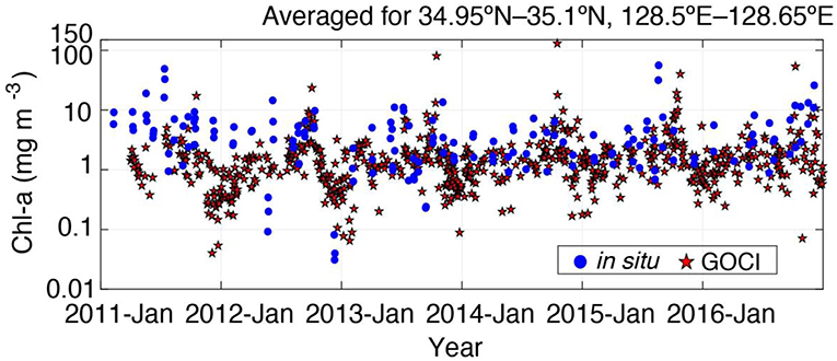
Figure 8. Time series of the in situ Chl-a values (blue circles) and GOCI-derived Chl-a estimates from the YOC algorithm (red stars), averaged for the blue box area shown in Figure 1 (34.95°N−35.1°N and 128.5°E−128.65°E). Pixel exclusion criteria were the same as in Figure 7.

In summary, the YOC algorithm showed a statistically significant correlation with in situ Chl-a values from Jinhae Bay (Figure 6D; Table 1). The spatial distribution of the GOCI-derived Chl-a estimates from the YOC algorithm was also closest to that of the in situ Chl-a values (Figure 7). Furthermore, the daily time series of the in situ Chl-a values was agreed well with the GOCI-derived Chl-a values obtained using YOC algorithm, showing the distinctive seasonal variations (Figure 8). Therefore, the YOC algorithm will enable monitoring of ecosystem responses to anthropogenic impacts with near real time in the Jinhae Bay.

Suggestions for Future Research

In this study, the evaluation of the Chl-a algorithms was performed using only in situ Chl-a measurements, without considering in situ R_rs measurements from Jinhae Bay, which inhibited the validation of the atmospheric correction and the development and assessment of a regionally optimized Chl-a algorithm based on in situ R_rs data from Jinhae Bay. Therefore, further work should be done to assess the atmospheric correction results of the GOCI R_rs data at the blue bands based on in situ R_rs measurements from Jinhae Bay. Such assessments would enable the development of new atmospheric correction algorithms optimized for coastal waters, perhaps including algorithms based on a multilayer neural network (Fan et al., 2017), with the final objective of developing a regionally optimized Chl-a algorithm for the GOCI R_rs products in Jinhae Bay. Raman scattering effects may also need to be considered to develop regional Chl-a algorithms because Raman fractions can contribute ~8% in R_rs at 555 nm in Case-2 waters (Gupta, 2015). These future works will thus yield a more accurate refinement of our GOCI-derived approach.

Conclusion

In order to provide a baseline approach to satellite-based coastal monitoring of the eutrophic Jinhae Bay environment in near real-time, we compared the GOCI-derived Chl-a estimates from two global open ocean algorithms and four regional algorithms with in situ Chl-a measurements between 2011 and 2016. Among the six tested ocean color algorithms, the YOC algorithm yielded the best performance results, producing Chl-a estimates closer to the 1:1 line compared to the other algorithms and spatial patterns similar to the in situ Chl-a values. Time series analyses of the in situ and GOCI-derived Chl-a values also agreed well, with the YOC algorithm detecting seasonal variations similar to those measured. Although the GOCI-derived Chl-a values from YOC algorithm showed the best fit to the in situ values from Jinhae Bay, this algorithm nonetheless yielded biased estimates (e.g., a slight underestimation of high in situ Chl-a values >~1.0 mg m⁻³). Hence, a Chl-a algorithm regionally optimized for Jinhae Bay must be further developed by collecting in situ R_rs data, which would enhance the opportunity to monitor eutrophication associated with anthropogenic activities in near real-time across Jinhae Bay by providing a more accurate Chl-a estimation.

Author Contributions

J-EY and I-NK developed the idea and wrote the manuscript. J-EY, J-HL, SS, S-HY, H-JO, J-DH, J-IK, and S-SK conducted the literature survey and analysis. All the authors discussed and approved the final manuscript.

Conflict of Interest Statement

The authors declare that the research was conducted in the absence of any commercial or financial relationships that could be construed as a potential conflict of interest.

Acknowledgments

This work was supported by Research on the characteristics of marine ecosystem and oceanographic observation in Korean waters (R2019041). This research was a part of the project titled Improvements of ocean prediction accuracy using numerical modeling and artificial intelligence technology, funded by the Ministry of Oceans and Fisheries, Korea. This work was also supported by the National Research Foundation of Korea (NRF) grant funded by the Korea government (MSIT) (NRF-2019R1F1A1051790). Thanks to the KOSC staff and NASA's Ocean Biology Processing Group for providing GOCI data used in this study.

Supplementary Material

The Supplementary Material for this article can be found online at: https://www.frontiersin.org/articles/10.3389/fmars.2019.00359/full#supplementary-material

References

Ahn, J.-H., Park, Y.-J., and Fukushima, H. (2018). Comparison of aerosol reflectance correction schemes using two near-infrared wavelengths for ocean color data processing. Remote Sens. 10:1791. doi: 10.3390/rs10111791

CrossRef Full Text | Google Scholar

Ahn, J.-H., Park, Y.-J., Kim, W., and Lee, B. (2016). Simple aerosol correction technique based on the spectral relationships of the aerosol multiple-scattering reflectances for atmospheric correction over the oceans. Opt. Express. 24, 29659–29669. doi: 10.1364/OE.24.029659

CrossRef Full Text | Google Scholar

Ahn, J.-H., Park, Y.-J., Kim, W., Lee, B., and Oh, I. S. (2015). Vicarious calibration of the geostationary ocean color imager. Opt. Express. 23, 23236–23258. doi: 10.1364/OE.23.023236

PubMed Abstract | CrossRef Full Text | Google Scholar

Ahn, J.-H., Park, Y.-J., Ryu, J. H., Lee, B., and Oh, I. S. (2012). Development of atmospheric correction algorithm for Geostationary Ocean Sci. J. 47, 247–259. doi: 10.1007/s12601-012-0026-2

CrossRef Full Text | Google Scholar

Amante, C., and Eakins, B. W. (2009). ETOPO1 1 Arc-Minute Global Relief Model: Procedures, Data Sources and Analysis. NOAA Technical Memorandum NESDIS NGDC-24. National Geophysical Data Center, NOAA.

Google Scholar

Bae, H., Lee, J.-H., Song, S. J., Park, J., Kwon, B.-O., Hong, S. S., et al. (2017). Impacts of environmental and anthropogenic stresses on macrozoobenthic communities in Jinhae Bay, Korea. Chemosphere 171, 681–691. doi: 10.1016/j.chemosphere.2016.12.112

PubMed Abstract | CrossRef Full Text | Google Scholar

Baek, S.-H., Son, M., Hyun, B.-G., Kim, D.-S., Choi, H.-W., and Kim, Y.-O. (2012). The correlation between environmental factors and phytoplankton communities in spring and summer stratified water-column at Jinhae Bay, Korea. Korean J. Environ. Biol. 30, 219–230.

Google Scholar

Baek, S. H., and Kim, Y. O. (2010). The Study of summer season in Jinhae Bay-Short-term changes of community structure and horizontal distribution characteristics of phytoplankton. Korean J. Environ. Biol. 28, 115–124.

Google Scholar

Bailey, S. W., Franz, B. A., and Werdell, P. J. (2010). Estimation of near-infrared water-leaving reflectance for satellite ocean color data processing. Optics Express 18, 7521–7527. doi: 10.1364/OE.18.007521

PubMed Abstract | CrossRef Full Text | Google Scholar

Bailey, S. W., and Werdell, P. J. (2006). A multi-sensor approach for the on-orbit validation of ocean color satellite data products. Remote Sens. Environ. 102, 12–23. doi: 10.1016/j.rse.2006.01.015

CrossRef Full Text | Google Scholar

Bukata, R. P., Jerome, J. H., Kondratyev, A. S., and Pozdnyakov, D. V. (1995). Optical Properties and Remote Sensing of Inland and Coastal Waters. Boca Raton, FL: CRC Press.

Google Scholar

Cho, H.-Y., and Chae, J.-W. (1998). Analysis on the Characteristics of the Pollutant Load in Chinhae-Masan Bay. Korean Soc. Coast. Ocean Eng. 10, 132–140.

Google Scholar

Cho, H. Y., Chae, J. W., and Chun, S. Y. (2002). Stratification and DO concentration change in Chinhae-Masan Bay. J. Korean Soc. Coast. Ocean. Eng. 14, 295–307.

Google Scholar

Cho, K.-J., Choi, M.-Y., Kwak, S.-K., Im, S.-H., Kim, D.-Y., Park, J., et al. (1998). Eutrophication and seasonal variation of water quality in masan-Jinhae Bay. Sea 3, 193–202.

Google Scholar

Cho, S., Ahn, Y. H., Ryu, J. H., Kang, G.-S., and Youn, H.-S. (2010). Development of Geostationary Ocean Color Imager (GOCI). Korean J. Remote Sens. 26, 157–165.

Google Scholar

Choi, J.-K., Park, Y. J., Ahn, J. H., Lim, H.-S., Eom, J., and Ryu, J.-H. (2012). GOCI, the world's first geostationary ocean color observation satellite, for the monitoring of temporal variability in coastal water turbidity. J. Geophys. Res. Oceans 117:C09004. doi: 10.1029/2012JC008046

CrossRef Full Text | Google Scholar

Fan, Y., Li, W., Gatebe, C. K., Jamet, C., Zibordi, G., Schroeder, T., et al. (2017). Atmospheric correction and aerosol retrieval over coastal waters using multilayer neural networks. Remote Sens. Environ. 199, 218–240. doi: 10.1016/j.rse.2017.07.016

CrossRef Full Text | Google Scholar

Garcia, C. A. E., Garcia, V. M. T., and McClain, C. R. (2005). Evaluation of SeaWiFS chlorophyll algorithms in the Southwestern Atlantic and Southern Oceans. Remote Sens. Environ. 95, 125–137. doi: 10.1016/j.rse.2004.12.006

CrossRef Full Text | Google Scholar

Gitelson, A., Karnieli, A., Goldman, N., Yacobi, Y. Z., and Mayo, M. (1996). Chlorophyll estimation in the Southeastern Mediterranean using CZCS images: adaptation of an algorithm and its validation. J. Mar. Syst. 9, 283–290. doi: 10.1016/S0924-7963(95)00047-X

CrossRef Full Text | Google Scholar

Glover, D. M., Jenkins, W. J., and Doney, S. C. (2011). Modeling Methods for Marine Science. Cambridge, UK: Cambridge University Press.

Google Scholar

Gordon, H. R., and Wang, M. (1994). Retrieval of water-leaving radiance and aerosol optical thickness over the oceans with SeaWiFS: a preliminary algorithm. Appl. Opt. 33, 443–452. doi: 10.1364/AO.33.000443

CrossRef Full Text | Google Scholar

Gordon, H. Y., and Morel, A. (1983). “Remote assessment of ocean color for interpretation of satellite visible imagery: a review,” in Lecture Notes on Coastal and Estuarine Studies, eds R. T. Barber, M. J. Bowman, C. N. K. Mooers et al. (New York, NY: Springer Verlag), 1–144. doi: 10.1029/LN004

CrossRef Full Text | Google Scholar

Grasshoff, K. (1983). “Determination of nitrate,”in Methods of Seawater Analysis. Second, Revised and Extended Edition, eds K. Grasshoff, M. Ehrhardt, and K. Kremling (Weinheim: Verlag Chemie).

Google Scholar

Gupta, M. (2015). Contribution of Raman scattering in remote sensing retrieval of suspended sediment concentration by empirical modeling. IEEE J. Sel. Top. Appl. Earth Obs. Remote Sens. 8, 398–405. doi: 10.1109/JSTARS.2014.2361336

CrossRef Full Text | Google Scholar

Hattab, T., Jamet, C., Sammari, C., and Lahbib, S. (2013). Validation of chlorophyll-α concentration maps from Aqua MODIS over the Gulf of Gabes (Tunisia): comparison between MedOC3 and OC3M bio-optical algorithms. Int. J. Remote Sens. 34, 7163–7177. doi: 10.1080/01431161.2013.815820

CrossRef Full Text | Google Scholar

Holmes, R. W. (1970). The secchi disk in turbid coastal waters. Limnol. Oceanogr. 15, 688–694. doi: 10.4319/lo.1970.15.5.0688

CrossRef Full Text | Google Scholar

Hooker, S., and McClain, C. (2000). The calibration and validation of SeaWiFS data. Prog. Oceanogr. 45, 427–465. doi: 10.1016/S0079-6611(00)00012-4

CrossRef Full Text | Google Scholar

IOCCG (2000). “Remote sensing of ocean colour in coastal, and other optically-complex, waters,” in Reports of the International Ocean-Colour Coordinating Group, ed S. Sathyendranath (Dartmouth: IOCCG).

Google Scholar

IOCCG (2010). “Atmospheric correction for remotely-sensed ocean-colour products,” in Reports of International Ocean-Colour Coordinating Group, ed M.Wang (Dartmouth: IOCCG).

Google Scholar

Jeong, K. S., Cho, J. H., Lee, J. H., and Kim, K. H. (2006). Accumulation history of anthropogenic heavy metals (cu, zn, and pb) in masan bay sediments, southeastern korea: a role of chemical front in the water column. Geosci. J. 10, 445–455. doi: 10.1007/BF02910438

CrossRef Full Text | Google Scholar

Kang, S. W. (1991). Circulation and pollutant dispersion in Masan-Jinhae Bay of Korea. Mar. Pollut. Bull. 23, 37–40. doi: 10.1016/0025-326X(91)90646-A

CrossRef Full Text | Google Scholar

Kim, D., Baek, S. H., Yoon, D. Y., Kim, K.-H., Jeong, J.-H., Jang, P.-G., et al. (2014). Water quality assessment at Jinhae Bay and Gwangyang Bay, South Korea. Ocean Sci. J. 49:251. doi: 10.1007/s12601-014-0026-5

CrossRef Full Text | Google Scholar

Kim, D., Choi, H. W., Choi, S. H., Baek, S. H., Kim, K. H., Jeong, J. H., et al. (2013). Spatial and seasonal variations in the water quality of Jinhae Bay, Korea. N. Z. J. Mar. Freshwater Res. 47, 192–207. doi: 10.1080/00288330.2013.772066

CrossRef Full Text | Google Scholar

Kim, D., Lee, C.-W., Choi, S.-H., and Kim, Y. O. (2012). Long-term changes in water quality of Masan Bay, Korea. J. Coast. Res. 2012, 923–929. doi: 10.2112/JCOASTRES-D-11-00165.1

CrossRef Full Text | Google Scholar

Kim, N. S., Kang, H., Kwon, M.-S., Jang, H.-S., and Kim, J. G. (2016). Comparison of seawater exchange rate of small scale inner bays within Jinhae Bay. J. Korean Soc. Mar. Environ. Energy 19, 74–85. doi: 10.7846/JKOSMEE.2016.19.1.74

CrossRef Full Text | Google Scholar

Kim, S.-Y., Lee, Y.-H., Kim, Y.-S., Shim, J.-H., Ye, M.-J., Jeon, J.-W., et al. (2012). Characteristics of marine environmental in the hypoxic season at Jinhae Bay in 2010. Korea J. Nat. Conserv. 6, 115–129. doi: 10.11624/KJNC.2012.6.2.115

CrossRef Full Text | Google Scholar

Kim, W., Moon, J.-E., Park, Y.-J., and Ishizaka, J. (2016). Evaluation of chlorophyll retrievals from Geostationary Ocean Color Imager (GOCI) for the North-East Asian region. Remote Sens. Environ. 184, 482–495. doi: 10.1016/j.rse.2016.07.031

CrossRef Full Text | Google Scholar

Kim, Y.-S., Lee, Y.-H., Kwon, J.-N., and Choi, H.-G. (2015). The effect of low oxygen conditions on biogeochemical cycling of nutrients in a shallow seasonally stratified bay in southeast korea (jinhae bay). Mar. Pollut. Bull. 95, 333–341. doi: 10.1016/j.marpolbul.2015.03.022

PubMed Abstract | CrossRef Full Text | Google Scholar

Knap, A., Michaels, A., Close, A., Ducklow, H., and Dickson, A. (1996). Protocols for the Joint Global Ocean Flux Study (JGOFS) Core Measurements. JGOFS Report Nr. 19, 170pp. Reprint of the IOC Manuals and Guides No. 29, UNESCO 1994.

Google Scholar

Kwak, S.-K., Choi, M. Y., and Cho, K.-J. (2001). Distribution and occurrence frequency of red-tide causing flagellates in the Masan-Jinhae Bay. Algae 16, 315–323.

Google Scholar

Laws, E. A., and Archie, J. W. (1981). Appropriate use of regression analysis in marine biology. Mar. Biol. 65, 13–16. doi: 10.1007/BF00397062

CrossRef Full Text | Google Scholar

Lee, C., and Lim, W. (2006). Variation of harmful algal blooms in Masan-Chinhae Bay. ScienceAsia 32(Suppl. 1), 51–56. doi: 10.2306/scienceasia1513-1874.2006.32(s1).051

CrossRef Full Text | Google Scholar

Lee, C.-W., and Min, B.-Y. (1990). Pollution in Masan Bay, a matter of concern in South Korea. Mar. Pollut. Bull. 21, 226–229. doi: 10.1016/0025-326X(90)90338-9

CrossRef Full Text | Google Scholar

Lee, H. J., Wang, Y. P., Chu, Y. S., and Jo, H. R. (2006). Suspended sediment transport in the coastal area of Jinhae Bay—Nakdong Estuary, Korea Strait. J. Coast. Res. 225, 1062–1069. doi: 10.2112/04-0231.1

CrossRef Full Text | Google Scholar

Lee, J., Kim, S.-G., and An, S. (2017). Dynamics of the physical and biogeochemical processes during hypoxia in Jinhae Bay, South Korea. J. Coast. Res. 33, 854–863. doi: 10.2112/JCOASTRES-D-16-00122.1

CrossRef Full Text | Google Scholar

Lee, J., Park, K.-T., Lim, J.-H., Yoon, J.-E., and Kim, I.-N. (2018). Hypoxia in korean coastal waters: a case study of the natural Jinhae Bay and Artificial Shihwa Bay. Front. Mar. Sci. 5:70. doi: 10.3389/fmars.2018.00070

CrossRef Full Text | Google Scholar

Lim, H.-S., Diaz, R. J., Hong, J.-S., and Schaffner, L. C. (2006). Hypoxia and benthic community recovery in Korean coastal waters. Mar. Pollut. Bull. 52, 1517–1526. doi: 10.1016/j.marpolbul.2006.05.013

PubMed Abstract | CrossRef Full Text | Google Scholar

Lim, J.-H., Lee, S. H., Park, J., Lee, J., Yoon, J.-E., and Kim, I.-N. (2018). Coastal Hypoxia in the Jinhae Bay, South Korea: mechanism, spatiotemporal variation, and implications (based on 2011 survey). J. Coast. Res. 85, 1481–1485. doi: 10.2112/SI85-297.1

CrossRef Full Text | Google Scholar

Moon, H.-B., Yoon, S.-P., Jung, R.-H., and Choi, M. (2008). Wastewater treatment plants (WWTPs) as a source of sediment contamination by toxic organic pollutants and fecal sterols in a semi-enclosed bay in Korea. Chemosphere 73, 880–889. doi: 10.1016/j.chemosphere.2008.07.038

PubMed Abstract | CrossRef Full Text | Google Scholar

Moon, J.-E., Ahn, Y.-H., Ryu, J.-H., and Shanmugam, P. (2010). Development of ocean environmental algorithms for Geostationary Ocean Color Imager (GOCI). Korean J. Remote Sens. 26, 189–207.

Google Scholar

Moon, J.-E., Park, Y.-J., Ryu, J.-H., Choi, J.-K., Ahn, J.-H., Min, J.-E., et al. (2012). Initial validation of GOCI water products against in situ data collected around Korean peninsula for 2010–2011. Ocean Sci. J. 47, 261–277. doi: 10.1007/s12601-012-0027-1

CrossRef Full Text | Google Scholar

Morel, A., and Prieur, L. (1977). Analysis of variations in ocean color. Limnol. Oceanogr. 22, 709–722. doi: 10.4319/lo.1977.22.4.0709

CrossRef Full Text | Google Scholar

NASA (2010). Ocean Color Chlorophyll (OC) v6. Available online at: https://oceancolor.gsfc.nasa.gov/reprocessing/r2009/ocv6/

Google Scholar

NIFS (2012). Annual Report of Marine Environment Monitoring Around Aquaculture Area in Korea. National Institute of Fisheries Science, Busan.

Google Scholar

NIFS (2013). Annual Report of Marine Environment Monitoring Around Aquaculture Area in Korea. National Institute of Fisheries Science, Busan.

Google Scholar

NIFS (2014). Annual Report of Marine Environment Monitoring Around Aquaculture Area in Korea. National Institute of Fisheries Science, Busan.

Google Scholar

NIFS (2015). Annual Report of Marine Environment Monitoring Around Aquaculture Area in Korea. National Institute of Fisheries Science, Busan.

Google Scholar

NIFS (2016). Annual Report of Marine Environment Monitoring Around Aquaculture Area in Korea. National Institute of Fisheries Science, Busan.

Google Scholar

NIFS (2017). Annual Report of Marine Environment Monitoring Around Aquaculture Area in Korea. National Institute of Fisheries Science, Busan.

Google Scholar

O'Reilly, J. E., Maritorena, S., O'Brien, M., Siegel, D., Toole, D., Menzies, D., et al. (2000). SeaWiFS postlaunch calibration and validation analyses, part 3. NASA Tech. Memo 206892:11.

Google Scholar

Park, K.-W., Suh, Y.-S., and Lim, W.-A. (2012). Seasonal Changes in Phytoplankton Composition in Jinhae Bay, 2011. J. Korean Soc. Mar. Environ. Saf. 18, 520–529. doi: 10.7837/kosomes.2012.18.6.520

CrossRef Full Text | Google Scholar

Park, S. C., Lee, K. W., and Song, Y. I. (1995). Acoustic characters and distribution pattern of modern fine-grained deposits in a tide-dominated coastal bay: Jinhae bay, southeast korea. Geo-Mar. Lett. 15, 77–84. doi: 10.1007/BF01275410

CrossRef Full Text | Google Scholar

Pitarch, J., Volpe, G., Colella, S., Krasemann, H., and Santoleri, R. (2016). Remote sensing of chlorophyll in the Baltic Sea at basin scale from 1997 to 2012 using merged multi-sensor data. Ocean Sci. 12, 379–389. doi: 10.5194/os-12-379-2016

CrossRef Full Text | Google Scholar

Pradhan, Y., Thomaskutty, A. V., Rajawat, A. S., and Shailesh, N. (2005). Improved regional algorithm to retrieve total suspended particulate matter using IRS-P4 ocean colour monitor data. J. Opt. A Pure Appl. Opt. 7, 343. doi: 10.1088/1464-4258/7/7/012

CrossRef Full Text | Google Scholar

Ruddick, K. G., Gons, H. J., Rijkeboer, M., and Tilstone, G. (2001). Optical remote sensing of chlorophyll a in case 2 waters by use of an adaptivetwo-band algorithm with optimal error properties. Appl. Opt. 40, 3575–3585. doi: 10.1364/AO.40.003575

CrossRef Full Text | Google Scholar

Ryu, J. H., Choi, J. K., Eom, J., and Ahn, J.-H. (2011). Temporal variation in Korean coastal waters using Geostationary Ocean Color Imager. J. Coast Res. 64, 1731–1735.

Google Scholar

Ryu, S.-H., Lee, I.-C., and Jin, S.-H. (2018) Analysis of annual variation of water quality fisheries production in Jinhae Bay, Korea. J. Kor. Soc. Fish Mar. Edu. 30, 1215–1222. doi: 10.13000/JFMSE.2018.08.30.4.1215

CrossRef Full Text | Google Scholar

Sarangi, R. K., Chauhan, P., and Nayak, S. R. (2002). Vertical diffuse attenuation coefficient (Kd) based optical classification of IRS-P3 MOS-B satellite ocean colour data. J. Earth Syst. Sci. 111, 237–245. doi: 10.1007/BF02701970

CrossRef Full Text | Google Scholar

Siswanto, E., Tang, J., Yamaguchi, H., Ahn, Y.-H., Ishizaka, J., Yoo, S., et al. (2011). Empirical ocean-color algorithms to retrieve chlorophyll-a, total suspended matter, and colored dissolved organic matter absorption coefficient in the Yellow and East China Seas. J. Oceanogr. 67:627. doi: 10.1007/s10872-011-0062-z

CrossRef Full Text | Google Scholar

Tassan, S. (1994). Local algorithms using SeaWiFS data for the retrieval of phytoplankton, pigments, suspended sediment, and yellow substance in coastal waters. Appl. Opt. 33, 2369–2378. doi: 10.1364/AO.33.002369

PubMed Abstract | CrossRef Full Text | Google Scholar

Tilstone, G. H., Lotliker, A. A., Miller, P. I., Ashraf, P. M., Kumar, T. S., Suresh, T., et al. (2013). Assessment of MODIS-Aqua chlorophyll-a algorithms in coastal and shelf waters of the eastern Arabian Sea. Cont. Shelf Res. 65, 14–26. doi: 10.1016/j.csr.2013.06.003

CrossRef Full Text | Google Scholar

U.S. EPA. (1997a). Method 445.0: In vitro Determination of Chlorophyll a and Pheophytin a in Marine and Freshwater Algae by Fluorescence. National Exposure Research Laboratory, Office of Research and Development, USEPA, Cincinnati, OH.

Google Scholar

U.S. EPA. (1997b). Method 353.4: Determination of Nitrate and Nitrite in Estuarine and Coastal Waters by Gas Segmented Continuous Flow Colorimetric Analysis. National Exposure Research Laboratory, Office of Research and Development, USEPA, Cincinnati, OH.

Google Scholar

Vaiciute, D., Bresciani, M., and Bucas, M. (2012). Validation of MERIS bio-optical products with in situ data in the turbid Lithuanian Baltic Sea coastal waters. J. Appl. Remote Sens. 6:063568. doi: 10.1117/1.JRS.6.063568

CrossRef Full Text | Google Scholar

Welschmeyer, N. A. (1994). Fluorometric analysis of chlorophyll a in the presence of chlorophyll b and pheopigments. Limnol. Oceanogr. 39, 1985–1992. doi: 10.4319/lo.1994.39.8.1985

CrossRef Full Text | Google Scholar

York, D. (1966). Least-squares fitting of a straight line. Can. J. Phys. 44, 1079–1086. doi: 10.1139/p66-090

CrossRef Full Text | Google Scholar

Zhang, M., Tang, J., Dong, Q., Song, Q., and Ding, J. (2010). Retrieval of total suspended matter concentration in the Yellow and East China Seas from MODIS imagery. Remote Sens. Environ. 114, 392–403. doi: 10.1016/j.rse.2009.09.016

CrossRef Full Text | Google Scholar