High Emissions of Carbon Dioxide and Methane From the Coastal Baltic Sea at the End of a Summer Heat Wave

Introduction

The sheltered coastal waters and estuaries are often oversaturated with CO₂ and CH₄ as a result of high supply of autochthonous and allochthonous riverine organic matter that is partly respired in the sediments and water column (Borges and Abril, 2012). Polar amplification of global warming may lead to more frequent extreme warming events (Mann et al., 2018) in high latitude coastal systems such as the northern Baltic Sea. This, in combination with the observed redistribution of land-derived carbon from land to sea, i.e., increased riverine total organic carbon (TOC) loads (Humborg et al., 2007; Andersson et al., 2015), potentially increases respiration patterns and sea-air fluxes of CO₂ and CH₄.

The two barriers constraining CO₂ and CH₄ outgassing from marine water bodies are anaerobic and aerobic oxidation of CH₄ in the sediments and water column (Reeburgh, 2007, 2013) and limited vertical mixing across density gradients that often lead to an accumulation of CO₂ and CH₄ in deeper parts of the water column (Gentz et al., 2014). The latter barrier is particular important in the strongly stratified Baltic Sea (Jakobs et al., 2014). A portion of the CO₂ can be exported laterally with increasing salinity and pH as dissolved inorganic carbon (DIC) from the inland coastal waters to larger depths, as seen in the shallow East Siberian Sea and the central deep Arctic Ocean (Anderson et al., 2017).

Ebullition of CH₄ is often discussed as a significant source to sea-air CH₄ fluxes, but the detection and spatiotemporal analysis are poorly constrained (Leifer and Patro, 2002; McGinnis et al., 2006; Rehder et al., 2009; Weber et al., 2014; Lindgren et al., 2016). However, recent studies suggest that the deeper, vertically stratified outer parts of high latitude coastal seas, such as the East Siberian Sea or the Baltic Sea, are moderate sinks for CO₂ (Gustafsson et al., 2014, 2015; Omstedt et al., 2014; Humborg et al., 2017; Schneider et al., 2017) and that net sea-air CH₄ fluxes from the Siberian Shelf have been heavily overestimated (Parmentier et al., 2017). For example, only moderate CH₄ fluxes to the atmosphere have been reported for the open East Siberian Sea (Thornton et al., 2016) and the open Baltic Sea (Jakobs et al., 2014). In contrast, the inner parts of coastal waters and estuaries are potential hotspots of CH₄ and CO₂ outgassing (Bange et al., 1994) due to (i) the high organic matter content in coastal sediments, (ii) short residence time of gaseous compounds in the shallow water column, (iii) sediment gas release that is transported directly, as gas bubbles, to the atmosphere (meaning significantly less CH₄ oxidation within the water column), and (iv) the often high turbidity that potentially lowers primary production and CO₂ uptake.

Even if extreme weather events in coastal waters become more frequent, as predicted for the future for the Baltic Sea (Meier et al., 2012), their sampling remain difficult to schedule due to the randomness of their occurrence. However, modern instrumentation provides new opportunities; the online monitoring coastal observatory MONICOAST, near the Tvärminne Zoological Station (TZS) in southern Finland, has been recently launched to understand and visualize the impacts of long-term climate and environmental change¹. This high-resolution monitoring station is the site of almost 100 years of weekly observations at the same station. Thus, this monitoring station constitutes one of the longest temperature records available for a coastal site in the Baltic Sea. Temperature records at 32 m water depth indicated record high temperatures of >20°C at the end of the heat wave during the summer of 2018.

Previous studies have shown that the combination of high temperatures and high organic matter contents in sediments and the water column along the Belgian coast in the North Sea led to high concentrations of CO₂ and CH₄ in the water column (Borges et al., 2016). Based on these previous results and the records from TZS, revealing the exceptionally high water temperatures, we conducted our cruise at the end of the extended heat wave in the summer of 2018. The main objective of this study was to quantify emission patterns of CO₂ and CH₄ under these extreme conditions, which can be regarded as a snap-shot of future emission regimes in coastal areas. Further, we wanted to investigate whether a sharp vertical water column stratification as established mainly by a halocline in the Baltic Sea and in the East Siberian Sea but not in other areas as the North Sea act as an efficient barrier for CO₂ and especially CH₄ fluxes also in shallow coastal parts. We followed a west-east transect across the Baltic Sea starting in the Swedish Archipelago and ending in the Finnish Archipelago, crossing the deeper open parts of the Northern Baltic Proper. We investigated CO₂ and CH₄ water column inventories and sea-air exchange patterns in contrasting environments where wind mixing and upwelling/downwelling are physical drivers that may trigger outgassing events of CO₂ and CH₄. Additionally, we were able follow the break-up of the heat wave and summer stagnation that came after the first autumn storms (in this case, gale force winds) that deepened the surface water layer. By collecting continuous measurements by means of a seawater intake system, an equilibrator set-up and CO₂ and CH₄ analyzers and combing these measurements with acoustic mapping of the water column, we were able to map and follow outgassing patterns in the Finnish coastal waters over several days before, during, and after the storm. This spatially integrated and non-invasive approach allowed us to detect a high flux event across an entire bay related to extreme weather, something that needs to be considered in order to deepen our knowledge of coastal biogeochemistry and carbon processing in a warmer and potentially stormier world.

Materials and Methods

Study Area and Cruise Track

The Baltic Sea is a semi-enclosed brackish water body consisting of a set of major relatively deep basins, shallower bays, gulfs, and archipelagoes. The most recent digital bathymetric model by the European Marine Observation and Data Network (EMODnet Bathymetry Consortium, 2018) delineates the various sub basins of the Baltic Sea that are used throughout this study and indicate the average depth of the Baltic Sea with 53 m (Jakobsson et al., 2019). After the Black Sea, the central Baltic Sea is the second largest anoxic coastal water body in the world. This is due to water residence time of ∼30 years, a strong vertical salinity gradient (halocline) at 60–90 m water depth, and ongoing eutrophication (Wulff et al., 2007).

The cruise was conducted with Stockholm University’s Research Vessel (RV) Electra with the aim of obtaining a comprehensive and representative picture of the distribution of CO₂ and CH₄ concentrations in surface water across the Baltic Sea, covering a broad depth range, at the end of the heat wave during the summer of 2018. We covered archipelago-type coastal seascapes of Sweden and Finland, the Northern Baltic Proper, the Åland Sea, and the Gulf Finland (Figure 1). In fact, these shallower coastal seascapes consisting of hundreds to thousands of semi-enclosed bays and basins make up a huge proportion of the Baltic Sea, i.e., 25% of the Northern Baltic Proper, 70% of the Åland Sea, and 60% of the Gulf of Finland are shallower than 40 m depth (Jakobsson et al., 2019). The 40 m boundary used in this study to discriminate shallower from deeper sites is chosen because it separates two concentration regimes in the Baltic Sea and the shallower parts show much more elevated concentration of CO₂ and CH₄. In general, very little is known about sea-air gas exchange in these shallow areas of the Baltic Sea, and hardly any data are available with only a few exceptions for the Gulf of Finland, i.e., the harbor areas of St. Petersburg and Helsinki (Schneider et al., 2014). For the northern boreal part of the Baltic Sea consisting of the Bothnian Bay, the Quark, the Bothnian Sea, the Gulf of Finland, and the Northern, Western and Eastern Baltic Proper the total area shallower than 40 m is some 71,000 km² (Jakobsson et al., 2019). For perspective, impressive data sets on water-air CO₂ and CH₄ exchange are available (Juutinen et al., 2009; Humborg et al., 2010) for Sweden and Finland, where total lake area is about 33,000 km² and 30,000 km², respectively (the Swedish lake area was estimated excepting the largest deep lakes Vättern and Vänern where no CH₄ and CO₂ exchange estimate exists).

FIGURE 1

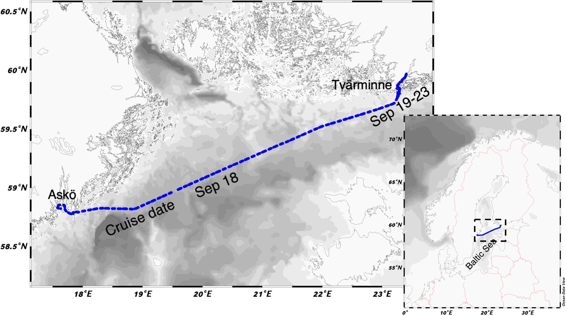
Figure 1. Cruise track.

Statistical Evaluation of Long-Term Temperature Records

The long-term temperature record from the TZS coastal monitoring site (lat: 59.85548N, lon: 23.26033E) covers August 1926 to December 2018. A moving average was adopted to smooth the short-term fluctuations in the temperature data by taking the average value of a 1-year length and shifting forward, i.e., for each average annual value calculation, the first number of the 1-year data series was excluded and the next value was included. Note that the time interval of each temperature record varied slightly, from 10 days in the years before 1997 down to 4–7 days after 1998 and finally daily records in 2018. Thus, the 1-year length used in this study is fixed from a day in a year to the same day in the year after regardless of the time interval between two specific temperature records.

Continuous CO₂ and CH₄ Measurements in Surface Water and Atmosphere

The partial pressures of atmospheric and dissolved CO₂ and CH₄ were measured using the Water Equilibration Gas Analyzer System (WEGAS) coupled to cavity ring-down spectrometer (CRDS). This system consists of three major components: (i) a water handling system comprised of a showerhead equilibrator (1 L headspace volume) fed by the seawater intake, an E&H electrode probe and a thermosalinograph (Seabird TSG 45); (ii) a gas handling system with circulation pumps for the showerhead and ambient air from the bow of the ship; and (iii) CRDS gas analyzers for CO₂ and CH₄ concentrations (model G2131-i, Picarro Inc.); and A detailed description of the WEGAS systems and its performance can be found in the Supplementary Material.

Measurements of surface water CO₂ and CH₄ concentrations were performed using the seawater intake located just below the sea surface. Water was pumped through spray nozzles into the open headspace equilibrator at ∼4.5 L min^–1. By creating a fine spray of droplets, the exchange surface between showerhead and water was maximized and an optimal equilibration is achieved. The ambient pressure was maintained through a ambient air-fed vent flow that was monitored continuously during the measurements. The gas equilibrated in the showerhead was measured using the CRDS analyzer. For the standard CO₂ and CH₄ analysis routine, ambient air is measured for 8 min followed by the gas measurements in the showerhead of the equilibrator for 12 min, i.e., one complete analysis cycle is 20 min. Cycles are performed continuously during the cruise including the station time when RV Electra is not steaming.

Continuous CO₂ and CH₄ measurements in both ambient air and surface water were conducted during September 18–23, 2018; in total, 80,393 data points for both CO₂ and CH₄ in air and water were recorded. The recorded data were filtered by removing data taken during the transition period between ambient air and water measurements (see detailed description in Supplementary Material) and collected during improper functioning of WEGAS (e.g., low water flow, exceptional values due to air contamination by the ship) and thereafter the data were also corrected for the vent flow to the equilibrator that was induced while WEGAS was running. Any remaining data with CO₂ concentrations above 450 ppm were also removed. After filtering, atmospheric CO₂ averaged 401.3 ± 2.08 ppm (2σ). As a result of spatial normalization and excluding data that could have been contaminated by the ship, here we present 15,733 data points for both air and water concentrations.

For reporting the CO₂ content in water, the ppm value obtained by the cavity ring down spectrometer (CRDS) were converted to pressure units (pCO2 in μatm). We assumed ambient atmospheric pressure because water was taken at depth of around half a meter below the surface and the pressure in the showerhead is equal to ambient air as achieved by the vent flow taken at the bow of the ship.

For reporting the CH₄ concentrations in water, the ppm value obtained by CRDS were converted to molar units (i.e., nmol/L) by Henry’s law (Equation 1), because the achieved equilibration means that the gas content in the showerhead is equivalent to that in the water phase, i.e., CH₄ measured by CRDS is considered as the real-time concentration of CH₄ in water. This makes Henry’s law applicable for dealing with gas/liquid equilibria and the Henry’s constant for molar concentration and partial pressure conversion is chosen in this case. As the showerhead in the equilibrator is maintained at ambient pressure and the water temperature is measured by thermosalinograph right before the water reaches the equilibrator, Henry’s law constant is corrected for each calculation by the measured temperature at atmospheric pressure.

$$C=p\times K_{\text{H}}(1)$$

where C is the concentration of CH₄ (mol/L), p is the partial pressure in unit of atm (1 atm = 10⁶ ppm) of CH₄. K_H is the Henry’s law constant that is dependent on temperature and is corrected in this study following the van ’t Hoff equation (Sander, 2015):

$$K_{\text{H}}=K_{\text{H}}^{{}^{*}}\times \text{exp}[\frac{-{\mathrm{\Delta }}_{\text{sol}}H}{R}\times (\frac{1}{T}-\frac{1}{T^{{}^{*}}})](2)$$

Where $K_{\text{H}}^{{}^{*}}$ is the Henry’s law constant at the reference temperature, 298 K, T^* is the reference temperature, 298 K and T is the measured temperature in water (K). The temperature dependence of the equilibrium constant, $\frac{-{\mathrm{\Delta }}_{\text{sol}}H}{R}$ does not change much with temperature and is tabulated (Sander, 2015). K_H also varies with pressure, but in this study, pressure was assumed to be atmospheric pressure because water was taken at depth of around half a meter.

In the Baltic Sea both CO₂ and CH₄ concentrations span an order of magnitude and the highest concentrations reported are >2500 μatm of CO₂ (Fransner et al., 2019) and >1200 nM of CH₄ (Jakobs et al., 2014).

Calculations of Sea-Air Gas Fluxes

The sea-air flux (F) of CO₂ and CH₄ is commonly expressed by the following equation (Liss and Slater, 1974):

$$F=k\times \left(C_{\text{sea}}-C_{\text{air}}\right)(3)$$

where k is the gas transfer velocity and C_sea and C_air are concentrations of gases in the sea and the overlying air, respectively. This is also frequently written as Equation 4

$$F=k\times K_0\times \left(p_{\text{sea}}-p_{\text{air}}\right)(4)$$

where K₀ is the solubility of CO₂ or CH₄, p_sea and p_air are the measured partial pressures of the gases in equilibrium with surface water and in the air, respectively. k is the gas transfer velocity that has been optimized as Equation 5 (Wanninkhof, 2014):

$$k=0.251\times U^2\times {\left(\frac{Sc}{660}\right)}^{-0.5}(5)$$

where U is wind speed (m/s) and Sc is the Schmidt number, which is highly dependent on temperature and gas. Sc in our calculations was corrected for the corresponding temperature that was measured simultaneously with partial pressures of CH₄ and CO₂ (pCH₄ and pCO₂).

Combining Equations 3, 4 and 5, the flux of CO₂ and CH₄ in this study is finally calculated as Equation 6:

$$F=0.251\times U^2\times {\left(\frac{Sc}{660}\right)}^{-0.5}\times K_0\times \left(p_{\text{sea}}-p_{\text{air}}\right)(6)$$

Regional Meteorological and Oceanographic Data

Surface water temperature data observation in the open Northern Baltic Proper from the automatic buoy Huvudskär (lat: 58.9333 N, lon: 19.1667 E; 100 m water depth) were retrieved from the Swedish Hydrological and Meteorological Service². Wind data observation from the Raasepori Jussarö (lat: 59.82076N, lon: 23.57309E) weather station and wave height observations from the buoy Raassepori Hästö Busö (lat: 59.82583N, lon: 23.30783E), which are located some 15 km and 5 km from the TZS, respectively, were retrieved from Finnish Meteorological Institute³.

Box Model Approach to Address Sources and Sinks of CO₂ and CH₄

Using the surface CO₂ and CH₄ concentration in inshore and offshore surface waters and sea-air flux data and the information about the deepening of the upper mixed surface layer after the storm event, we can construct a budget evaluating the sources and sinks of CO₂ and CH₄ (Figure 2). The conservation of mass for the surface layer under the assumptions mentioned is:

$${\text{h}}_{\text{after}}C{O}_{2after}-{\text{h}}_{\text{before}}C{O}_{2before}=C{O}_{2offshore}(h_{\text{after}}-h_{\text{before}})-F_{{\mathrm{CO}}_2}\mathrm{\Delta }t+I_{{\mathrm{CO}}_2}\mathrm{\Delta }t(7)$$

$${\text{h}}_{\text{after}}C{H}_{4after}-{\text{h}}_{\text{before}}C{H}_{4before}=C{H}_{4offshore}(h_{\text{after}}-h_{\text{before}})-F_{{\mathrm{CH}}_4}\mathrm{\Delta }t+I_{{\mathrm{CH}}_4}\mathrm{\Delta }t(8)$$

FIGURE 2

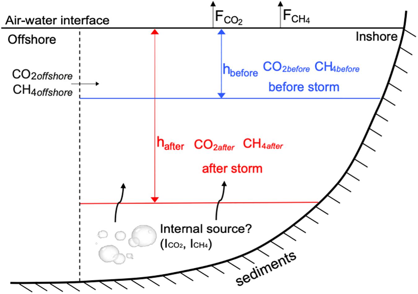
Figure 2. Scheme over the budget approach evaluating the internal sources and sinks of CO₂ and CH₄ in TZS coastal waters.

Where h is the mixed layer depth before and after the storm, respectively, F atmospheric flux and I an internal source term. The source water for the advection term, i.e., CO_2offshore and CH_4offshore are assumed to have properties close to what was observed offshore on September 19 and 20.

Continuous Measurements of Gas Flares and Bubbles

The acoustic water column data presented here were continuously collected with a Simrad EK80 wideband split-beam scientific echo sounder with a center frequency at 70 kHz that was installed on RV Electra. The vertical range resolution is approximately 2 cm and the ping rate was about 2.5 Hz. The sonar produces a linear frequency modulated acoustic signal which provides improved signal-to-noise ratio and a higher vertical range resolution compared to similar narrow-band systems (Stanton and Chu, 2008). The dataset collected with the EK80 was match filtered with an ideal replica signal using a MATLAB software package version R2017a provided by the system manufacturer, Kongsberg Maritime (Lars Anderson, personal communication). Position and altitude information were provided to the sonar by a Seapath 330 + motion sensor. Ranges from the transducer were calculated using the cumulative travel times through sound speed profile layers based on the nearest (in time) CTD profile (SEA-Bird SBE 911 plus), following the approach by Stranne et al. (2017).

Results

Temperature Records in the Open Northern Baltic Proper and in the Finnish Coastal Waters Near Tvärminne

Temperatures of up to 23.04°C (daily mean) were recorded in the upper surface layer in the open Northern Baltic Proper on 6 August at the autonomous measuring stations (Figure 3A). A similar picture appears when evaluating the coastal monitoring stations near TZS. Since 2017, water temperatures have been continuously recorded using in situ instrumentation, allowing us to follow the effects of the summer 2018 heat wave in even greater detail. The highest bottom-water temperatures (32 m depth) of 20.53°C were recorded on 30 July at this coastal monitoring station (Figure 3B) and these are the highest temperatures ever recorded at this depth over the past 93 years. A second warming event in bottom waters above the sediments was recorded in early September 2018 just before our sampling campaign with temperatures reaching nearly 17°C (Figure 2B). The record-high bottom temperatures measured in the TZS area in 2018 follow an increasing trend observed over the past century until today. In Figure 3C, the long-term temperature record (moving average) between 1926 and 2018 is presented showing a mean water temperature of 4°C above the sediments between the 1920s and the 1980s. Thereafter, we see a dramatic increase in bottom-water temperatures starting in the 1990s to about 6°C in the 2010s.

FIGURE 3

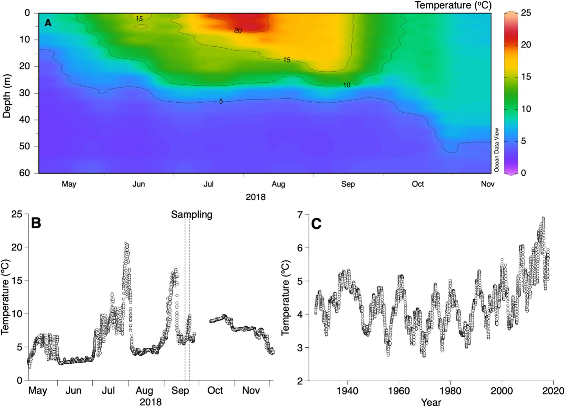
Figure 3. Temperature records from (A) open Baltic Sea (vertical water column profile) during the heat wave in 2018 (May–November; Huvudskär, lat: 58.9333, lon: 19.1667; 100 m water depth; daily average), (B) bottom waters (31 m water depth) at the TZS coastal monitoring site during the heat wave in 2018 (May–November; Storfjärden, lat: 59.85548, lon: 23.26033; hourly measurements) and (C) bottom waters (31 m water depth) at the TZS coastal monitoring site (long-term temperature data 1926–2018; 1-year moving average).

Spatial CO₂ and CH₄ Patterns in Open vs. Coastal Areas of the Baltic Sea

Surface-water temperatures were between 14 and 18°C throughout the transect (Figure 4A) which is somewhat cooler than at the peak of the heat wave during July/August, when temperatures of up to 23°C were recorded in the surface layer (Figure 3A). Both pCO₂ and CH₄ concentrations were closer to equilibrium with the atmosphere in the central basin of the Northern Baltic Proper, but they were elevated in coastal areas (Figures 4C,D). However, off the Swedish coast at 70–100 m water depth, we encountered an upwelling event indicated by low temperatures and high salinity at the water surface (Figures 4A,B) and with elevated pCO₂ of up to >800 μatm (Figure 4C). CH₄ showed only moderately elevated concentrations of 12 nmol/L (Figure 4D). Toward the Finnish coast, both CO₂ and CH₄ gradually increased to concentrations of ∼700 μatm for CO₂ and over 30 nmol/L for CH₄. Partial pressure and concentration vs. seafloor depth plots reveal that in coastal areas, with water depths <40 m, both CO₂ and CH₄ (Figures 5A,B) show more elevated pCO₂ and CH₄ concentrations in the upper mixed layer compared to the open Northern Baltic Proper.

FIGURE 4

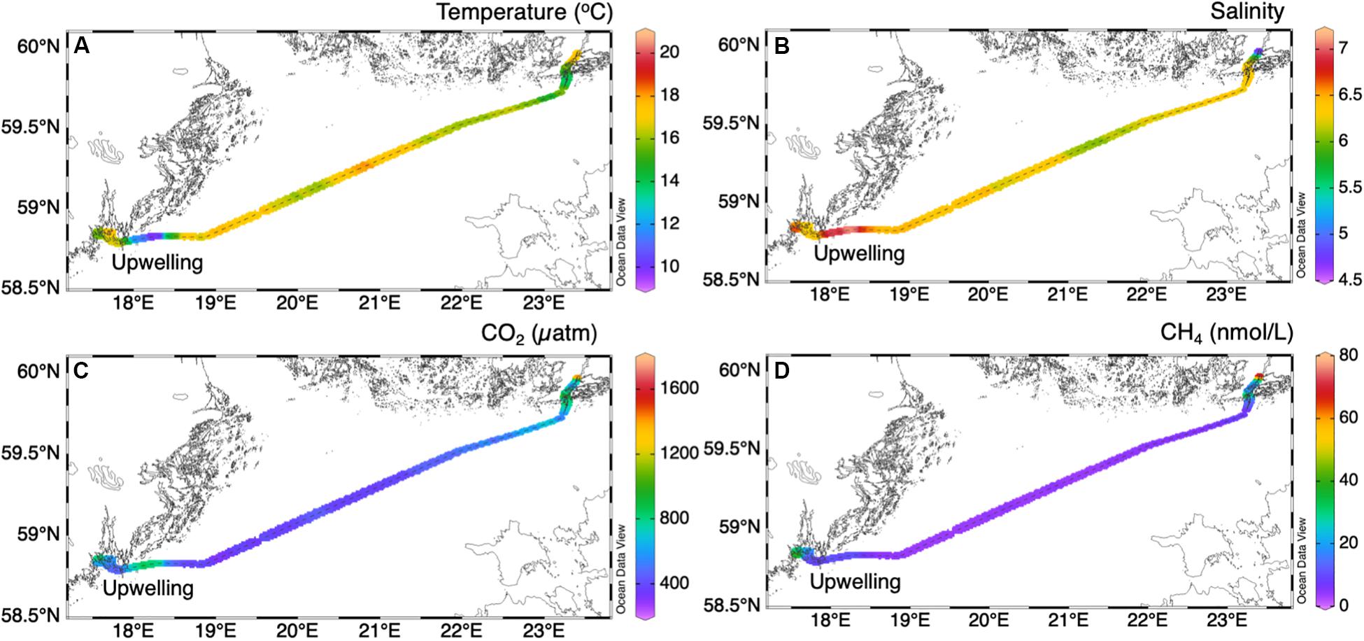
Figure 4. Cross section from Askö to Tvärminne of (A) temperature, (B) salinity, (C) pCO₂ (μatm) and (D) CH₄ concentrations (nmol/L) in surface waters.

FIGURE 5

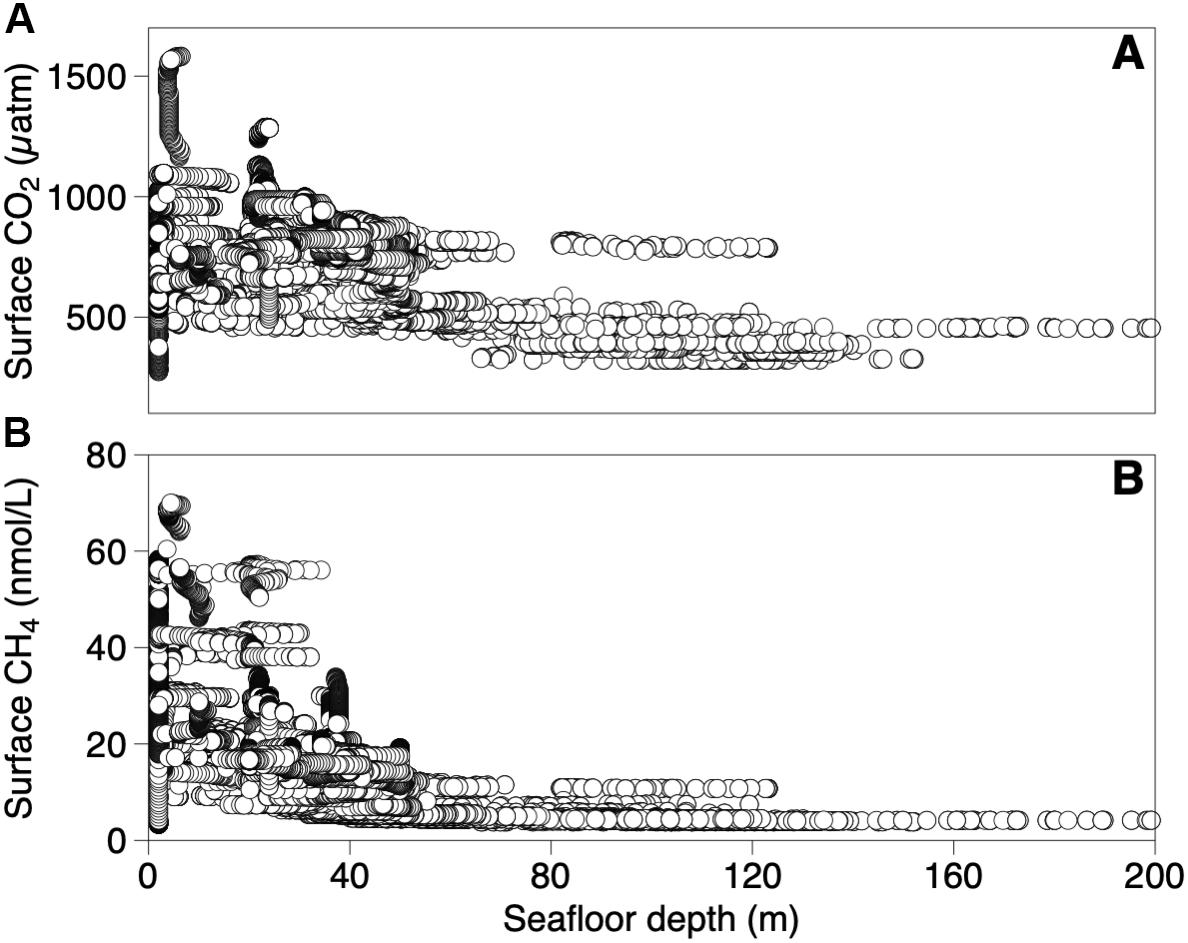
Figure 5. (A) pCO₂ (μatm) and (B) CH₄ concentration (nmol/L) in the surface waters vs. seafloor depth along the cross section from Askö to Tvärminne.

At the easternmost end of the transect, we investigated parts of Finnish Archipelago Sea near the TZS in more detail between September 19–23, 2018. pCO₂ and CH₄ concentrations followed a salinity gradient with higher values toward the freshwater end-member (Figure 6) that is formed by the small river Karjaanjoki (runoff 0.59 km³ y^–1, Räike et al., 2012) that runs into the Pojo Bay and further into the Storfjärden Bay (black dashed box in Figure 8A). The highest pCO₂ (1583 μatm) was measured at the northernmost part of the Storfjärden where salinities were <5 psu. A similar pattern was recorded for CH₄, which reached its highest concentration of 70 nmol/L a bit south from the position where CO₂ peak concentrations were found. An interesting pattern appeared when plotting pCO₂ and CH₄ concentrations against seafloor depth (Figure 7). pCO₂ in surface water were lowest at the shallowest seafloor depth and continuously increased from 751 μatm at <5 m seafloor depth to 1020 μatm at 20–25 m seafloor depth (Figure 7A). In contrast, the high CH₄ concentration of 44 nmol/L (median) was recorded at the lowest seafloor depth, while concentrations ranged between 24 and 40 nmol/L at deeper depths between 5 and 25 m (Figure 7B). Note, that all median pCO₂ values and CH₄ concentrations were calculated before the wind event described in the next section.

FIGURE 6

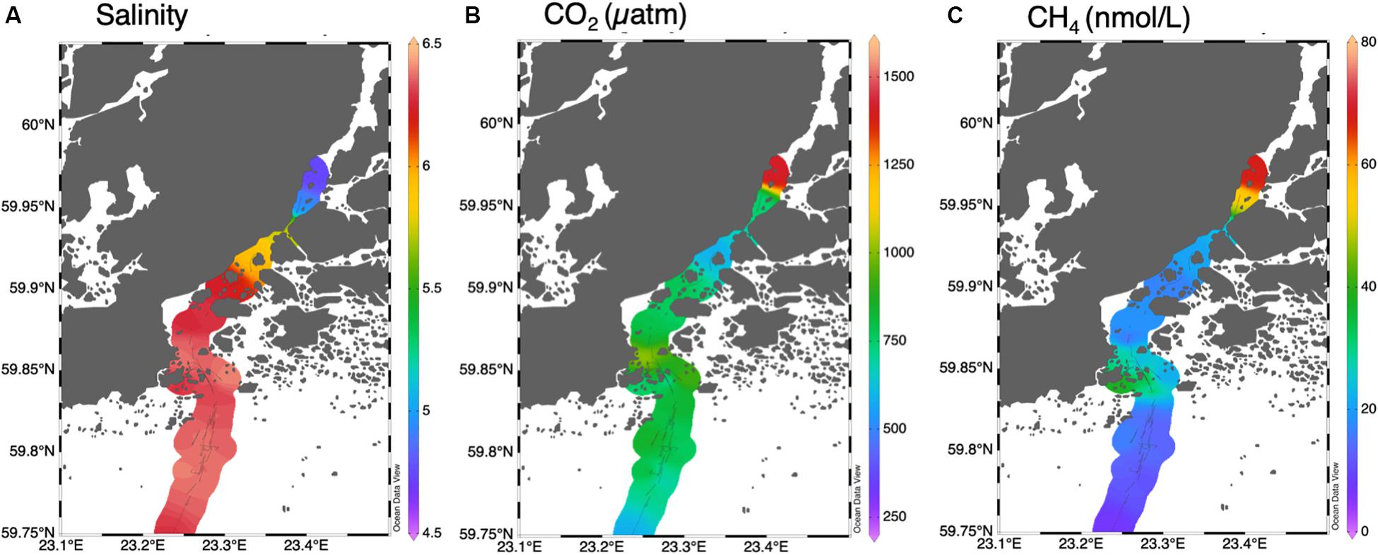
Figure 6. Surface distribution of (A) salinity, (B) pCO₂ (μatm), and (C) CH₄ concentrations (nmol/L) within the TZS coastal waters; the black dots indicate daily cruise tracks within the area.

FIGURE 7

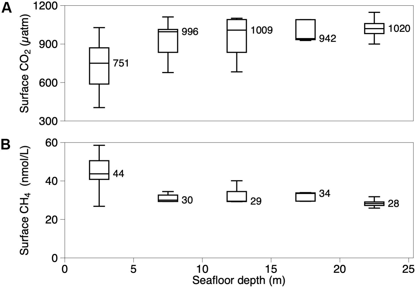
Figure 7. (A) pCO₂ (μatm) and (B) CH₄ concentrations (nmol/L) as grouped by seafloor depth within TZS coastal waters before the storm event.

FIGURE 8

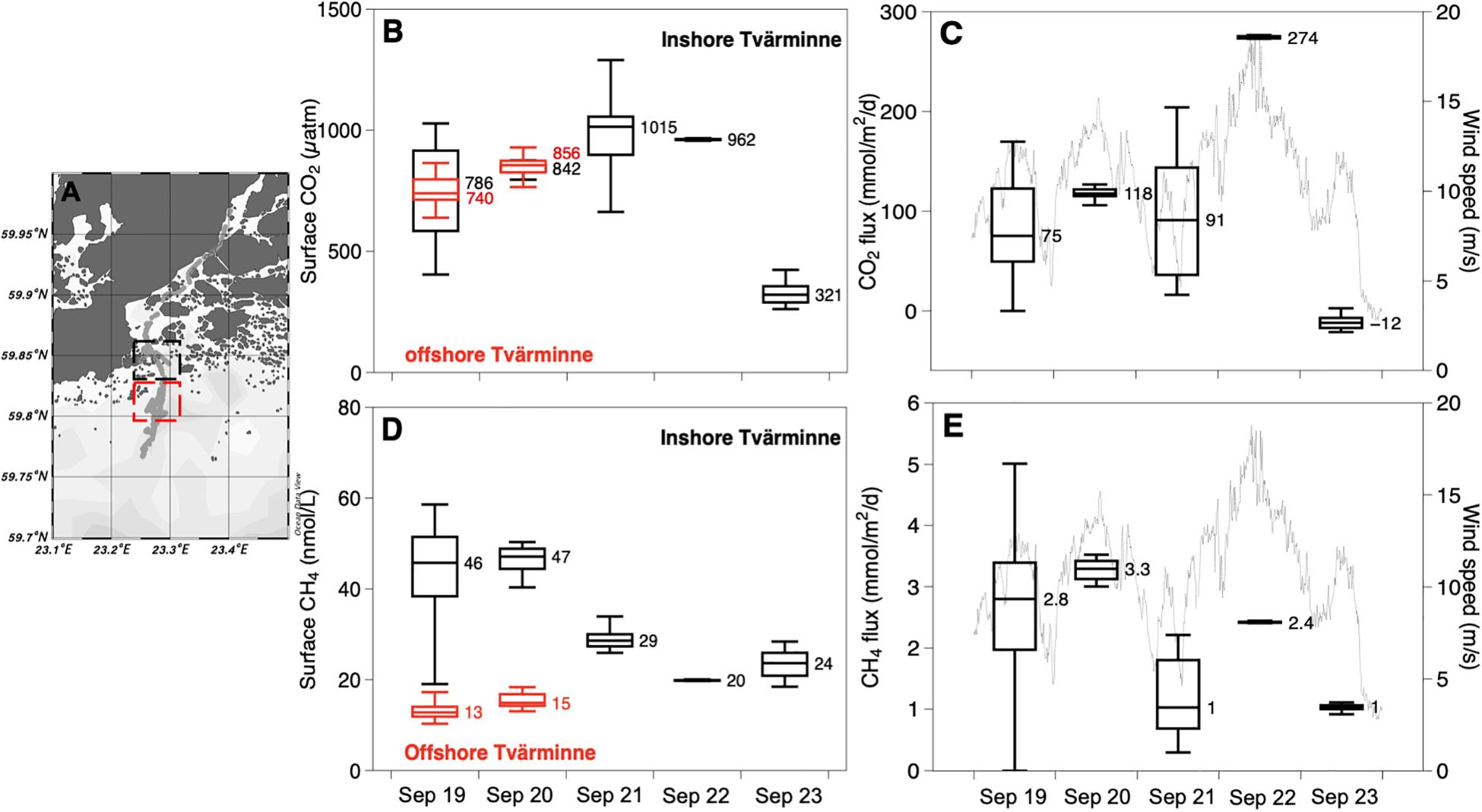
Figure 8. Temporal variations in the surface waters in the inshore (black dashed square in A) and offshore (red dashed square in A) TZS coastal area (A) of (B) pCO₂ (μatm), (C) CO₂ flux (mmol/m²/d), (D) CH₄ concentration (nmol/L) and (E) CH₄ flux (mmol/m²/d) including wind speed between September 19 and 23.

Wind-Induced Changes in CO₂ and CH₄ Water Column Inventories and Inferred CO₂ and CH₄ Source and Sink Terms in Coastal Waters

Figures 8B,D show the temporal development of pCO₂ and CH₄ concentrations inshore and offshore the TZS coastal area. Elevated pCO₂ of some 800 μatm were recorded by the WEGAS system on September 19 and 20 within the inshore waters (indicated with the black dashed box in Figure 8A) and the offshore pCO₂ (indicated with the red dashed box in Figure 8A) were also at the same elevated range as the inshore concentrations (median of 740–856 μatm; Figure 8B). During sampling on September 21, the wind gradually increased from 5 m sec^–1 to some 10 m sec^–1 and pCO₂ in the inshore waters increased to 1,015 μatm, although this increase is not significant when taking the variability of the measurements in the inshore waters that day (between 700 and 1 300 μatm; Figure 8B) into account. Wave height increased simultaneously from 0.6 to 1.6 m. Wind speeds peaked at 20 m sec^–1 during September 22 and decreased again down to 3 m sec^–1 during the evening hours of September 23 (Figure 8C). During the same time peak wave height of 1.9 m was recorded at the monitoring buoy near TZS, which decreased to 0.5 m. Thus, during the entire period between September 19–23 the average wind was between 8 and 10 m sec^–1 (0.5–0.8 m wave height), disrupted by the peak wind event on September 22 with wave heights of up to 1.9 m. CO₂ sea-air fluxes were greatest during this peak wind event with 274 mmol m^–2 d^–1 (Figure 8C), whereas at the end of the wind event, CO₂ was undersaturated in the upper surface layer and even negative sea-air fluxes were calculated. However, during the entire wind event, the pCO₂ decreased sharply from a 2–3 times oversaturation (median of 1015 μatm) to a slight undersaturation (median of 321 μatm recorded at September 23). Thus, the wind event rather effectively depleted the water column with respect to pCO₂.

In contrast to the expected depletion of CO₂ from oversaturation caused by the wind event, CH₄ remained oversaturated before, during, and also after the wind event. Elevated CH₄ concentrations of 46 – 47 nmol/L (median; Figure 8D) were recorded by the WEGAS system on September 19 and 20 within the inshore waters, whereas for the offshore waters CH₄ concentrations were also supersaturated, but less so, with median concentrations between 13 and 15 nmol/L. During and after the wind event during September 22, CH₄ concentrations decreased in the inshore waters to a median value of 20–24 nmol/L, however, remained oversaturated by 5–8 times. Accordingly, the CH₄ sea-air flux calculations (Figure 8E) revealed the highest CH₄ average fluxes between 2.8 – 3.3 mmol m^–2 d^–1 before the wind event and lower, but still elevated, fluxes between 1.0 – 2.4 mmol m^–2 d^–1 during and after the wind event.

Although wind is directly related to the gas transfer velocity (k) in Equation 3, wind speed could only partly explain the variation in both CO₂ and CH₄ fluxes. However, the highest CH₄ fluxes were observed at relatively low winds (12 m sec^–1), whereas the highest CO₂ fluxes were observed at peak wind speeds (Figures 8C,E). Accordingly, the CO₂ and CH₄ fluxes show positive relationship (not shown), however, the highest CH₄ fluxes were recorded at very low CO₂ flux regimes, which indicates that CH₄ flux events are decoupled from CO₂ flux events during low wind regimes (9–12 m sec^–1).

As indicated in Figures 8C,E, the wind increased significantly after September 21 from less than 10 to nearly 20 m sec^–1. Simultaneously, CTD data collected between September 21 (10:25 UTC) and September 23 (14:00 UTC) show a deepening of the surface mixed layer after the wind event (Figure 9). Note that the temperature (Figure 9B) before and after the wind event (September 22) remained more or less constant at 11°C and that salinity (Figure 9C) decreased only slightly from 6.5 to 6.4 psu, whereas the upper mixed layer depth increased from roughly 10–25 m water depth. Thus, the surface mixed layer increased over these 2 days in depth from about 10 m to nearly 25 m and this was mainly caused by a downwelling event triggered by south-southeasterly winds pressing water masses into the Finnish inner coastal waters rather than by vertical mixing. Thereafter, the mixed layer depth remained at the same depth for the remainder of the cruise.

FIGURE 9

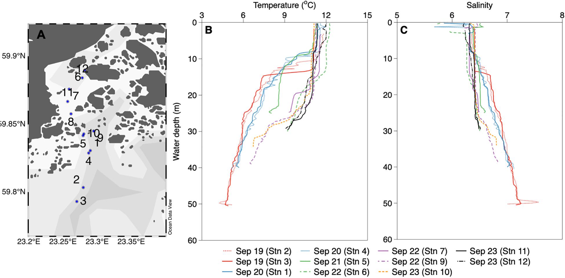
Figure 9. Ventilation of the upper mixed layer in TZS coastal waters (A) by the storm event as demonstrated by vertical temperature (B) and salinity (C) profiles taken between 19 and 23 September 2018; position of individual CTD casts are indicated by station numbers in (A).

The concentrations, mixed layer depths, and atmospheric fluxes used to estimate the internal sink/source terms are given in Table 1. We assume that the transition occurs during 24 h corresponding to approximately the time of the storm event and the interval between the two CTD profiles mentioned above. The results of the budget calculation indicate a net sink of CO₂ in the water column, however, the sink could be somewhat overestimated because the offshore concentrations decreased due to the massive outgassing. Further, the budget indicates a CH₄ source of about 2.5 mmol m^–2 d^–1 from below the mixed surface layer.

TABLE 1

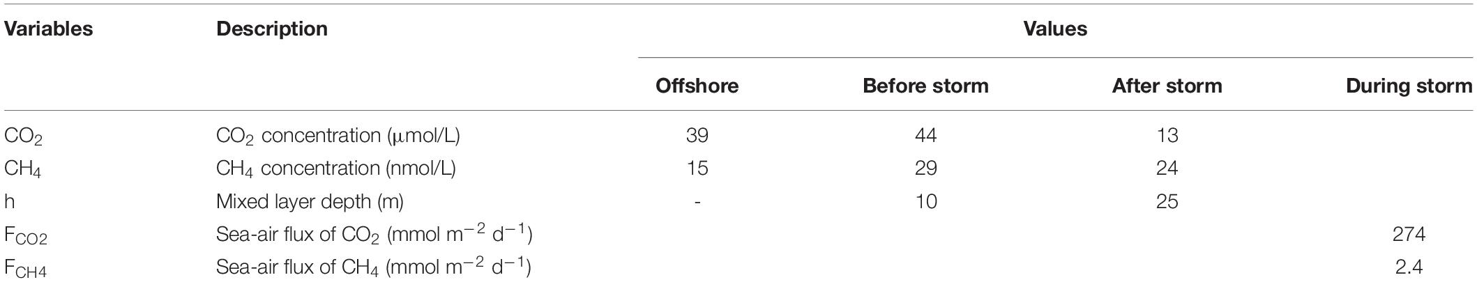
Table 1. Concentrations, fluxes and mixed layer depths used in the box model calculations of CO₂ and CH₄ sources and sinks in TZS coastal waters during the storm event 21–23 September 2018.

A possible explanation for the deviating patterns of CO₂ vs. CH₄ fluxes can be found in the geophysical variables investigated and continuously recorded during the cruise. The acoustic mid-water mapping revealed vigorous and widespread gas flares from the sediments in the Finnish coastal waters as exemplified in Figure 10 where some 10–15 major flares and numerous trains of individual bubbles are visible along a 3 km transect, indicating intense bubble formation and ebullition at the sea floor. Further, gas bubbles are visible throughout the entire water column up to the water surface, penetrating into the mixed surface layer that was situated at around 10–15 m water depth (based on CTD data, Figure 9). The mixed layer is also discernable in the echogram, although vaguer than observations made in Arctic Ocean coastal waters (Stranne et al., 2017).

FIGURE 10

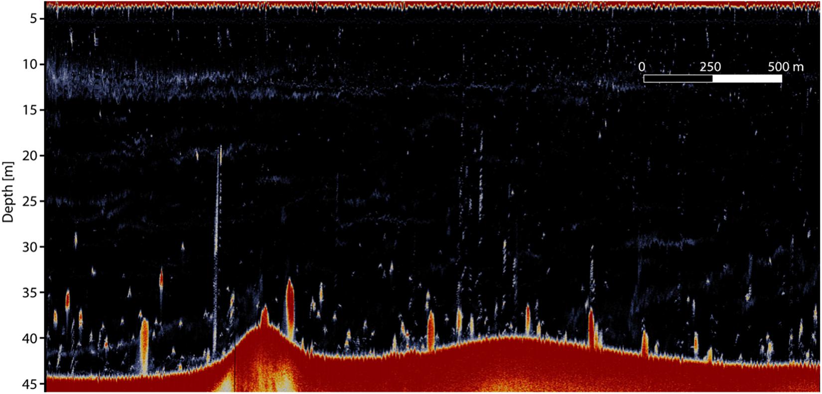
Figure 10. EK80 echogram showing acoustic anomalies associated with gas seeps from the bottom sediments in TZS coastal area (black dashed square in Figure 8A), following the cruise track from left to right and with color indicating the acoustic target strength (black is <–80 dB and red is >–60 dB). Compass coordinates for the beginning/end of the echogram (23° 17.4′ E, 59° 49.8′ N)/(23° 16.4′ E, 59° 49.0′ N).

Discussion

On a global scale, lakes and rivers are significant sources for CO₂ and CH₄, and their fluxes are relatively well constrained compared to the evaluation of sinks and sources in the global coastal ocean. CO₂ emissions from lakes and reservoirs are estimated to be 0.32 Pg C yr^–1 and from rivers and streams to be 1.8 Pg C yr^–1 (Raymond et al., 2013), whereas CH₄ emissions from inland waters are estimated to be 77 Tg C yr^–1 (Bastviken et al., 2011). Upscaling exercises using a typology approach including four estuarine types and different types of continental shelves along three climatic zones estimates global CO₂ emissions to be 0.27 Pg C yr^–1, whereas global CH₄ emissions from estuaries to be 5.0 Tg C yr^–1 (Laruelle et al., 2010; Borges and Abril, 2012). However, Laruelle et al. (2010) conclude that “the largest uncertainty of scaling approaches remains in the variability of CO₂ data to describe the spatial variability, and to capture relevant scales of variability.” Note that the global estimates of coastal gas emissions are biased toward the many investigations focusing on estuaries, lagoons, salt marches, and tidal flats (Borges and Abril, 2012), whereas studies capturing shorelines that are less affected by river inputs are less studied. Further, CH₄ emissions in coastal areas are clearly coupled to temperature (Borges et al., 2016; Sawicka and Brüchert, 2017) and the highest rates of change are to be expected in organic-rich shallower parts affected by warming water bodies overlaying marine sediments. In fact, experimental studies show that a temperature increase of only 2°C can increase anaerobic organic matter degradation by 40% in marine sediments (Roussel et al., 2015). We clearly demonstrate in this study that the temperature increases in Finnish coastal waters correspond to such a 2°C rise during the last 3 decades. Bottom waters and surface sediments in this sub-arctic setting experience peak temperatures of over 20°C coinciding with elevated CO₂ and CH₄ concentrations and fluxes that are comparable to the more frequently investigated terrestrial hot spots for CO₂ and CH₄ emissions, such as arctic lakes, wetlands and thawing permafrost areas.

We suggest that the sea-air CH₄ flux is likely dominated by frequent bubbling from sediments, which we observed even during low winds, when CO₂ fluxes were at their minimum, high CH₄ fluxes occurred, knowing that this notion lacks a quantitative approach that has to be developed in the future by new ways of interpreting geophysical data of the water column. However, we have shown that surface CH₄ concentrations were highest at the shallowest seafloor depth (Figure 7) indicating that the proximity to the sediments and gas flares as well as the short residence times that prevent full CH₄-oxidation in the water column as observed in the deep open ocean (Reeburgh, 2007). In contrast, CO₂ in surface water shows a positive relationship with seafloor depths, indicating that respiration of autochthonous and allochthonous organic carbon in the water column is the predominant source for CO₂ even in shallow coastal systems. This has bearing for the understanding and future model parametrizations especially of CH₄ fluxes in arctic and subarctic shelf systems, i.e., a comprehensive understanding of spatial and seasonal CH₄ accumulation and flare distribution in sediments as stimulated by heat waves is needed to quantify CH₄ fluxes from shallow coastal waters. Acoustic methods directly addressing bubble-mediated methane flux are becoming more available (Weidner et al., 2019) and similar studies using mid-water sonar systems near Spitzbergen have shown that CH₄ partly originating from ebullition and transformed into the dissolved pool during upward transport is efficiently trapped below the halocline at some 200 m water depth for at least part of the year, which prevents outgassing to the atmosphere (Gentz et al., 2014). This is corroborated by our findings in the deeper stratified Northern Baltic Proper where even a strong upwelling event led to strong outgassing of CO₂ (Figure 4C), but only moderate increased CH₄ concentrations were observed (Figure 4D). Recent findings suggest that methanogenic Archaea in zooplankton guts significantly contributes to the CH₄ supersaturation in the upper surface layer of the Baltic Sea (Schmale et al., 2018), i.e., the role of bubble-mediated CH₄ transport in the central parts of Baltic appear less likely. In shallow coastal areas the role of such pelagic sources may presumably be less important, because the zooplankton biomass is simply limited by the lower volume of water, but this cannot be ruled out.

We observed a pronounced pycnocline also in the coastal waters around TZS (Figure 9), but in this shallow coastal setting we could observe bubbles rising from the seafloor and throughout the entire water column and penetrating the pycnocline (Figure 10). Note that the WEGAS system is capturing both diffusive and bubble flux collected by the sea water intake. We do not know whether a CH₄ reservoir has accumulated below the pycnocline in the Finnish coastal waters and thereby contributing to the elevated CH₄ concentration in the water column and significant sea-air fluxes. However, gas bubbles can only survive a certain rise height of some 100 m in the water column before they are depleted in CH₄ (McGinnis et al., 2006). Once CH₄ is dissolved, it is prone to oxidation before reaching the atmosphere and here vertical density gradients such as pycnoclines form a barrier for dissolved CH₄. This barrier to CH₄ transport from the seafloor to the atmosphere does not work in shallow coastal systems where ebullition from the seafloor can reach the atmosphere directly and our investigations show intensive bubble mediated transport between the sediments and the atmosphere down to 45 m water depth (Figure 10). Future investigations will show whether CH₄ concentrations in the bubbles do decrease with increasing water column travel time, i.e., whether these bubbles still contain significant amounts of CH₄ when reaching the sea-air interface. Further, it appears highly likely that the gas bubbles are of biogenic origin, because we found an inverse pattern, though not statistically significant, between CH₄ concentrations and seafloor depth and/or proximity to the shore (Figures 6, 7) – a coastal effect. Eutrophication, high productivity and organic matter from runoff leads to accumulation of sediments with thick sequences of organic mud nearshore the TZS coastal area (Kauppi et al., 2018), which in turn leads to methane production and seepage. These patterns wouldn’t appear when the bubbles were of thermogenic origin, i.e., from petrogenic deposits that may occur in folds that should be more randomly distributed.

A striking result of this study is that CH₄, which has a lower solubility compared to CO₂, never equilibrated with the atmosphere, whereas simultaneously the slower reacting gas (CO₂) with a higher solubility was depleted within a few hours after the wind event. Our box model approach inferred a source term for CH₄ – that might originate directly from sediment flares, or a diffusive flux from the sediments and a theoretical water column reservoir – that is significant (2.5 mmol m^–2 d^–1 or 30 mg C m^–2 d^–1). A comparable benthic study from the nearshore shallow coastal areas along the Swedish coast (Sawicka and Brüchert, 2017) reported nearshore sediment-water fluxes between 0.1 and 2.6 mmolm^–2d^–1. Our reported rate is at the high end, indicating that the heat wave played an important role in a massive flux event of CH₄, although we have to bear in mind that the benthic sediment fluxes and fluxes from a potential reservoir in the water column cannot be disentangled from our CH₄ supply estimates. Although we do not have any quantitative measurements, the observed extensive occurrence of gas flares and bubbles point toward a significant contribution from the sediments. A comparable study addressing sea-air fluxes in the North Sea (Borges et al., 2018) report elevated fluxes between 28 and 126 mmol m^–2 per year. Our observed accumulated flux for the 5-day period at the end of the heat wave was 11 mmol m^–2 (averagely 2.2 mmol m^–2 d^–1), which is similar to CH₄ emissions observed in thermokarst lakes in subarctic areas (Matveev et al., 2016). This result supplies further evidence that heat waves trigger massive CH₄ fluxes to the atmosphere from nearshore sites.

The sea-air CO₂ exchange of 75–274 mmol m^–2 d^–1 or 0.9–3.3 g C m^–2 d^–1 also indicates extreme outgassing during the end of the heat wave and can be compared with recent model studies indicating outgassing of up to 60 g C m^–2 yr^–1 in the nearshore areas of the northern Baltic Sea (Fransner et al., 2019). It is of course difficult to compare simulated annual rates with our measurements that were taken over a few days but it is, nevertheless, striking that the daily sea-air exchange rates of CO₂ presented here are one order of magnitude higher than the simulated ones. It could be that the effects of heat waves followed by increasing autumn winds for the outgassing of CO₂ haven’t been considered, i.e., our 5-day estimated sea-air exchange of 6.5 g C m^–2 is already 10% of the highest simulated annual values reproducing the spatial hot spots near the coast. The model has been calibrated/validated with ferry-box observations and clearly indicates the classical CO₂ accumulation of up to 2500 μatm under the ice and values close to equilibrium in ice-out situations. However, this study demonstrates that heat waves produce similar accumulations of CO₂ in the water column and the outgassing events can be as significant as ice-out situations that have been described also for other high latitude coastal systems, such as the East Siberia Sea (Thornton et al., 2016; Humborg et al., 2017).

Conclusion

In the past decade, continuously recording CO₂ and CH₄ instruments have become state-of-the-art equipment on large research vessels and on commercial ships which run ferry-box solutions. Thus, we have a fairly good understanding of CO₂ and CH₄ exchange processes in open waters of the Baltic Sea, the open Atlantic, or even in remote areas as the Siberian Sea (Körtzinger et al., 1996; Gülzow et al., 2011; Schneider et al., 2014; Thornton et al., 2016; Humborg et al., 2017). Even sediment-water exchange of CH₄ is investigated by automated lander techniques, and many of these studies focus on deeper sites (Boetius and Wenzhöfer, 2013). For the Baltic Sea and the North Sea, there are only a few datasets on nearshore shallow area emissions available and this situation may be representative for many shallow coastal systems that make up half of the Baltic Sea or a third of the global continental shelfs. In this study we show that these nearshore coastal systems are CO₂ and CH₄ emission hotspots and fluxes are comparable to terrestrial hot spot in Arctic lakes (Huttunen et al., 2006; Repo et al., 2007; Juutinen et al., 2009; Wik et al., 2013) and that shallow coastal systems are highly responsive to ongoing changes in temperature. Coastal seascapes constitute a mosaic of heterogeneous environments and habitats, and sediment-water interactions become more pertinent compared to the well-studied open coastal and ocean waters. For shallow coastal waters, the non-invasive and continuous instruments that record sediment and water column gas inventories and fluxes are still not sufficiently used and must be deployed on small research vessels that can reach the shallowest sites, which often host complex habitats such as algal belts, mussel beds, or seaweeds. The combination of the automated continuous CO₂- and CH₄-measurement devices and lander techniques, together with modern geophysics as mid-water sonar, multibeam or sub-bottom profilers, will allow identifying gas accumulations, pock marks, as well as flares and bubbles. As a result, we hypothesize that the sediment accumulation and event driven high gas emissions from nearshore shallow sediments is a major carbon capacitor in coastal areas that is not accounted for by the classical invasive core-incubation methods (Reeburgh, 1968) or by lander techniques (Boetius and Wenzhöfer, 2013) that still govern our view and process understanding of sediment-water CH₄ fluxes, and that these event-driven massive fluxes will increase with rising temperatures.

Data Availability

All data necessary to evaluate and build upon the work in this manuscript can be requested from the corresponding author. Atmospheric and surface water CO₂ and CH₄ data as well as CTD water profile data presented in this manuscript will be archived and freely available from the Bolin Centre Database, http://bolin.su.se/data.

Author Contributions

CH wrote the manuscript and performed the measurements. MG developed the WEGAS system. XS, MM, and CM-M performed the carbon dioxide and methane measurements and did the statistical data analyses. CS and MJ did the geophysical measurements. BG did the budget calculations. AS performed the CTD measurements and analyses of wind data. AN and JN responsible for the long-term temperature measurements.

Funding

AN, CH, and BG acknowledge funding from the Academy of Finland (project ID 294853).

Conflict of Interest Statement

The authors declare that the research was conducted in the absence of any commercial or financial relationships that could be construed as a potential conflict of interest.

Acknowledgments

This research is part of the Baltic Bridge strategic partnership between the Stockholm University and the University of Helsinki. We thank the crew and captain of RV Electra, and the staff at Stockholm Universities’ field station Askö and Helsinki Universities’ field station Tvärminne Zooological Station for their support. Maps were produced using Ocean Data View by R. Schlitzer, https://odv.awi.de, 2019.

Supplementary Material

The Supplementary Material for this article can be found online at: https://www.frontiersin.org/articles/10.3389/fmars.2019.00493/full#supplementary-material

Footnotes

1. ^ https://www.helsinki.fi/monicoast
2. ^ http://www.smhi.se/kunskapsbanken?query=huvudsk%C3%A4r+ost&doSearch=
3. ^ https://en.ilmatieteenlaitos.fi/download-observations

References

Anderson, L. G., Ek, J., Ericson, Y., Humborg, C., Semiletov, I., Sundbom, M., et al. (2017). Export of calcium carbonate corrosive waters from the East Siberian Sea. Biogeosciences 14, 1811–1823. doi: 10.5194/bg-14-1811-2017

CrossRef Full Text | Google Scholar

Andersson, A., Meier, H. E. M., Ripszam, M., Rowe, O., Wikner, J., Haglund, P., et al. (2015). Projected future climate change and Baltic Sea ecosystem management. Ambio 44, 345–356. doi: 10.1007/s13280-015-0654-8

PubMed Abstract | CrossRef Full Text | Google Scholar

Bange, H. W., Bartell, U. H., Rapsomanikis, S., and Andreae, M. O. (1994). Methane in the Baltic and North Seas and a reassessment of the marine emissions of methane. Glob. Biogeochem. Cycles 8, 465–480. doi: 10.1029/94GB02181

CrossRef Full Text | Google Scholar

Bastviken, D., Tranvik, L. J., Downing, J. A., Crill, P. M., and Enrich-Prast, A. (2011). Freshwater methane emissions offset the continental carbon sink. Science 331:50. doi: 10.1126/science.1196808

PubMed Abstract | CrossRef Full Text | Google Scholar

Boetius, A., and Wenzhöfer, F. (2013). Seafloor oxygen consumption fuelled by methane from cold seeps. Nat. Geosci. 6, 725–734. doi: 10.1038/ngeo1926

CrossRef Full Text | Google Scholar

Borges, A. V., and Abril, G. (2012). “Carbon Dioxide and Methane Dynamics in Estuaries,” in Treatise on Estuarine and Coastal Science, eds E. Wolanski, and D. S. McLusky, (Waltham, MA: Academic Press), 119–161. doi: 10.1016/b978-0-12-374711-2.00504-0

CrossRef Full Text | Google Scholar

Borges, A. V., Champenois, W., Gypens, N., Delille, B., and Harlay, J. (2016). Massive marine methane emissions from near-shore shallow coastal areas. Sci. Rep. 6:27908. doi: 10.1038/srep27908

PubMed Abstract | CrossRef Full Text | Google Scholar

Borges, A. V., Speeckaert, G., Champenois, W., Scranton, M. I., and Gypens, N. (2018). Productivity and temperature as drivers of seasonal and spatial variations of dissolved methane in the southern bight of the North Sea. Ecosystems 21, 583–599. doi: 10.1007/s10021-017-0171-7

CrossRef Full Text | Google Scholar

EMODnet Bathymetry Consortium (2018). “EMODnet digital bathymetry (DTM),” in European Marine Observation and Data Network, ed. E. B. Consortium. doi: 10.12770/18ff0d48-b203-4a65-94a9-5fd8b0ec35f6

CrossRef Full Text | Google Scholar

Fransner, F., Fransson, A., Humborg, C., Gustafsson, E., Tedesco, L., Hordoir, R., et al. (2019). Remineralization rate of terrestrial DOC as inferred from CO2 supersaturated coastal waters. Biogeosciences 16, 863–879. doi: 10.5194/bg-16-863-2019

CrossRef Full Text | Google Scholar

Gentz, T., Damm, E., Schneider von Deimling, J., Mau, S., McGinnis, D. F., and Schlüter, M. (2014). A water column study of methane around gas flares located at the West Spitsbergen continental margin. Cont. Shelf Res. 72, 107–118. doi: 10.1016/j.csr.2013.07.013

CrossRef Full Text | Google Scholar

Gülzow, W., Rehder, G., Schneider, B., Schneider von Deimling, J., and Sadkowiak, B. (2011). A new method for continuous measurement of methane and carbon dioxide in surface waters using off-axis integrated cavity output spectroscopy (ICOS): an example from the Baltic Sea. Limnol. Oceanogr. Methods 9, 176–184. doi: 10.4319/lom.2011.9.176

CrossRef Full Text | Google Scholar

Gustafsson, E., Deutsch, B., Gustafsson, B. G., Humborg, C., and Mörth, C.-M. (2014). Carbon cycling in the Baltic Sea - The fate of allochthonous organic carbon and its impact on air-sea CO2 exchange. J. Mar. Syst. 129, 289–302. doi: 10.1016/j.jmarsys.2013.07.005

CrossRef Full Text | Google Scholar

Gustafsson, E., Omstedt, A., and Gustafsson, B. G. (2015). The air-water CO2 exchange of a coastal sea - A sensitivity study on factors that influence the absorption and outgassing of CO2 in the Baltic Sea. J. Geophys. Res. Oceans 120, 5342–5357. doi: 10.1002/2015JC010832

CrossRef Full Text | Google Scholar

Humborg, C., Geibel, M. C., Anderson, L. G., Björk, G., Mörth, C.-M., Sundbom, M., et al. (2017). Sea-air exchange patterns along the central and outer East Siberian Arctic Shelf as inferred from continuous CO2, stable isotope, and bulk chemistry measurements. Glob. Biogeochem. Cycles 31, 1173–1191. doi: 10.1002/2017GB005656

CrossRef Full Text | Google Scholar

Humborg, C., Mörth, C.-M., Sundbom, M., Borg, H., Blenckner, T., Giesler, R., et al. (2010). CO2 supersaturation along the aquatic conduit in Swedish watersheds as constrained by terrestrial respiration, aquatic respiration and weathering. Glob. Change Biol. 16, 1966–1978. doi: 10.1111/j.1365-2486.2009.02092.x

CrossRef Full Text | Google Scholar

Humborg, C., Mörth, C.-M., Sundbom, M., and Wulff, F. (2007). Riverine transport of biogenic elements to the Baltic Sea - Past and possible future perspectives. Hydrol. Earth Syst. Sci. 11, 1593–1607. doi: 10.5194/hess-11-1593-2007

CrossRef Full Text | Google Scholar

Huttunen, J. T., Väisänen, T. S., Hellsten, S. K., and Martikainen, P. J. (2006). Methane fluxes at the sediment-water interface in some boreal lakes and reservoirs. Boreal Environ. Res. 11, 27–34.

Google Scholar

Jakobs, G., Holtermann, P., Berndmeyer, C., Rehder, G., Blumenberg, M., Jost, G., et al. (2014). Seasonal and spatial methane dynamics in the water column of the central Baltic Sea (Gotland Sea). Cont. Shelf Res. 91, 12–25. doi: 10.1016/j.csr.2014.07.005

CrossRef Full Text | Google Scholar

Jakobsson, M., Stranne, C., O’Regan, M., Greenwood, S. L., Gustafsson, B., Humborg, C., et al. (2019). Bathymetric Properties of the Baltic Sea. Ocean Sci Discuss 2019, 1–33. doi: 10.5194/os-2019-18

CrossRef Full Text | Google Scholar

Juutinen, S., Rantakari, M., Kortelainen, P., Huttunen, J. T., Larmola, T., Alm, J., et al. (2009). Methane dynamics in different boreal lake types. Biogeosciences 6, 209–223. doi: 10.5194/bg-6-209-2009

CrossRef Full Text | Google Scholar

Kauppi, L., Norkko, A., and Norkko, J. (2018). Seasonal population dynamics of invasive polychaete genus Marenzelleria spp. in contrasting soft-sediment habitats. J. Sea Res. 131, 46–60. doi: 10.1016/j.seares.2017.10.005

CrossRef Full Text | Google Scholar

Körtzinger, A., Thomas, H., Schneider, B., Gronau, N., Mintrop, L., and Duinker, J. C. (1996). At-sea intercomparison of two newly designed underway pCO2 systems - encouraging results. Mar. Chem. 52, 133–145. doi: 10.1016/0304-4203(95)00083-6

CrossRef Full Text | Google Scholar

Laruelle, G. G., Dürr, H. H., Slomp, C. P., and Borges, A. V. (2010). Evaluation of sinks and sources of CO2 in the global coastal ocean using a spatially-explicit typology of estuaries and continental shelves. Geophys. Res. Lett. 37:L15607. doi: 10.1029/2010GL043691

CrossRef Full Text | Google Scholar

Leifer, I., and Patro, R. K. (2002). The bubble mechanism for methane transport from the shallow sea bed to the surface: a review and sensitivity study. Cont. Shelf Res. 22, 2409–2428. doi: 10.1016/S0278-4343(02)00065-1

CrossRef Full Text | Google Scholar

Lindgren, P. R., Grosse, G., Walter Anthony, K. M., and Meyer, F. J. (2016). Detection and spatiotemporal analysis of methane ebullition on thermokarst lake ice using high-resolution optical aerial imagery. Biogeosciences 13, 27–44. doi: 10.5194/bg-13-27-2016

CrossRef Full Text | Google Scholar

Liss, P. S., and Slater, P. G. (1974). Flux of gases across the Air-Sea interface. Nature 247, 181–184. doi: 10.1038/247181a0

CrossRef Full Text | Google Scholar

Mann, M. E., Rahmstorf, S., Kornhuber, K., Steinman, B. A., Miller, S. K., Petri, S., et al. (2018). Projected changes in persistent extreme summer weather events: the role of quasi-resonant amplification. Sci. Adv. 4:eaat3272. doi: 10.1126/sciadv.aat3272

PubMed Abstract | CrossRef Full Text | Google Scholar

Matveev, A., Laurion, I., Desphande, B. N., Bhiry, N., and Vincent, W. F. (2016). High methane emissions from thermocast lakes in subarctic peatlands. Limnol. Oceanogr. 61, 150–164. doi: 10.1002/lno.10311

CrossRef Full Text | Google Scholar

McGinnis, D. F., Greinert, J., Artemov, Y., Beaubien, S. E., and Wüest, A. (2006). Fate of rising methane bubbles in stratified waters: how much methane reaches the atmosphere? J. Geophys. Res. Oceans 111:C09007. doi: 10.1029/2005JC003183

CrossRef Full Text | Google Scholar

Meier, H. E. M., Hordoir, R., Andersson, H. C., Dieterich, C., Eilola, K., Gustafsson, B. G., et al. (2012). Modeling the combined impact of changing climate and changing nutrient loads on the Baltic Sea environment in an ensemble of transient simulations for 1961-2099. Clim. Dyn. 39, 2421–2441. doi: 10.1007/s00382-012-1339-7

CrossRef Full Text | Google Scholar

Omstedt, A., Humborg, C., Pempkowiak, J., Perttilä, M., Rutgersson, A., Schneider, B., et al. (2014). Biogeochemical control of the coupled CO2-O2 system of the Baltic Sea: a review of the results of Baltic-C. Ambio 43, 49–59. doi: 10.1007/s13280-013-0485-4

PubMed Abstract | CrossRef Full Text | Google Scholar

Parmentier, F.-J. W., Christensen, T. R., Rysgaard, S., Bendtsen, J., Glud, R. N., Else, B., et al. (2017). A synthesis of the arctic terrestrial and marine carbon cycles under pressure from a dwindling cryosphere. Ambio 46, 53–69. doi: 10.1007/s13280-016-0872-8

PubMed Abstract | CrossRef Full Text | Google Scholar

Räike, A., Kortelainen, P., Mattsson, T., and Thomas, D. N. (2012). 36year trends in dissolved organic carbon export from Finnish rivers to the Baltic Sea. Sci. Total Environ. 435–436, 188–201. doi: 10.1016/j.scitotenv.2012.06.111

PubMed Abstract | CrossRef Full Text | Google Scholar

Raymond, P. A., Hartmann, J., Lauerwald, R., Sobek, S., McDonald, C., Hoover, M., et al. (2013). Global carbon dioxide emissions from inland waters. Nature 503, 355–359. doi: 10.1038/nature12760

PubMed Abstract | CrossRef Full Text | Google Scholar

Reeburgh, W. S. (1968). Determination of Gases in Sediments. Environ. Sci. Technol. 2, 140–141. doi: 10.1021/es60014a004

CrossRef Full Text | Google Scholar

Reeburgh, W. S. (2007). Oceanic methane biogeochemistry. Chem. Rev. 107, 486–513. doi: 10.1021/cr050362v

PubMed Abstract | CrossRef Full Text | Google Scholar

Reeburgh, W. S. (2013). “Global Methane Biogeochemistry,” in Treatise on Geochemistry, 2nd Edn, eds H. D. Holland, and K. K. Turekian, (Boston, MA: Elsevier), 71–94. doi: 10.1016/b978-0-08-095975-7.00403-4

CrossRef Full Text | Google Scholar

Rehder, G., Leifer, I., Brewer, P. G., Friederich, G., and Peltzer, E. T. (2009). Controls on methane bubble dissolution inside and outside the hydrate stability field from open ocean field experiments and numerical modeling. Mar. Chem. 114, 19–30. doi: 10.1016/j.marchem.2009.03.004

CrossRef Full Text | Google Scholar

Repo, M. E., Huttunen, J. T., Naumov, A. V., Chichulin, A. V., Lapshina, E. D., Bleuten, W., et al. (2007). Release of CO2 and CH4 from small wetland lakes in western Siberia. Tellus Ser. B Chem. Phys. Meteorol. 59, 788–796. doi: 10.1111/j.1600-0889.2007.00301.x

CrossRef Full Text | Google Scholar

Roussel, E. G., Cragg, B. A., Webster, G., Sass, H., Tang, X., Williams, A. S., et al. (2015). Complex coupled metabolic and prokaryotic community responses to increasing temperatures in anaerobic marine sediments: critical temperatures and substrate changes. FEMS Microbiol. Ecol. 91:fiv084. doi: 10.1093/femsec/fiv084

PubMed Abstract | CrossRef Full Text | Google Scholar

Sander, R. (2015). Compilation of Henry’s law constants (version 4.0) for water as solvent. Atmos. Chem. Phys. 15, 4399–4981. doi: 10.5194/acp-15-4399-2015

CrossRef Full Text | Google Scholar

Sawicka, J. E., and Brüchert, V. (2017). Annual variability and regulation of methane and sulfate fluxes in Baltic Sea estuarine sediments. Biogeosciences 14, 325–339. doi: 10.5194/bg-14-325-2017

CrossRef Full Text | Google Scholar

Schmale, O., Wäge, J., Mohrholz, V., Wasmund, N., Gräwe, U., Rehder, G., et al. (2018). The contribution of zooplankton to methane supersaturation in the oxygenated upper waters of the central Baltic Sea. Limnol. Oceanogr. 63, 412–430. doi: 10.1002/lno.10640

CrossRef Full Text | Google Scholar

Schneider, B., Dellwig, O., Kuliński, K., Omstedt, A., Pollehne, F., Rehder, G., et al. (2017). “Biogeochemical cycles,” in Biological Oceanography of the Baltic Sea, eds P. Snoeijs-Leijonmalm, H. Schubert, and T. Radziejewska, (Dordrecht: Springer), 87–122.

Google Scholar

Schneider, B., Gülzow, W., Sadkowiak, B., and Rehder, G. (2014). Detecting sinks and sources of CO2 and CH4 by ferrybox-based measurements in the Baltic Sea: three case studies. J. Mar. Syst. 140, 13–25. doi: 10.1016/j.jmarsys.2014.03.014

CrossRef Full Text | Google Scholar

Stanton, T. K., and Chu, D. (2008). Calibration of broadband active acoustic systems using a single standard spherical target. J. Acoust. Soc. Am. 124, 128–136. doi: 10.1121/1.2917387

PubMed Abstract | CrossRef Full Text | Google Scholar

Stranne, C., Mayer, L., Weber, T. C., Ruddick, B. R., Jakobsson, M., Jerram, K., et al. (2017). Acoustic mapping of thermohaline staircases in the arctic ocean. Sci. Rep. 7:15192. doi: 10.1038/s41598-017-15486-3

PubMed Abstract | CrossRef Full Text | Google Scholar

Thornton, B. F., Geibel, M. C., Crill, P. M., Humborg, C., and Mörth, C.-M. (2016). Methane fluxes from the sea to the atmosphere across the Siberian shelf seas. Geophys. Res. Lett. 43, 5869–5877. doi: 10.1002/2016GL068977

CrossRef Full Text | Google Scholar

Wanninkhof, R. (2014). Relationship between wind speed and gas exchange over the ocean revisited. Limnol. Oceanogr. Methods 12, 351–362. doi: 10.4319/lom.2014.12.351

CrossRef Full Text | Google Scholar

Weber, T. C., Mayer, L., Jerram, K., Beaudoin, J., Rzhanov, Y., and Lovalvo, D. (2014). Acoustic estimates of methane gas flux from the seabed in a 6000 km 2 region in the Northern Gulf of Mexico. Geochem. Geophys. Geosystems 15, 1911–1925. doi: 10.1002/2014GC005271

CrossRef Full Text | Google Scholar

Weidner, E., Weber, T. C., Mayer, L., Jakobsson, M., Chernykh, D., and Semiletov, I. (2019). A wideband acoustic method for direct assessment of bubble-mediated methane flux. Cont. Shelf Res. 173, 104–115. doi: 10.1016/j.csr.2018.12.005

CrossRef Full Text | Google Scholar

Wik, M., Crill, P. M., Varner, R. K., and Bastviken, D. (2013). Multiyear measurements of ebullitive methane flux from three subarctic lakes. J. Geophys. Res. Biogeosciences 118, 1307–1321. doi: 10.1002/jgrg.20103

CrossRef Full Text | Google Scholar

Wulff, F., Savchuk, O. P., Sokolov, A., Humborg, C., and Mörth, C.-M. (2007). Management options and effects on a marine ecosystem: assessing the future of the baltic. Ambio 36, 243–249. doi: 10.1579/0044-7447(2007)36

PubMed Abstract | CrossRef Full Text | Google Scholar