Estimation of Chlorophyll-a in Northern Coastal Bay of Bengal Using Landsat-8 OLI and Sentinel-2 MSI Sensors

Introduction

Ocean color remote sensing involves estimation of the concentration of substances in ocean by measuring variations in spectral quality of the water surface (IOCCG, 2000). Ocean color is determined by the incident light interactions with substances such as suspended sediments, chromophoric or colored dissolved organic matter (CDOM) and Chlorophyll-a concentration (Chl-a) present in the water. These substances present in the ocean surface waters are quantified by the water leaving radiance measured in the visible portion of the electromagnetic radiation. Specialized Chl-a pigments selectively absorb light indicating the presence of phytoplankton. Freshwater inputs from the riverine flux and precipitation intermixes with the marine water providing most conducive environment for phytoplankton growth (Rakshit et al., 2014). The spatial variability of the phytoplankton distribution indicated by Chl-a ocean color data has aided in the analysis of biological productivity as well as efficient identification of the potential fishing zones.

Improvement in ocean color remote sensing with availability of better sensor resolutions over the years has resulted in efficient Chl-a retrieval. Two currently active sensors with medium-spatial resolutions, Operational Land Imager (OLI) on board Landsat-8 (Concha and Schott, 2014; Boucher et al., 2018) and Multi Spectral Imager (MSI) on board Sentinel-2 (ESA-European Space Agency, 2015, http://www.esa.int/ ESA) has promoted the more precise Chl-a mapping in recent times (Watanabe et al., 2017). However, accuracy of Chl-a mapped from remote sensing sensors is also largely dependent on the bio-optical algorithm used for its retrieval. The optical properties of regional waters in the coastal zones are likely affected by the presence of CDOM and sediments (Chauhan et al., 2002) apart from phytoplankton. Such waters referred as the Case-2 waters (primarily coastal and inland water bodies) are dominated by inorganic particles whose optical properties are significantly influenced by constituents like mineral particles, CDOM, or microbubbles, in addition to phytoplankton; and the reflectance values become high with increasing turbidity (Mobley et al., 2004). The relationship between the concentrations of aquatic constituents and ocean color being non-linear for case-2 waters, sensors with high signal-to-noise ratios and high dynamic ranges are needed to carry out measurements effectively in these highly-reflective waters. Consequently, requirements for remote sensing of such waters is rather stringent in terms of sensors and complex in terms of retrieval algorithms (IOCCG, 2000). It is therefore essential to determine the most suitable algorithm for accurate Chl-a estimation of these regional case-2 waters.

Bay of Bengal is a semi-enclosed tropical basin receiving a large freshwater influx of 1.6 × 10¹² m³ yr⁻¹ (Subramanian, 1993). Bay of Bengal has huge freshwater input from the rivers like Krishna, Godavari, Mahanadi, Brahmani, Subarnarekha, Hooghly, Ganges, Brahmaputra, Meghna, Irrawaddy, Sittang, and Salween. Sixty-four percent of the river runoff occurring in the Bay is contributed by the Ganga-Brahmaputra-Meghana river system. The confluence of rivers in the northern Bay deposit a lot of nutrients along with the sediments due to which this region experiences the highest productivity in the entire basin. The northern coastal Bay of Bengal comprises the Hooghly Estuary and Ganga-Brahmaputra delta which are known to have one of the largest sediment deposits in the world ~4,705 × 10⁶ mol annually (Mukhopadhyay et al., 2006). Maybe, the funnel shaped by Hooghly estuary located at the northern coastal Bay of Bengal is characterized by extensive fluvial marine deposits carried by the Hooghly river and its offshoots. Significant bias in Chl-a values in this region are due to the suspended sediments carried by the rivers flowing into the northern coastal Bay of Bengal increasing the turbidity. Even though, certain earlier studies (Dwivedi, 1993) highlighted high productivity of northern coastal Bay of Bengal, the accuracy of Chl-a has been susceptible to low sensor spatial resolution and environmental conditions like cloud cover. Therefore, an attempt for estimating Chl-a from two currently active medium-spatial resolution satellite sensors, OLI, and MSI is carried out in this study which provide data very near to the coast, necessary for the type of analysis presented (Nechad et al., 2015; Watanabe et al., 2017). Till the availability of Landsat-8 OLI (30 m spatial resolution) in year 2014 and Sentinel-2 MSI (10 m spatial resolution) in 2016–17 (Concha and Schott, 2016; Vuolo et al., 2016; Watanabe et al., 2017), the best possible spatial resolutions for coastal ocean studies were at least 10 times coarser [360 m for Local Area Coverage products of Oceansat-2 of ISRO (Sarangi et al., 2001)] and MERIS, 500 m for Geostationary Ocean Color Imager (GOCI), MODIS, VIIRS, SeaWiFS, and CZCS (Hooker et al., 1993; Antoine et al., 2005; Lee et al., 2007; Blondeau-Patissier et al., 2014; Ngoc et al., 2019). Various historical and current Ocean Color sensors and their specifications as obtained from International Ocean Color Coordinating Group (IOCCG) are provided in Supplementary Table ST-1. The objectives of this work are to (i) estimate Chl-a concentration in the northern coastal Bay of Bengal using two active satellite sensors with good spatial resolutions for ocean applications, and (ii) to assess the variability and inter-compare the performance of the two sensors, OLI and MSI in estimating Chl-a in the dynamic and highly turbid waters of the northern coastal Bay of Bengal.

Data and Methods

Data

Operational Land Imager (OLI) onboard Landsat-8, an American Earth observation satellite launched in May 2013, has a 16 day near coast revisit period. It has nine spectral bands with 30 m spatial resolution for eight bands and a panchromatic band having a resolution of 15 m. For our analysis, Landsat-8 OLI Level-1 data which are Digital Numbers (DN) are achieved from https://earthexplorer.usgs.gov/ for the years 2013–2017. In Remote Sensing, DN refers to the variable assigned to each pixel of the satellite imagery in the form of a binary integer corresponding to a wavelength band or channel of measurement based on the entire range of energies of the remote sensing system in that channel also reflecting its radiometric resolution. This further implies that the same pixel in the satellite imagery could have multiple values for multiple bands. DN values are used to denote pixels when they have not been calibrated into physically meaningful, quantitative values like radiance or reflectance (or any value derived from them, such as abundance).

Sentinel-2A and 2B are recent European wide-swath, high-resolution, multi-spectral imaging missions carrying MSI with 13 spectral channels in the visible/near infrared (VNIR) and short wave infrared spectral range (SWIR), launched in June 2015 and December 2017, respectively. MSI has a spatial resolution of 10 m and a 5-day revisit period. Both the Sentinel missions provide good quality high resolution data in the form of levels 1B, 1C, and 2A. Level-1B products are radiometrically corrected imagery in Top Of Atmosphere (TOA) radiance values and in sensor geometry. Level-1C and 2A products are TOA and Bottom-Of-Atmosphere Reflectances, respectively, in cartographic geometry. For the inter-comparison of the two sensors, data during the overlapping period in the year 2017 is used. Sentinel-2 MSI cloud free Level-1C data (Top Of Atmosphere Reflectance in cartographic geometry) were used for the inter-comparison of the two sensors during the overlapping period of year 2017. Level-1C data for Sentinel-2 MSI were obtained from https://scihub.copernicus.eu/.

A cross-validation of the Landsat OLI sensor was further carried out with the Moderate Resolution Imaging Spectroradiometer on the Aqua satellite (MODIS-A). The MODIS instrument on board the Terra and Aqua satellites of USA view the entire Earth's surface every 2 days, acquiring data in 36 spectral bands which are useful for studying the dynamics and processes occurring on land, oceans and the lower atmosphere. For our analysis, MODIS-A Level-1B data sets were used which were obtained from https://ladsweb.modaps.eosdis.nasa.gov/search/. The Level-1B data sets are calibrated and geolocated radiances at all 36 spectral bands of the MODIS-A instrument.

In situ data collected under Coastal Ocean Monitoring and Prediction System (COMAPS) programme of the Ministry of Earth Sciences (MoES), Govt. of India are used for the validation of the satellite derived chlorophyll. The data collection techniques and norms followed during the data collection programme is described in Coastal Water Quality Measurements Protocol for COMAPS Programme (Kaisary et al., 2012). Under this programme, parameters like sediment concentration, phytoplankton, zooplankton, benthos, etc. are constantly monitored and sampled along the 80 coastal locations in India to ensure the standard of water quality. Data collected for the stations are categorized into zones, shore (for distances till 1 km from shore or <5 m water depth), near shore (>1 to 5 km or 5–12 m water depth), and offshore (>5 km or 20–30 m water depth). Samples are collected for surface, mid-depth and bottom levels.

For Chl-a, water samples were collected at 2–3 m depth intervals across the shore. The frequency of the measurements was two times a day corresponding to flood and ebb tides for sites where riverine flow (similar to our study region) is dominant. For beach areas, the sampling was carried out both alongshore and across the shore from High Tide Line and Low Tide Line at minimum 50 cm depth. Water samples were collected using Niskin bottle samplers along with Temperature, Salinity, and measurement of other physical parameters at fixed stations. About 100–1,000 ml of the water samples were filtered and frozen which were later extracted in the laboratory by grinding and adding acetone, followed by centrifuging the contents and then analyzing the extract using a spectrophotometer followed by obtaining Chl-a using established equations. Certain samplings were done using an in situ radiometer (operating at the water leaving radiance of 490 nm) after calibration with Chl-a from water samples at those locations. Further details on in situ Chl-a extraction for COMAPS can be found in Kaisary et al. (2012) and Madeswaran et al. (2018).

Methods

Landsat-8 OLI level-1 data product consists of quantized and calibrated scaled DN values while Level-1 data obtained from Sentinel-2 MSI is the TOA Reflectance. Retrieval of Chl-a from the satellite sensors over the study region involves four steps, (i) Obtaining absolute TOA Reflectance from scaled DN values in case of Landsat-8 OLI and scaled TOA Reflectance for Sentinel-2 MSI, respectively, for all the required bands, (ii) Conversion of TOA Reflectance to Surface Reflectance (actually originating from the water surface), (iii) Conversion of the Surface Reflectance to corresponding Remote Sensing Reflectance (R_rs) at these bands, and finally (iv) Retrieval of Chl-a from the R_rs utilizing Ocean Chlorophyll (OC) algorithms (2-band: OC-2, and/or 3-bands: OC-3). The scaled DN values from Landsat-8 OLI and scaled TOA Reflectance from Sentinel-2 MSI for the required bands were converted to corresponding Surface Reflectances using the special-purpose inbuilt calculator in QGIS software. It is noted that the Surface Reflectance mentioned refers to that originating from the water surface.

For Landsat-8 OLI, TOA Reflectance (ρ_p), which is the unitless ratio of reflected vs. total power energy (NASA, 2011), is calculated using the formulation:

$\begin{array}{ll}{\rho }_{\text{p}}=(\text{π}\ast {\text{L}}_{\lambda }\ast {\text{d}}^2)/(\text{ESU}{\text{N}}_{\text{λ}}\ast cos{\theta }_{\text{s}})& (1)\end{array}$

where, ρ_p is the TOA Reflectance, L_λ is the spectral radiance at the sensor's aperture (at-satellite radiance), d is the Earth-Sun distance in astronomical units (provided in Landsat-8 metadata file available from: https://earth.esa.int/documents/10174/679851/LANDSAT_Products_Description_Document.pdf), ESUN_λ is the mean solar exo-atmospheric irradiances, θ_s is the Solar zenith angle in degrees, which is equal to θ_s = 90°–θ_e, where θ_e is the Sun elevation, and π = 3.142. Sentinel-2 data which are already scaled TOA Reflectance were converted to absolute TOA Reflectance from the quantification value provided in the metadata.

Surface Reflectance (ρ) are then determined from TOA Reflectance for the two sensors at the necessary bands (λs) following Moran et al. (1992), as:

$\begin{array}{ll}\rho =\frac{\left[\text{π}\ast ({\text{L}}_{\lambda }-{\text{L}}_{\text{p}})\ast {\text{d}}^2\right]}{\left[T_v\ast ((\text{ESU}{\text{N}}_{\text{λ}}\ast cos{\theta }_s\ast T_z)+{\text{E}}_{\text{down}})\right]}& (2)\end{array}$

where, L_p is the path radiance, T_v is the atmospheric transmittance in the viewing direction, T_z is the atmospheric transmittance in the illumination direction, E_down is the downwelling diffuse irradiance. Following atmospheric correction and Dark Object Subtraction (DOS), R_rs are obtained from the Land Surface Reflectance following Moses et al. (2015), given by:

$\begin{array}{ll}{R}_{rs}(\lambda )=\frac{\rho }{\pi }& (3)\end{array}$

The R_rs obtained for the bands are then used in the bio-optical algorithms for retrieval of Chl-a in ArcGIS software for OLI and MSI sensors. Similarly, Level-1B MODIS-A data is processed in SeaDAS software to obtain Chl-a using OC-2 and OC-3 algorithms through L2gen.

Many different algorithms like OC2 algorithm version-2 (OC2v2), OC3, Global Processing (GPs), Morel-1, 2, 3, and 4 have been developed over the past several years to estimate Chl-a from the reflectance of specific bands obtained from various satellite sensors (O'Reilly et al., 1998, 2000). However, algorithms to estimate Chl-a can be broadly categorized into two, empirical algorithms and semi-analytic models. Some of the algorithms require R_rs values of specific bands obtained from various satellite sensors while others require normalized Water Leaving Radiance (L_wn) at specific bands again obtained from various satellite sensors.

Given the dynamic nature of the study region, OC-2 and OC-3 algorithms have formed the obvious choice in our analysis since they are well-suited for case-2 waters among a number of existing bio-optical algorithms (O'Reilly et al., 2000). These algorithms are based on the non-linear relationship between oceanic reflectance and in situ measured Chl-a, more precisely the ratios of reflectance in blue and green bands or their combinations. OC-2 is a modified cubic polynomial algorithm which was originally developed for the SeaWiFS data and tuned to the SeaBAM data (O'Reilly et al., 1998). OC-3 algorithm has been used to retrieve low as well as high Chl-a hence making it useful for case-2 waters like estuarine regions (Morel and Maritorena, 2001). In the present work, OC-2 and OC-3 algorithms were used with the suitable nearest band ratio combination of the two sensors. Table 1 shows the two algorithms used in the present study, their band ratios and coefficients. For OC-2, ratio of R_rs at 490 and 555 nm are used. For OC-3, the higher ratio between R_rs at 443 and 555 or 448 and 555 nm are used.

TABLE 1

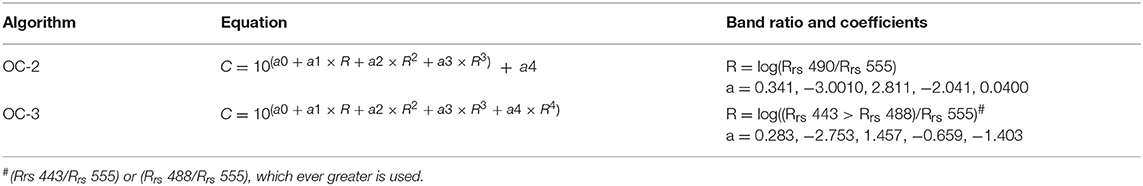
Table 1. Details of the empirical algorithms used for the study (Source: OC-2: O'Reilly et al., 1998; OC-3: Morel and Maritorena, 2001, with OC-3 coefficients for Bay of Bengal from Sarangi, 2016).

Coastal Ocean Monitoring and Prediction System (COMAPS) data used in the present work were available only till the period 2014 for the study area. MSI being a relatively new sensor with data availability only from 2016, the model validation exercise is carried out only for Landsat-8 OLI derived Chl-a. Data used for validation are taken from the samples collected at four stations along Hooghly and Sandheads. The study area map comprising of northern coastal Bay of Bengal is shown in Figure 1. Chl-a averages of the pre-monsoon periods during the years 2014–2017 as retrieved from Landsat-8 OLI using the OC-2 algorithm are overlaid in the background along with the locations of the COMAPS data stations (Figure 1b) The details of the station name, station id, longitude, and latitude are given in Table 2.

FIGURE 1

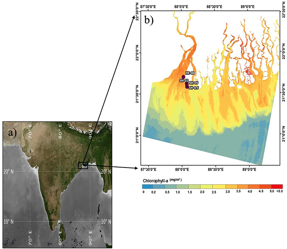
Figure 1. Schematic of the study area: (a) The North Indian Ocean with the domain of interest marked (north coastal Bay of Bengal), (b) Magnified view highlighting the coastal features, locations of the COMAPS data stations, & pre-monsoon averages (2014–2017) of Chl-a retrieved from Landsat-8 OLI using OC-2 algorithm in the background.

TABLE 2

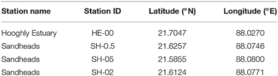
Table 2. Details of the COMAPS station locations used for validation of Chl-a estimated from Landsat-8 OLI.

For the validation exercise, Landsat-8 OLI data geographically collocated with the corresponding in situ observations during the periods December 2013–March 2014 are extracted and converted to R_rs to apply OC-2 and OC-3 algorithms and derive Chl-a. The statistical metrics used for validation were correlation coefficient (r), Root Mean Square Error (RMSE) and bias. The formula for RMSE and bias are given in Equations (4) and (5).

$\begin{array}{ll}RMSE=\sqrt{\frac{{\displaystyle {\sum }_{i=1}^n}{(X_{obs,i}-X_{sensor,i})}^2}{n}}& (4)\end{array}$

$\begin{array}{ll}bias=\frac{1}{n}{\displaystyle \sum _{i=1}^n}(X_{obs,i}-X_{sensor,i})& (5)\end{array}$

where, X_obs,i is the in-situ data obtained and X_sensor,i is the sensor data obtained.

Analysis

Validation of Satellite Derived Chl-a With COMAPS Data

Validation of the OC-2 and OC-3 algorithms in the study region were carried out by comparison with COMAPS in situ data sets. In the study region, COMAPS observations are available only till 2014 which were used in our analysis. For validation of Landsat-8 OLI retrieved Chl-a using the OC-2 and OC-3 algorithms, the OLI observations were geographically collocated with corresponding COMAPS in situ observations during the study period in the study region. The metrics of the statistical analysis performed for retrieving Chl-a using OC-2 and OC-3 algorithms are shown in Table 3. “r,” “bias,” and “RMSE” has been computed for OC-2 and OC-3 algorithms. Chl-a retrieved using OC-2 showed a correlation of 0.795, while Chl-a retrieved using OC-3 had a slightly lower correlation of 0.786. A lower bias and RMSE of 0.350 and 0.737 mg/m³, respectively, were obtained using OC-2. Use of OC-3 algorithm resulted in a higher bias and RMSE of 1.063 and 1.237 mg/m³, respectively. Chl-a estimated using both the algorithms are correlating well with the COMAPS data, however a relatively lower bias and RMSE is observed for OC-2 Chl-a estimations. Further, on considering the entire study region and not just geographically collocated Chl-a, the in situ values (at COMAPS stations) were observed to range between 0.2 and ~8 mg/m³ during post-monsoon to winter periods.

TABLE 3

Table 3. Statistical metrics of validation of Chl-a estimated from Landsat-8 OLI by inter-comparison with in situ (COMAPS) and satellite (MODIS-A) data along with details of in situ Chl-a in the region during this period.

Though our area of interest is the coastal region, a validation exercise was also carried out through inter-comparison of Landsat-8 OLI retrieved Chl-a with MODIS-A derived Chl-a for the region beyond the estuary mouth depending on MODIS data availability. For this, matchups for OLI and MODIS-A during the periods 2013–2014 were obtained for a geographically collocated area chosen within the larger study domain lying between 20°34′38.64″N − 21°30′00″N and 88°24′50.04″E − 91°8′37.68″E. The scatters between the Chl-a retrievals from MODIS-A and OLI sensors are shown in Figure 2. The satellite sensor inter-comparison revealed a better agreement between Chl-a retrieved from MODIS-A and Landsat-8 OLI while using the OC-2 algorithm compared to OC-3 algorithm. The correlation between Chl-a from MODIS-A and OLI is 0.750 for OC-2 retrieval algorithm as against a correlation of 0.713 utilizing the OC-3 algorithm. However, Figure 2 also reveals an overestimation of Chl-a by OLI as compared to MODIS-A and with a larger bias for OC-3 than OC-2. It is pertinent to note this does not mean a better retrieval for any or both of these sensors as compared to in situ measurements, but rather an evaluation of the performance of the OC-2 and OC-3 algorithms for Chl-a retrieval from OLI (30 m spatial resolution) vis-à-vis MODIS-A under similar conditions. The metrics of the statistical intercomparison between MODIS-A and Landsat-8 OLI are also presented in Table 3. Few details of in situ Chl-a in the study region are also presented in the modified Table to provide a limited but realistic overview of Chl-a variability in the region. Validation of Chl-a derived from Landsat-8 using in situ (COMAPS) and satellite (MODIS-A) showed that OC-2 algorithm performs better than OC-3 algorithm. Hence, OC-2 algorithm is used for the estimation of Chl-a and discussed in further sections.

FIGURE 2

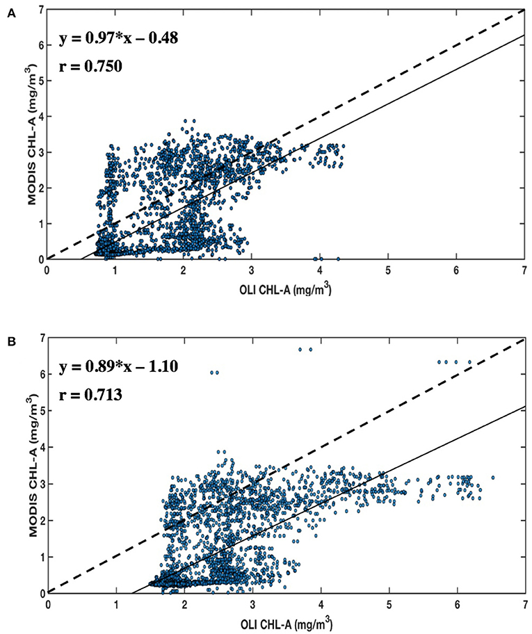
Figure 2. Scatter plots of the Chl-a from MODIS-A vs. Landsat-8 OLI for (A) OC-2 algorithm and (B) OC-3 algorithm, respectively.

Seasonal Variability of Chl-a Estimated Using Landsat-8 OLI

Chlorophyll-a concentration (Chl-a) estimated from Landsat-8 OLI using the OC-2 algorithm for the year 2017 is chosen to study its seasonal variability in the coastal Bay of Bengal (Figure 3). It can be noticed that upstream of Hooghly river and the offshoot of the Ganga-Brahmaputra delta record high Chl-a values throughout the year with winter season recording the highest (>5 mg/m³) followed by the post-monsoon (4–5 mg/m³) and least during the pre-monsoon (3–4 mg/m³). Similar higher concentration of Chl-a can be found near the mouth of the river openings. Irregular patterns of moderate Chl-a distribution varying between 2.5 and 3.5 mg/m³ (during pre-monsoon and post-monsoon) and reaching upto 4 mg/m³ (during winter season) are observed downstream away from the mouth. Chl-a declines in the offshore (0.5–1 mg/m³).

FIGURE 3

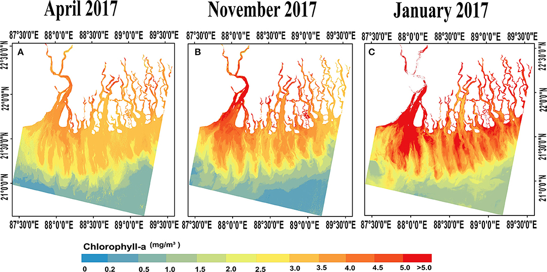
Figure 3. Distribution of Chl-a retrieved from Landsat-8 OLI using the OC-2 algorithm in the northern coastal Bay of Bengal during the year 2017 for (A) pre-monsoon (April), (B) post-monsoon (November), and (C) winter-monsoon (January).

It can be observed that a periodic increase in the Chl-a is observed with the arrival of each season. Variations in Chl-a is in close relation to the river runoff. The maximum runoff observed during the monsoon and post-monsoon period (June–October) deposits the highest concentration of nutrients which favor the phytoplankton growth and hence enhancement of Chl-a. The average values of freshwater discharge for Hooghly are 3,000 m³/s during the southwest monsoon while 1,000 m³/s is discharged during rest of the seasons (Sadhuram et al., 2005). The northern Bay is primarily fed by the Ganga-Brahmaputra-Meghana river system which carries biologically and sediment rich waters during the monsoons. However, winter being a dry season receives very less rainfall over the northern Bay resulting in decreased transport of nutrients by riverine flux for most part near the north of the Bay. However, phytoplankton blooms grow mostly in cooler waters. Despite the presence of nutrients during post-monsoon, enrichment in Chl-a may be found during winter due to the conducive water temperatures along with the presence of pre-deposited nutrients carried by the rivers. The influence of sediments on the optical properties of water is less causing a minimal interference in retrieval of Chl-a during this season. The pre-monsoon season is dry with minimum runoff (both river and agricultural), consequently, a low Chl-a is observed in the region.

Inter-comparison of Chl-a From Sentinel-2 MSI and Landsat-8 OLI

In this section, Chl-a estimated from the two sensors, Sentinel-2 MSI and Landsat-8 OLI are intercompared during their overlapping year 2017. Inter-comparison of the sensors is done on a sub-section of the study area lying in between 20°47′44.062″N-21°40′59.754″N and 87°28′36.323″E-89°1′13.385″E as shown in the Figure 1b which also accommodates the COMAPS in situ observation stations. Chl-a during the three seasons, pre-monsoon, post-monsoon, and winter season is shown in Figure 4. It can be observed that Chl-a values from Sentinel-2 MSI are overestimated compared to those from Landsat-8 OLI during April and November. However, during the winter season (January), Chl-a retrieved from Sentinel-2 MSI are underestimated when compared to Chl-a retrieved from Landsat-8 OLI over the same region. This difference in retrieved Chl-a values from the two different sensors even though using the same retrieval algorithms could be attributed to the use of same retrieval coefficients for rather two functionally different sensors (MSI vs. OLI).

FIGURE 4

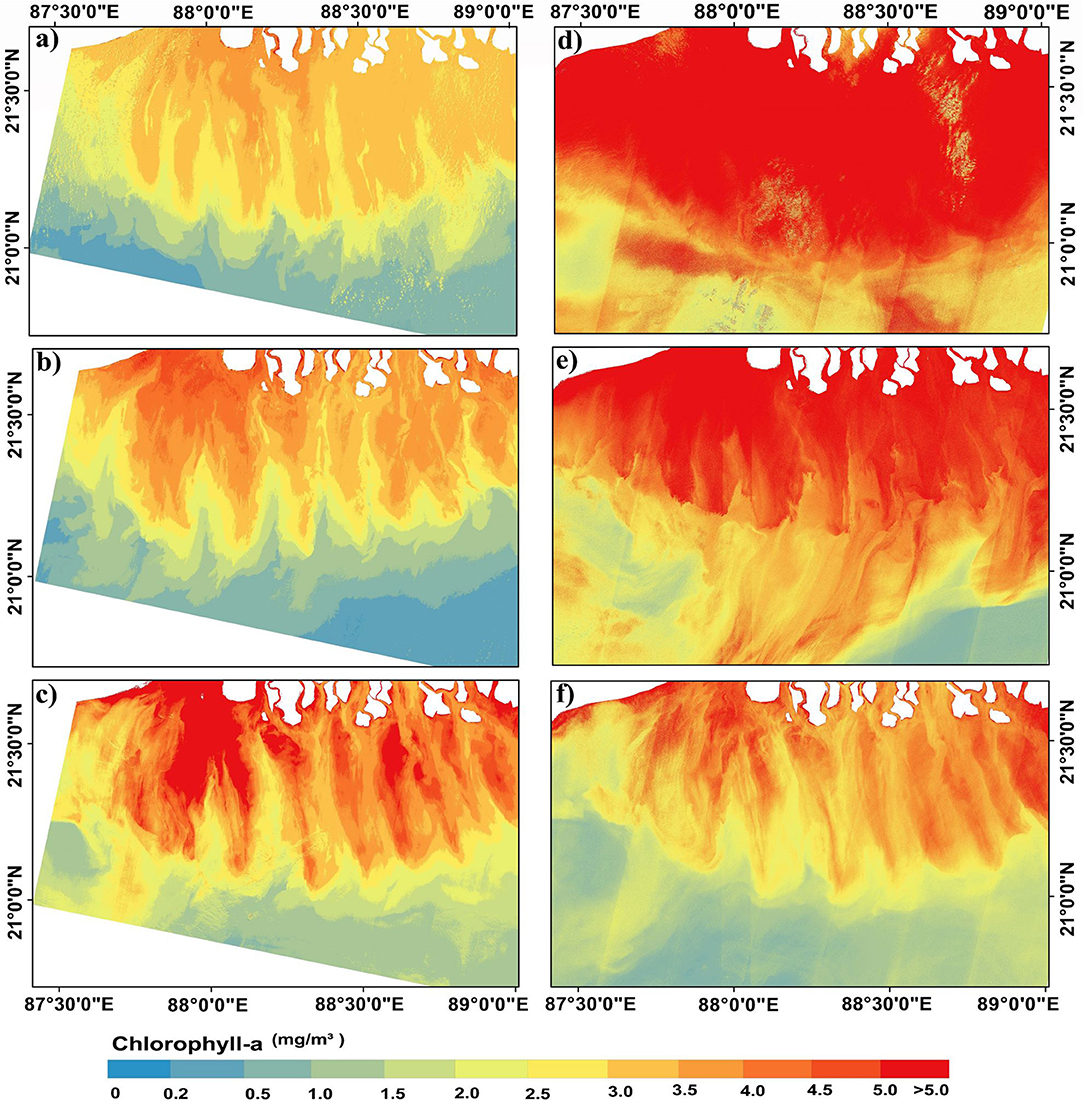
Figure 4. Seasonal distribution of Chl-a during 2017 estimated from (a–c) Landsat-8 OLI, and (d–f) Sentinel-2 MSI.

During the pre-monsoon season the Chl-a traced by OLI exhibits a distinct pattern that is not traced by MSI sensor. The distribution clearly indicates a possible saturation in case of MSI sensor with Chl-a values far >5 mg/m³ almost in the entire study region. Very close to the Hooghly river mouth, the Chl-a values for OLI sensor lies in the range 3–4 mg/m³ while for MSI sensor Chl-a values >5 mg/m³ is found covering most of the study area. Irregular patterns of low and high Chl-a are seen upto 21°N for both the sensors beyond which values decrease upto 0.5 and 2–3 mg/ m³ for OLI and MSI, respectively. Unlike the pre-monsoon season, the patterns traced by both the sensors is similar. Near the mouth of the estuary the value traced by the OLI sensor lies from 3.5 to 4.5 mg/m³ while extremely high values of Chl-a ranging >5 mg/m³ is traced by MSI upto 21° 30′ N. Beyond this, it was observed that Chl-a traced by MSI varies from 2.5 to 3.5 mg/m³ while OLI sensor could record values from 1.0 to 2.5 mg/m³. During the winter season there is a noticeable shift in the Chl-a traced by both the sensors than the previous months. Very high values of Chl-a >4 mg/m³ could be traced near the Hooghly estuarine mouth for both the sensors. The values change evolving into distinct patterns near the coast. Chl-a values range from 2.5–4.5 to 1.5–2.5 mg/m³ near 21° N, and going to <1.5 mg/m³ beyond it. Similarity in pattern as well as values for Chl-a traced by OLI sensor could be identified for the MSI sensor. It could be stated that beyond 21°N latitude the Chl-a value decreases for both the sensors.

Figure 5 shows the scatters between OLI and MSI for the three different seasons analyzed. Statistical parameters viz. correlation coefficients (r), RMSE and bias were calculated using the formula stated in Equations (4) and (5), respectively, and are given in Table 4. It can be noted that the highest correlation between Chl-a from MSI and OLI is observed for the month of January (winter-monsoon) at 0.874 and the lowest correlation is observed for the month of April (pre-monsoon; 0.438). A strong bias between the Chl-a estimated from the two sensors was observed with the highest being in April (3.095 mg/m³) and lowest (−0.455 mg/m³) during the month of January. The highest error (3.368 mg/m³) generated using OC-2 was observed for the April month corresponding to the pre-monsoon season showing appreciable mismatch among the sensors. Post-monsoon season represented by the month of November has a good correlation of 0.833 with a moderate bias and RMSE of 1.601 and 1.738 mg/m³.

FIGURE 5

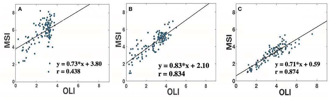
Figure 5. Scatter plots of the Chl-a estimated from Landsat-8 OLI and Sentinel-2 MSI for (A) pre-monsoon (April), (B) post-monsoon (November), and (C) winter-monsoon (January), respectively, during the year 2017.

TABLE 4

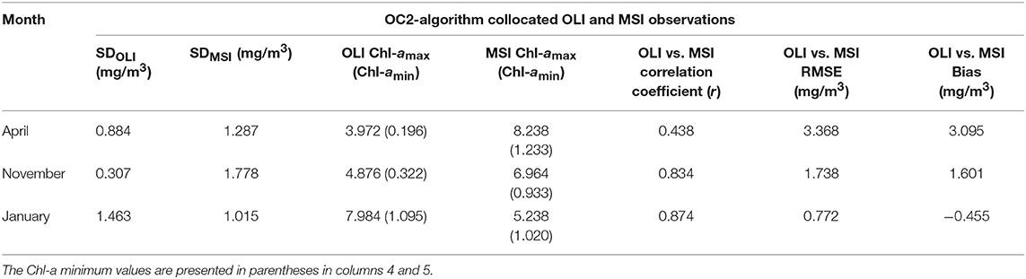
Table 4. Descriptive statistics of the scatters between Chl-a retrieved from OLI (Landsat-8) and MSI (Sentinel-2) using OC2 algorithm.

Conclusions

Northern coastal region is one of the highly productive regions in the Bay of Bengal. Agricultural and river runoff deposit nutrients favorable for phytoplankton growth in this region. Two bio-optical algorithms, OC-2 and OC-3 were used to assess the performance of Chl-a estimation from fairly good-spatial resolution sensors Landsat-8 OLI and Sentinel-2 MSI. Results showed that the OC-2 algorithm was able to estimate Chl-a in the northern coastal region reasonably well and was performing better than OC-3 algorithm for OLI. Seasonal variability of Landsat-8 OLI derived Chl-a was analyzed and it was observed that Chl-a increased with the arrival of monsoon season. It was further observed that Chl-a was lowest for the month of April and highest in the month of January (winter season). Seasonality of Chl-a could be closely related to the riverine flux of the Ganga-Brahmaputra-Meghana river systems. Inter-comparison of Chl-a retrieved from the two sensors (Landsat-8 OLI and Sentinel-2 MSI) was then carried out during their overlapping year 2017. From the analysis, substantial difference was observed in Chl-a estimated by both the sensors. Sentinel-2 MSI was found to overestimate Chl-a compared to Landsat-8 OLI, most of the time. The present analysis clearly indicated the need for continuous time series in situ observations for Case-2 waters at several stations. Additionally, sensor inter-comparison and validation exercises for improving the accuracy of Chl-a estimations from satellite based sensors of varying spatial resolutions as well as the need for improved bio-optical algorithms could be well-recognized for the study region.

Data Availability Statement

The datasets analyzed for this study can be found in the [USGS (https://earthexplorer.usgs.gov/), scihub (https://scihub.copernicus.eu), Ladsweb (https://ladsweb.modaps.eosdis.nasa.gov/search/), and in-situ COMAPS data is available on request from ICMAM Project Directorate NCCR, MoES, Govt. of India].

Author Contributions

SP was responsible for carrying out the work presented in the manuscript. NC conceived the idea of the work in consultation with DS. DS was responsible for providing useful insights during various stages of the work. All the authors contributed in the discussions of the results and drafting the manuscript.

Funding

No specific funding support has been received for carrying out this work. However, one of the authors, SP was supported by MHRD through a GATE fellowship as part of her academic degree programme.

Conflict of Interest

The authors declare that the research was conducted in the absence of any commercial or financial relationships that could be construed as a potential conflict of interest.

Acknowledgments

The authors of this paper would like to thank Indian National Centre for Ocean Information Services (INCOIS) and Integrated Coastal and Marine Area Management (ICMAM) Project Directorate/MoES for providing the data under Coastal Ocean Monitoring and Prediction System (COMAPS) programme for validation purposes. Dr. Ch, Jayaram (RRSC-E, NRSC) is gratefully acknowledged for valuable technical inputs.

Supplementary Material

The Supplementary Material for this article can be found online at: https://www.frontiersin.org/articles/10.3389/fmars.2019.00598/full#supplementary-material

References

Antoine, D., Morel, A., Gordon, H. R., Banzon, V. F., and Evans, R. H. (2005). Bridging ocean colour observations of the 1980s and 2000s in search of long-term trends. J. Geophys. Res. 110, 1–22. doi: 10.1029/2004JC002620

CrossRef Full Text | Google Scholar

Blondeau-Patissier, D., Gower, J. F. R., Dekker, A. G., Phinn, S. R., and Brando, V. E. (2014). A review of ocean color remote sensing methods and statistical techniques for the detection, mapping and analysis of phytoplankton blooms in coastal and open oceans. Progr. Oceanogr. 123, 123–144. doi: 10.1016/j.pocean.2013.12.008

CrossRef Full Text | Google Scholar

Boucher, J., Weathers, K. C., Norouzi, H., and Steele, B. (2018). Assessing the effectiveness of Landsat 8 chlorophyll: a retrieval algorithms for regional freshwater monitoring. Ecol. Appl. 28, 1044–1054. doi: 10.1002/eap.1708

PubMed Abstract | CrossRef Full Text | Google Scholar

Chauhan, P., Mohan, M., Nayak, S. R., and Navalgund, R. R. (2002). Comparison of ocean color chlorophyll algorithms for IRS-P4 OCM sensor using in-situ data. J. Indian Soc. Remote Sens. 30, 87–94. doi: 10.1007/BF02989980

CrossRef Full Text | Google Scholar

Concha, J. A., and Schott, J. R. (2014). “In-water component retrieval over Case 2 water using Landsat 8: initial results,” in 2014 IEEE Geoscience and Remote Sensing Symposium (Québec City, QC).

Google Scholar

Concha, J. A., and Schott, J. R. (2016). Retrieval of color producing agents in Case 2 waters using Landsat 8. Remote Sens. Environ. 185, 95–107. doi: 10.1016/j.rse.2016.03.018

CrossRef Full Text | Google Scholar

Dwivedi, S. N. (1993). “Long-term variability in the food chains, biomass yield, and ocenaography of the Bay of Bengal eco-system,” in Large Marine Ecosystems: Stress, Mitigation, and Sustainability, eds K. Sherman, L. M. Alexander, and B. D. Gold (Washington, DC: American Association for the Advancement of Science, 43–52.

Google Scholar

ESA-European Space Agency (2015). Sentinel-2A spectral response functions (S2A-SRF): COPE-GSEG-EOPG-TN-15–0007.

Google Scholar

Hooker, S. B., McClain, C. R., and Holmes, A. (1993). Ocean colour imaging–CZCS to SeaWiFS. Mar. Technol. Soc. J. 27, 3–15.

Google Scholar

IOCCG (2000). “Remote sensing of ocean colour in coastal, and other optically-complex, waters,” in Reports of the International Ocean-Colour Coordinating Group, No. 3, ed S. Sathyendranath (Dartmouth, NS: IOCCG).

Google Scholar

Kaisary, S., Babu, K. N., Balasubramanian, T., Dileep Kumar, M., Patra, S., Sundaramoorthy, S., et al. (2012). Coastal Water Quality Measurements Protocol for COMAPS Programme. ICMAM Technical report, National Centre For Coastal Research (NCCR), Ministry of Earth Sciences, Govt. of India. 110.

Google Scholar

Lee, Z., Carder, K., Arnone, R., and He, M.-X. (2007). Determination of primary spectral bands for remote sensing of aquatic environments. Sensors 7, 3428–3441. doi: 10.3390/s7123428

PubMed Abstract | CrossRef Full Text | Google Scholar

Madeswaran, P., Ramana Murthy, M. V., Rajeevan, M., Ramanathan, V., Patra, S., Sivasdas, S. K., et al. (2018). Status Report: Seawater Quality at Selected Locations Along Indian Coast. NCCR Publication. 177.

Google Scholar

Mobley, C. D., Stramski, D., Bissett, W. P., and Boss, E. (2004). Optical modeling of ocean waters: is the case 1–case 2 classification still useful? Oceanography 17, 60–67. doi: 10.5670/oceanog.2004.48

CrossRef Full Text | Google Scholar

Moran, M. S., Jackson, R. D., Slater, P. N., and Teillet, P. M. (1992). Evaluation of simplified procedures for retrieval of land surface reflectance factors from satellite sensor output. Remote Sens. Environ. 41, 169–184. doi: 10.1016/0034-4257(92)90076-V

CrossRef Full Text | Google Scholar

Morel, A., and Maritorena, S. (2001). Bio-optical properties of oceanic waters: a reappraisal. J. Geophys. Res. 106, 7163–7180. doi: 10.1029/2000JC000319

CrossRef Full Text | Google Scholar

Moses, W. J., Bowles, J. H., and Corson, M. R. (2015). Expected improvements in the quantitative remote sensing of optically complex waters with the use of an optically fast hyperspectral spectrometer-a modeling study. Sensors 15, 6152–6173. doi: 10.3390/s150306152

PubMed Abstract | CrossRef Full Text | Google Scholar

Mukhopadhyay, S. K., Biswas, H., De, T. K., and Jana, T. K. (2006). Fluxes of nutrients from the tropical River Hooghly at the land–ocean boundary of Sundarbans, NE Coast of Bay of Bengal, India. J. Marine Syst. 62, 9–21. doi: 10.1016/j.jmarsys.2006.03.004

CrossRef Full Text | Google Scholar

NASA (2011). Landsat 7 Science Data Users Handbook Landsat Project Science Office at NASA's Goddard Space Flight Center in Greenbelt. 186. Available online at: http://landsat.gsfc.nasa.gov/wp-content/uploads/2016/08/Landsat7_Handbook.pdf (accessed May 5, 2019).

Google Scholar

Nechad, B., Ruddick, K., Schroeder, T., Oubelkheir, K., Blondeau-Patissier, D., Cherukuru, N., et al. (2015). CoastColour Round Robin data sets: a database to evaluate the performance of algorithms for the retrieval of water quality parameters in coastal waters. Earth Syst. Sci. Data 7, 319–348. doi: 10.5194/essd-7-319-2015

CrossRef Full Text | Google Scholar

Ngoc, D. D., Loisel, H. L., Jamet, C., Vantrepotte, V., Duforêt-Gaurier, L., Minh, C. D., et al. (2019). Coastal and inland water pixels extraction algorithm (WiPE) from spectral shape analysis and HSV transformation applied to Landsat 8 OLI and Sentinel-2 MSI. Remote Sens. Environ. 223, 208–228. doi: 10.1016/j.rse.2019.01.024

CrossRef Full Text | Google Scholar

O'Reilly, J. E., Maritorena, S., Mitchell, B. G., Siegal, D. A., Carder, K. L., Graver, S. A., et al. (1998). Ocean color chlorophyll algorithms for SeaWiFS. J. Geophys. Res. 103, 24937–24953. doi: 10.1029/98JC02160

CrossRef Full Text | Google Scholar

O'Reilly, J. E., Maritorena, S., O'Brien, M. C., Siegel, D. A., Toole, D., Menzies, D., et al. (2000). “SeaWiFS post-launch calibration and validation analysis, part 3,” in NASA Technical Memorandum−2000–206892, Vol. 11, eds S. B. Hooker and E. R. Firestone (Maryland: NASA Goddard Space Flight Center), 49.

Google Scholar

Rakshit, D., Biswas, S. N., Sarkar, S. K., Bhattacharya, B. D., Godhantaraman, N., and Satpathy, K. K. (2014). Seasonal variations in species composition, abundance, biomass and production rate of tintinnids (Ciliata: Protozoa) along the Hooghly (Ganges) River Estuary, India: a multivariate approach. Environ. Monit. Assess. 186, 3063–3078. doi: 10.1007/s10661-013-3601-9

PubMed Abstract | CrossRef Full Text | Google Scholar

Sadhuram, Y., Sarma, V. V., Ramana Murthy, T. V., and Prabhakara Rao, P. B. (2005). Seasonal variability of physico-chemical characteristics of the Haldia channel of Hooghly Estuary, India. J. Earth Syst. Sci. 114, 37–49. doi: 10.1007/BF02702007

CrossRef Full Text | Google Scholar

Sarangi, R. K. (2016). Remote sensing observations of ocean surface chlorophyll and temperature with the impact of cyclones and depressions over the Bay of Bengal water. Mar. Geodesy. 39, 53–76. doi: 10.1080/01490419.2015.1121172

CrossRef Full Text | Google Scholar

Sarangi, R. K., Chauhan, P., Mohan, M., Nayak, S. R., and Navalgund, R. R. (2001). Phytoplankton distribution in the Arabian Sea using IRS-P4 OCM satellite data. Int. J. Remote Sens. 22, 2863–2866. doi: 10.1080/01431160119527

CrossRef Full Text | Google Scholar

Subramanian, V. (1993). Sediment load of Indian Rivers. Curr. Sci. 64, 928–930.

Google Scholar

Vuolo, F., Zółtak, M., Pipitone, C., Zappa, L., Wenng, H., Immitzer, M., et al. (2016). Data service platform for sentinel-2 surface reflectance and value-added products: system use and examples. Remote Sens. 8, 1–16. doi: 10.3390/rs8110938

CrossRef Full Text | Google Scholar

Watanabe, F., Alcantara, E., Rodrigues, T., Rotta, L., Bernardo, N., and Imai, N. (2017). Remote sensing of the chlorophyll-a based on OLI/Landsat-8 and MSI/Sentinel-2A (Barra Bonita reservoir, Brazil). An. Acad. Bras. Ciênc. 90, 1987–2000. doi: 10.1590/0001-3765201720170125

PubMed Abstract | CrossRef Full Text | Google Scholar