Estimating Carbon Flux From Optically Recording Total Particle Volume at Depths Below the Primary Pycnocline

Introduction

Imaging systems have been used to characterize plankton and particles in the sea for many decades. Examples are the original film-based systems by Asper (1987), Walsh and Gardner (1992), MacIntyre et al. (1995), and Jackson et al. (1997). More recently, recordings have been made digitally, and some systems are available commercially (Stemmann et al., 2004 and references listed in their Table 1; Cowen and Guigand, 2008; Ohman et al., 2019). Other imaging systems rely on holography in various configurations (inline and off-axis), with their own advantages (e.g., large depth of field and survey volumes) and disadvantages (e.g., additional processing for image reconstruction) (Malkiel et al., 1999; Watson et al., 2001; Xu et al., 2001; Bochdansky et al., 2013; Lindensmith et al., 2016).

In contrast to other optical systems such as transmissometry, optical backscattering, forward scattering laser diffraction, and fluorometry, particle imaging systems allow a much more detailed analysis of particle morphology such as size, aspect ratio, roughness, and porosity using relatively simple image-analytical procedures. Image surveys can further be expanded to the classification of particles. For instance, zooplankton can be distinguished from marine snow and fecal pellets, all of which have different settling or migration rates through the water column. We are now at a threshold where machine learning will greatly improve throughput in the classification of particles once trained on specific targets by expert human operators (e.g., Zheng et al., 2017; Luo et al., 2018). Therefore, imaging systems can accurately survey relatively rare macroscopic particles in areas such as the deep sea where other optical systems such as optical backscatter or transmissometry reach their lower detection thresholds (Bochdansky et al., 2016).

Imaging systems were also developed that use fluorometers on moored arrays (McGill et al., 2016) or transmissometers on free-floating sediment traps (Estapa et al., 2017) as “optical sediment traps” which are a suitable match to the neutrally buoyant sediment traps that collect particulate organic carbon (Valdes and Price, 2000). While these latter systems represent direct flux measurements, the question remains how much can be learned from the standing stock of particles as detected by water column imaging systems alone. These comparisons go back at least to Walsh and Gardner (1992) when sediment trap fluxes were compared to aggregate abundance at various depths. More recently, studies concluded that carbon flux compared well with standing stocks of particles in the water column by either applying models based on particle-size spectra (Guidi et al., 2008), or even more favorably by using locally calibrated sinking fluxes for specific particle size ranges in combination with gel traps (McDonnell and Buesseler, 2012).

To understand what data from imaging systems tell us about the biological pump, we need to compare them with POC estimates derived from other methods, and explore how a snapshot of the standing stock of particles in the water column correlates with export flux. Exploring the connection between particle abundance at the surface and at mesopelagic depths, we use data from two research expeditions; one to the North Atlantic in the summer of 2012 and one to the Ross Sea from February to March of 2013. Both regions are characterized by seasonally high export production of global significance (Arrigo et al., 1999; Sanders et al., 2014). In addition, the Ross Sea data allowed us to compare seasonally integrated export fluxes based on seasonal net community production (sNCP) and upper water column carbon mass balance to particle inventories and water column characteristics in four distinct regions on the Ross Sea shelf.

Materials and Methods

Research Expedition Details

Subarctic North Atlantic and Arctic Ocean

Data were collected on the RV Pelagia (Royal Netherlands Institute for Sea Research) during the MEDEA expedition between June 22 and July 22, 2012. Most stations were within the subarctic North Atlantic while three stations were located in the Norwegian Sea, Arctic Ocean (Figure 1A). Physical characteristics (conductivity, temperature, and pressure) of the water column was measured with a Seabird SBE9/11+ conductivity, temperature, and depth (CTD) probe. Factory calibrations of the conductivity and oxygen sensors were checked for stability with appropriate reference samples measured on board. Salinity standards and samples were measured with a Guildline 8400B salinometer. The CTD was lowered at ∼1 m s^–1.

FIGURE 1

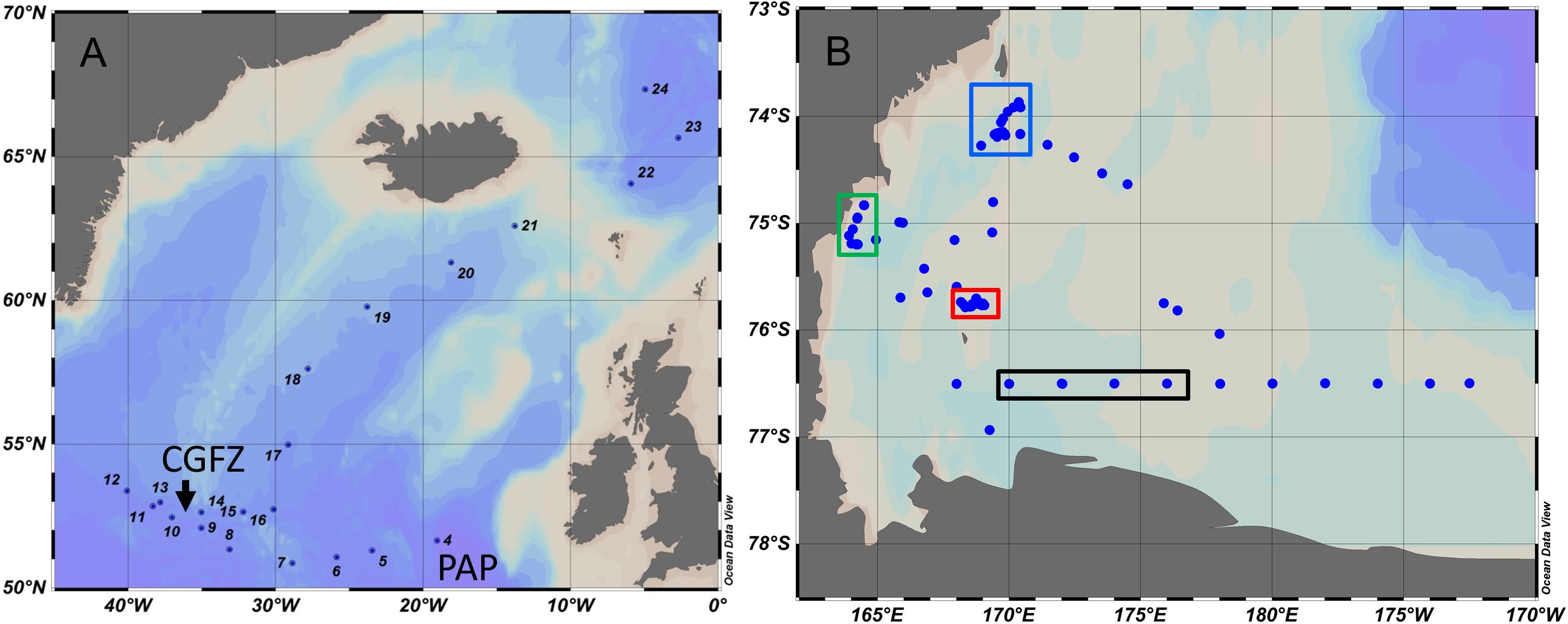
Figure 1. Stations occupied in the North Atlantic (June–July 2012) (A) and the Ross Sea (February–March 2013) (B). CGFZ, Charlie Gibbs Fracture Zone is a pair of deep-sea trenches characterized by a thriving benthic community due to high primary productivity and export of organic carbon to deeper layers. PAP, Porcupine Abyssal Plain. During the Ross Sea expedition NBP1302, we revisited three areas indicated by red, green, and blue rectangles. The black rectangle shows the four 76° 30′ transect stations used in this analysis.

Ross Sea

For the Ross Sea, we focused our analysis on three sites that were reoccupied multiple times during the cruise, and a zonal transect. Data were collected on the RVIB Nathaniel B Palmer from February 12 to March 18, 2013 (cruise designation NBP-1302). The main focus was on the western Ross Sea (Figure 1B) as it represents a significant site for Antarctic Bottom Water formation (Orsi et al., 2002) and also hosts significant phytoplankton blooms between late spring and early autumn. We focused on three areas in the western Ross Sea: north of Franklin Island (“south site”), south of Coulman Island (“north site”), and Terra Nova Bay (TNB), each revisited several times during the expedition to record temporal changes (DeJong et al., 2017). TNB was the site of highest drawdown of inorganic carbon of all sites visited during this expedition (DeJong et al., 2017). The zonal transect was along the 76° 30′ S line (Figure 1B), a section visited during many previous research cruises (e.g., Carlson et al., 2000; Smith et al., 2013). The CTD with instruments was lowered at 0.5 m s^–1 for the first 100 m, and then accelerated to 1 m s^–1 for the remainder of each cast. Salinity, temperature, and oxygen measurements were obtained using SeaBird 911+ CTD probes. Salinity was calibrated on discrete samples at 24°C using a Guildline 8400 Autosal four-electrode salinometer. The station maps were created using Ocean Data View (Schlitzer, 2018).

Video Particle Profiler

The Video Particle Profiler (VPP) was previously described in Bochdansky et al. (2017). Side lighting with two white high-intensity LED lights [Fenix L2P, powered by a 2.4 V, 35 Ah NiMH battery pack (custom built by Batterspace/AA Portable Power Corp.)] was used ∼7 cm in front of the sapphire window of a pressure case rated to 6000 m (Supplementary Figure 1), containing a Sentec monochrome video camera (Model STC-160BT2, VGA resolution, 640 × 480 pixels). At the focal plane, the field of view was 3.5 and 4.7 cm. The light beams were spatially filtered using 1 cm slits, however, only the brightest lit image plane was used for analysis in the exponentially decaying light field. Identical hardware and software configurations were used for all stations during both cruises. As the gray-level threshold was subjective, no precise image volume can be determined, and thus particle abundances are reported as particles per image frame, or cubic pixels per image frame (see Supplementary Figure 2 for examples). This selectivity during image analysis reduced bias caused by overlapping particles while providing more precise particle-size measurements. Each image pixel spans 0.034 mm in length with an area of 0.00116 mm². To avoid noise caused by random single-pixel electronic “snow,” the threshold for being considered a true particle was set at a 6-pixel minimum using eight-connectivity. It follows that the minimum size of a particle considered in this analysis translated to particles of a size of 2 × 3 or 1 × 6 pixels, equal to 68 × 102 or 34 × 204 μm, respectively. The VPP records 30 images per second that were analyzed with a custom Linux-based program (an adapted Avidemux video editing software in Ubuntu) after retrieval (see Supplementary Material for links to the open-source program and image analysis code used in this analysis). Image data were aligned in Matlab with depth from the CTD using a common time stamp at 1 s (∼1 m) resolution. The projected area of the particle (sum of white and black pixels within the perimeter of the particle determined by eight-connectivity) was converted to a circle that was then converted to the volume of a sphere (Iversen et al., 2010; Bochdansky et al., 2017). To obtain total volumes (pixel³ frame^–1), volumes of particles were summed for each frame and the average total volume was calculated for each meter, and then again averaged over the depth ranges (50–60 or 200–300 m).

Chlorophyll Fluorescence

In situ chlorophyll fluorescence during the MEDEA and Ross Sea expeditions was determined using Wetlabs ECO fluorometers.

Particulate Organic Carbon, Total Dissolved Inorganic Carbon, and Dissolved Organic Carbon (Ross Sea Only)

Details of POC and ΣCO₂ collection and analysis were previously published in DeJong et al. (2017). Between 0.5 and 4 L of seawater were filtered through combusted Whatman GF/C filters for POC analysis. Filters were rinsed with 0.1 N HCl, air dried, and analyzed using a Carlo Erba NA1500 Series elemental analyzer coupled with a Finnigan Delta + mass spectrometer with a ConFlo ll open split interface (DeJong et al., 2017). ΣCO₂ samples were collected in glass BOD bottles and analyzed shipboard within 6–12 h. From each sample, 1.5 ml was analyzed in triplicates after acidification with phosphoric acid, bubble stripping, mass flow control, and using a LICOR-based detection system for CO₂ mass integration (DeJong et al., 2017). DOC was determined using high temperature oxidation (Dickson et al., 2007).

Coulter Counter

Approximately 20 ml water samples were directly taken from the Niskin bottles in 25 ml polystyrene blood cell counting vials with lids. Particles were counted in 0.5 ml increments using a model Z2 Coulter counter. Seven counts were performed on each sample, the first discarded, and then the remaining six counts averaged. The method is based on electrical impedance when a particle passes a pore between two electrodes. For each station, deep-sea samples were counted first and surface samples last to avoid cross-contamination. Before and after each cast the glass aperture was cleaned with 0.2 μm filtered deep-sea water until blank values were at zero. The Coulter counter was calibrated using 5 μm diameter Coulter counter calibration size standard L5 beads (Beckman Coulter). The number of pulses represent the number of particles, and the size of the spike is proportional to particle size. The entire counter was wrapped in a brass grid (~0.5 cm open squares) that was additionally covered with aluminum foil to function as a Faraday cage, preventing noise from electric systems on board. In addition, the door of the counter was bonded to the ship’s ground. During the North Atlantic expedition, we analyzed a size range from 2 to 6 μm. This size range, however, was associated with excessive electronic noise in the lowest size channels despite taking the precautions mentioned above. We therefore abandoned the channels between 2 and 3 μm during the Ross Sea expedition, and used a size range between 3 and 10 μm instead, reducing blank values (deep-sea water filtered through a 0.2-μm syringe filter) to zero or to the lower single digits so that no blank correction was needed.

Estimates of Seasonal Carbon Export Using Upper Water-Column Mass Balance (Ross Sea Only)

Data on seasonal export were taken directly from the Supplementary Materials of DeJong et al. (2017). Briefly, seasonal export was calculated by carbon mass balance: subtracting surplus water-column standing stocks of total particulate organic carbon from the estimated sNCP:

$$\text{sExport}=\text{sNCP}-\mathrm{Surp}(\mathrm{TOC})(1)$$

sNCP was estimated by adding the deficit in dissolved inorganic carbon [Def(nDIC)] to the integrated CO₂-flux from the beginning of the season (November 1) to the arrival time at the cast:

$$\text{sNCP}=\text{Def}(n\mathrm{DIC})+\underset{\text{Nov}1}{\overset{\text{arrival}}{\int }}({\text{CO}}_2\text{flux})\text{d}t(2)$$

CO₂-flux was determined by

$${\text{CO}}_2\text{flux}=(1-A)ks(\mathrm{\Delta }{\text{pCO}}_2),(3)$$

where A is the proportion of sea ice cover, k the CO₂ gas transfer velocity calculated by using squared wind velocity and the temperature-dependent Schmidt number according to Wanninkhof (1992), and s is the solubility term as a function of temperature and salinity (Weiss, 1974).

Surplus DOC and POC from pre-bloom conditions [Surp(TOC) = Surp(DOC) + Surp(POC)] in Eq. 1 were calculated by adding POC and DOC integrated over the top 200 m consistent with Sweeney et al. (2000)

$$\text{Surp}(X)=\underset{0\text{m}}{\overset{200\text{m}}{\int }}(X(\mathrm{late}\mathrm{summer}))\text{d}z-\underset{0\text{m}}{\overset{200\text{m}}{\int }}(X(winter))\text{d}z,(4)$$

where X is either DOC or POC. More detail can be found in DeJong et al. (2017).

Choice of Depth Intervals for Estimating Export

Depth intervals of 50–60 and 200–300 m were used previously in a comparison between upper and deeper water particle abundance across 77 stations visited during the Ross Sea cruise (Bochdansky et al., 2017). In our optical configuration the camera was exposed to ambient light that resulted in light contamination at the surface. Below 50 m, however, casts at all stations could be used. The 50–60 m interval was therefore used as a reliable shallow depth interval. The 200–300 m depth layer was well below the main pycnocline in all casts in both regions and particles arriving at this depth can safely be considered exported as this depth is well below euphotic zone and mixed layer depths (Giering et al., 2017). The 200–300 m depth interval was also below the depth range used in the calculations of export in Sweeney et al. (2000) and Long et al. (2011), and well below export depths typically defined for the ²³⁴Th method, either as the bottom of the euphotic zone (Buesseler and Boyd, 2009), equilibrium depth (Lemaitre et al., 2018), or as 100 m (Maiti et al., 2013; Le Moigne et al., 2016). Importantly, and to allow for direct comparison, particle flux beyond 200 m was also used by DeJong et al. (2017) to define export (see above).

Results

Particle abundance changed greatly across the subarctic North Atlantic and the Ross Sea during both expeditions (Figure 2), providing a wide dynamic range in interpreting particle abundances with depth, and as dependent on water column characteristics. For the North Atlantic expedition, we divided the stations (Figure 1) into seven sets. One set was located east of the Charlie Gibbs Fracture Zone (CGFZ, Figure 1), two sets delineated the southern and northern branch of the CGFZ; one station was located west of the CGFZ (station #12). Station 17, with its extreme density stratification, was kept separate for this analysis. A set of four stations (#18–21) were positioned on a trajectory north toward the Iceland-Faroe Ridge before entering the Arctic Ocean. Three CTD casts and one VPP cast were taken in the Norwegian Sea (Arctic Ocean) (Figure 1). The density structure was very different in the Arctic basin with considerably higher sigma-t values overall than those observed in the subarctic North Atlantic (Figure 2). Nepheloid layers close to the bottom were prominent in almost all casts in both cruises (Figure 2). Note that the scales for particle abundance in Figure 2 are different for the North Atlantic and the Ross Sea so that by comparison the Ross Sea nepheloid layers appear less pronounced than in the North Atlantic but in fact are equivalent in magnitude. In the North Atlantic at Station 16, the nepheloid layer reached 300 m in depth from the ocean bottom. In the Ross Sea, there was a gradient in surface particle abundance from high numbers at TNB (green) to the north site (blue), to the transect stations (black), to low particle abundances at the south site (red) (Figure 2D). In terms of total particle volumes, the difference between the north site and TNB was greatly reduced with approximately the same total particle volumes in the surface at both stations (insert in Figure 2D). At 100–300 m water depths, however, total particle volumes were much higher in TNB than at the north site.

FIGURE 2

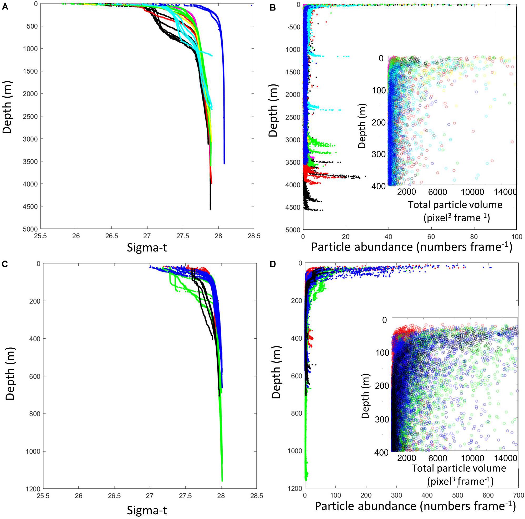
Figure 2. Density (Sigma-t) and particle abundance (numbers per video frame), respectively, during the North Atlantic (A,B) and the Ross Sea (C,D) expeditions. The insets show a close-up of total particle volume (pixel³ frame^{– 1}). Total particle volume is a better predictor of particle carbon than is particle abundance because average particle volume changed with depth. Note that particle abundances are plotted at different scales for the two regions, with the open North Atlantic having lower abundance than the Ross Sea. Pronounced benthic nepheloid layers were present in most casts in both regions. Color codes of data points in the North Atlantic (A): black, stations east of the Charlie Gibbs Fracture Zone (CGFZ); red, southern trench of the CGFZ; magenta, station 12 west of the CGFZ; green, northern trench of the CGFZ; yellow, station 17; cyan, stations 18–21; blue, Norwegian Sea, Arctic. Color codes of data points in the Ross Sea (B): red, south site; green, Terra Nova Bay; blue, north site; black, transect stations.

There is a significant relationship between total particle volume at 50–60 and at 200–300 m in both expeditions (Figure 3). Where residuals were not normally distributed, p-values were based on custom F-distributions obtained by data randomization (10,000×) (Manly, 2007). A custom F-distribution based on randomization of the actual data produces an accurate p-value independent of the normality assumption employed by standard statistical tables. The linear regression between total volume at 50–60 m and at greater depth for the North Atlantic is y = 302 + 0.153x, n = 18, r² = 0.375, p = 0.022 (Figure 3A). For the Ross Sea, the regression equation for total volumes between the same depth ranges is: 667 + 0.0856x, r² = 0.197, p = 0.0074 (Figure 3C). The south site had low total particle volumes at 200–300 m, consistent with low total volumes at the surface. At the north site, mesopelagic total particle volumes were much lower compared to upper layers (Figure 3C). At TNB, total particle volumes were both high at the surface and at depth (Figure 3C). The total volumes during the transect stations were relatively low at the surface, but not as low as the values at the south site (Figure 3C). Deep-water total particle volumes at the transect stations fell consistently below the regression line, indicating a lack of export at these sites (Figure 3C).

FIGURE 3

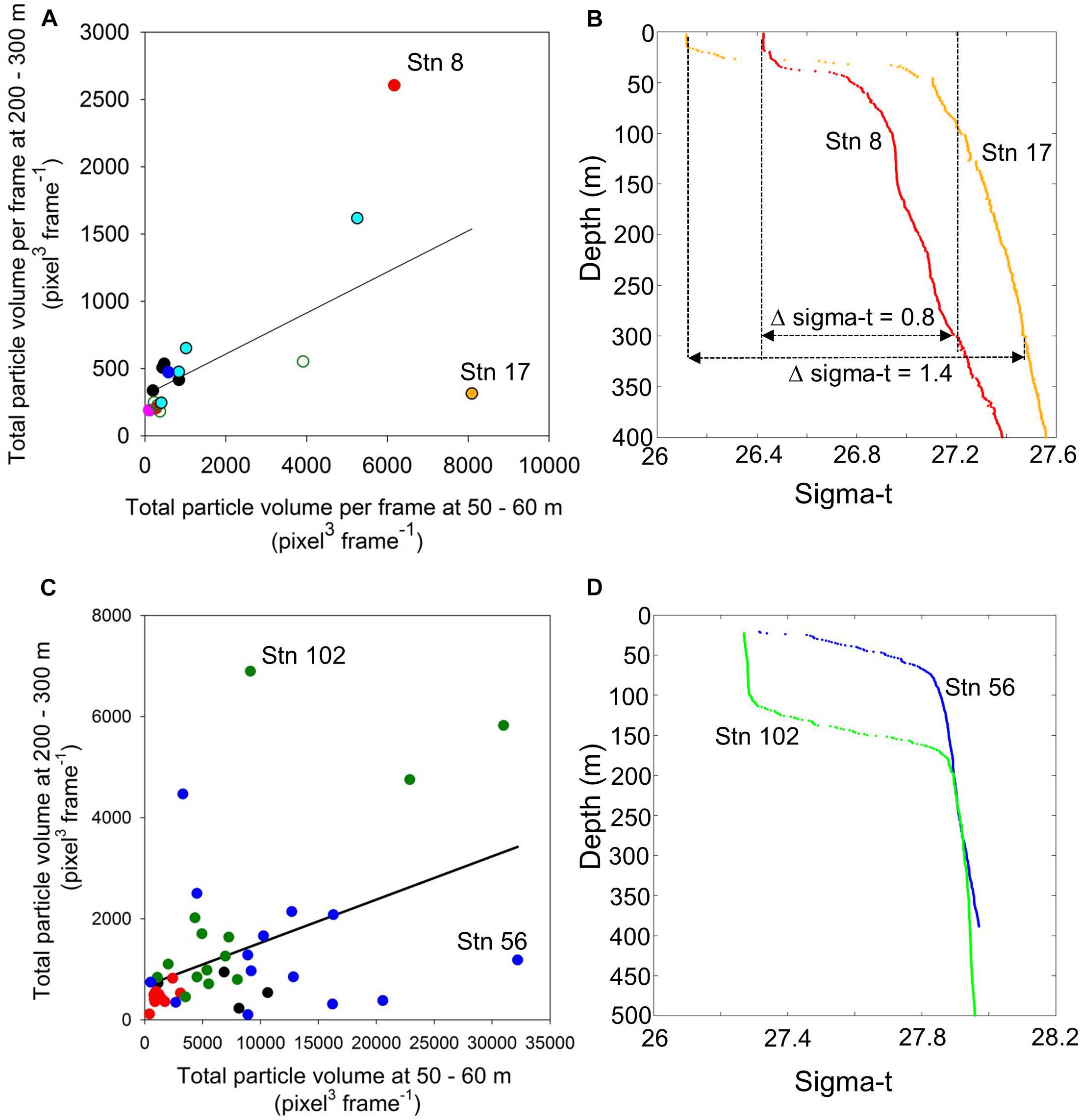
Figure 3. Mean total particle volume at 50–60 versus 200–300 m depth ranges in the North Atlantic (A) and the Ross Sea (C). The relationships between the particle inventories in the upper and lower water column were significant in both regions albeit at relatively low common variance (r²). The connectivity between particle volume abundance between upper and lower water column was highly modulated by two factors in the water column physical structure: (1) the absolute density difference (Δsigma-t) between the upper mixed layer and 300 m in the example from the North Atlantic (B), and the depth of the mixed layer in the Ross Sea (D). Color codes of data points in the North Atlantic (A): black, stations east of the Charlie Gibbs Fracture Zone (CGFZ); red, southern trench of the CGFZ; magenta, station 12 west of the CGFZ; green, northern trench of the CGFZ; orange, station 17; cyan, stations 18–21; blue, Norwegian Sea, Arctic. Color codes of data points in the Ross Sea (C): red, south site; green, Terra Nova Bay; blue, north site; black, transect stations.

While both regions (North Atlantic and Ross Sea) reflected significantly high connectivity between upper water column total volumes and those found in the deep sea, the shared variance was relatively low. The reason for this pattern can be attributed to a few stations that greatly deviated from the common slope: in the North Atlantic, stations 8 and 17 influenced the regression line in opposite directions (Figure 3A). In the Ross Sea, stations 56 and 102 represented equally extreme ends of the spectrum (Figure 3C). These apparent outliers prompted us to examine the physical structure of the water column. In the North Atlantic, station 17 had the greatest absolute density difference between the upper water column and the mesopelagic (Figure 3B). In contrast, station 8 had a density difference of almost half that value over the same depth range (Figure 3B). While there was almost no difference in absolute density of the water column between station 56 and 102 in the Ross Sea, the depth of the mixed layer was greatly increased at station 102 (Figure 3D).

Modeled export data were only available for the Ross Sea (DeJong et al., 2017). Seasonal export was significantly related to total volume at 200–300 m (Figure 4A, linear regression: n = 41, r² = 0.414, F = 27.45, p < 0.0001), significantly related to fluorescence at 200–300 m (Figure 4B, linear regression: n = 41, r² = 0.228, F = 11.50, p = 0.0018), and significantly related to the standing stock of POC at the same depth range (Figure 4C, linear regression: n = 36, r² = 0.394, F = 22.12, p < 0.0002). However, export was not significantly related to particle numbers as assessed by Coulter counts (Figure 4D, linear regression: n = 34, r² = 0.070, F = 2.398, p = 0.129). The shared variance (r²) between carbon export on the one hand, and total particle volumes at 200–300 m depth range on the other, was therefore highest, followed by POC standing stock, and fluorescence (Figure 4).

FIGURE 4

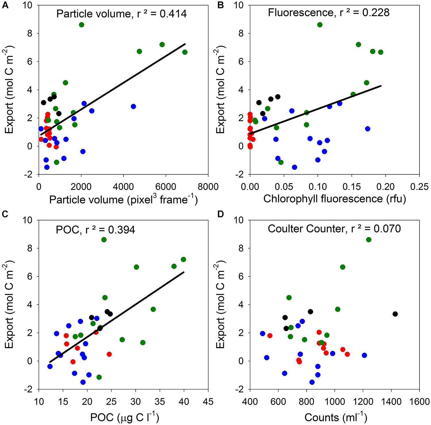
Figure 4. Seasonal export of carbon, as determined by upper water column carbon mass balance in the Ross Sea (DeJong et al., 2017), compared with mean water column particle concentrations between 200 and 300 m indicated by four different methods. (A) Total particle volume per frame determined by the video particle profiler. (B) Fluorescence measurements using a Wetlabs Fluorometer. (C) POC determined from Niskin bottle samples. (D) Coulter Counter counts for particles in the size range from 3 to 10 μm. Color codes of data points: red, south site; green, Terra Nova Bay; blue, north site; black, transect stations across the central Ross Sea (see Figure 1 for locations).

Comparing the North Atlantic and Ross Sea particle abundances, the water column of the open North Atlantic had lower average abundances than the waters of the Ross Sea shelf system. Overall, the density range was larger in the North Atlantic because of the warmer surface layer. There was a discontinuity in the density profile in the eastern stations of the North Atlantic (Figure 2A), indicative of deeper mixing likely as a result of a storm system that moved over the region during the beginning of the research expedition. This mixing could have increased the number of particles reaching deeper layers, however, in the upper water column, the particle abundance was very low at these stations under the post-spring-bloom conditions. In both regions, most of the decrease in particle abundance with depth occurred within the first 100 m (Figures 2B,D). The water column structure and absolute density values were most similar between the Arctic Ocean and the north site in the Ross Sea (Figures 2A,C).

Discussion

Connectivity of Particle Abundance Between Surface and Mesopelagic Layers

One of the fundamental assumptions for using total volumes at depth to infer exported POC rests on the connectivity between the upper ocean and the deeper layers through sinking particles. In the Ross Sea, there was indeed a highly significant correlation between particle abundance at 200–300 m and in the surface mixed layer during the same expedition, and across 77 stations sampled with the VPP (Bochdansky et al., 2017). In the North Atlantic, particle volume at 50–60 and 200–300 m was also significantly correlated albeit with high variability (Figure 3). Most interestingly, the biggest discrepancy came from two stations that had similarly high particle abundance at the surface but with drastically different abundances at depth. Both stations (8 and 17) also displayed high chlorophyll values reflecting a large standing stock of phytoplankton. Station 8 was located at the eastern entrance of the CGFZ. In this region, the subtropical and the subarctic gyres collide, creating a meandering front that leads to high primary production and export for the benefit of rich deep-water planktonic and benthic fauna (Gislason et al., 2008; Youngbluth et al., 2008; Alt et al., 2019). Station 8 had the highest surface chlorophyll values and the second highest total particle volumes at the surface, and the highest particle volumes at depth (200–300 m). While total volumes at Station 17 were even higher at the 50–60 m depth range than that of Station 8, the standing stock of particles at 200–300 m was one of the lowest during this expedition. As in the Ross Sea, water column structure appears to have had a strong effect in the connectivity between surface and deep particle inventories. Station 17 had the highest density gradient from the surface mixed layer to 300 m with a strong epipelagic pycnocline that may have acted as a physical barrier to particles reaching deeper layers (Figure 2B). Another possible explanation is that the spring bloom in that region was in a relatively early phase and that aggregation, fecal pellet production, and export had not yet begun. This scenario is less likely because of the time of year (July); standing stocks were already high at stations much further north with higher particle abundances at depth. If it was a seasonal delay (more northern stations bloom later, and the eastern Arctic blooms earlier than the western Arctic; Friedland et al., 2016), the discrepancies between surface and deep particle inventories would have been even larger at stations 18–24 but that was not the case.

Physical Water Column Characteristics and Particle Export

One of the major challenges in interpreting the role of water column stratification on particle settling velocity and export is that no single metric, such as the water column potential energy anomaly over the entire water column (Simpson and Hunter, 1974) or the locally calculated Brunt–Väisälä buoyancy frequency, adequately captures the effects of stratification on particle settling velocity and overall flux. Another problem is that the effect depends on the type of particle and whether and how fast diffusive exchange of water with the pores of the particle occurs while settling through a strong density gradient (Kindler et al., 2010; Diercks et al., 2019; and references cited therein). In all cases, however, particle velocities generally decrease in strong density gradients, forming the characteristic bands of marine snow at or just below strong pycnoclines (e.g., MacIntyre et al., 1995; Alldredge et al., 2002; Prairie et al., 2015, Prairie and White, 2017).

In the North Atlantic, stratification varied markedly among stations with a strong difference in sigma-t between stations 8 and 17 (Figure 3B). Stratification indices defined as the difference in sigma-t (Δsigma-t) between the surface and 300 m have previously been employed with a cutoff criterion between stratified and non-stratified conditions at a Δsigma-t of 0.125 kg m^–3 (Dolan et al., 2019). The depth range to reach a Δsigma-t of 0.125 kg m^–3 has also been used as the broadest definition of mixed layers in the past (de Boyer Montégut, 2004). It is noteworthy that this cutoff criterion lies between the Δsigma-t values observed at stations 8 and 17 leading to correspondingly high and low connectivity between particle abundances at the surface and depth, respectively (Figure 3B).

In the Ross Sea, differences in water column structure were the results of the depth of the mixed layer rather than absolute density differences. Due to the strong katabatic winds in TNB in the Ross Sea, especially during the second visit to the site, the main pycnocline eroded and particles were mixed deeper into the water column (Figures 2C,D, 3D). This process is similar to that previously described as the “mixed-layer pump” in the North Atlantic and in the Arctic where particles are convectively mixed deep into the water column (Gardner et al., 1995; Koeve et al., 2002; Giering et al., 2016; Wiedmann et al., 2017). Based on synchronous sediment trap and current meter observations, late summer–autumn wind-induced upper water column mixing has also been identified provoking enhanced organic C fluxes in the western Ross Sea (Langone et al., 2003). Mixing events also stimulate primary production in the surface layers due to nutrient pulses from the deep. Iron is particularly limiting in the Ross Sea, especially in the late season (e.g., Sedwick et al., 2000). A nutrient pulse due to deep mixing thus led to the high net community production we observed at TNB that late in the season (DeJong et al., 2017).

Particle Type and Export

Previous qualitative analysis of particle types at the TNB site from the same expedition revealed high abundances of heterotrophic and mixotrophic protists, diatoms such as Corethron sp., and chain-forming diatoms (Bochdansky et al., 2017). The north site had a large abundance of amorphous marine snow particles, while the south site was mostly characterized by smaller particles of unidentified composition. Consistent with previous studies (e.g., DiTullio and Smith, 1996) the transect stations in the central Ross Sea were dominated by Phaeocystis antarctica colonies (Bochdansky et al., 2017). The relationship between upper layer particle abundance and that at depth was thus very likely modulated by the particle type in addition to water column mixing as discussed above. We found only few P. antarctica colonies below 200 m as late as March 11 (Bochdansky et al., 2017), which shows that most of these colonies have not been exported yet, or resist sinking altogether (Wolf et al., 2016). In addition, P. antarctica colonies are typically not grazed by zooplankton, while the diatom-dominated TNB area very likely had associated grazers that produce fast-sinking fecal pellets. In contrast, amorphous marine snow particles that dominated the north site usually contain a large amount of gels that provide buoyancy and reduce sinking velocity (Alldredge and Crocker, 1995; Azetsu-Scott and Passow, 2004), which in turn may have kept them from sinking to the 200–300 m layer.

Total Particle Volume at Depth and Carbon Export

Carbon export determined by geochemical mass balance of carbon (DeJong et al., 2017) is an entirely independent estimate from the optically assessed total particle volume at 200–300 m. There are several caveats in estimating sinking fluxes from total particle volume at mesopelagic depths. For instance, if isopycnal transport is strong, resuspended particles can be carried far away from slopes (e.g., Gardner and Richardson, 1992; Gardner, 1997). We detected strong benthic nepheloid layers but while none of them were at 200–300 m depths (Figure 2), input from adjacent slopes may cause a problem especially in the shallow shelf systems. The other constraint is that by measuring superficial particle characteristics such as particle area, little information is available on ballast contained in particles, which is a major driver of settling velocities (e.g., Dunbar and Berger, 1981; Lima et al., 2014).

That seasonal export correlated well with several metrics of particle abundance at depth means that our timing of the research expedition in the Ross Sea was suitable to capture export. It may even be indicative that most of the carbon export occurs very late in the growing season. Late export is realistic as a delay between peak in primary production and export has previously been recorded for the Ross Sea (Dunbar et al., 1998; Sweeney et al., 2000; Langone et al., 2003) and in TNB in particular (Accornero et al., 2003). It would be interesting to investigate how well our method translates to other seasons and places, including those of relatively low export in the subtropical gyres, high export, and low particle flux attenuation with depth in the North Pacific (station K2) (Buesseler et al., 2007), or where primary production and export events are decoupled, such as in other locations of the Southern Ocean (e.g., Scotia Sea and near the Kerguelen Plateau; Maiti et al., 2013; Le Moigne et al., 2016).

Total Volume and Other Metrics of Particle Abundance

Total volume and POC behaved very similarly to estimated export. Of the three major elements of organic material (i.e., carbon, nitrogen, and phosphorus), carbon is most conserved in its transition through the water column while nitrogen and phosphorus are more rapidly remineralized, leading to increases in C:N and C:P ratios with depth (e.g., Schneider et al., 2003; Lee et al., 2004). Fluorescence is even more vulnerable to decay than N and P, which explains why fluorescence values, especially at the “south site” in the Ross Sea, were close to the detection limit (red symbols in Figure 4B), and why its relationship to estimated export is more variable than that of total volume or POC. The low explanatory power of Coulter counts for export likely had two reasons. First, Coulter counts are performed on discrete samples of very small volumes (only 0.5 ml per run × 6 runs = 3 ml per sample). In a heterogeneous environment small volume samples – by necessity – lead to high variability. Although POC measurements are also based on discrete samples collected with Niskin bottles, much larger volume (0.5–4 L depending on the depth) is used than for Coulter counts. The second, and probably more important factor, is that the size range between 3 and 10 μm in the ocean is dominated by microbes, and their abundance exponentially decreases with depth (Arístegui et al., 2009). In contrast, abundances of particles in the 100 μm to several millimeter size range either do not decrease with increasing depth, or decrease at much lower rates than the smaller size classes.

Future Directions

It is very promising that a metric as simple as total particle volume at depth is correlated to independent estimates of export based on upper-water carbon mass balance. However, total particle volume is very crude metric as it does not include particle size and morphology (Iversen et al., 2010; McDonnell and Buesseler, 2012). An important future step is the inclusion of classification of particles into sinking flux models. Smaller particles <0.1 mm can make a surprisingly high contribution to export either because of their high excess density or because of their transfer to deeper layers due to deep mixing (McDonnell and Buesseler, 2010; Giering et al., 2016). By using higher resolution images, it may also be possible to better distinguish between different particle types such as dense phytoplankton aggregates ballasted with silica shells of diatoms, marine snow buoyed by transparent polymers, highly compacted fecal pellets with high settling velocities, and carcasses of zooplankton. These classifications would likely improve particle flux estimates. Local calibrations of flux estimates of particle profiles using neutrally buoyant, free-floating gel traps (McDonnell and Buesseler, 2012) will further increase the accuracy of flux predictions. Once better classification-based calibrations are available, the high throughput of optically determined particle profilers routinely tethered to standard CTD-rosettes will allow for large-scale and frequent surveys.

Conclusion

This study shows a surprisingly robust correlation between export estimated from upper water column carbon mass balance calculations and image-based abundance of particles below the main pycnocline. This tight relationship appeared despite different time scales (one is an integrated measure, and the other a snapshot of the water column). Taking a particle census at mesopelagic depths instead of the surface also overcomes the limitations presented by a water column density structure that may not be in favor of carbon export.

Data Availability Statement

North Atlantic expedition: contextual data at http://www.microbial-oceanography.eu; Ross Sea expedition: All raw data from the VPP and the CTD context data were archived at BCO-DMO cross-listed under the name of the principal investigator (AB), and the National Science Foundation research cruise number (NBP13-02). All bottle inorganic carbon system data are available at https://www.bco-dmo.org/dataset/658394 under the name of RD (http://www.bco-dmo.org/).

Author Contributions

AB recorded the optical particle profiles, synthesized the data, and wrote the manuscript. RD contributed to the particulate carbon and carbon mass balance data, and the Ross Sea research logistics. DH contributed to the dissolved organic matter, CTD rosette context data, and research logistics for the Ross Sea expedition. GH contributed to the North Atlantic expedition logistics and the CTD rosette context data.

Funding

This research was funded by the National Science Foundation, Biological Oceanography (Awards #0826659 and #1851368 to AB), Austrian Science Fund (FWF) project 1486-B09 (GH), the European Research Council under the European Community’s Seventh Framework Program (FP7/2007-2013) ERC Grant Agreement No. 268595 (MEDEA project) to GH, and the National Science Foundation, Ocean Polar Program: NSF/OPP Awards #1142097 (AB), #1142044 (RD), and #1142117 (DH).

Conflict of Interest

The authors declare that the research was conducted in the absence of any commercial or financial relationships that could be construed as a potential conflict of interest.

Acknowledgments

We thank the crews of the RV Pelagia and RVIB Nathaniel B. Palmer. Cody E. Garrison (ODU) and Melissa A. Clouse (ODU) operated the Coulter counter. Christopher MacGregor (Cybermato Consulting, Seattle, WA, United States) modified the Avidemux software for particle analysis.

Supplementary Material

The Supplementary Material for this article can be found online at: https://www.frontiersin.org/articles/10.3389/fmars.2019.00778/full#supplementary-material

References

Accornero, A., Manno, C., Esposito, F., and Gambi, M. (2003). The vertical flux of particulate matter in the polynya of Terra Nova Bay. Part II. Biol. Comp. Antarc. Sci. 15, 175–188. doi: 10.1017/S0954102003001214

CrossRef Full Text | Google Scholar

Alldredge, A. L., Cowles, T. J., MacIntyre, S., Rines, J. E. B., Donaghay, P. L., Greenlaw, C. F., et al. (2002). Occurrence and mechanisms of formation of a dramatic thin layer of marine snow in a shallow Pacific fjord. Mar. Ecol. Prog. Ser. 233, 1–12. doi: 10.3354/meps233001

CrossRef Full Text | Google Scholar

Alldredge, A. L., and Crocker, K. M. (1995). Why do sinking mucilage aggregates accumulate in the water column? Sci. Total Environ. 165, 15–22. doi: 10.1016/0048-9697(95)04539-D

CrossRef Full Text | Google Scholar

Alt, C. H. S., Kremenetskaia, A., Gebruk, A. V., Gooday, A. J., and Jones, D. O. B. (2019). Bathyal benthic megafauna from the Mid-Atlantic Ridge in the region of the Charlie-Gibbs fracture zone based on remotely operated vehicle observations. Deep-Sea Res. Part I 145, 1–12. doi: 10.1016/j.dsr.2018.12.006

CrossRef Full Text | Google Scholar

Arístegui, J., Gasol, J. M., Duarte, C. M., and Herndl, G. J. (2009). Microbial oceanography of the dark ocean’s pelagic realm. Limnol. Oceanogr. 54, 1501–1529. doi: 10.4319/lo.2009.54.5.1501

CrossRef Full Text | Google Scholar

Arrigo, K. R., Robinson, D. H., Worthen, D. L., Dunbar, R. B., DiTullio, G. R., VanWoert, M., and Lizotte, M. P. (1999). Phytoplankton community structure and the drawdown of nutrients and CO2 in the southern ocean. Science 283, 365–367. doi: 10.1126/science.283.5400.365

PubMed Abstract | CrossRef Full Text | Google Scholar

Asper, V. L. (1987). Measuring the flux and sinking speed of marine snow aggregates. Deep Sea Res. Part A 34, 1–17. doi: 10.1016/0198-0149(87)90117-8

CrossRef Full Text | Google Scholar

Azetsu-Scott, K., and Passow, U. (2004). Ascending marine particles: significance of transparent exopolymer particles (TEP) in the upper ocean. Limnol. Oceanogr. 49, 741–748. doi: 10.4319/lo.2004.49.3.0741

CrossRef Full Text | Google Scholar

Bochdansky, A. B., Clouse, M. A., and Herndl, G. J. (2016). Dragon kings of the deep sea: marine particles deviate markedly from the common number-size spectrum. Sci. Rep. 6:22633. doi: 10.1038/srep22633

PubMed Abstract | CrossRef Full Text | Google Scholar

Bochdansky, A. B., Clouse, M. A., and Hansell, D. A. (2017). Mesoscale and high-frequency variability of macroscopic particles (> 100 μm) in the Ross Sea and its relevance for late-season particulate carbon export. J. Mar. Syst. 166, 120–131. doi: 10.1016/j.jmarsys.2016.08.010

CrossRef Full Text | Google Scholar

Bochdansky, A. B., Jericho, M. H., and Herndl, G. J. (2013). Development and deployment of a point-source digital inline holographic microscope for the study of plankton and particles to a depth of 6000 m: deep-sea holographic microscopy. Limnol. Oceanogr. 11, 28–40. doi: 10.4319/lom.2013.11.28

CrossRef Full Text | Google Scholar

Buesseler, K. O., and Boyd, P. W. (2009). Shedding light on processes that control particle export and flux attenuation in the twilight zone of the open ocean. Limnol. Oceanogr. 54, 1210–1232. doi: 10.4319/lo.2009.54.4.1210

CrossRef Full Text | Google Scholar

Buesseler, K. O., Lamborg, C. H., Boyd, P. W., Lam, P. J., Trull, T. W., Bidigare, R. R., et al. (2007). revisiting carbon flux through the ocean’s twilight zone. Science 316, 567–570. doi: 10.1126/science.1137959

PubMed Abstract | CrossRef Full Text | Google Scholar

Carlson, C. A., Hansell, D. A., Peltzer, E. T., and Smith, W. O. (2000). Stocks and dynamics of dissolved and particulate organic matter in the southern Ross Sea. Antarctica. Deep Sea Res. Part II 47, 3201–3225. doi: 10.1016/S0967-0645(00)00065-5

CrossRef Full Text | Google Scholar

Cowen, R. K., and Guigand, C. M. (2008). In situ ichthyoplankton imaging system (I SIIS): system design and preliminary results: in situ ichthyoplankton imaging system. Limnol. Oceanogr. 6, 126–132. doi: 10.4319/lom.2008.6.126

CrossRef Full Text | Google Scholar

de Boyer Montégut, C. (2004). Mixed layer depth over the global ocean: an examination of profile data and a profile-based climatology. J. Geophys. Res. 109:C12003. doi: 10.1029/2004JC002378

CrossRef Full Text | Google Scholar

DeJong, H. B., Dunbar, R. B., Koweek, D. A., Mucciarone, D. A., Bercovici, S. K., and Hansell, D. A. (2017). Net community production and carbon export during the late summer in the Ross Sea. Antarctica: late summer NCP in the Ross Sea. Glob. Biogeochem. Cycles 31, 473–491. doi: 10.1002/2016GB005417

CrossRef Full Text | Google Scholar

Dickson, A. G., Sabine, C. L., and Christian, J. R. (2007). “Guide to best practices for ocean CO₂ measurements,” in PICES Special Publication;3 IOCCP Report; 8, Sydney: North Pacific Marine Science Organization).

Google Scholar

Diercks, A., Ziervogel, K., Sibert, R., Joye, S. B., Asper, V., and Montoya, J. P. (2019). Vertical marine snow distribution in the stratified, hypersaline, and anoxic Orca Basin (Gulf of Mexico). Elem. Sci. Anth. 7:10. doi: 10.1525/elementa.348

CrossRef Full Text | Google Scholar

DiTullio, G. R., and Smith, W. O. (1996). Spatial patterns in phytoplankton biomass and pigment distributions in the Ross Sea. J. Geophys. Res. 101, 18467–18477. doi: 10.1029/96JC00034

CrossRef Full Text | Google Scholar

Dolan, J. R., Ciobanu, M., Marro, S., and Coppola, L. (2019). An exploratory study of heterotrophic protists of the mesopelagic Mediterranean Sea. ICES J. Mar. Sci. 76, 616–625. doi: 10.1093/icesjms/fsx218

CrossRef Full Text | Google Scholar

Dunbar, B. R., and Berger, H. W. (1981). Fecal pellet flux to modern bottom sediment of Santa Barbara Basin (California) based on sediment trapping. Geol. Soc. Am. Bull. 92:212. doi: 10.1130/0016-7606(1981)92<212:fpftmb>2.0.co;2

CrossRef Full Text | Google Scholar

Dunbar, R. B., Leventer, A. R., and Mucciarone, D. A. (1998). Water column sediment fluxes in the Ross Sea. Antarctica: atmospheric and sea ice forcing. J. Geophys. Res. 103, 30741–30759. doi: 10.1029/1998JC900001

CrossRef Full Text | Google Scholar

Estapa, M., Durkin, C., Buesseler, K., Johnson, R., and Feen, M. (2017). Carbon flux from bio-optical profiling floats: calibrating transmissometers for use as optical sediment traps. Deep Sea Res. Part I 120, 100–111. doi: 10.1016/j.dsr.2016.12.003

CrossRef Full Text | Google Scholar

Friedland, K. D., Record, N. R., Asch, R. G., Kristiansen, T., Saba, V. S., Drinkwater, K. F., et al. (2016). Seasonal phytoplankton blooms in the North Atlantic linked to the overwintering strategies of copepods. Elementa 4:000099. doi: 10.12952/journal.elementa.000099

CrossRef Full Text | Google Scholar

Gardner, W. (1997). The flux of particles to the deep sea: methods, measurements, and mechanisms. Oceanography 10, 116–121. doi: 10.5670/oceanog.1997.03

CrossRef Full Text | Google Scholar

Gardner, W. D., Chung, S. P., Richardson, M. J., and Walsh, I. D. (1995). The oceanic mixed-layer pump. Deep Sea Res. Part II 42, 757–775. doi: 10.1016/0967-0645(95)00037-Q

CrossRef Full Text | Google Scholar

Gardner, W. D., and Richardson, M. J. (1992). “Particle export and resuspension fluxes in the western north atlantic,” in Deep-Sea Food Chains and the Global Carbon Cycle, eds G. T. Rowe, and V. Pariente, (Dordrecht: Springer Netherlands), 339–364. doi: 10.1007/978-94-011-2452-2_21

CrossRef Full Text | Google Scholar

Giering, S. L. C., Richard, S., Martin, A. P., Henson, S. A., Riley, J. S., and Marsay, C. M. (2017). Particle flux in the oceans: challenging the steady state assumption. Glob. Biogeochem. Cycles 31, 159–171. doi: 10.1002/2016gb005424

CrossRef Full Text | Google Scholar

Giering, S. L. C., Sanders, R., Martin, A. P., Lindemann, C., Möller, K. O., Daniels, C. J., et al. (2016). High export via small particles before the onset of the North Atlantic spring bloom: small particle export before the bloom. J. Geophys. Res. 121, 6929–6945. doi: 10.1002/2016JC012048

CrossRef Full Text | Google Scholar

Gislason, A., Gaard, E., Debes, H., and Falkenhaug, T. (2008). Abundance, feeding and reproduction of Calanus finmarchicus in the Irminger Sea and on the northern Mid-Atlantic Ridge in June. Deep-Sea Res. Part II 2, 72–82. doi: 10.1016/j.dsr2.2007.09.008

CrossRef Full Text | Google Scholar

Guidi, L., Jackson, G. A., Stemmann, L., Miquel, J. C., Picheral, M., and Gorsky, G. (2008). Relationship between particle size distribution and flux in the mesopelagic zone. Deep Sea Res. Part I 55, 1364–1374. doi: 10.1016/j.dsr.2008.05.014

CrossRef Full Text | Google Scholar

Iversen, M. H., Nowald, N., Ploug, H., Jackson, G. A., and Fischer, G. (2010). High resolution profiles of vertical particulate organic matter export off Cape Blanc. Mauritania: degradation processes and ballasting effects. Deep Sea Res. Part I 57, 771–784. doi: 10.1016/j.dsr.2010.03.007

CrossRef Full Text | Google Scholar

Jackson, G. A., Maffione, R., David, K., Costello, D. K., Alice, L., Alldredge, A. L., et al. (1997). Particle size spectra between 1 um and 1 cm at Monterey Bay determined using multiple instruments. Deep-Sea Res. I 44, 1739–1767. doi: 10.1016/S0967-0637(97)00029-0

CrossRef Full Text | Google Scholar

Kindler, K., Khalili, A., and Stocker, R. (2010). Diffusion-limited retention of porous particles at density interfaces. Proc. Natl. Acad. Sci. U.S.A. 107, 22163–22168. doi: 10.1073/pnas.1012319108

PubMed Abstract | CrossRef Full Text | Google Scholar

Koeve, W., Pollehne, F., Oschlies, A., and Zeitzschel, B. (2002). Storm-induced convective export of organic matter during spring in the northeast Atlantic Ocean. Deep Sea Res. Part I 49, 1431–1444. doi: 10.1016/S0967-0637(02)00022-5

CrossRef Full Text | Google Scholar

Langone, L., Dunbar, R. B., Mucciarone, D. A., Ravaioli, M., Meloni, R., and Nittrouer, C. A. (2003). “), Rapid sinking of biogenic material during the late austral summer in the Ross Sea, Antarctica,” in Biogeochemistry of the Ross Sea, Vol. 78, eds G. DiTullio, and R. Dunbar, (Washington, D.C: American Geophysical Union), 221–234.

Google Scholar

Le Moigne, F. A. C., Henson, S. A., Cavan, E., Georges, C., Pabortsava, K., Achterberg, E. P., et al. (2016). What causes the inverse relationship between primary production and export efficiency in the Southern Ocean?: PP and e Ratio in the Southern Ocean. Geophys. Res. Lett. 43, 4457–4466. doi: 10.1002/2016GL068480

CrossRef Full Text | Google Scholar

Lee, C., Wakeham, S., and Arnosti, C. (2004). Particulate organic matter in the sea: the composition conundrum. AMBIO 33, 565–575. doi: 10.1579/0044-7447-33.8.565

PubMed Abstract | CrossRef Full Text | Google Scholar

Lemaitre, N., Planchon, F., Planquette, H., Dehairs, F., Fonseca-Batista, D., Roukaerts, A., et al. (2018). High variability of particulate organic carbon export along the North Atlantic GEOTRACES section GA01 as deduced from ²³⁴Th fluxes. Biogeosciences 15, 6417–6437. doi: 10.5194/bg-15-6417-2018

CrossRef Full Text | Google Scholar

Lima, I. D., Lam, P. J., and Doney, S. C. (2014). Dynamics of particulate organic carbon flux in a global ocean model. Biogeosciences 11, 1177–1198. doi: 10.5194/bg-11-1177-2014

PubMed Abstract | CrossRef Full Text | Google Scholar

Lindensmith, C. A., Rider, S., Bedrossian, M., Wallace, J. K., Serabyn, E., Showalter, G. M., et al. (2016). A Submersible, off-axis holographic microscope for detection of microbial motility and morphology in aqueous and icy environments. PLoS One 11:e0147700. doi: 10.1371/journal.pone.0147700

PubMed Abstract | CrossRef Full Text | Google Scholar

Long, M. C., Dunbar, R. B., Tortell, P. D., Smith, W. O., Mucciarone, D. A., and DiTullio, G. R. (2011). Vertical structure, seasonal drawdown, and net community production in the Ross Sea. Antarctica. J. Geophys. Res. 116:C10029. doi: 10.1029/2009JC005954

CrossRef Full Text | Google Scholar

Luo, J. Y., Irisson, J.-O., Graham, B., Guigand, C., Sarafraz, A., Mader, C., et al. (2018). Automated plankton image analysis using convolutional neural networks: automated plankton image analysis using CNNs. Limnol. Oceanogr. 16, 814–827. doi: 10.1002/lom3.10285

CrossRef Full Text | Google Scholar

MacIntyre, S., Alldredge, A. L., and Gotschalk, C. C. (1995). Accumulation of marines now at density discontinuities in the water column. Limnol. Oceanogr. 40, 449–468. doi: 10.4319/lo.1995.40.3.0449

CrossRef Full Text | Google Scholar

Maiti, K., Charette, M. A., Buesseler, K. O., and Kahru, M. (2013). An inverse relationship between production and export efficiency in the Southern Ocean: export efficiency in the Southern. Geophys. Res. Lett. 40, 1557–1561. doi: 10.1002/grl.50219

CrossRef Full Text | Google Scholar

Malkiel, E., Alquaddoomi, O., and Katz, J. (1999). Measurements of plankton distribution in the ocean using submersible holography. Measure. Sci. Technol. 10, 1142–1152.

Google Scholar

Manly, B. F. J. (2007). Randomization, Bootstrap and Monte Carlo Methods in Biology. Third Edition. Boca Raton: Chapman & Hall/CRC.

Google Scholar

McDonnell, A. M. P., and Buesseler, K. O. (2010). Variability in the average sinking velocity of marine particles. Limnol. Oceanogr. 55, 2085–2096. doi: 10.4319/lo.2010.55.5.2085

CrossRef Full Text | Google Scholar

McDonnell, A. M. P., and Buesseler, K. O. (2012). A new method for the estimation of sinking particle fluxes from measurements of the particle size distribution, average sinking velocity, and carbon content: estimation of sinking particle fluxes. Limnol. Oceanogr. 10, 329–346. doi: 10.4319/lom.2012.10.329

CrossRef Full Text | Google Scholar

McGill, P. R., Henthorn, R. G., Bird, L. E., Huffard, C. L., Klimov, D. V., and Smith, K. L. Jr. (2016). Sedimentation event sensor: new ocean instrument for in situ imaging and fluorometry of sinking particulate matter. Limnol. Oceanogr. Methods 14, 853–863. doi: 10.1002/lom3.10131

CrossRef Full Text | Google Scholar

Ohman, M. D., Davis, R. E., Sherman, J. T., Grindley, K. R., Whitmore, B. M., Nickels, C. F., et al. (2019). Zooglider: an autonomous vehicle for optical and acoustic sensing of zooplankton: autonomous Zooglider. Limnol. Oceanogr. 17, 69–86. doi: 10.1002/lom3.10301

CrossRef Full Text | Google Scholar

Orsi, A., Smethie, W., and Bullister, J. (2002). On the total input of Antarctic waters to the deep ocean: a preliminary estimate from chlorofluorocarbon measurements. J. Geophys. Res 107:3122. doi: 10.1029/2001JC000976

CrossRef Full Text | Google Scholar

Prairie, J. C., and White, B. L. (2017). A model for thin layer formation by delayed particle settling at sharp density gradients. Continent. Shelf Res. 133, 37–46. doi: 10.1016/j.csr.2016.12.007

CrossRef Full Text | Google Scholar

Prairie, J. C., Ziervogel, K., Camassa, R., McLaughlin, R. M., White, B. L., Dewald, C., et al. (2015). Delayed settling of marine snow: effects of density gradient and particle properties and implications for carbon cycling. Mar. Chem. 175, 28–38. doi: 10.1016/j.marchem.2015.04.006

CrossRef Full Text | Google Scholar

Sanders, R., Henson, S. A., Koski, M., De La Rocha, C. L., Painter, S. C., Poulton, A. J., et al. (2014). The biological carbon pump in the North Atlantic. Prog. Oceanogr. 129, 200–218. doi: 10.1016/j.pocean.2014.05.005

CrossRef Full Text | Google Scholar

Schlitzer, R. (2018). Ocean Data View, odv.awi.de, 2018^∗.

Google Scholar

Schneider, B., Schlitzer, R., Fischer, G., and Nöthig, E.-M. (2003). Depth-dependent elemental compositions of particulate organic matter (POM) in the ocean: depth-dependent c:n ratios of pom in the ocean. Glob. Biogeochem. Cycles 17:1032. doi: 10.1029/2002GB001871

CrossRef Full Text | Google Scholar

Sedwick, P. N., DiTullio, G. R., and Mackey, D. J. (2000). Iron and manganese in the Ross Sea, Antarctica: seasonal iron limitation in Antarctic shelf waters. J. Geophys. Res. 105, 11321–11336. doi: 10.1029/2000JC000256

CrossRef Full Text | Google Scholar

Simpson, J. H., and Hunter, J. R. (1974). Fronts in the Irish Sea. Nature 250, 404–406. doi: 10.1038/250404a0

CrossRef Full Text | Google Scholar

Smith, W. O., Tozzi, S., Long, M. C., Sedwick, P. N., Peloquin, J. A., Dunbar, R. B., et al. (2013). Spatial and temporal variations in variable fluoresence in the Ross Sea (Antarctica): oceanographic correlates and bloom dynamics. Deep Sea Res. Part I 79, 141–155. doi: 10.1016/j.dsr.2013.05.002

CrossRef Full Text | Google Scholar

Stemmann, L., Jackson, G. A., and Ianson, D. (2004). A vertical model of particle size distributions and fluxes in the midwater column that includes biological and physical processes—Part I: model formulation. Deep Sea Res. Part I 51, 865–884. doi: 10.1016/j.dsr.2004.03.001

CrossRef Full Text | Google Scholar

Sweeney, C., Hansell, D. A., Carlson, C. A., Codispoti, L., Gordon, L. I., Marra, J., et al. (2000). Biogeochemical regimes, net community production and carbon export in the Ross Sea. Antarctica. Deep Sea Res. Part II 47, 3369–3394. doi: 10.1016/S0967-0645(00)00072-2

CrossRef Full Text | Google Scholar

Valdes, J. R., and Price, J. F. (2000). A neutrally buoyant, upper ocean sediment trap. J. Atmos. Oceanic Technol. 17, 62–68. doi: 10.1175/1520-0426(2000)017<0062:anbuos>2.0.co;2

CrossRef Full Text | Google Scholar

Walsh, I. D., and Gardner, W. D. (1992). A comparison of aggregate profiles with sediment trap fluxes. Deep Sea Res. Part A 39, 1817–1834. doi: 10.1016/0198-0149(92)90001-A

CrossRef Full Text | Google Scholar

Watson, J., Alexander, S., Craig, G., Hendry, D. C., Hobson, P. R., Lampitt, R. S., et al. (2001). Simultaneous in-line and off-axis subsea holographic recording of plankton and other marine particles. Measure. Sci. Technol. 12, L9–L15. doi: 10.1088/0957-0233/12/8/101

CrossRef Full Text | Google Scholar

Wiedmann, I., Tremblay, J. -É, Sundfjord, A., and Reigstad, M. (2017). Upward nitrate flux and downward particulate organic carbon flux under contrasting situations of stratification and turbulent mixing in an Arctic shelf sea. Elem. Sci. Anth. 5: 43. doi: 10.1525/elementa.235

CrossRef Full Text | Google Scholar

Wolf, C., Iversen, M., Klaas, C., and Metfies, K. (2016). Limited sinking of Phaeocystis during a 12 days sediment trap study. Mol. Ecol. 25, 3428–3435. doi: 10.1111/mec.13697

PubMed Abstract | CrossRef Full Text | Google Scholar

Xu, W., Jericho, M. H., Meinertzhagen, I. A., and Kreuzer, H. J. (2001). Digital in-line holography for biological applications. Proc. Natl. Acad. Sci. U.S.A. 98, 11301–11305. doi: 10.1073/pnas.191361398

PubMed Abstract | CrossRef Full Text | Google Scholar

Youngbluth, M., Sørnes, T., Hosia, A., and Stemmann, L. (2008). Vertical distribution and relative abundance of gelatinous zooplankton, in situ observations near the Mid-Atlantic Ridge. Deep-Sea Res. Part II 55, 119–125. doi: 10.1016/j.dsr2.2007.10.002

CrossRef Full Text | Google Scholar

Zheng, H., Wang, R., Yu, Z., Wang, N., Gu, Z., and Zheng, B. (2017). Automatic plankton image classification combining multiple view features via multiple kernel learning. BMC Bioinformatics 18:570. doi: 10.1186/s12859-017-1954-8

PubMed Abstract | CrossRef Full Text | Google Scholar