Sensitivity of a 3D Shelf Sea Ecosystem Model to Parameterizations of the Underwater Light Field

1. Introduction

A common class of biological models are the Nutrient, Zooplankton, Phytoplankton and Detritus (NPZD) models, which are usually simple four component models. Other models are immensely more complex with several, in some cases uncoupled nutrient cycles, functional groups of phyto- and zooplankton, bacteria, etc. (e.g., Fasham et al., 1990; Baretta et al., 1995; Kühn and Radach, 1997; Moll, 1997, 1998; Bissett et al., 1999, 2001; Chai et al., 2002; Schrum et al., 2006a,b; Daewel and Schrum, 2013). What all of these models have in common, however, is that for phytoplankton growth, specifically for photosynthesis, light is required.

There are various approaches to treat light in biological models. Especially in the early years of ecosystem modeling, simplifications had to be made due to the limitations in affordable computational power. Common approximations that are found in literature are spacially averaging the physics (Baretta et al., 1995; Lenhart et al., 1995; Chai et al., 2002), or using spectrally integrated irradiance or photosynthetically available radiation (PAR) instead of a spectral approach (Baretta et al., 1995; Chai et al., 2002; Schrum et al., 2006a; Daewel and Schrum, 2013). For some purposes, a simple approach may well be appropriate. However, Mobley et al. (2015) have shown that both a spectral light treatment and the inclusion of a daily cycle can significantly change the results of a biological model, while technological advances have made these approaches more affordable. Thus, for quantitatively more correct, complex and precise applications, it is advisable to use fewer approximations. In our case, the sparsity of available spectral data, the greater effort in evaluating a spectral model, justify the use of spectrally integrated irradiance.

In many biological models, attenuation due to suspended particulate matter (SPM) is sometimes considered indirectly by increasing the attenuation coefficient of water, which is often assumed constant in space and time. Hence, such approaches only show spacial or temporal variability of light attenuation due to chlorophyll, yet not due to SPM. However, many areas of the North Sea are rich in SPM and independently so of chlorophyll, with rather high horizontal variability (e.g., van der Molen et al., 2009). An online coupling between the optical components of a biogeochemical and the physical model is rare, however, it has been shown that optically active water constituents can influence the physics significantly (Cahill et al., 2008; Mobley et al., 2015). Cahill et al. (2008) found feedback mechanisms between light attenuation and the resulting mixed layer depth. They concluded that stronger stratification leads to higher concentrations of optically active water components in the upper water column, causing the stratification to become even stronger. This indicates the importance of considering vertical variability of attenuation. However, many models do not consider horizontally or vertically varying turbidity.

The light climate in the North Sea has been subject to change over the past decades. Recent studies on Secchi-depth data have found centennial negative trends, indicating an increase in turbidity and a subsequent decrease in light availability for photosynthesis (Dupont and Aksnes, 2013; Capuzzo et al., 2015). Capuzzo et al. (2015) defined distinct areas through their hydrodynamic properties as permanently mixed, seasonally stratified, intermediate, regions of fresh water influence and the East Anglia plume. They attributed significant decreases in mean Secchi-depths from the first to the second half of the twentieth century to SPM (e.g., due to increased dredging) and chlorophyll (Capuzzo et al., 2015) or colored dissolved organic matter (CDOM) (Dupont and Aksnes, 2013). Both SPM and CDOM have been found to have a stronger effect on light attenuation than chlorophyll has (Harvey et al., 2019). Opdal et al. (2019) support the hypothesis that the coastal darkening is not impacted by changes in chlorophyll, but rather non-planktonic substances, i.e., SPM and CDOM. The darkening has been shown to delay the spring bloom of phytoplankton (Opdal et al., 2019). Wilson and Heath (2019) indicate that over the past 20 years, due to climate change and a subsequent change in the wind regime, the trends of increasing SPM over the twentieth century might have reversed in several areas of the North Sea. The above mentioned works motivate investigations into how changes to the light climate affect the ecosystem in the North Sea, given the apparent trend in reduced light availability and increased turbidity, especially in the southern North Sea.

We aim to analyse the underwater light field numerically, and specifically the effects of introducing heterogeneous, bathymetry dependent turbidity. For this purpose, we set up a three-dimensional (3D) hydrodynamic model (ROMS), coupled with a one-dimensional (1D) biological model (CoSiNE) of the North Sea. We modified the classic light treatment in CoSiNE, making the attenuation effectively bathymetry dependent and vertically increasing, independently of phytoplankton. This is to accommodate for the greater turbidity in shallow coastal waters, while being virtually no more expensive in terms of computational effort than the original formulation. We test the capability of the modified light treatment as a functioning proxy for attenuation due to horizontally varying inorganic SPM. For reasons of simplicity, we exclude both the effects of CDOM and temporal changes in SPM in this work.

Through sensitivity studies, the impact of reduced light availability is determined. The model results are compared to the Atlantic Margin Model with 7 km horizontal resolution of the MetOffice, UK, and the European Regional Seas Ecosystem Model (ERSEM, Baretta et al., 1995; Blackford et al., 2004), to which AMM7 is coupled, using the reanalyzed data as provided by the Copernicus Marine Environment Monitoring Service (CMEMS, http://marine.copernicus.eu), Chlorophyll Color Index (CCI, https://esa-oceancolour-cci.org) satellite data, as well as bottle and FerryBox data, provided by the International Council for Exploration of the Sea (ICES, https://ices.dk) and the Coastal Observing System for Northern and Arctic Seas (COSYNA, https://www.hzg.de/institutes_platforms/cosyna/index.php.de, Baschek et al., 2017), respectively. The models, the used data and the experiments are described in section 2. The results are described and discussed in section 3, and the conclusions we draw from them are found in section 4. A brief overview of the model's physical performance can be found in the supplement.

2. Data and Methods

2.1. Physical Model

The physical model is the regional ocean modeling system (ROMS) (Haidvogel et al., 2000). It solves the primitive equations, using a split-explicit time-stepping scheme. In the vertical, it utilizes a terrain-following s-coordinate (Song and Haidvogel, 1994), and in the horizontal a curvilinear structured grid. Turbulence closure is achieved with a generic length scale (GLS) approach in a k-kl configuration (Umlauf and Burchard, 2003; Warner et al., 2005).

The horizontal grid is taken from the MetOffice's AMM7 model, as is available from the COPERNICUS web portal, extended from 5°W to 13°E and 48°N to 60°N. The horizontal resolution is 7 km. In the vertical, the domain is divided into 35 s-layers, stretched to increase the resolution at the surface. The initial and boundary conditions (IC and BC) were taken from AMM7 as well. We applied a Champman type BC for the free surface, which is tidally filtered and averaged daily and the ROMS tidal constituent model using Finite Element Solution (FES, the 2014 model as provided by AVISO) tides, contributing the tidal signal. A Flather type BC was chosen for 2D-momentum, and radiation with nudging BC for 3D-momentum and tracers. The atmospheric forcing is taken from NCEP/NCAR and is of a quarter daily temporal and 21 km horizontal resolution. The river input is climatological, and is taken from the pan-European Hydrological Predictions for the Environment (E-HYPE) model of the Swedish Meteorological and Hydrological Institute (SMHI), which gives freshwater fluxes from 34 rivers discharging into the Baltic Sea and North Sea. For reasons of simplicity, we have used only the rivers Trent, Thames, Seinne, Maas, Rhine, Schelde, Ems, Weser, Elbe, and Glomma, as well as the combined outflow of the Baltic Sea in the Kattegat.

The vertical coordinate in ROMS can be configured in such a way that all surface layers are at the same approximate geopotential depth. This is beneficial for reducing pressure gradient error and other density related issues that s-coordinates typically have. Our model has strong horizontal density gradients in several areas of the domain, e.g., the German Bight or the Skagerrak. While the German Bight is relatively shallow and has comparably smooth bathymetry gradients, the same cannot be said about the Skagerrak. The errors resulting from using conventional s-coordinates, where the surface layers are not at approximately the same geopotential depths, are thus expected to be relatively small in the German Bight, and larger in the Skagerrak. Therefore, a detailed comparison to the output of AMM7 has been performed. Our simulations are satisfactorily similar to that of AMM7 (not shown). We describe in section 2.3.2 that our light parameterization benefits from our model's surface layers not being equally distributed.

2.2. Biological Model

The biological model is the CoSiNE model, as developed by Chai et al. (2002). In the used version, it consists of 11 state variables, including the four nutrients nitrate (NO3), ammonium (NH4), silicate (SiOH4), and phosphate (PO4), two phytoplankton groups (small phytoplankton, S1 and diatoms, S2), two zooplankton groups (microzooplankton, Z1 and mesozooplankton, Z2), as well as detrital nitrogen (dN) and silicate (dS), as well as oxygen (O2). All plankton groups are expressed in units of mmol N m⁻³. The details may be found e.g., in Chai et al. (2002) and Liu et al. (2018). Nitrate uptake by phytoplankton may be inhibited, if ammonium is more abundant than nitrate (Liu et al., 2018), however, we do not make use of this function. The biological IC and BC (in the 3D-model) are taken from AMM7-ERSEM, as available from CMEMS (described in section 2.4). In the case of those variables that arent available, typical ratios are assumed, e.g., ammonium is assumed to be of about a tenth the abundance of nitrate. Plankton BC are of Neumann type. River input of nutrients is taken from E-HYPE.

2.3. Light Parameterization

2.3.1. Classic Formulation

The exponential decay of irradiance (e.g., Evans and Parslow, 1985; Zielinski et al., 2002) is perhaps the most frequently used formulation of light in biological models. The basis of this scheme can be found in the description of CoSiNE (Chai et al., 2002), with additions regarding SPM made in recent works (Liu et al., 2018).

$\begin{array}{ll}I\left(z\right)=I_0.\text{ exp}\left(cff1\right))& (1)\end{array}$

$\begin{array}{l}cff1=a_w·(\zeta -z)+a_p{\displaystyle {\int }_z^{\zeta }}(P1+P2)\text{ d}{z}^{\prime }\\ +{\displaystyle {\int }_z^{\zeta }}{a}_{SPM}SPM\text{ d}{z}^{\prime },& (2)\end{array}$

with ζ being the free surface height, and a_w = 0.036 1/m, $a_p=0.03m^2/mmolN$ and a_SPM being the attenuation coefficients, specifically for water, phytoplankton and inorganic SPM. P1 and P2 are the phytoplankton biomass of small phytoplankton and diatoms, respectively, in units of mmol N/m³, taken from CoSiNE. Because there is a technical possibility to compute SPM, it is included in Equation (2). It is, however, excluded in the experiment, because SPM content is not known, so that it cannot be explicitly prescribed and we do not couple our model to a sediment and wind wave module. A homogeneous approach is not valid for the entire domain, due to the large horizontal variability, and a vertical distribution function would need to be found and validated first.

2.3.2. Index Scheme

The index (IND) scheme was designed as a cost efficient way to estimate the effects of SPM on light attenuation, by multiplying the right hand side of Equation (2) with a factor k/N, where k ∈ [1, 2, 3, …, N] is the layer index and N is the total number of layers, k = 1 being the bottom most layer and k = N being the top layer. This way, the attenuation is strongest at the bottom. While in the classic scheme, the 1%-depth is exactly twice the 10%-depth, in the IND scheme, this is not the case. Figure B.1A shows the ratio of 1%-depth over 10%-depth in the default state (without chlorophyll specific attenuation). Note that it is slightly larger than 2 in the deeper areas, but slightly smaller than 2 elsewhere. This is due to the stretching of the vertical coordinate (see section 2.1). The full modified version of Equations (1) and (2) then reads

$\begin{array}{l}{I}_{IND}\left(z\right)=I_0·k/N·exp\left(-a_{w}z-a_p{\displaystyle {\int }_z^{\zeta }}\left(P1+P2\right)\text{ d}z\right)\\ =I_{classic}\left(z\right)·k/N,& (3)\end{array}$

with k/N taking the role of $exp\left(-a_{SPM}{\int }_z^{\zeta }SMP\text{d}z\right)$. Because k/N ≤ 1, downwelling irradiance is always lower in the IND scheme below the top most layer.

There are mathematical and physical inconsistencies in this formulation. Taking the factor k/N into the exponential, and discretizing yields

$\begin{array}{l}I\left(z_k\right)=I_0\cdot k/N\cdot \text{exp}\left(-a_{w}z-a_p{\displaystyle \sum _{i=k}^N(P{1}_i+P{2}_i)}\cdot \Delta z_i\right)\\ =I_0\cdot \exp \left(-a_{w}z-a_p{\displaystyle \sum _{i=k}^N(P{1}_i+P{2}_i)}\cdot \Delta z_i+\text{ln}\left(\frac{k}{N}\right)\right),& (4)\end{array}$

where 1 ≤ k ≤ N ∈ ℕ, and Δz_i is the distance between the depth of a cell center z_i and that of the cell above z_i+1, except when i = N, where Δz_i = z_i. The first and most obvious flaw with this approach is that the natural logarithm is not bounded, and thus for k = 1,

$\begin{array}{ll}N\to \infty :ln(k/N)\to -\infty .& (5)\end{array}$

While this is theoretically undesirable, this is not problematic in practice, as the natural logarithm does not occur in the coding, k/N and exp(−ln(k/N)) converge to zero, and N is bounded by numerical and practical constraints. Nevertheless, in this formulation, the strength of the attenuation at depth is dependent on the number of layers (Figure 1). The curve for N = 10 is less attenuated by about 1.8% at −0.5 m, and 2.4% at −9.5 m depth than that for N = 20. The dependency of the attenuation on N at the same depth vanishes as N → ∞. The number of layers thus affects the hypothesized SPM content, which is clearly unrealistic. Furthermore, consider a water column of 10 m depth. In the classic formulation, the lowest layers would always be above 70% of the surface radiation for a water attenuation coefficient of a_w = 0.036 1/m. For N = 10, the remaining irradiance at the center of the bottom layer would then be

$\begin{array}{l}{I}_{IND,N=10}(k=1)=I_{classic}(k=1)·1/10\approx 0.071·I_0,\end{array}$

and for N = 20

$\begin{array}{l}{I}_{IND,N=20}(k=1)=I_{classic}(k=1)·1/20\approx 0.036·I_0.\end{array}$

Physically, this means that for N ≥ 10, the irradiance at the bottom is always lower than 10% of its surface value. For high values of N, it vanishes entirely. This is obviously false, since there is no physical basis to assume that downwelling shortwave radiation must always vanish toward the bottom. For many areas of application, also in the North Sea (Capuzzo et al., 2015), the sea floor is within the photic zone. In our model, using 35 layers and a minimum depth of 10 m, the bottom layer can have a maximum of 19% of the surface irradiance. In applying this method, we thus accept a physical inconsistency, for the benefit of efficiency over online coupling to a full 3D sediment module, which in turn would require a wind wave module to simulate the wave component of the bottom stress, which is needed to compute erosion and deposition.

FIGURE 1

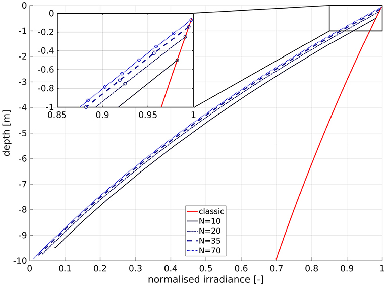
Figure 1. Influence of number of layers N on the attenuation of normalized irradiance for a depth of 10 m. The abscissa is normalized irradiance, and the ordinate is depth. The solid red line is the classic scheme, the other lines are for the IND scheme: solid black is for N = 10, dark blue dashed is for N = 20, bold dashed blue is for N = 35 (as in our model), and dotted blue is for N = 70. The circles in the magnified inset denote the cell center depths of the respective layers.

Another inconsistency arises from the assumption that ln(k/N) is analogous to the attenuation due to SPM $a_{SPM}{\int }_{z_k}^{\zeta }SPM\text{d}z$, as it implies that every layer has a homogeneous concentration of SPM over the entire horizontal domain, i.e., a specific layer carries the same amount of sediment in the Sakgerrak as it does in the German Bight, even though the Skagerrak has more than ten times the depth of the German Bight, and a layer that is close to the surface is unlikely to carry the same content of SPM in both regions. Additionally, as the s-layers are thicker in deeper regions, integrating sediment over depth would imply that deeper regions contain more sediment within the water column. It is thus important to understand that k/N is in fact not a proxy for SPM. However, for layers below the photic zone, where photosynthesis is impossible, the error is biggest, but also least important. The modification can thus serve as a proxy for attenuation due to SPM in the photic zone, yet not as a proxy for actual SPM distribution.

Keeping in mind that the classic scheme assumes constant attenuation over the entire domain when neglecting the influence of phytoplankton, it is helpful to visualize what that implies. While it is impossible to display the sea floor illumination in the IND scheme, due to the noted physical inconsistency, it is possible to compare the 1%- and 10%-depths, as shown in Figure 2. In the classic scheme, if disregarding phytoplankton, the 10%- and 1%-depths are analytically found at $z_{10\%}=\frac{1}{a_w}·ln(0.1)=-64$ m and $z_{1\%}=\frac{1}{a_w}·ln(0.01)=-128$ m, respectively, for a_w = 0.036 1/m. As shown above, the 1%-depth is always lower in the IND scheme than in the classic scheme and the bottom layer irradiance is always lower than 10% of its surface level. Consequently, in areas shallower than 64 m (i.e., the floor would be illuminated in the classic scheme), the IND scheme often has a 1%-depth that is shallower than the 10%-depth of the classic scheme.

FIGURE 2

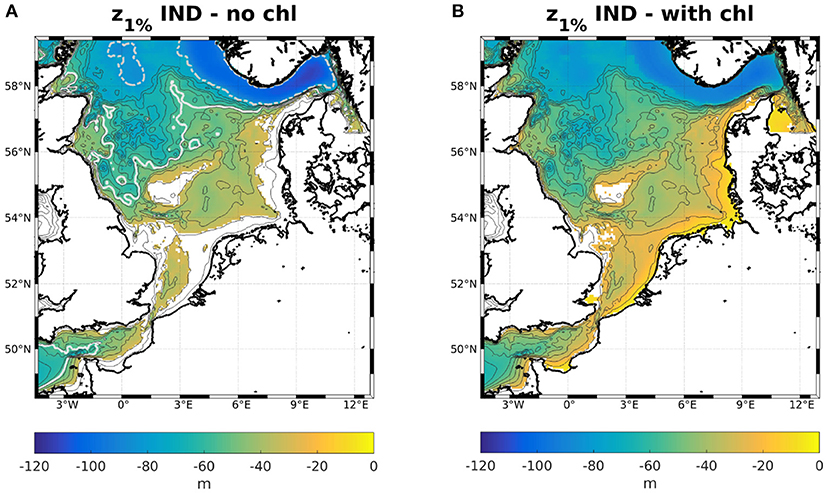
Figure 2. Colors: 1%-depths for the IND scheme (A) neglecting chlorophyll and (B) considering chlorophyll. The dashed gray isoline in (A) is the 1%-, and the white isoline is the 10%-depth of the classic scheme. Blank cells mark areas where the bottom layer irradiance is higher than 1 or 10%, respectively.

Both methods are somewhat unrealistic and must be applied with caution and knowledge of their respective flaws. Trying to make a model of a conglomerate of several notoriously complex and diverse ecosystems in such an oversimplified way as we do will come with its shortcomings. While a more precise approach is certainly desirable for some applications, especially in a more localized domain, we argue for efficiency over precision when trying to show the effects of reducing light availability globally, but more strongly in shallow areas. Furthermore, we stride to make a simple, qualitative study on the effect of heterogeneous reduction of light availability. The IND method has been shown to improve model performance over a large domain with heterogeneous turbidity, while not requiring the costs of a full 3D sediment model (Zhou et al., 2017). The expected results thus justify the use of the IND method.

2.4. Description of Used Data

All of our set-ups of ROMS-CoSiNE are initialized, and in the case of the 3D set-ups also forced at the open boundaries with data taken from AMM7-ERSEM. The Forecasting Ocean Assimilation Model (FOAM, Bell et al., 2003) was applied to the Atlantic Margin Region (40 deg N, 20 deg W to 65 deg N, 13 deg E) with 1/15deg latitudinal and 1/9deg latitudinal resolution (~7 km-square, hence the acronym AMM7), giving reanalyzed hydrodynamic data. The physical core of AMM7 is the Nucleus for European Modeling of the Ocean (NEMO, Madec, 2008), which uses a structured horizontal Arakawa C-grid, as well as a hybrid s-z-grid in the vertical. The physical model is coupled to ERSEM (Baretta et al., 1995; Radach and Lenhart, 1995). In its original formulation, the biological structure ERSEM is immensely complex, compared to that of CoSiNE (Baretta-Bekker et al., 1995; Baretta et al., 1995; Chai et al., 2002; Zhou et al., 2017; Liu et al., 2018), including both a benthic and a pelagic component for a combined total of 31 state variables with decoupled nutrient cycles¹. For reasons of simplicity, benthic modules are often omitted—as in the case of AMM7-ERSEM and ROMS-CoSiNE. CoSiNE is based on a nitrogen cycle, to which carbon, phosphate, and silicate cycles are coupled, and mostly act as nutrient limiting factors. It also does not explicitly model dissolved organic matter (DOM), as ERSEM does. The version of ERSEM that was used in AMM7 is one-dimensional along the vertical axes, and is described in Blackford et al. (2004). We compare our model against AMM7-ERSEM, because (a) our model was built on it, and (b), the available amount of in situ data is rather poor and AMM7-ERSEM has been reanalyzed using the available data.

Because we aim for a simple, inexpensive model, CoSiNE13 is an optimal choice. We accept several strong restrictions for the benefit of efficiency, yet to test the modification of the light treatment, a model like ERSEM or CoSiNE in its 2014 formulation (Xiu and Chai, 2014) would be too complex. Nevertheless, when aiming for accuracy in prediction of chlorophyll and nutrient dynamics, one might consider or even prefer utilizing a more complete and less restrictive ecosystem model.

2.5. Methods of Analysis

To compare magnitudes of phytoplankton bloom as well as horizontal distribution of surface values to measurements and AMM7-ERSEM, monthly means were computed at the surface over the entire domain. We performed area averages over the ICES boxes (see Figure 3, O'Driscoll, 2014). To do so, we first interpolated the ROMS data onto geopotential layers (z-layers). For reasons of comparability, we chose to take the same depth levels as are available for AMM7-ERSEM data via CMEMS (0, 3, 10, 15, 20, 30, 50, 75, 100, 125, 150, 200, 250, 300, 400, and 500 m). To quantify the effect of the modification, the bias and root mean square differences (RMSD) of the area averages, normalized by the total range of chlorophyll for the classic scheme within a box (nbias and nRMSD), were calculated for each z-layer.

FIGURE 3

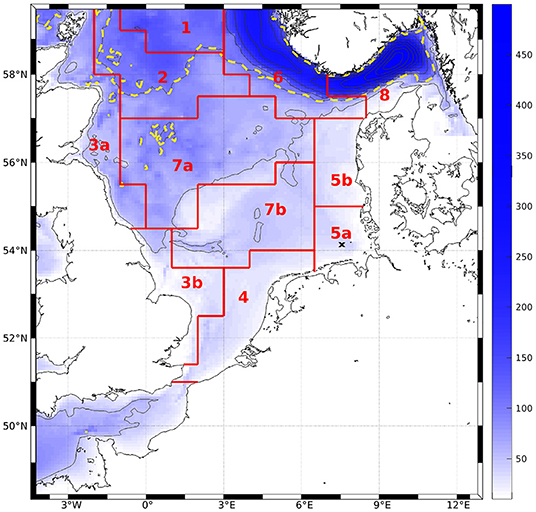
Figure 3. Bathymetry of the model area. Contour intervals are 50 m, dashed line denotes 100 m. Red lines and tags show ICES boxes after O'Driscoll (2014). The black cross marks the station to which Figures 4 and 7 refer.

Utilizing a method applied to Scanfish data (Zhao et al., 2019b), we sorted chlorophyll profiles in the German Bight into four categories: high content in upper layers (HCU) and lower layers (HCL), well mixed profiles (WM) and subsurface chlorophyll maxima (SCM). Zhao et al. (2019b) distinguished between SCM with HCL, with HCU and otherwise well mixed situations, however, due to the relative scarcity of SCM, we do not make this distinction here.

3. Results and Discussion

3.1. Evaluation of the Biological Model

The model simulates a realistic seasonal cycle. Figure 4 shows an example of nitrate, all plankton groups and nitrogenous detritus at depth vs. time in the German Bight (black cross in Figure 1) for the IND scheme. The spring bloom for diatoms occurs earlier than that for small phytoplankton. The microzooplankton feeds on small phytoplankton exclusively, and as the latter is outcompeted by the diatoms, the microzooplankton is also of low concentration. Because the diatoms are more abundant in the second year, the small phytoplankton is almost entirely absent, and subsequently, so is the microzooplankton, not occurring at all in 2013. The year 2012 was slightly colder than 2013, which is why primary production in 2013 was stronger. This also shows in AMM7. The mesozooplankton feeds of diatoms, small phytoplankton, microzooplankton and detritus, for which reason it is present throughout the entire runtime, usually with a phase lag of a few weeks, respective to phytoplankton and detritus. Both diatoms and detritus sink to the floor. This leads the diatoms to accumulate below the surface, where light availability is still high enough.

FIGURE 4

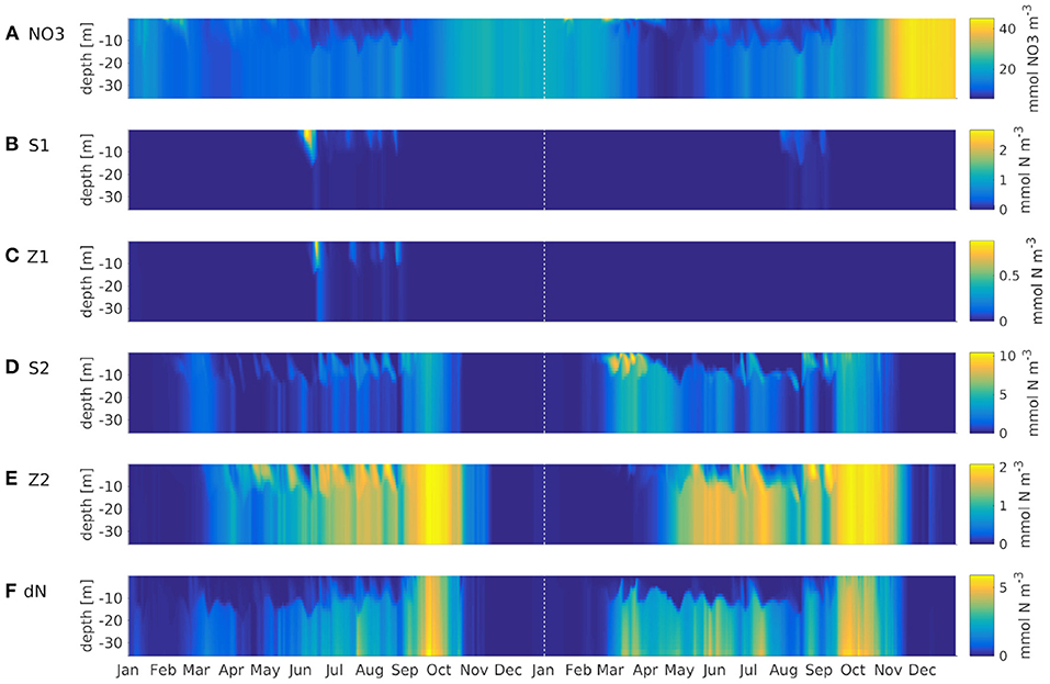
Figure 4. Hovmöller diagrams of ROMS-CoSiNE simulations using the IND scheme at the station marked by the black cross in Figure 1. In top down order, the panels are NO3 (mmol NO3m⁻³) (A), small phytoplankton (B), microzooplankton (C), diatoms (D), mesozooplankton (E) and nitrogenous detritus (F) (all mmol N m⁻³). The dashed vertical line marks the first of January 2013.

A comparison with AMM7-ERSEM data for the same nutrients showed no obvious or critical mismatch. All nutrients recover in the winter of 2012 and 2013 to about the same value they had in the IC. Note that Figure 4 shows output at one particular station in the German Bight, which is a region of strong horizontal turbulence. Thus, no single station is representative of the entire region. Area averages reveal that all nutrients do indeed recover (not shown). Given the immense complexity of ERSEM and AMM7, relative to our model, and the fact that we are comparing to reanalyzed data, could explain some of the quantitative differences. The comparisons to AMM7 and CCI data (Figure 5) show that ROMS-CoSiNE matches the spacial distribution patterns of the chlorophyll dynamics in the North Sea, and in some cases even better than AMM7-ERSEM does. ROMS-CoSiNE shows an overestimation of chlorophyll along the south western shore, and an underestimation in the deeper, northern North Sea, as well as the East Anglia Plume. However, the horizontal distribution patterns of ROMS-CoSiNE (both schemes) and CCI are very alike.

FIGURE 5

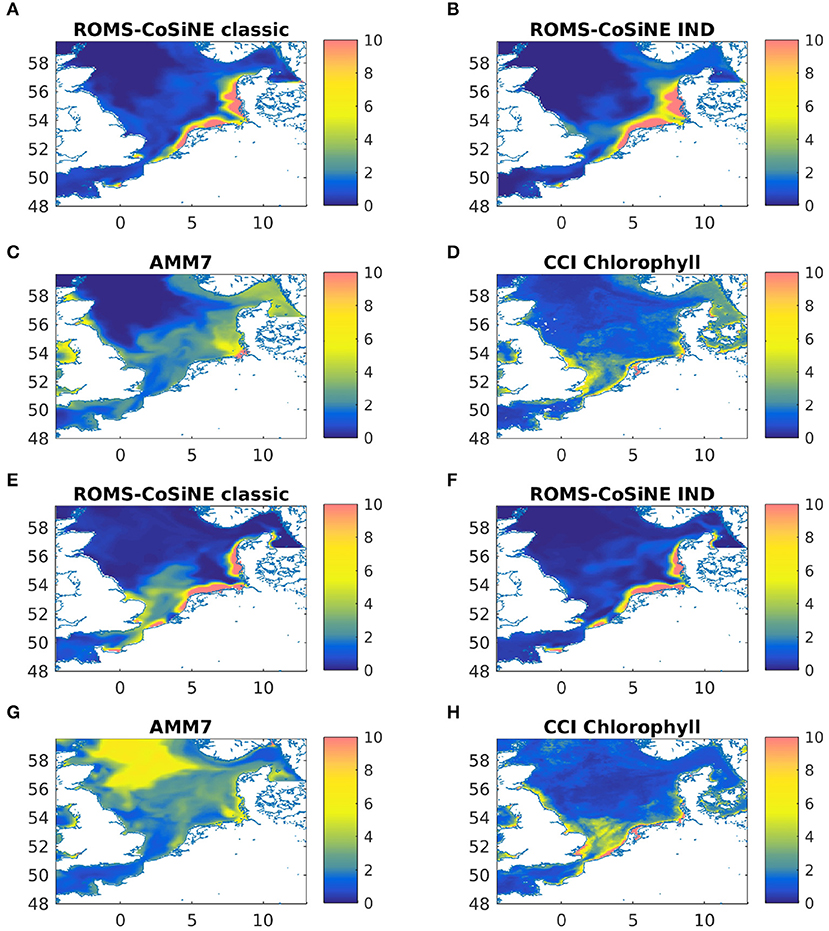
Figure 5. Monthly means of chlorophyll-a [mgChl − am⁻³] for ROMS-CoSine in the classic formulation (A,E), and the IND formulation (B,F), as well as AMM7 (C,G), and CCI data (D,H) for March 2013 (A–D) and May 2013 (E–H).

The area averages of both schemes and AMM7 at 3 m depth, as well as ICES bottle data and FerryBox data of chlorophyll-a is shown in Figure 6. In the north western boxes, the data availability is rather scarce, however there, the CCI data (Figure 5) can be taken as a good point of reference. The agreement between models and measurements are of varying degree, both locally and temporarily. Many of the differences between the models and data are found for both models. Furthermore, the in situ data consists of subsampled data from a large domain that shows significant horizontal variability. We have filtered the bottle and FerryBox data points so that only regions of salinity greater than 30PSU were considered. This was done to exclude data points taken in river mouths or very close to the shore (e.g., the Wadden Sea), where processes which we cannot resolve might influence the phytoplankton growth. Furthermore, we have taken daily averages, in case there were multiple data points per day. The comparison shows that our simulations are realistic, qualitatively speaking. Pätsch and Kühn (2008) have performed a study using a 3D ecosystem model (ECOHAM) in the North Sea for the years 1993 to 1996. Simulated nitrate and chlorophyll values in the upper layers (their Figure 6) were found to largely agree with our simulations, patternwise. Magnitudes were lower in ROMS-CoSiNE for box 1 and 7 (compare Figure 6 to Pätsch and Kühn, 2008, their Figures 6D,E—note that AMM7 is overestimating here), and higher for box 5a (Pätsch and Kühn, 2008, their Figure 6F). Another reason for differences could be that we are comparing different time periods with 17 years between their study and ours. Note also that while we are comparing area averages, the areas we average over are of different size than those (Pätsch and Kühn, 2008) average over.

FIGURE 6

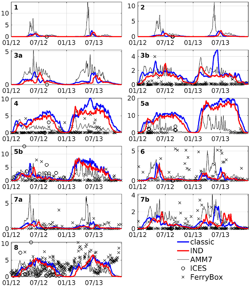
Figure 6. Area averages of chlorophyll at 3 m depth in units of mg Chl m⁻³. Blue line is the classic scheme, red is the IND scheme, black is AMM7, black crosses is FerryBox data and black circles is ICES bottle data.

3.2. Comparison of the Two Light Schemes

The coupling of CoSiNE in the classic formulation to ROMS increases the total amount of parallel computation time by 226% with respect to a physical run. The inclusion of the IND scheme does not influence the runtime, relative to the classic formulation by any significant number (0.57%).

The effect of the IND scheme is visualized in Figure 7, which shows normalized irradiance attenuated with depth, taking phytoplankton absorption into account. Without phytoplankton present (i.e., winter months), the normalized irradiance in the classic scheme is well above 10% at the bottom, while the 10%-depth in the IND scheme is at around 21 m by default. While the chlorophyll attenuation coefficient is the same in both set-ups, the factor k/N has a strong effect in lower layers, causing the 10%-depth to be reduced by half in times of high chlorophyll-a abundance. In the classic scheme, the remaining light never reaches a value of 1% or lower, while it does in the IND scheme.

FIGURE 7

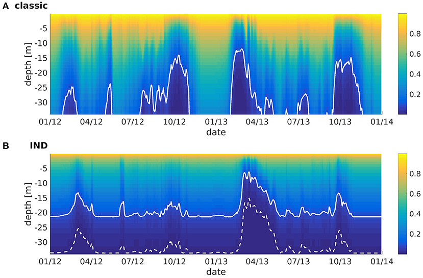
Figure 7. Normalized irradiance at depth vs. time for ROMS-CoSiNE at the station marked by the black cross in Figure 1 using (A) the classic formulation and (B) the IND scheme. The solid line denotes the 10%-, and the dashed line the 1%-depth.

Floeter et al. (2017) have performed measurements in the German Bight in similar positions as station used in Figures 1, 4, 7. Using a hyperspectral TriOS Ramses-ACC irradiance sensor, they calculated the 1%-depths along transects through wind farms. The measured depths ranged between 26 and 21 m in July 2014 (see Floeter et al., 2017, their Figure 11). As can be seen in Figure 7, the IND scheme is thus more realistic here, showing similar (if slightly too great) 1%-depths in the summer months of 2012 and 2013. Note that we neglect the effects of CDOM, which are potentially significant at this particular station in the German Bight (compare to e.g., Painter et al., 2018).

The nRMSD and nbias are shown in Figure 8. While the patterns of both quantities are largely similar, there is often times a pronounced nRMSD at the surface, while there is no or only a small nbias there. This is explained by a difference in timing with no or little difference in magnitude (as can be seen in Figure 6). Note that the maxima of nRMSD and nbias are not found in the bottom layers but around the boxes' average depths. Over large areas along the southern shore, the North Sea is shallower than 10 m, yet, our model has no dryfalling and a minimum depth is prescribed as 10 m. Around a third of box 5a is shallower than 15 m (compare Figure 1), which explains why the largest nRMSD and nbias are found there at 10 m depth (Figure 8), as we are comparing the area averages that have been interpolated onto a z-grid. The two boxes where the largest nRMSD and nbias do not occur at the boxes' respective average depths (boxes 6 and 8) are so deep that in both schemes, the lowest layers are outside of the photic zone. Accordingly, there is neither significant nbias nor nRMSD in the bottom layers of these boxes. The least pronounced effects on both nRMSD and nbias are found in boxes 1 and 6, where there is mostly a shift in timing (see also Figure 6). The largest values for nRMSD and nbias are found in the lower layers of box 7a (central North Sea), a box that is remote from any river influx and has an average depth of 62 ± 5 m (which is close to the 10%-depth of 64 m in the classic scheme). This largely falls into a domain which Capuzzo et al. (2015) described as seasonally stratified and for which they found average Secchi depths between z_SD = 4.11 ± 1.3 m in winter and z_SD = 10.61 ± 3.56 m in summer. According to Lee et al. (2015), the Secchi depth is approximately the inverse of the downwelling attenuation coefficient k_d, and given that $k_d=-z_{1\%}^{-1}ln(\frac{I(z_{1\%})}{I_0})$, it follows that z_SD ≈ 0.22z_1%. Figure 3B shows that the IND scheme is close to this, with z_1%-values ranging between roughly 20 and 70 m, and thus Secchi depths of roughly 4 to 15 m on average. The classic scheme never reaches values below z_SD ≈ 30 m (not shown).

FIGURE 8

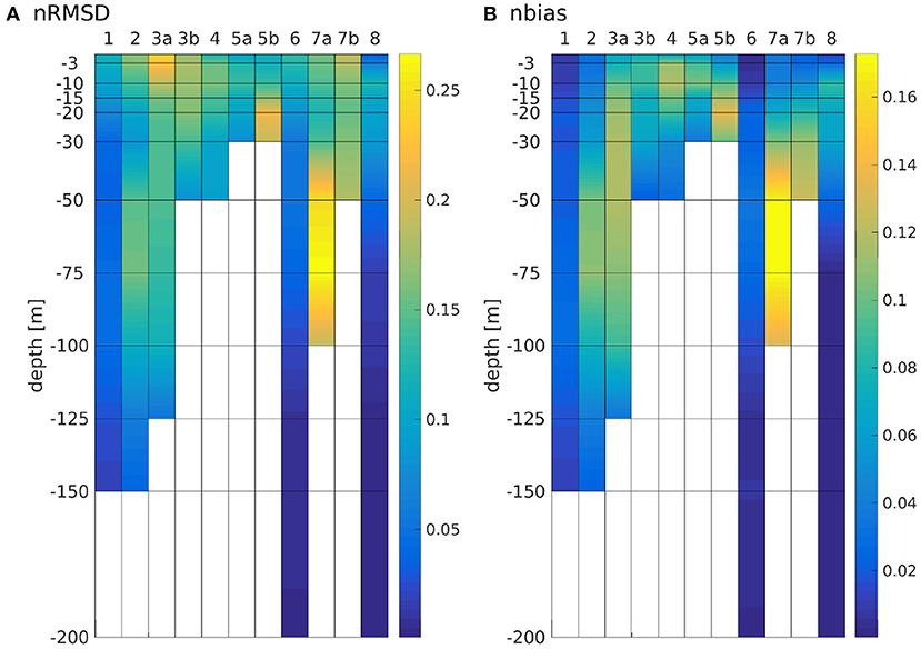
Figure 8. Normalized RMSD (A) and bias (B) of chlorophyll between classic and IND for all boxes.

For the IND scheme, as Figures 9C,D show, the largest reductions of both the 1%- and 10%-depths with respect to the total water depth are found in the southern North Sea, along the Dutch, German, and Danish coasts. This is likely due to the overestimation of diatoms there. The same can be seen in the classic scheme (not shown). However, all areas where the relative change in 1%- and 10%-depths are greater than 15% are characterized by large riverine nutrient influxes. In other shallow regions, e.g., at the Oyster grounds (box 7b), the reductions are not as pronounced. The areas of the greatest absolute change are thus areas that are light limited and those with the greatest relative change are nutrient limited (compare e.g., Zhao et al., 2019a, their Figure 3). In absolute terms, the greatest reduction of the 1%- and 10%-depths are found along the Norwegian coast and in the Skagerrak, which is largely due to the greater water depth (Figures 9A,B). Figure B.1 shows the ratios between 1%- and 10%-depths both with and without considering chlorophyll specific attenuation. The ratio noticeably increases in the areas where the absolute reductions of the 1%- and 10%-depths are greatest (Figures 9A,B), which is due to the self shadowing of phytoplankton. Capuzzo et al. (2015) show a map of sea floor illumination in the area of the East Anglia Plume (their Figure 3), classifying regions that have been illuminated before and after 1950 (dark blue), only were illuminated before 1950 (lighter blue), or were never illuminated (light blue). Noticeably, the areas that are still illuminated today match the areas in our model were the average bottom irradiance is greater than 1% of the surface irradiance (Figure B.1B).

FIGURE 9

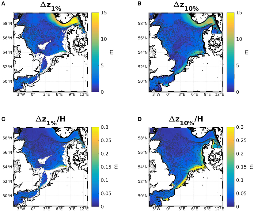
Figure 9. Differences of the 2 year means of the 1%- (A,C) and 10%-depths (B,D) with chlorophyll specific attenuation minus without. Absolute values are shown in (A,B), and (C,D) show the same, normalized by the local water depth.

The area averaged chlorophyll differences show that there is merely a reduction of magnitude, but no vertical shift of a subsurface maximum between the two schemes. From Figure 6, we can see that in box 7b, there is one strong peak of chlorophyll in the summer of 2013 for the classic scheme, but in the IND scheme, there is one peak in spring and one in autumn, both being smaller than the peak in the classic scheme. The biannual mean of the differences are low at the surface, because approximately the same amount of chlorophyll is produced in both schemes, yet the nRMSD responds to the different temporal behavior of the blooms (Figure 8). In the Skagerrak, there are biases of 2mg Chl m⁻³, reaching depths of up to 50 m and prevailing for several months (not shown). This is due to the inclusion of parts of the Kattegat in Box 8, which is rather shallow, and heavily influenced by the Baltic outflow. All other deep boxes do show differences, but they are mostly differences in timing and less in magnitude. As Figure 6 shows, the blooms in these boxes are comparably short.

Comparing our results for the German Bight (box 5a, Figure 10) to Zhao et al. (2019b their Figure 4), there are a few differences, but the overall agreement is reasonably good, and more so with the implementation of a modified light regime. There are fewer stratified profiles in the IND case, compared to the classic case, in almost all areas and at almost all times, except areas that are of depths between 15 and 25 m, where the IND scheme shows generally more stratified profiles. In regions deeper than 15 m, there are more HCU situations in the IND scheme than in the classic scheme. There are relatively fewer SCM situations in ROMS-CoSiNE than there are in the scanfish data, analyzed by Zhao et al. (2019b). A likely reason for this is the relatively coarse resolution of 35 layers. Due to the overestimation of winter chlorophyll, there are more stratified profiles in early months in the model than there are in the Scanfish data. SCM tend to occur in shallower regions in the IND scheme, compared to the classic scheme and the Scanfish data. HCL situations are more frequent than HCU, because the diatoms, which are prevalent in the German Bight, sink to the floor.

FIGURE 10

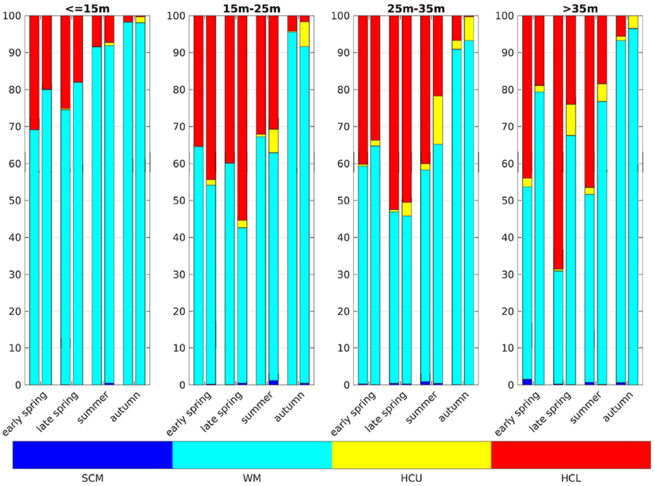
Figure 10. Categories of vertical chlorophyll profiles in the German Bight. Dark blue are subsurface chlorophyll maxima (SCM), turquois are well mixed profiles (WM), yellow are high chlorophyll content in upper layers (HCU), and red are high chlorophyll content in lower layers (HCL). The left bars show the classic scheme and the right the IND. Early spring is March and April, late spring is May, summer is June, July, and August, and autumn is September, following the classification of Zhao et al. (2019b).

Figure 11 shows depth integrated chlorophyll for both schemes. Especially in boxes that are shallow and/or have large riverine nutrient influence (3b to 6, 7b, and 8), the spring bloom peaks are of similar, and sometimes higher magnitude than the classic scheme. There is a time shift of up to several months in both years (explaining the presence of nRMSD, yet absence of bias in the upper layers; see above and Figure 8). The growth throughout the rest of the year shows no shift in timing, but often significantly lower magnitudes. In the remaining boxes (1 to 4a, and 7a), the growth is generally weaker and slower.

FIGURE 11

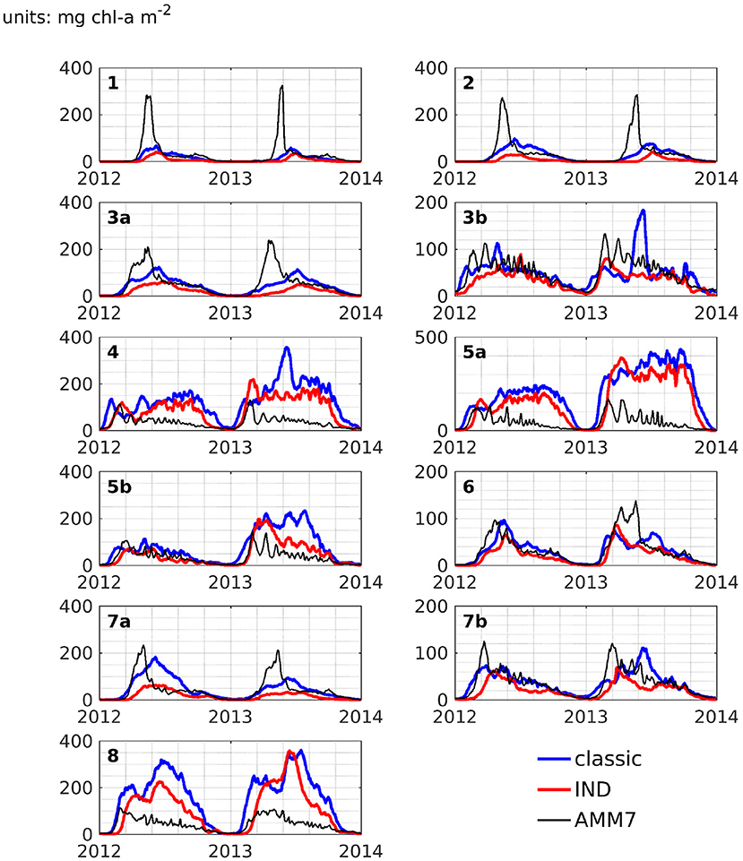
Figure 11. Depth integrated area averages of chlorophyll-a for ROMS-CoSiNE in the classic formulation (blue) and the IND scheme (red), as well as AMM7 (black), for all areas.

The comparisons of area averages (Figures 6, 11), as well as that of monthly means of surface chlorophyll to CCI and AMM7 data (Figure 5) show that for some situations, the classic scheme is closer to the data (more in the deep northern and western areas), and for others the IND does. It can be noted that the agreement between AMM7 and ROMS-CoSiNE is generally good, with some glaring differences (AMM7 chl is higher in the deeper, northern regions, but lower near the Belgian, Dutch, and German coast). The inclusion of the IND scheme helps to bring ROMS-CoSiNE and AMM7 closer together in some areas (e.g., boxes 4, 5a, 5b), but in others, it does the opposite (e.g., boxes 1, 2, 3a, 7a). Incidentally, the deep, northern boxes 1 to 3a are the ones where AMM7 agrees least with CCI data (Figure 5).

4. Conclusions

A functioning ecosystem model was established, which is capable of reproducing a realistic seasonal cycle of nutrients, phyto- and zooplankton, as well as detritus. The horizontal distribution of chlorophyll matches that of measurements. Because the model is relatively cheap to run, it gives a good starting point for further investigations of light climate, although adjustments will need to be made to accommodate the effects of temporal variability and CDOM. To the best of our knowledge, there has not been a published application of ROMS-CoSiNE in the North Sea. We have shown that ROMS is capable of giving reliable numeric simulations of the physical North Sea. CoSiNE is capable of simulating important aspects of its biology. For the purpose of a sensitivity study, the model produces results of sufficient accuracy.

The reduction of light availability leads to weaker total production of chlorophyll-a. Because the modification reduces light availability in the entire domain, this was an expected result. For all boxes, the reduced light availability in the IND scheme expresses itself in three ways: the spring bloom peaks occur later, their magnitudes are weaker, and the magnitude of growth after the spring bloom is weakened. However, these three characteristics need not be present in the same extremity for all boxes. Generally, deep boxes with little terrestrial nutrient input (1, 2, and 3a) show the least change in total magnitude. The far greatest total reductions in growth are found in regions with large river inputs. Because there is no nutrient limitation there, light limitation is dominant. The total magnitudes are also larger there, allowing for greater total reduction. In relative terms, the greatest impact is found in deep areas with low magnitudes and strong nutrient limitation. As regions of high terrestrial water input are typically rich in CDOM (e.g., Painter et al., 2018), the inclusion of CDOM specific attenuation is expected to further increase the total reduction of magnitude in those areas.

The IND scheme thus provides the expected results exactly where they are desired, but also brings undesired results elsewhere. A hybrid scheme could help correct for this, where the IND scheme (or a similar modification) is active in a nearshore environment and inactive in domains that can be seen as case 1 waters, are deep enough for SPM to not play a role, or where there is otherwise naturally little SPM effect on light attenuation. For turbid regions, such as estuaries or specific marginal seas or coastal subbasins (e.g., German Bight, East China Sea, San Francisco Bay, Chesapeake Bay—all areas where CoSiNE has been used), the global use of the IND scheme may be more desirable than coupling to a sediment and wind wave module, for reasons of simplicity, affordability, and qualitatively similar results. The use of a simple weighting function (e.g., activating the IND scheme for all depths below a threshold value, or activation via a prescribed mask) can make the scheme more flexible without defeating the purpose of having a very affordable scheme that is also easy to implement. Furthermore, ROMS has the capability (as do many other models), to distribute the upper layers (almost) equally, along geopotential surfaces, especially in deeper areas. This is generally desirable for physical applications in areas of large bottom slopes and strong stratification, but it is not ideal for the use of the IND scheme. Again, this may be controlled for by weighting functions.

The SPM attenuation proxy we apply has several important short-comings: (a) we only account for inorganic SPM, while organic SPM is left out [more advanced biological models can account for organic SPM (e.g., Xiu and Chai, 2014)]; (b) the proxy is dependent on bathymetry only, while SPM content in a water column itself has several important influencing factors, such as bottom stress due to wind waves and currents (which is time dependent), grain size and the soil texture of the sea floor (which is horizontally varying, and which can be advected); (c) the vertical distribution of SPM content is approximated by a dependency on bathymetry following s-layers, i.e., a model specific quantity, and not a physical one; (d) the actual SPM content need not be (pseudo) linearly or even monotonously increasing with depth, as we assume it to be; (e) our SPM proxy is, mathematically speaking, unstable, because it contains a singularity (which is numerically speaking outside of our domain). Nevertheless, it is extremely simple to implement and has proven to be effective (Zhou et al., 2017), while being literally no more expensive than the classic approach, without the need to employ an online-coupled sediment and wind wave module, next to the existing configuration. Given that the omission of the modification is equally unphysical, but considerably less realistic, we deem its use justified.

As stated in the introduction, we do not consider CDOM in this work. However, CDOM has been shown in numerous works to be one of the key influences of water clarity (e.g., Dupont and Aksnes, 2013; Urtizberea et al., 2013; Opdal et al., 2019). In the context of coastal ocean darkening over the twentieth century, as it is suggested by multiple studies (e.g., Dupont and Aksnes, 2013; Capuzzo et al., 2015; Opdal et al., 2019), one cannot ignore the role CDOM plays. Future works on the subject of the coastal underwater light field will have to include the effects of CDOM, be it through directly modeling it, as (e.g., Xiu and Chai, 2014) do, or inversely modeling it by applying linear relationships with salinity (e.g., Bowers et al., 2004; Bowers and Brett, 2008; Painter et al., 2018). It is our intention to include CDOM in future works. Furthermore, SPM contents in the North Sea are subject to both seasonal (e.g., van der Molen et al., 2009; Dobrynin et al., 2010; Gohin, 2011) and interannual variability (e.g., van der Molen et al., 2009; Capuzzo et al., 2015; Wilson and Heath, 2019). The IND scheme cannot model temporal effects and is thus unsuitable for use in long term studies. For such purposes, one might use offline data, or directly model SPM.

Data Availability Statement

The datasets generated for this study are available on request to the corresponding author.

Author Contributions

The practical work and majority of the writing was carried out by DT in the context of his Ph.D. study, under the supervision of ES, within the Coastal Ocean Darkening project, which is headed by OZ. ES and OZ directed DT, and reviewed and edited the text and figures.

Funding

This work was carried out within the project Coastal Ocean Darkening (grant no. ZN3175), funded by the Ministry of Science and Culture of the German federal state of Lower Saxony.

Conflict of Interest

The authors declare that the research was conducted in the absence of any commercial or financial relationships that could be construed as a potential conflict of interest.

Acknowledgments

The study has been conducted using E.U. Copernicus Marine Service Information. The code used to compute FES2014, was developed in collaboration between Legos, Noveltis, CLS Space Oceanography Division and CNES, and is available under GNU General Public License. Atmospheric forcing data was provided by the NOAA ESRL Physical Sciences Division, Boulder, Colorado, USA, and taken from their website at http://www.esrl.noaa.gov/psd/.

For their helpful insight, and guidance, we would like to thank Fei Chai, Feng Zhou, Johannes Pein, and Sebastian Grayek.

Supplementary Material

The Supplementary Material for this article can be found online at: https://www.frontiersin.org/articles/10.3389/fmars.2019.00816/full#supplementary-material

Footnote

1. ^Note, that we are comparing ERSEM to a version of CoSiNE with 13 state variables (CoSiNE13). There exists a version of CoSiNE with 31 pelagic state variables (CoSiNE31), utilizing a spectral treatment of light, which is applied to the Pacific ocean, hence not requiring a benthic module (Xiu and Chai, 2014).

References

Baretta, J., Ebenhöh, W., and Ruardij, P. (1995). The European regional seas ecosystem model, a complex marine ecosystem model. Netherlands J. Sea Res. 33, 233–246. doi: 10.1016/0077-7579(95)90047-0

CrossRef Full Text | Google Scholar

Baretta-Bekker, J., Baretta, J., and Koch Rasmussen, E. (1995). The microbial food web in the european regional seas ecosystem model. Netherlands J. Sea Res. 33, 363–379. doi: 10.1016/0077-7579(95)90053-5

CrossRef Full Text | Google Scholar

Baschek, B., Schroeder, F., Brix, H., Riethmüller, R., Badewien, T., Breitbach, G., et al. (2017). The coastal observing system for Northern and Arctic seas (COSYNA). Ocean Sci. 13, 379–410. doi: 10.5194/os-13-379-2017

CrossRef Full Text | Google Scholar

Bell, M., Barciela, R., Hines, A., Martin, M., McCulloch, M., and Storkey, D. (2003). The forecasting ocean assimilation model (FOAM) system. Elsevier Oceanogr. Ser. 69, 197–202. doi: 10.1016/S0422-9894(03)80033-8

CrossRef Full Text | Google Scholar

Bissett, W., Schofield, O., Scott, G., Cullen, J., Miller, W., Plueddemann, A., et al. (2001). Resolving the impacts and feedback of ocean optics on upper ocean ecology. Oceanography 14, 30–53. doi: 10.5670/oceanog.2001.22

CrossRef Full Text | Google Scholar

Bissett, W., Walsh, J., Dieterle, D., and Carder, K. (1999). Carbon cycling in the upper waters of the Sargasso Sea: I. Numerical simulation of differential carbon and nitrogen fluxes. Deep Sea Res. Part I Oceanogr. Res. Pap. 42, 205–269. doi: 10.1016/S0967-0637(98)00062-4

CrossRef Full Text | Google Scholar

Blackford, J., Allen, J., and Gilbert, F. (2004). Ecosystem dynamics at six contrasting sites: a generic modelling study. J. Mar. Syst. 52, 191–215. doi: 10.1016/j.jmarsys.2004.02.004

CrossRef Full Text | Google Scholar

Bowers, D., and Brett, H. (2008). The relationship between CDOM and salinity in estuaries: an analytical and graphical solution. J. Mar. Syst. 73, 1–7. doi: 10.1016/j.jmarsys.2007.07.001

CrossRef Full Text | Google Scholar

Bowers, D., Evans, D., Thomas, D., Ellis, K., and Williams, P. B. (2004). Interpreting the colour of an estuary. Estuar. Coast. Shelf Sci. 59, 13–20. doi: 10.1016/j.ecss.2003.06.001

CrossRef Full Text | Google Scholar

Cahill, B., Schofield, O., Chant, R., Wilkin, J., Hunter, E., Glenn, S., et al. (2008). Dynamics of turbid buoyant plumes and the feedbacks on near-shore biogeochemistry and physics. Geophys. Res. Lett. 35. doi: 10.1029/2008GL033595

CrossRef Full Text | Google Scholar

Capuzzo, E., Stephens, D., Silva, T., Barry, J., and Forster, R. (2015). Decrease in water clarity of the southern and central North Sea during the 20th century. Glob. Change Biol. 21, 2206–2214. doi: 10.1111/gcb.12854

PubMed Abstract | CrossRef Full Text | Google Scholar

Chai, F., Dugdale, R., Peng, T.-H., Wilkerson, F., and Barber, R. (2002). One-dimensional ecosystem model of the equatorial Pacific upwelling system. Part I: model development and silicon and nitrogen cycle. Deep Sea Res. II Top. Stud. Oceanogr. 49, 2713–2745. doi: 10.1016/S0967-0645(02)00055-3

CrossRef Full Text | Google Scholar

Daewel, U., and Schrum, C. (2013). Simulating long-term dynamics of the coupled North Sea and Baltic Sea ecosystem with ECOSMO II: model description and validation. J. Mar. Syst. 119–120, 30–49. doi: 10.1016/j.jmarsys.2013.03.008

CrossRef Full Text | Google Scholar

Dobrynin, M., Gayer, G., Pleskachevsky, A., and Günther, H. (2010). Effect of waves and currents on the dynamics and seasonal variations of suspended particulate matter in the North Sea. J. Mar. Syst. 82, 1–20. doi: 10.1016/j.jmarsys.2010.02.012

CrossRef Full Text | Google Scholar

Dupont, N., and Aksnes, D. (2013). Centennial changes in water clarity of the Baltic Sea and the North Sea. Estuar. Coast. Shelf Sci. 131, 282–289. doi: 10.1016/j.ecss.2013.08.010

CrossRef Full Text | Google Scholar

Evans, G., and Parslow, J. (1985). A model of annual plankton cycles. Biol. Oceanogr. 3, 328–347.

Google Scholar

Fasham, M., Ducklow, H., and McKelvie, S. (1990). A nitrogen-based model of plankton dynamics in the oceanic mixed layer. J. Mar. Res. 48, 591–639. doi: 10.1357/002224090784984678

CrossRef Full Text | Google Scholar

Floeter, J., Van Beusekom, J., Auch, D., Callies, U., Carpenter, J., Dudeck, T., et al. (2017). Pelagic effects of offshore wind farm foundations in the stratified North Sea. Prog. Oceanogr. 156, 154–173. doi: 10.1016/j.pocean.2017.07.003

CrossRef Full Text | Google Scholar

Gohin, F. (2011). Annual cycles of chlorophyll-a, non-algal suspended particulate matter, and turbidity observed from space and in-situ in coastal waters. Ocean Sci. 7, 705–732. doi: 10.5194/os-7-705-2011

CrossRef Full Text | Google Scholar

Haidvogel, D., Arango, H., Hedstrom, K., Beckmann, A., Malanotte-Rizzoli, P., and Shchepetkin, A. (2000). Model evaluation experiments in the North Atlantic Basin: simulations in nonlinear terrain-following coordinates. Dyn. Atmos. Ocean 32, 239–281. doi: 10.1016/S0377-0265(00)00049-X

CrossRef Full Text | Google Scholar

Harvey, E., Walve, J., Andersson, A., Karlson, B., and Kratzer, S. (2019). The effect of optical properties on secchi depth and implications for eutrophication management. Front. Mar. Sci. 5:496. doi: 10.3389/fmars.2018.00496

CrossRef Full Text | Google Scholar

Kühn, W., and Radach, G. (1997). A one-dimensional physical-biological model study of the pelagic nitrogen cycling during the spring bloom in the northern North Sea (FLEX '76). J. Mar. Res. 55, 687–734. doi: 10.101357/0022240973224229

CrossRef Full Text | Google Scholar

Lee, Z., Shang, S., Hu, C., Du, K., Weidemann, A., Hou, W., et al. (2015). Secchi disk depth: a new theory and mechanistic model for underwater visibility. Remote Sens. Environ. 169, 139–149. doi: 10.1016/j.rse.2015.08.002

CrossRef Full Text | Google Scholar

Lenhart, H., Radach, G., Backhaus, J., and Pohlmann, T. (1995). Simulations of the north sea circulation, its variability, and its implementation as hydrodynamical forcing in ERSEM. Netherlands J. Sea Res. 33, 271–299. doi: 10.1016/0077-7579(95)90050-0

CrossRef Full Text | Google Scholar

Liu, Q., Chai, F., Dugdale, R., Chao, Y., Xue, H., Rao, S., et al. (2018). San Francisco Bay nutrients and plankton dynamics as simulated by a coupled hydrodynamic-ecosystem model. Continent. Shelf Res. 161, 29–48. doi: 10.1016/j.csr.2018.03.008

CrossRef Full Text | Google Scholar

Madec, G. (2008). NEMO Ocean Engine. Technical report, Institut Pierre-Simon Laplace (IPSL).

Google Scholar

Mobley, C., Chai, F., Xiu, P., and Sundman, L. (2015). Impact of improved light calculations on predicted phytoplankton growth and heating in an idealized upwelling-downwelling channel geometry. J. Geophys. Res. 120, 875–892. doi: 10.1002/2014JC010588

CrossRef Full Text | Google Scholar

Moll, A. (1997). Phosphate and plankton dynamics during a drift experiment in the German Bight: simulation of phosphorus-related plankton production . Mar. Ecol. Prog. Ser. 156, 289–297. doi: 10.3354/meps156289

CrossRef Full Text | Google Scholar

Moll, A. (1998). Regional distribution of primary production in the North Sea simulated by a three-dimensional model. J. Mar. Syst. 162, 151–170. doi: 10.1016/S0924-7963(97)00104-8

CrossRef Full Text | Google Scholar

O'Driscoll, K. (2014). Air-sea exchange of legacy POPs in the North Sea based on results of fate and transport, and shelf-sea hydrodynamic ocean models. Atmosphere 5, 156–177. doi: 10.3390/atmos5020156

CrossRef Full Text | Google Scholar

Opdal, A., Lindemann, C., and Aksnes, D. (2019). Centennial decline in North Sea water clarity causes strong delay in phytoplankton bloom timing. Glob. Change Biol. 25, 3946–3953. doi: 10.1111/gcb.14810

PubMed Abstract | CrossRef Full Text | Google Scholar

Painter, S., Lapworth, D., Woodward, E., Kroeger, S., Evans, C., Mayor, D., et al. (2018). Terrestrial dissolved organic matter distribution in the North Sea. Sci. Total Environ. 630, 630–647. doi: 10.1016/j.scitotenv.2018.02.237

PubMed Abstract | CrossRef Full Text | Google Scholar

Pätsch, J., and Kühn, W. (2008). Nitrogen and carbon cycling in the North Sea and exchange with the North Atlantic—A model study. Part I. Nitrogen budget and fluxes. Continent. Shelf Res. 28, 767–787. doi: 10.1016/j.csr.2007.12.013

CrossRef Full Text | Google Scholar

Radach, G., and Lenhart, H. (1995). Nutrient dynamics in the north sea: fluxes and budgets in the water column derived from ESEM . Netherlands J. Sea Res. 33, 301–335. doi: 10.1016/0077-7579(95)90051-9

CrossRef Full Text | Google Scholar

Schrum, C., Alekseeva, I., and St. John, M. (2006a). Development of a coupled physical–biological ecosystem model ECOSMO: Part I: model description and validation for the North Sea. J. Mar. Syst. 61, 79–99. doi: 10.1016/j.jmarsys.2006.01.005

CrossRef Full Text | Google Scholar

Schrum, C., St. John, M., and Alekseeva, I. (2006b). ECOSMO, a coupled ecosystem model of the North Sea and Baltic Sea: Part II. Spatial-seasonal characteristics in the North Sea as revealed by EOF analysis. J. Mar. Syst. 61, 100–113. doi: 10.1016/j.jmarsys.2006.01.004

CrossRef Full Text | Google Scholar

Song, Y., and Haidvogel, D. (1994). A semi-implicit ocean circulation model using a generalized topography-following coordinate system. J. Comput. Phys. 115, 228–244. doi: 10.1006/jcph.1994.1189

CrossRef Full Text | Google Scholar

Umlauf, L., and Burchard, H. (2003). A generic length-scale equation for geophysical turbulence models. J. Mar. Res. 61, 235–265. doi: 10.1357/002224003322005087

CrossRef Full Text | Google Scholar

Urtizberea, A., Dupont, N., Rosland, R., and Aksnes, D. (2013). Sensitivity of euphotic zone properties to CDOM variations in marine ecosystem models. Ecol. Model. 256, 16–22. doi: 10.1016/j.ecolmodel.2013.02.010

CrossRef Full Text | Google Scholar

van der Molen, J., Bolding, K., Greenwood, N., and Mills, D. K. (2009). A 1-D vertical multiple grain size model of suspended particulate matter in combined currents and waves in shelf seas. J. Geophys. Res. 114, 148–227. doi: 10.1029/2008JF001150

CrossRef Full Text | Google Scholar

Warner, J., Sherwood, C., Arango, H., and Signell, R. (2005). Performance of four turbulence closure methods implemented using a generic length scale method. Ocean Model. 8, 81–113. doi: 10.1016/j.ocemod.2003.12.003

CrossRef Full Text | Google Scholar

Wilson, R., and Heath, M. (2019). Increasing turbidity in the North Sea during the 20th century due to changing wave climate. Ocean Sci. 15, 1615–1625. doi: 10.5194/os-15-1615-2019

CrossRef Full Text | Google Scholar

Xiu, P., and Chai, F. (2014). Connections between physical, optical and biogeochemical processes in the Pacific Ocean. Prog. Oceanogr. 122, 30–53. doi: 10.1016/j.pocean.2013.11.008

CrossRef Full Text | Google Scholar

Zhao, C., Daewel, U., and Schrum, C. (2019a). Tidal impacts on primary production in the North Sea. Earth Syst. Dyn. 10, 287–317. doi: 10.5194/esd-10-287-2019

CrossRef Full Text | Google Scholar

Zhao, C., Maerz, J., Hofmeister, R., Roettgers, R., Wirtz, K., Riethmüller, R., et al. (2019b). Characterizing the vertical distribution of chlorophyll a in the German Bight. Continent. Shelf Res. 175, 127–146. doi: 10.1016/j.csr.2019.01.012

CrossRef Full Text | Google Scholar

Zhou, F., Chai, F., Huang, D., Xue, H., Chen, J., Xiu, P., et al. (2017). Investigation of hypoxia off the Changjiang Estuary using a coupled model of ROMS-CoSiNE. Prog. Oceanogr. 159, 237–254. doi: 10.1016/j.pocean.2017.10.008

CrossRef Full Text | Google Scholar

Zielinski, O., Llinas, O., Oschlies, A., and Reuter, R. (2002). Underwater light field and its effect on a one-dimensional ecosystem model at station ESTOC, north of the Canary Islands. Deep Sea Res. II 49, 3529–3542. doi: 10.1016/S0967-0645(02)00096-6

CrossRef Full Text | Google Scholar